Abstract
The article deals with sensor fusion and real-time calibration in a homogeneous inertial sensor array. The proposed method allows for both estimating the sensors’ calibration constants (i.e., gain and bias) in real-time and automatically suppressing degraded sensors while keeping the overall precision of the estimation. The weight of the sensor is adaptively adjusted according to the RMSE concerning the weighted average of all sensors. The estimated angular velocity was compared with a reference (ground truth) value obtained using a tactical-grade fiber-optic gyroscope. We have experimented with low-cost MEMS gyroscopes, but the proposed method can be applied to basically any sensor array.
Keywords: calibration, data averaging, MEMS gyroscope, sensor fusion
1. Introduction
MEMS inertial sensors (i.e., gyroscopes and accelerometers) allow for the development of low-cost robotic and other mobile applications, where high-end fiber-optic gyroscopes (FOGs) are not affordable. The greatest concern is the bias stability and the noise of the MEMS sensors, which are much more significant compared to the FOG. Several approaches have been developed to compensate for the miscalibration and noise of the MEMS sensors. We may divide them into two categories: calibration and redundancy.
1.1. Calibration
The aim is to calculate the transformation function between the sensor output (raw data) and the best estimate of the measured variable (e.g., angular velocity, in the gyroscope case). The calibration is performed sample-by-sample and may also consider the sensor’s gain, bias, misalignment, and optionally higher-order nonlinearity. Especially in the case of the MEMS sensors, the calibration parameters change after the sensor restarts [1] and also significantly depend on the temperature [2]. There are two types of calibration applicable to the MEMS gyroscopes:
Offline—the sensor is rotated by several predefined angular velocities. The measured points are then fitted using a calibration curve. We need to measure all angular velocities at different temperatures to compensate for the thermal drift. The most basic version of this is the start-up bias calibration, which computes the gyroscope’s bias (offset) by measuring the steady state’s mean output during the start-up phase while neglecting the Earth’s rotation. The authors of [3] applied a convolution neural network (CNN) to obtain the calibration model. When a simple linear calibration model is used, its coefficients can be calculated using the least squares method. The external stimuli may be, in exceptional cases, replaced with internal ones, e.g., in the case of honeycomb disk resonator gyroscopes (HDRG), the authors of [4] analyzed the third-order harmonic component of the sensor signal to estimate the scale factor of the closed-loop sensor, as well as to compensate for its thermal drift. The authors of [5] improved the precision of the calibration procedure by detecting the outliers in the measured calibration data using the random sample consensus algorithm (RANSAC), Mahalanobis distance, and median absolute deviation. A significant source of systematic errors is the misalignment of the sensor. The authors of [6] applied correlation analysis and the Kalman filter to estimate the installation errors.
Online—the sensor readings are compared with the readings of other sensors (e.g., in the sensor array [7,8,9]) and/or with the previous readings of the same sensor (see, e.g., [10]). Such methods overcome the static nature of the offline calibration, compensating both long-term and short-term drift in the parameters using the Kalman filter or an algebraic estimator combined with a finite-response (FIR) filter [11,12,13]. An essential advantage of such methods is avoiding the requirement of multipoint offline thermal calibration since they adjust the calibration constants in real time.
1.2. Redundancy
The combination (fusion) of the information obtained from multiple sensors (possibly of different types) has the potential to be more precise, robust, and reliable compared to a single sensor [14]. In a standard configuration, the MEMS gyroscopes are coupled with the MEMS accelerometers (often in the same chip). The accelerometer estimates the vertical direction by measuring the gravity acceleration. The accelerometer is also inherently affected by the linear acceleration of the object itself concerning the inertial frame of reference. Still, in many applications, the long-term mean of the linear acceleration can be considered negligible concerning the gravity acceleration. The estimated vertical direction from the accelerometer can be combined with the gyroscope readings using various sensor fusion methods, improving the precision of the estimated angular velocity and Euler angles (see, e.g., [8,9,15,16,17,18,19]). Using multiple sensors also improves the safety of the whole system (see, e.g., [20,21]). To estimate the position of the object, the accelerometer and gyroscope readings can be combined with the odometrical data [22], microwave range finder [23], or laser scanner [24]. A variation of the nonlinear Kalman filter (e.g., the extended Kalman filter or EKF) is usually applied as the maximum likelihood estimator. The advantage of sensor fusion is its ability to estimate some parameters of the environment. Researchers in [25] used multiple independent models to enhance the robustness of an INS-based navigation system combined with a Doppler velocity log (DVL). The EKF requires presetting covariance matrices for the measurement. In real-life scenarios, the noise characteristics of the sensors are not constant; hence, they need to be estimated in real time. One commonly used technique is applying an LSTM neural network to learn how to estimate those changing parameters from the past readings of the sensors. For example, the authors of [11] developed a self-learning square-root cubature Kalman filter based on LSTM networks for GPS/INS navigation systems. However, estimators based on the neural networks are poorly explainable in general and hence cannot be used in safety-related applications. The fusion of the homogeneous sensor array can be implemented as a linear minimum variance (LVM) estimation (see, e.g., [26]). Such an approach requires one to know or precalculate the error covariance matrix, which is the same drawback that the EKF has.
1.3. Calibration in the Redundant Sensor Array
This article focuses on combining the approaches mentioned above, especially in cases where multiple inertial sensors of the same type are being used. Theoretically, when systematical errors of individual sensors are eliminated, the only source of error is the random (unpredictable) noise. Researchers in [8] investigated the precision of a MEMS array comprising 16 IMUs when the systematical errors were suppressed by offline calibration. It is more desirable to calculate each sensor’s deviation for the overall estimate of the measured variable. The authors of [27] proposed a method for online calibration for the array of 32 IMUs (later reduced to 8 IMUs due to the low communication bandwidth available) using a maximum likelihood estimator, compensating bias, gain, and misalignment errors. The reference value of the angular velocity has been estimated from the rotation of the measured gravity acceleration vector. Such a method is applicable only when vibrations and linear acceleration are not present (e.g., rotating the IMU array by hand as suggested by authors).
An essential part of evaluating the algorithm’s precision is the reference measurement system. The standard approach is to use a turntable. Researchers in [15] used military grade AHRS (Attitude and Heading Reference System) STIM300 to provide the reference value of angular velocity, compared with the values measured by a redundant array of 6 IMU units in a cubic constellation. Our first experiments used a rotational platform driven by a stepper motor, but it caused irreducible rotational-mode vibrations, rendering the reference value non-usable. Later, we used navigation-grade IMU SPAN-CPT for measurement of the ground-truth angular velocity.
2. Error Model of the Inertial Sensor System
2.1. Random Errors
Each sensor generates noisy readings. In the ideal case, we may assume that the noise is superposed to the true value. For the gyroscope, the relation is:
| (1) |
where is the true angular velocity, is the raw analog value at the output of the MEMS sensor unit, and is the noise from normal (gaussian) distribution:
| (2) |
With only one sensor, the mechanical vibrations of the rotational character may also be considered noise.
2.2. Systematic Errors
The raw value of the gyroscope is truncated to the sensor’s full-scale range ± and quantized to obtain the digital value. The quantization is a rounding of the analog value towards the nearest digital level and is performed by an internal A/D converter built-in within many commercially available MEMS sensors. The digital raw value converted to SI units (International System of Units) can be modeled by the following:
| (3) |
where is the quantization step (assuming uniform quantization), is the analog raw value (true angular velocity + random noise) truncated within the sensor’s full-scale range, and round(x) is the rounding function returning the nearest integer to x, further noted as . All variables in Equation (3) are in rad·s−1. The quantization step is:
| (4) |
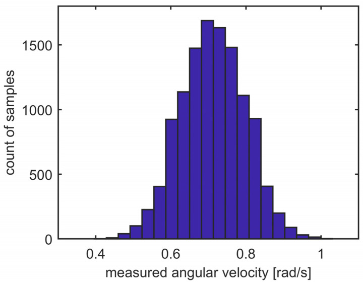
where r is the sensor’s resolution in bits (e.g., r = 16 bits for the MPU9250 sensor). The histogram of the real gyroscope noise is shown in Figure 1.
Figure 1.
Histogram of the sensor noise.
Since the gyroscope is a directional sensor (measures angular velocity around one or multiple principal perpendicular axes), the misalignment of the sensor is a source of the systematic error:
| (5) |
where ε is the misalignment angle. In the case of three-dimensional movements, the misalignment causes cross-talk between axes, which is expressed by the rotational matrix Ralign:
| (6) |
Another source of systematic errors is the miscalibration of the sensor—deviation of its gain and/or offset:
| (7) |
where G is the gain and B is the bias. The gain and bias are generally unpredictable and vary with time and temperature. The MEMS gyroscope measures the Coriolis force affecting periodically oscillating mass. Vibrations of the measured object perpendicular to the sensing axis of the gyroscope may cause additional periodic components of the measured signal due to the resonance. Such disturbance can be modeled using discrete Fourier series. It is a sum of harmonic (sinus) signals with frequencies from 0 to Nyquist frequency . The smallest frequency change detectable by the sensor with the constant sampling frequency is , where is the count of samples (window size). The model of the periodic noise is then:
| (8) |
where A is the amplitude of the measured oscillations (not to be confused with the amplitude of the vibrations itself), Ts is the sampling period of the sensor, and φ is the phase of the measured oscillations. Altogether, the measured value at the output of the single-axis gyroscope is:
| (9) |
If we use the sensor with sufficient full-scale range and a very small quantization step , the model of the sensor can be considered linear. The mean square error of the estimated angular velocity is:
| (10) |
where is the directional gain of the sensor. Since we assume that the internal noise component is independent from the true value , the mean of their product is negligible. At zero rate (during static calibration, ), the output bias B can be observed at the output of the gyroscope as the mean value, and the MSE is:
| (11) |
The same principles and formulas are valid for accelerometers or any sensors sensitive to the environmental noise.
2.3. Synchronization Errors
Within a multi-sensor environment, we need to consider the synchronization of individual sensors. Some intelligent sensors provide a trigger input, which allows the master controller (e.g., a microprocessor) to send a synchronization pulse, starting the measurement of all sensors at the same time. To quantify the impact of incorrect synchronization, we may assume two identical sensors with the same sampling period Ts but with different sampling phases. Qualitatively, the effect of invalid synchronization increases when the measured variable changes rapidly. If we model the dynamic input signal (true measured angular velocity) as a sine wave with the frequency fsig, the readings of two sensors are:
| (12) |
| (13) |
where A is the signal amplitude, is white Gaussian noise superposed independently to both sensors, and τ is the synchronization delay of the second sensor. Naïve sensor fusion is the average of the two sensors:
| (14) |
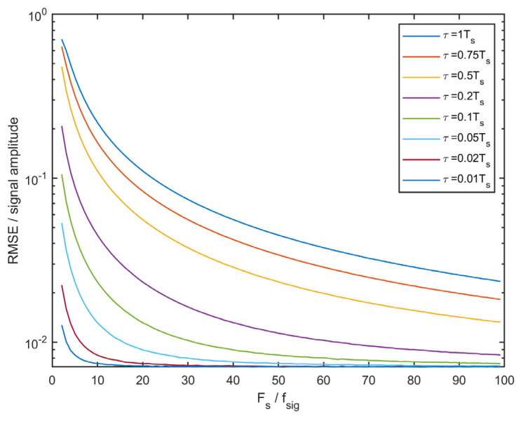
Figure 2 shows the RMSE of the value estimated using equation (14 concerning the relative sampling frequency and synchronization delay. The RMSE of each sensor noise was set to 1% of the signal amplitude for the simulation. A significantly larger sampling frequency than signal frequency (20 times and more) suppresses the adverse effects of invalid sensor synchronization (note the logarithmic vertical scale).
Figure 2.
RMSE of the sensor fusion concerning the sampling frequency and synchronization delay between two identical sensors.
3. Homogeneous Sensor Fusion
We may now analyze the situation when multiple almost-identical sensors sense the same variable. While the environmental noise (e.g., vibrations) is common for all sensors, the random internal sensor noise is purely random. The homogeneous sensor fusion can be expressed as a weighted average of the sensors’ readings:
| (15) |
where qj is the weight of the j-th sensor. If we apply Equations (9)–(15), neglecting the quantization and limits of the sensor, we obtain:
| (16) |
The goal of the sensor fusion is to minimize the MSE of the output (least-squares method). Theoretically, if the gain and bias errors are completely compensated by calibration, the sensor is perfectly aligned, and there are no vibrations present, the only source of the error is the internal noise of the sensor, and the result of the sensor fusion is:
| (17) |
The MSE of the sensor fusion is then:
| (18) |
When each ideal sensor has a weight coefficient proportional to , the MSE of the ideal sensor fusion result MSE(Ωideal) will be minimal (see, e.g., [28]).
| (19) |
The precision of the real fusion result depends on the precise estimation of the MSE. If we use the zero-rate estimate of the MSE (Equation (11)), which is an overestimate, the MSE of the sensor fusion result will be worse. We do not know the harmonic components of the measured vibrations (parameters Am, φm), nor the values of the calibration parameters after a longer run. The values of the calibration parameters for a group of sensors are considered randomly distributed around their ideal values. When the homogeneous sensor fusion (weighted average) provides a reasonable estimate of the true value, it is possible to estimate the values of the calibration parameters from the last N samples. The simple calibration model is:
| (20) |
where is the k-th raw digital sample of the j-th sensor converted to SI units, is the corresponding calibrated value, and are the calibration parameters. The Equation (20) represents the first-order (linear) calibration model. The sensor gain should ideally be equal to one; the c1 parameter represents gain deviation and is usually significantly lower than one. The form of the calibration model was chosen to improve numerical precision when floating point numbers are used. The calibration parameters c1 and c2 may be considered quasi-constant since they may slightly vary with the elapsed time and temperature. In the ideal case, both calibration parameters are zero. If we invert (20) and compare it with (7), the gain and bias of j-th sensor Gj, Bj from (7) can be rewritten in terms of c1j, c2j:
| (21) |
| (22) |
If we would know the true value and the noise is Gaussian, the calibration parameters can be estimated using the least-squares method:
| (23) |
| (24) |
In a real application, the true value is unknown. In the case of multiple sensors, the apriori estimate of the true value is the mean of all calibrated sensors’ measurements at the given time (all qj are the same):
| (25) |
where M is the count of sensors. Initially, the bias and gain deviation may be set to zero; hence, .
Algorithm 1 explains the homogeneous sensor fusion with the calibration estimation:
| Algorithm 1 Homogeneous sensor fusion with calibration |
| set: for j = 1 to M get end for initialize the estimate of the true value: compute sensor deviation compute the calibration parameters c1, c2 using (24) for j = 1 to M compute calibrated values end for for r = 1 to iterations re-compute the estimate of the true value: for j = 1 to M compute the MSE of each sensor compute the weight of the sensor end for compute maximal weight , truncation factor µ = 3 (empirical) for j = 1 to M truncate normalize: end for end for |
In the real-time version of the above algorithm, we process a fixed-size window of historical raw readings.
Truncation Factor
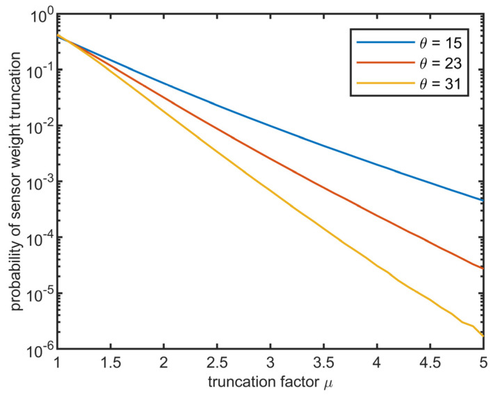
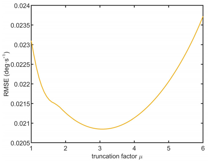
The proposed algorithm has intrinsic instability. When the MSE of one sensor is significantly underestimated compared to the other sensors, the estimated MSE of that sensor is low and its weight qj is significantly higher than the weights of the other sensors. Such a sensor becomes a “dictator”—in the next iteration, the estimated weighted average is pulled towards the readings of the dictator sensor. Therefore, it is pulled away from the readings of the other sensors. Then, the algorithm overestimates the MSE of the other sensors, resulting in a further decrease in their weight. After multiple iterations, the normalized weight of the dictator sensor converges to one, and all other sensors are suppressed. To avoid such behavior, truncation factor µ was introduced. It ensures that the weight of the best sensor never exceeds µ-times the average weight of all sensors. Suppose we assume that the RMS of a single sensor is a gamma-distributed random variable. In that case, the probability of false truncation (underestimation of the best sensor) is shown in Figure 3. The parameter shape θ = 23 ± 8 (std. deviation) and scale β = 0.03 ± 0.01 of the gamma distribution were roughly estimated by fitting the histogram of the RMS values obtained from a sample of 16 sensors. Figure 4 shows the RMSE of the estimated angular velocity concerning the truncation factor (see the next section for further details about the simulation parameters). According to the simulation results, the optimal truncation factor is approximately 3, which is the value to be used for further experiments. The false sensor weight truncation probability for μ = 3 is around 1%.
Figure 3.
Simulated probability of the false sensor weight truncation using the scale factor of the gamma distribution with the shape θ = 23 ± 8 and scale β = 0.82/θ.
Figure 4.
RMS error of the estimated angular velocity vs. truncation factor.
4. Simulation
We have used both simulation and real experiments to test the proposed method’s performance. The simulation raw data were computed using MATLAB R2021a environment with the following parameters:
count of the samples N = 10,000
sampling frequency FS = 100 Hz
amplitude of the random signal A = 200 deg·s−1
frequency vector of the random signal f[k] = 1.0 Hz + ξ, where ξ is normally distributed random number (implemented by MATLAB function randn)
phase of the random signal (implemented as MATLAB function cumsum)
simulated (true) angular velocity:
RMS of all 16 sensors is from a gamma distribution with shape α = 5 and scale β = 0.02
bias of all 16 sensors is from a zero-centered Gaussian distribution with standard deviation σ = 30 deg·s−1
gain of all 16 sensors is one-centered with standard deviation σ = 0.04
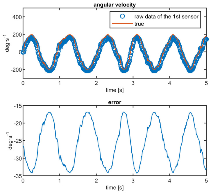
The above parameters roughly correspond to the noise parameters of real low-cost MEMS gyroscopes available commercially. Using a pseudo-sinusoidal signal with a fluctuating frequency simulates the continuous angular velocity of a physical object with a non-zero moment of inertia. An example of the simulated signal is in Figure 5. The average gain across all sensors equals one and the average bias is zero. Such normalization is necessary because the algorithm cannot intuitively determine the common-cause bias of all sensors without any apriori information (e.g., from different types of sensors). For simplicity, when all sensors deviate in the same direction, the result will also deviate in that direction.
Figure 5.
Simulated angular velocity.
5. Simulation Results
In the simulation mode, each sensor’s gain, bias, and MSE are known. Therefore, we may compute the optimal weights and compare the estimated parameters with the known values (see Table 1).
Table 1.
Convergence of simulation.
| Sensor No. j | Gain Gj (-) | Bias Bj (deg·s−1) | RMSj (deg·s−1) | |||
|---|---|---|---|---|---|---|
| Estimated | True | Estimated | True | Estimated | True | |
| 1 | 0.956946 | 0.956949 | −25.5111 | −25.5107 | 0.103 | 0.101 |
| 2 | 0.998366 | 0.998368 | −8.0970 | −8.0975 | 0.097 | 0.099 |
| 3 | 0.963520 | 0.963516 | −13.9765 | −13.9773 | 0.077 | 0.077 |
| 4 | 1.016634 | 1.016636 | 6.7336 | 6.7339 | 0.085 | 0.088 |
| 5 | 0.990664 | 0.990654 | 34.6136 | 34.6141 | 0.163 | 0.162 |
| 6 | 0.963372 | 0.963376 | −6.1223 | −6.1218 | 0.049 | 0.053 |
| 7 | 0.990176 | 0.990172 | 46.9899 | 46.9911 | 0.147 | 0.147 |
| 8 | 0.987289 | 0.987301 | 15.0531 | 15.0539 | 0.101 | 0.102 |
| 9 | 1.008443 | 1.008421 | −81.3185 | −81.3222 | 0.198 | 0.204 |
| 10 | 1.053295 | 1.053302 | −23.8845 | −23.8849 | 0.094 | 0.101 |
| 11 | 1.003599 | 1.003604 | 45.7136 | 45.7147 | 0.076 | 0.079 |
| 12 | 0.996136 | 0.996143 | −33.4840 | −33.4843 | 0.055 | 0.060 |
| 13 | 1.056180 | 1.056180 | 11.0308 | 11.0311 | 0.064 | 0.070 |
| 14 | 0.988030 | 0.988037 | −0.2502 | −0.2506 | 0.123 | 0.122 |
| 15 | 0.972770 | 0.972752 | 2.3391 | 2.3411 | 0.177 | 0.173 |
| 16 | 1.054589 | 1.054589 | 30.1703 | 30.1694 | 0.072 | 0.078 |
The algorithm converges under the abovementioned ideal conditions (zero-centered biases, one-centered gains). The shown values are obtained by three iterations of the RMS estimation. Please note that the algorithm, as described, computes MSE (mean square error) instead of RMS to avoid unnecessary computation of the square root.
6. Experimental Setup
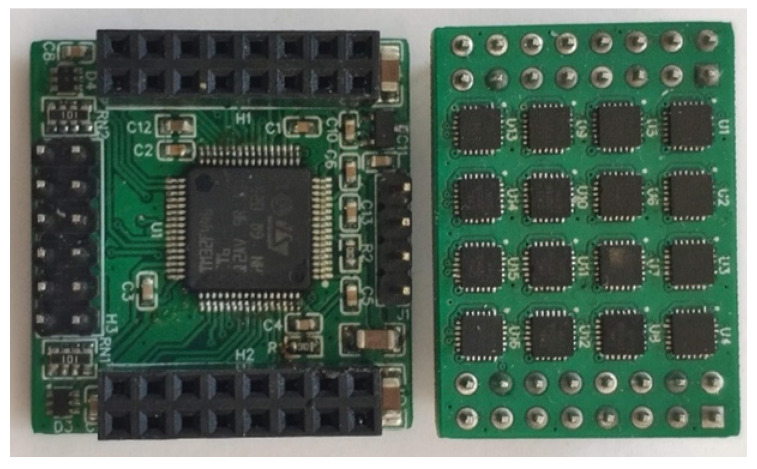
Real-world experiments were conducted using a matrix of 16 MPU9250 MEMS sensors from TDK InvenSense (Shenzhen, China) (see Figure 6). All sensors communicate with the microcontroller STM32F446 from STMicroelectronics (Geneva, Switzerland) via two independent SPI channels. The microcontroller then sends all sensor readings to the computer via serial connection. To synchronize the sensor readings, all sensors contain synchronization trigger input. The synchronized readings are stored within internal FIFO buffers within each sensor and later retrieved via SPI. The typical noise characteristics of the used gyroscope sensor obtained from the datasheet are [29]:
gain tolerance ±3% (at 25 °C), ±4% (whole temperature range −40 °C to +85 °C)
nonlinearity ±0.1%
bias tolerance ±5 deg·s−1 (at 25 °C), ±30 deg·s−1 (whole temperature range from −40 °C to +85 °C)
RMS noise 0.1 deg·s−1
Figure 6.
Sensor matrix (right) and microcontroller module (left).
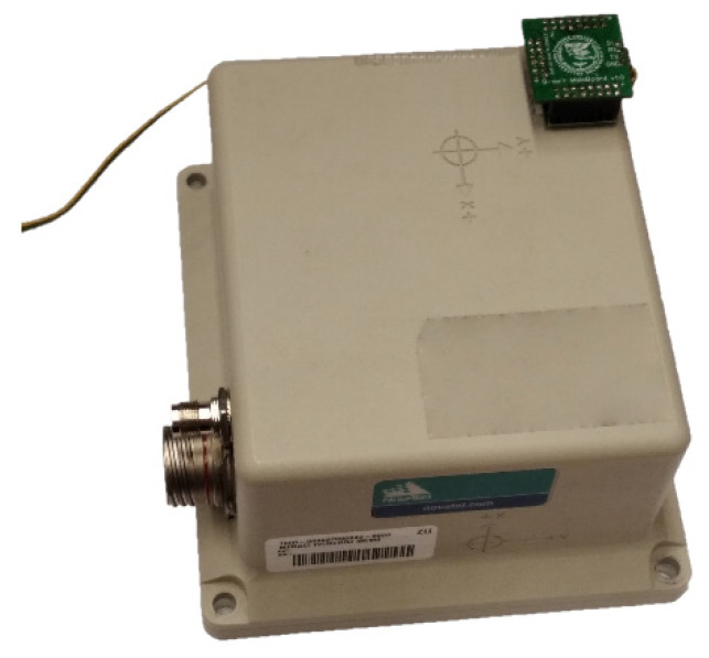
To evaluate the proposed method, it is necessary to measure the ground-truth value of the angular velocity. Our first attempts utilized a stepper motor driving a rotational platform. Still, the MEMS gyroscopes mentioned above captured the high-frequency changes in the motor’s rotation speed caused by the steps. The frequency of those steps is higher than the Nyquist frequency of the sensors, thus causing aliasing. To circumvent that, we attached the sensor matrix to a commercially available SPAN-CPT inertial navigation unit from NovTel Inc. (Calgary, AB, Canada), which contains three DSP-3000 single axial fiber optical gyroscopes (FOGs) manufactured by KVH Industries (Middletown, CT, USA). The characteristics of FOG sensors are [30]:
sampling frequency: 1000 Hz (downsampled by SPAN-CPT to 100 Hz)
initial bias: ±20°/h
nonlinearity: 500 ppm at ±150°/h
bias stability: 1°/h
angle random walk: 0.067°/√h
RMS (measured): 0.005°/s
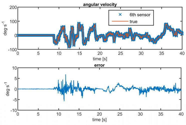
It is clear that FOG has 20 times lower RMS, so it thus may be used as a source of ground-truth value. Initial calibration allows us to compensate for the bias of the FOG sensor. The matrix of MEMS sensors attached to the SPAN-CPT unit is shown in Figure 7. Both sensors were rotated randomly by hand. The time series of the measured angular velocity from the MEMS array and FOG was roughly synchronized using a timestamp and fine-aligned by hand to suppress delays caused by the communication interfaces in the PC. The manual alignment of MEMS and FOG signals is needed only for validation purposes; in real applications, the FOG is not present. The measured angular velocity is in Figure 8.
Figure 7.
MEMS sensor array mounted at the top of the FOG unit.
Figure 8.
Comparison between 6th MEMS gyroscope and true value from FOG.
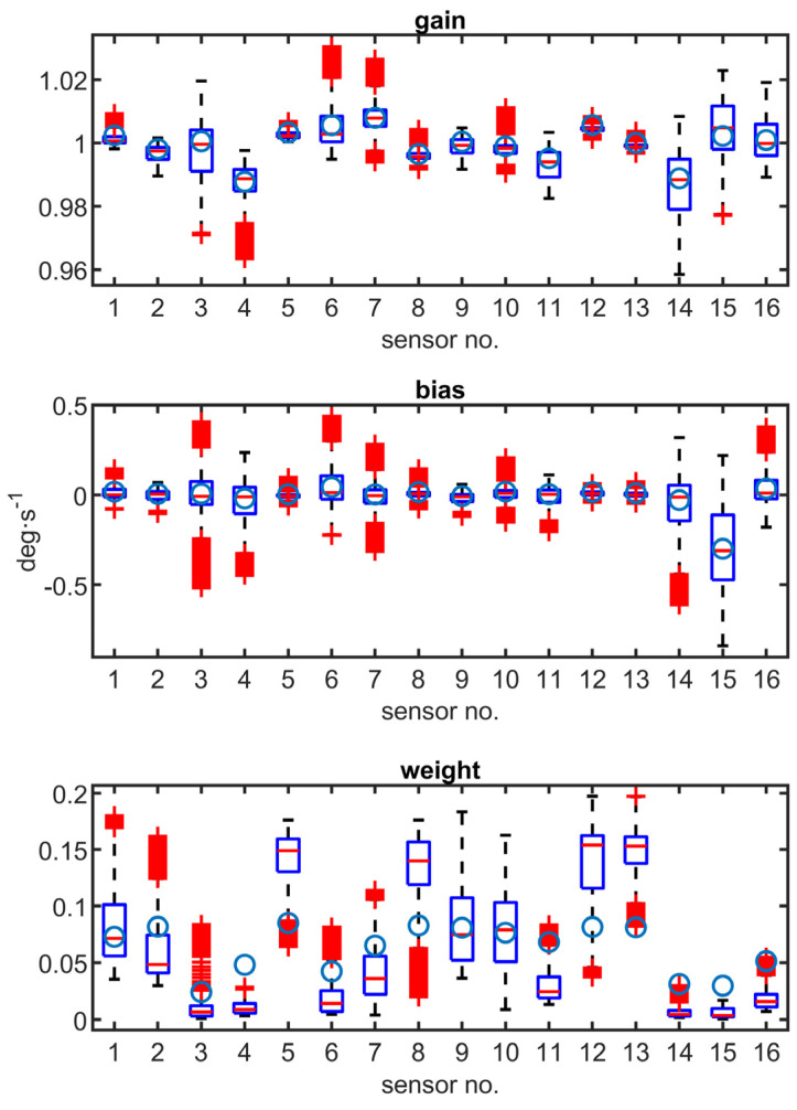
The estimated gain, bias, and weight of all sensors are shown in Figure 9, which presents a comparison of the sensor calibration parameters. Blue circles are “true” values considering the FOG data. The results are obtained using a moving window with the size of 1000 samples (processing the last 10 s). Shown outliers represent short-term calibration changes.
Figure 9.
Comparison of sensors’ calibration parameters. Blue circles are “true” values considering the FOG data.
As seen in Table 2 and Figure 9, the bias and gain of sensors were estimated correctly. The true gain and bias were obtained by comparing the results of the MEMS sensor with the readings from FOG. Those reference values lay within bounding boxes of estimated gain and bias. The mean absolute error of the gain estimation was 0.46%, and the mean absolute error of the bias estimation was 0.04 deg·s−1 (0.016% of the gyroscope full scale). The weights of the sensors are estimated roughly, with a mean absolute error of 41%, but it reflects the qualitative difference between the sensors (e.g., sensors j = 3, 4, 14, 15 have low weights). Table 3 compares two scenarios: the first with the real measured data and the second with an artificial white Gaussian noise added to one of the sensors, which emulates the degradation.
Table 2.
Estimated parameters of individual sensors.
| Sensor No. j | Gain Gj (-) | Bias Bj (deg·s−1) | Weight qj (-) | |||
|---|---|---|---|---|---|---|
| Estimated | True | Estimated | True | Estimated | Optimal | |
| 1 | 0.9986 | 1.0024 | −0.0026 | 0.0176 | 0.0580 | 0.0726 |
| 2 | 1.0007 | 0.9981 | 0.0044 | 0.0064 | 0.0407 | 0.0816 |
| 3 | 1.0019 | 1.0005 | −0.0092 | 0.0065 | 0.0836 | 0.0241 |
| 4 | 0.9957 | 0.9878 | −0.0110 | −0.0195 | 0.0149 | 0.0480 |
| 5 | 1.0018 | 1.0033 | −0.0068 | 0.0038 | 0.0912 | 0.0849 |
| 6 | 0.9957 | 1.0056 | 0.0132 | 0.0437 | 0.0808 | 0.0422 |
| 7 | 1.0106 | 1.0079 | −0.0042 | 0.0028 | 0.1075 | 0.0649 |
| 8 | 0.9956 | 0.9965 | 0.0134 | 0.0160 | 0.1190 | 0.0827 |
| 9 | 1.0022 | 1.0004 | −0.0096 | −0.0064 | 0.0850 | 0.0807 |
| 10 | 0.9991 | 0.9989 | 0.0115 | 0.0183 | 0.0561 | 0.0762 |
| 11 | 0.9975 | 0.9951 | 0.0120 | 0.0044 | 0.0828 | 0.0679 |
| 12 | 1.0041 | 1.0056 | −0.0011 | 0.0161 | 0.0377 | 0.0813 |
| 13 | 0.9981 | 1.0000 | −0.0001 | 0.0102 | 0.0820 | 0.0810 |
| 14 | 0.9999 | 0.9888 | −0.0125 | −0.0289 | 0.0291 | 0.0311 |
| 15 | 1.0172 | 1.0022 | −0.7651 | −0.2994 | 0.0021 | 0.0297 |
| 16 | 0.9927 | 1.0009 | 0.0098 | 0.0349 | 0.0297 | 0.0511 |
Table 3.
Comparison of results.
| Constellation | RMSE (deg·s−1) | |
|---|---|---|
| Measured Data | Single Sensor Additive Noise | |
| Single sensor | 0.945 | 10.000 |
| The mean of 16 sensors, no calibration | 0.720 | 0.936 |
| The mean of 16 sensors, with calibration | 0.701 | 0.924 |
| The weighted sum of 16 sensors, with calibration | 0.685 | 0.688 |
7. Conclusions
This article deals with the real-time calibration and sensor fusion in the homogeneous sensor array of the MEMS gyroscopes, measuring the angular velocity. The proposed method has been validated by both simulation and real-world experiments. The results of the experiments show that the algorithm improves the precision of the estimated angular velocity by approx. 5% compared to a naïve average when all sensors are working. The main advantage of the algorithm is the intrinsic ability to compensate for the degradation of some sensors using an adaptive weighted average, thus improving the reliability of the sensor array. The homogeneous sensor fusion can estimate calibration parameters (gain, bias) of individual sensors within the sensor array without the need for precise offline calibration equipment. Compared to the LVM (linear minimum variance) methods, our method does not require apriori information about error covariance matrices for individual sensors and can capture the changes in the error characteristics in real time. The proposed method applies to all types of sensors (not exclusively MEMS gyroscopes) because it does not require additional information. One of the critical challenges in such a configuration is to keep sensors in sync, which can be achieved by a global synchronization signal routed to all sensors. This drawback can be neglected when the sampling period is significantly smaller than the time constant of the system dynamics.
Author Contributions
Conceptualization, D.N.; methodology, D.N.; software, J.A.; validation, V.S.; formal analysis, D.N.; resources, J.H. All authors have read and agreed to the published version of the manuscript.
Institutional Review Board Statement
Not applicable.
Informed Consent Statement
Not applicable.
Data Availability Statement
All data associated with the article are available online at https://github.com/dusan-nemec/mems-calib (accessed on 10 May 2023).
Conflicts of Interest
The authors declare no conflict of interest.
Funding Statement
This research was funded by VEGA, grant number 1/0241/22: Mobile robotic systems for support during crisis situations.
Footnotes
Disclaimer/Publisher’s Note: The statements, opinions and data contained in all publications are solely those of the individual author(s) and contributor(s) and not of MDPI and/or the editor(s). MDPI and/or the editor(s) disclaim responsibility for any injury to people or property resulting from any ideas, methods, instructions or products referred to in the content.
References
- 1.Batista P., Silvestre C., Oliveira P., Cardeira B. Accelerometer calibration and dynamic bias and gravity estimation: Analysis design and experimental evaluation. IEEE Trans. Control Syst. Technol. 2011;19:1128–1137. doi: 10.1109/TCST.2010.2076321. [DOI] [Google Scholar]
- 2.Ruzza G., Guerriero L., Revellino P., Guadagno F.M. Thermal compensation of low-cost MEMS accelerometers for tilt measurements. Sensors. 2018;18:2536. doi: 10.3390/s18082536. [DOI] [PMC free article] [PubMed] [Google Scholar]
- 3.Engelsman D., Klein I. A Learning-Based Approach for Bias Elimination in Low-Cost Gyroscopes; Proceedings of the 2022 IEEE International Symposium on Robotic and Sensors Environments (ROSE); Abu Dhabi, United Arab Emirates. 14–15 November 2022; pp. 01–05. [DOI] [Google Scholar]
- 4.Wang P., Li Q., Zhang Y., Xi X., Wu Y., Wu X., Xiao D. Scale Factor Self-Calibration of MEMS Gyroscopes Based on the High-Order Harmonic Extraction in Nonlinear Detection. IEEE Sens. J. 2022;22:21761–21768. doi: 10.1109/JSEN.2022.3210723. [DOI] [Google Scholar]
- 5.Belkhouche F. Robust Calibration of MEMS Accelerometers in the Presence of Outliers. IEEE Sens. J. 2022;22:9500–9508. doi: 10.1109/JSEN.2022.3163964. [DOI] [Google Scholar]
- 6.Hu P., Chen B., Zhang C., Wu Q. Correlation-Averaging Methods and Kalman Filter Based Parameter Identification for a Rotational Inertial Navigation System. IEEE Trans. Ind. Inform. 2019;15:1321–1328. doi: 10.1109/TII.2018.2850756. [DOI] [Google Scholar]
- 7.Xie S., Abarca A., Markenhof J., Ge X., Theuwissen A. Analysis and calibration of process variations for an array of temperature sensors; Proceedings of the 2017 IEEE SENSORS; Glasgow, UK. 29 October–1 November 2017; pp. 1–3. [DOI] [Google Scholar]
- 8.Wang L., Tang H., Zhang T., Chen Q., Shi J., Niu X. Improving the Navigation Performance of the MEMS IMU Array by Precise Calibration. IEEE Sens. J. 2021;21:26050–26058. doi: 10.1109/JSEN.2021.3118455. [DOI] [Google Scholar]
- 9.Olsson F., Kok M., Halvorsen K., Schön T.B. Accelerometer calibration using sensor fusion with a gyroscope; Proceedings of the 2016 IEEE Statistical Signal Processing Workshop (SSP); Palma de Mallorca, Spain. 26–29 June 2016; pp. 1–5. [DOI] [Google Scholar]
- 10.Wang P., Li G., Gao Y. A Compensation Method for Random Error of Gyroscopes Based on Support Vector Machine and Beetle Antennae Search Algorithm; Proceedings of the 2021 International Conference on Computer, Control and Robotics (ICCCR); Shanghai, China. 8–10 January 2021; pp. 283–287. [DOI] [Google Scholar]
- 11.Shen C., Zhang Y., Guo X., Chen X., Cao H., Tang J., Li J., Liu J. Seamless GPS/Inertial Navigation System Based on Self-Learning Square-Root Cubature Kalman Filter. IEEE Trans. Ind. Electron. 2021;68:499–508. doi: 10.1109/TIE.2020.2967671. [DOI] [Google Scholar]
- 12.Jiang P., Liang H., Li H., Dong S., Wang H. Online Calibration Method of Gyro Constant Drift for Low-Cost Integrated Navigator; Proceedings of the 2019 5th International Conference on Control, Automation and Robotics (ICCAR); Beijing, China. 19–22 April 2019; pp. 846–850. [DOI] [Google Scholar]
- 13.Huttner F., Kalkkuhl J., Reger J. Offset and Misalignment Estimation for the Online Calibration of an MEMS-IMU Using FIR-Filter Modulating Functions; Proceedings of the 2018 IEEE Conference on Control Technology and Applications (CCTA); Copenhagen, Denmark. 21–24 August 2018; pp. 1427–1433. [DOI] [Google Scholar]
- 14.Ma J., Xu H., Li C., He F., Liang Y. Research of high precision quartz temperature sensor system based on data fusion technology; Proceedings of the 2013 2nd International Conference on Measurement, Information and Control; Harbin, China. 16–18 August 2013; pp. 1051–1054. [DOI] [Google Scholar]
- 15.Alteriis G.d., Accardo D., Lo Moriello R.S., Ruggiero R., Angrisani L. Redundant configuration of low-cost inertial sensors for advanced navigation of small unmanned aerial systems; Proceedings of the 2019 IEEE 5th International Workshop on Metrology for AeroSpace (MetroAeroSpace); Turin, Italy. 19–21 June 2019; pp. 672–676. [DOI] [Google Scholar]
- 16.Napieralski J.A., Tylman W. Multi-sensor Data Fusion for Object Rotation Estimation; Proceedings of the 2018 25th International Conference “Mixed Design of Integrated Circuits and System” (MIXDES); Gdynia, Poland. 21–23 June 2018; pp. 454–459. [DOI] [Google Scholar]
- 17.Guan Y., Song X. Sensor Fusion of Gyroscope and Accelerometer for Low-Cost Attitude Determination System; Proceedings of the 2018 Chinese Automation Congress (CAC); Xi’an, China. 30 November–2 December 2018; pp. 1068–1072. [DOI] [Google Scholar]
- 18.Webber M., Rojas R.F. Human Activity Recognition With Accelerometer and Gyroscope: A Data Fusion Approach. IEEE Sens. J. 2021;21:16979–16989. doi: 10.1109/JSEN.2021.3079883. [DOI] [Google Scholar]
- 19.Contreras-Rodriguez L.A., Muñoz-Guerrero R., Barraza-Madrigal J.A. Algorithm for estimating the orientation of an object in 3D space, through the optimal fusion of gyroscope and accelerometer information; Proceedings of the 2017 14th International Conference on Electrical Engineering, Computing Science and Automatic Control (CCE); Mexico City, Mexico. 20–22 October 2017; pp. 1–5. [DOI] [Google Scholar]
- 20.Peniak P., Rástočný K., Kanáliková A., Bubeníková E. Simulation of Virtual Redundant Sensor Models for Safety-Related Applications. Sensors. 2022;22:778. doi: 10.3390/s22030778. [DOI] [PMC free article] [PubMed] [Google Scholar]
- 21.Ždánsky J., Rástočný K., Medvedík M. Safety of Two-Channel Connection of Sensors to Safety PLC; Proceedings of the 2020 ELEKTRO; Taormina, Italy. 25–28 May 2020; pp. 1–5. [DOI] [Google Scholar]
- 22.Do H.V., Kwon Y.S., Kim H.J., Song J.W. An Improvement of 3D DR/INS/GNSS Integrated System using Inequality Constrained EKF; Proceedings of the 2022 22nd International Conference on Control, Automation and Systems (ICCAS); Jeju, Republic of Korea. 27 November–1 December 2022; pp. 1780–1783. [DOI] [Google Scholar]
- 23.Yang K., Liu M., Xie Y., Zhang X., Wang W., Gou S., Su H. Research on UWB/IMU location fusion algorithm based on GA-BP neural network; Proceedings of the 2021 40th Chinese Control Conference (CCC); Shanghai, China. 26–28 July 2021; pp. 8111–8116. [DOI] [Google Scholar]
- 24.Ye H., Chen Y., Liu M. Tightly Coupled 3D Lidar Inertial Odometry and Mapping; Proceedings of the 2019 International Conference on Robotics and Automation (ICRA); Montreal, QC, Canada. 20–24 May 2019; pp. 3144–3150. [DOI] [Google Scholar]
- 25.Yao Y., Xu X., Li Y., Zhang T. A Hybrid IMM Based INS/DVL Integration Solution for Underwater Vehicles. IEEE Trans. Veh. Technol. 2019;68:5459–5470. doi: 10.1109/TVT.2019.2910397. [DOI] [Google Scholar]
- 26.Zhu Y., Li X., Zhao J. Linear minimum variance estimation fusion. Sci. China Ser. F. 2004;47:728–740. doi: 10.1360/03yf0087. [DOI] [Google Scholar]
- 27.Carlsson H., Skog I., Jaldén J. Self-Calibration of Inertial Sensor Arrays. IEEE Sens. J. 2021;21:8451–8463. doi: 10.1109/JSEN.2021.3050010. [DOI] [Google Scholar]
- 28.Nemec D., Šimák V., Janota A., Hruboš M., Bubeníková E. Precise localization of the mobile wheeled robot using sensor fusion of odometry, visual artificial landmarks and inertial sensors. Robot. Auton. Syst. 2019;112:168–177. doi: 10.1016/j.robot.2018.11.019. [DOI] [Google Scholar]
- 29.InvenSense MPU-9250 Product Summary. 2015. [(accessed on 1 February 2023)]. Datasheet. Available online: https://invensense.tdk.com/wp-content/uploads/2015/02/PS-MPU-9250A-01-v1.1.pdf.
- 30.KVH Industries, Inc. DSP-3000 FOG, High-Performance, Single-Axis Fiber Optic Gyro. [(accessed on 1 February 2023)]. Datasheet. Available online: http://www.canalgeomatics.com/wp-content/uploads/2019/11/kvh-dsp-3000-fog-datasheet.pdf.
Associated Data
This section collects any data citations, data availability statements, or supplementary materials included in this article.
Data Availability Statement
All data associated with the article are available online at https://github.com/dusan-nemec/mems-calib (accessed on 10 May 2023).


