

Abstract
Motivation
With the rapid development of modern technologies, massive data are available for the systematic study of Alzheimer’s disease (AD). Though many existing AD studies mainly focus on single-modality omics data, multi-omics datasets can provide a more comprehensive understanding of AD. To bridge this gap, we proposed a novel structural Bayesian factor analysis framework (SBFA) to extract the information shared by multi-omics data through the aggregation of genotyping data, gene expression data, neuroimaging phenotypes and prior biological network knowledge. Our approach can extract common information shared by different modalities and encourage biologically related features to be selected, guiding future AD research in a biologically meaningful way.
Method
Our SBFA model decomposes the mean parameters of the data into a sparse factor loading matrix and a factor matrix, where the factor matrix represents the common information extracted from multi-omics and imaging data. Our framework is designed to incorporate prior biological network information. Our simulation study demonstrated that our proposed SBFA framework could achieve the best performance compared with the other state-of-the-art factor-analysis-based integrative analysis methods.
Results
We apply our proposed SBFA model together with several state-of-the-art factor analysis models to extract the latent common information from genotyping, gene expression and brain imaging data simultaneously from the ADNI biobank database. The latent information is then used to predict the functional activities questionnaire score, an important measurement for diagnosis of AD quantifying subjects’ abilities in daily life. Our SBFA model shows the best prediction performance compared with the other factor analysis models.
Availability
Code are publicly available at https://github.com/JingxuanBao/SBFA.
Contact
qlong@upenn.edu
Keywords: structural Bayesian factor analysis, multi-omics, Alzheimer’s disease, biological network
Introduction
With the rapid advances in modern biotechnologies such as high-throughput genotyping and sequencing, and multimodal neuroimaging, researchers can investigate disease mechanisms from multiple perspectives simultaneously. Multi-omics data integration enables us to discover new insights into biological mechanism of complex diseases such as cancer and Alzheimer’s disease (AD) [1].
AD diagnosis prediction or AD-related cognitive score prediction can help uncover novel therapeutic targets for AD. Many studies seek to predict the AD diagnosis or cognitive scores using only imaging data [2–8] or only genetics data [9]. However, due to the pathological heterogeneity of AD [10, 11], overly relying on one type of data may undermine the power of analyses. To boost the power of the existing AD research, studying AD from both imaging and genetics/genomics perspectives may improve prediction accuracy and reduce false negative signals [12–17]. In our study, we proposed a novel structural Bayesian factor analysis (SBFA) framework to extract the common information shared by both imaging and genetics/genomics information, which can be used to guide future AD research in a biologically meaningful way.
Factor analysis is a popular statistical method for integrative analysis of multi-modal data. The factor analysis aims to describe variability among high-dimensional variables in terms of a substantially lower number of unobserved variables called latent factors. Many state-of-the-art factor-analysis-based methods have been proposed and applied to multi-omics data [18], for example to integratively define the subtypes of diseases such as breast cancer [19–23] and lung cancer [19, 20]. The iCluster [19] is a widely used factor analysis framework based on the joint latent variable model. It can flexibly model different types of genomics data in a single framework. It successfully models the tumor subtypes as latent variables integrating the information from multiple datasets. Later, Mo et al. [24] extended the iCluster to the iCluster+ framework by allowing the simultaneous integration of continuous and discrete datasets. Another highly cited integrative factor analysis method based on the non-negative matrix factorization is joint and individual variation explained (JIVE) factor analysis [25], which extends iCluster by adding a data-specific term [21]. A recently published integrative factor analysis method, structural learning and integrative decomposition of multi-view data (SLIDE) [26], represents each data view via shared and individual components. SLIDE has been successfully applied to multiple applications including exploratory dimension reduction, association analysis and consensus clustering.
There has been limited work on integrative analysis of multi-omics and imaging data in a principled modeling framework in AD studies. Some existing AD studies applied factor analysis models trying to define AD subtypes solely in terms of neuropathology [27, 28], molecular signatures [29, 30] or solely through imaging phenotype [31, 32]. Additionally, none of these studies takes prior biological network information into consideration. Network information encourages the selection of related features (e.g. genes belonging to the same pathway) and produces a more biologically interpretable result.
In AD studies, the interactions or associations within or across molecular pathways can be treated as network information. Many databases can provide pathway-level interactions and associations such as Integrative Multi-species Prediction [33] and Kyoto Encyclopedia of Genes and Genomes [34–36]. Some databases can provide tissue-specific interactions and associations such as the HumanBase [37–40]. Several existing studies achieved the incorporation of the biological network information using network-based penalties [41, 42], or proper priors in the Bayesian statistics framework [43–46]. One factor-analysis-based Bayesian integrative study of multi-omics data proposed a generalized Bayesian factor analysis (GBFA) framework by extending the iCluster+ framework [47]. They incorporate the prior biological network information by employing the Markov random field prior. However, one limitation of the GBFA framework is the phase transition problem [48, 49], which may require a massive hyperparameter tuning process.
In this paper, we propose an SBFA model that assigns the Laplace prior to the loading matrix for feature selection. It also assigns a log-normal prior to the shrinkage parameter in the Laplace prior and assigns a graph Laplacian prior [50, 51] to the precision matrix in the log-normal prior. Our model formulation enables smoothing shrinkage parameters for variables that are connected in the biological graph. Our major contributions are summarized as follows:
We propose a novel structural Bayesian factor analysis framework as a dimension reduction technique that yields latent factors by integrating the genotyping data, gene expression data, region-level brain imaging amyloid deposition data and biological network information. Our SBFA framework is biologically interpretable. As such, the common information shared among multi-omics data learned from our model can be used for various subsequent analyses.
Our model can handle both continuous (e.g. gene expression and imaging phenotypic traits) and discrete [e.g. genotyping values for single nucleotide polymorphisms (SNPs)] data simultaneously. We successfully incorporate prior biological information without suffering the phase transition problem of the existing GBFA framework [47].
Our work bridges the gap that there are few multi-omics studies applied to AD. We extracted more biologically meaningful information from multiple modalities, and our framework achieves the best prediction accuracy for the subsequent machine learning prediction problems compared with the other state-of-the-art factor-analysis-based methods.
The rest of the paper is organized as follows. We introduce our proposed method including model formulation and computation in Section 2. We present and discuss the analyses of real data from the Alzheimer’s Disease Neuroimaging Initiative (ADNI) in Section 3. We present our simulation experiment results in Section 4 and conclude the paper with some discussion remarks in Section 5.
Methodology
We propose a hierarchical Structural Bayesian Factor Analysis model named SBFA (Figure 1). Our model serves as a dimension reduction technique to extract common information from multi-modal data.
Figure 1.
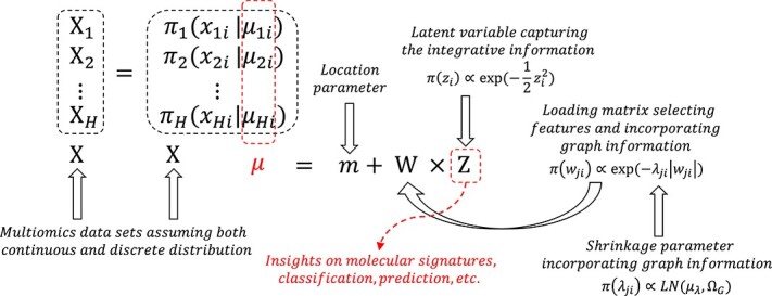
Structural Bayesian factor analysis framework.  represents the number of multi-modal data sets with each dataset denoted as
  ,
,  . The concatenation of all
  data sets is denoted by
  . We assume both continuous and discrete underlying distribution for each dataset dominated by mean parameter
  ,
,  where
where  is number of samples.
  represents the
  th column of factor matrix
  where
where  .
.  and
and  represent the
  th row and
  th column of loading matrix
  and shrinkage parameter for Laplacian prior where
  and
and  is the total number of features.
  represents the log-normal distribution.
  and
and  denote the mean and precision matrix for log-normal prior, respectively.
Notation
All vectors and matrices in this paper are denoted by bold lowercase letters or bold Greek letters. We use unbold lowercase letters or Greek letters to denote the corresponding elements of the vector/matrix. The columns and rows of the matrix are indicated by the subscription. For example,  where
where  denotes the
  th element of vector
  of length
  ;
;  where
where  and
and  denotes the element at the
  th row and
  th column of the matrix
  with dimension
  ;
;  represents the
  th column of matrix
  and the
  represents the
  th row of the matrix
  .
.
Structural Bayesian factor analysis model
Suppose we have multi-modal data with  modalities generated from
  different technologies. We denote each data modality by
  for
for  , where
  can be any omics data such as genotyping data, gene expression data, DNA methylation data and metabolomics data. Additionally, it can be imaging phenotypic traits such as brain gray matter density, brain volume, protein aggregates and metabolism level in a specific area of the brain. We denote the vertical concatenation of the multi-omics data to be
 |
where  and
and  is number of features in dataset
  ,
,  representing the
  th feature, and
  representing the
  th subject.
We assume that each feature of the dataset  has the same underlying distribution family
  governed by the mean parameter
  for each sample
  . Under the assumption that every subject is independent of each other and every omic dataset is independent of each other conditioning on
  , we can write the following likelihood function:
 |
Our SBFA framework can integrate multi-modal datasets with both continuous and discrete data types simultaneously, including Gaussian data, binomial data and negative binomial data.
-
Gaussian distribution:
Continuous is assumed to be normally distributed with mean
  and precision
  ,
,
where a gamma prior
 will be assigned to
  .
. -
Binomial distribution:
If the random variable follows a binomial distribution with parameters
  trials and success probability
we will use the logit model with probability mass function (pmf) shown as follows:
The parameter
(1)  is determined by data. Bernoulli distribution is a special case for the binomial distribution with
  to be 1.
 -
Negative binomial distribution:
To account for over-dispersion in counting data, we accommodate the negative binomial distribution
where parameter
(2)  is provided by data. The geometric distribution is a special case for the negative binomial distribution with
  to be 1.
The mean parameter  are modeled by the generalized factor analysis framework as
 |
which, in matrix form, can be written as follows:
 |
where  is the
  latent factor shared by all modalities;
  is the
  factor loading matrix;
  is the
  th row of
  and
and  is the
  th column of
  ;
;  , and
, and  . Our goal is to estimate a biologically meaningful low-rank representation (
 ) of
) of  to reduce the dimension of original multi-modal data while preserving the common information shared by multiple modalities. Such dimension reduction can reduce computational expenses and prevent the potential overfitting issue.
 represents a low-dimensional latent driver for all
  omics and imaging modalities and can be used for subsequent analysis in the applications on AD. For example, it can be used to cluster the subjects to define different AD subtypes. On the other hand, it can also serve as a predictor to predict the diagnosis-related cognitive traits such as the functional assessment questionnaire (FAQ) in the ADNI database, which will be described in Section 3.
Priors
Priors for W and Z
To obtain sparse estimates for  , we employ the Laplace prior for
 |
where  is the shrinkage parameter. The prior distributions for the entries in
  are the standard Gaussian distribution
 |
Prior for  : incorporating graphical knowledge
One key contribution of our work is to incorporate biological knowledge  via a structured prior for the shrinkage parameter
  . In our setting, the graph information for each omics dataset
  is represented by
  , where
  denotes the nodes and
  denotes the edges. The presence of an edge indicates that the corresponding pair of nodes are correlated. We denote the
  as the adjacency matrix representation of
  . We combine the
  to get the graph information for the multiomics data
  by diagonally concatenating the adjacency matrix for each omics data
  . Now, the graph information of multiomics data can be represented by
  where
where  with
with  and
and  with
with  referring to the index of the
  th feature of modality
  in the concatenated graph
  . Such a setup can help us to achieve the goal that given independent latent factors, the only way a pair of variables can be correlated conditionally on the rest is that they must load at least one common factor. Mathematically, if
  and
and  are connected in
  and
and  for some
  , then
  is encouraged to be nonzero. To this end, we employed a log-normal prior to
  with graph Laplacian on the precision matrix
 |
(3) |
where scalar  , the mean of
  , is a tuning parameter that controls the overall shrinkage level of
  . Scalar
  , variance of
  , controls the extent of individual shrinkage parameters
  adapted to
  and
and  . If
. If  , we have
  and the prior reduces to the Bayesian lasso. As
  increases,
  are more adapted to
  and
and  . In our study, we fix the relative variance, known as the adaptivity, to one to allow sufficient variability for
  for all shrinkage levels [47], i.e.
 |
or equivalently,
 |
The intuition behind the choice of log-normal prior is as follows: (i) we employ the log-normal distribution for  to incorporate the graph information via correlation and (ii) the shrinkage parameter
  needs to be positive.
Prior for  : incorporating biological knowledge
We use the graph Laplacian prior [45] for  to incorporate the graph information
  , which is a symmetric and diagonally dominant matrix
 |
where the elements in matrix  ,
,  , are assigned by the following prior:
 |
where  is the Dirac delta function concentrated at
  and
and  is the indicator function.
  represents all connected edges in prior biological graph information. In real data application, the graph information can be summarized from gene–gene interaction networks for genetics data and from brain functional pathway information for neuroimaging modality.
There are several mathematical intuitions behind the choice of  . First of all, the diagonal dominance of the precision matrix
  ensures its positive definiteness. Second, to ensure the positiveness of
  on the connected pairs, we incorporate a gamma-like distribution on all the connected pairs and
  on those pairs without an edge. The overall tendency of positiveness of the variance-covariance matrix ensures that increasing
  for some
  encourages an increase of the corresponding correlation.
Model for heterogeneous data types
Our model can handle heterogeneous data types simultaneously. In our framework, we use the exponential family for modeling heterogeneous data types in  . For example, gene expression and neuroimaging data can be modeled as continuous data with normal distribution. SNP data can be modeled as two Bernoulli random variables where each SNP feature can be represented by the presence of homozygous major allele and the presence of homozygous minor allele, respectively.
With three different underlying data distributions (Gaussian, binomial, negative binomial), we can integrate the discrete exponential family random variables by unifying the likelihood function via the following identity [52]:
 |
where  and
and  ( Pólya-Gamma distribution). By applying the identity to the binomial (Eq. (1)) and negative binomial (Eq. (2)) likelihood functions, we obtain the unified likelihood function:
 |
where the unknown parameters are shown in Table 1. Now, the full posterior density can be written as
Table 1.
Parameters for unified likelihood.
| Data Type |

|

|

|

|
|---|---|---|---|---|
| Gaussian |

|
0 | NA |

|
| Binomial | 0 |

|

|

|
| Negative Binomial | 0 |

|

|

|
 |
where  .
.
Feature representation
In our model, new feature representation is learned from genotyping, gene expression and imaging datasets with biological graph information. The high dimensional information is summarized into the low dimensional latent variable  for subsequent analyses.
For example, our SBFA framework estimated low dimensional latent features, which can serve as a predictor for machine learning algorithms. For unsupervised learning such as clustering, the low dimensional features derived from our algorithm are considered to be less noisy. We can apply the existing clustering algorithm to cluster the subjects based on the new feature representation. Supervised learning such as prediction often suffers from overfitting with high dimensional input data. With the low dimension feature representation derived from our algorithm, we can reduce the risk of overfitting. Compared with the other dimension reduction techniques, our SBFA is more biologically interpretable.
Parameter estimation and computation
We estimate the factor loading matrix  and the location parameter
  by finding the mode of their marginal posterior density, i.e. the maximum a posteriori (MAP) estimator. Specifically, denote the parameters to be estimated by
  and the nuisance parameters by
  . Then, the MAP estimator for
  and
and  is defined as
 |
where  is the (joint) posterior density. To find the MAP, we could utilize the expectation maximization (EM) algorithm [53], which iteratively maximizes conditional expectations as follows:
 |
where  denotes the expectation with respect to the conditional distribution
  .
.
Unfortunately, the conditional expectation of  in our model does not have a closed-form solution. Therefore, we choose to use the variational EM algorithm [54, 55], where the conditional distribution
  is approximated by a more tractable distribution family
  parameterized by
  . The variational parameter
  can be determined by minimizing the Kullback–Leibler (KL) divergence
 |
where  denotes the expectation under
  . Thus, the variational EM is equivalent to maximizing
 |
which is called the evidence lower bound (ELBO) [55] as it always satisfies  , with respect to
  and
and  .
.
In our model, we use a product measure on  as the variational (approximating) measure, i.e.
  where
where
 |
where  ’s,
’s,  ’s,
’s,  ’s
’s  ’s,
’s,  ’s,
’s,  ’s and
  ’s are variational parameters. Note that
  is called tilted Pólya-Gamma distribution.
E-step for  :
We update the variational parameters
:
We update the variational parameters  and
and  by matching the form of the equations between the expectation for log variational measure and the expectation for log posterior measure
 |
where  and
and  ;
;  is the mean of the variational measure for the
  th element of
  ;
;  is the
  th row and
  th column of the covariance matrix of the variational measure for
  .
.
We then update the expectation of the  using the mean formula for gamma distribution by
 |
for  and
and  . Now, we have a graph Laplacian matrix
 |
E-Step for  :
Since there exists an
:
Since there exists an  term in the log posterior distribution but not in the log variational measure, we cannot update the variational parameters by matching the form of equations as we did when updating the
  (E-step for
  ). Instead, we need to maximize the ELBO function and the results give us that
 |
where  ,
,  ,
,  represents the Lambert W function [56] and
 |
and  is an operator taking the diagonal elements of a square matrix as a column vector;
  represents the
  th row and
  th column element of the matrix
  ;
;  represents the mean matrix for
  ;
;  represents the covariance matrix for
  th column of
  ;
;  represents the
  th element of the vector
  .
.
The update rule for the covariance matrix of  , i.e.,
  , is separated into two parts. In the first part, we update the off-diagonal element of the
  by
by
 |
(4) |
for each  , where
 |
The  operator defines the trace of the matrix, and the minus sign in the subscript represents the matrix with the corresponding row or column removed, or vector with the corresponding element removed.
In the second part, we update the diagonal element of the  as follows:
 |
(5) |
for each  , where the r-Lambert function
  is defined as the inverse of the function
  [57] and
 |
where  is the inverse operator for a square matrix;
  is the
  th row and
  th column of the loading matrix
  . We iteratively update
  for each
  and
and  .
.
E-step for  :
We update the precision matrix of the
:
We update the precision matrix of the  th column of factor matrix
  , i.e.
  , by matching the form of equations between log posterior distribution and the log variational measure. For each
  , we have
 |
where  is identity matrix;
  is the mean for parameter
  and
and  is the
  th row of loading matrix
  . For each
  , we update the mean parameter for
  by
by
 |
E-step for  :
By matching the form of expectation of log posterior and expectation of log variational measure, the variational parameter
:
By matching the form of expectation of log posterior and expectation of log variational measure, the variational parameter  for each
  and
and  for
for  can be updated by
 |
where  is the
  th row of loading matrix
  and
and  is the variance-covariance matrix for variational measure of
  .
.
If  is a discrete random variable, we have
 |
whereas if  follows Gaussian distribution, we have
 |
M-step for  :
We update the loading matrix row by row via maximizing the ELBO function with respect to
:
We update the loading matrix row by row via maximizing the ELBO function with respect to  for each
  . The optimization problem is solved by the dynamic weighted lasso algorithm [58].
M-step for  :
The location parameter
:
The location parameter  is updated by maximizing the ELBO function with respect to
  for each
 |
Initialization
For the initialization, we define the matrix  as an approximation of the mean matrix
  as follows [47]:
 |
The location vector  can be initialized by a fixed pre-specified constant vector. If not, for each
  ,
,  can be initialized by the trimmed mean, median or mean of
  .
.
In our setting, we handle the problems by choosing  and
and  matrices close to orthogonal matrices via singular value decomposition. Specifically, we have
 |
where  and
and  are orthonormal matrices and
  is diagonal matrix.
Hyperparameter tunning
We used the Bayesian information criterion (BIC) to tune the hyperparameters. We select the hyperparameters with the lowest BIC criteria
 |
where  is the estimated mean matrix of
  ;
;  is the number of subjects and
  denotes the degrees of freedom, which is the number of non-zero elements in estimated factor loading matrix. We try different sets of hyperparameters (
 ) in both simulation and real data analysis.
Analysis of ADNI Data
To demonstrate the usefulness of our proposed method in real data analysis, we aimed to predict the FAQ cognitive score using the latent factors learned through integrative analysis of the genotyping, gene expression, brain regional level amyloid deposition, gene-gene interaction network and brain functional network data from the ADNI biobank database. We also performed the same analysis using existing factor analysis models (JIVE [25], SLIDE [26], iCluster+ [24], GBFA [47]) as the benchmark.
Data description and data preprocessing
The genotyping data, gene expression data, demographic data and imaging data used in the preparation of this article were obtained from the ADNI database (adni.loni.usc.edu) [59–61]. The ADNI was launched in 2003 as a public–private partnership, led by Principal Investigator Michael W. Weiner, MD. The primary goal of ADNI has been to test whether serial magnetic resonance imaging, positron emission tomography (PET), other biological markers and clinical and neuropsychological assessment can be combined to measure the progression of mild cognitive impairment (MCI) and early AD. Up-to-date information about the ADNI is available at www.adni-info.org.
After data preprocessing steps and the common subjects matching in each omics data, we have 604 subjects left with main characteristics summarized in Table 2.
Table 2.
Participant characteristics. Total number of subjects, age and sex are shown in this table. The mean  sd for the age of all subjects within each diagnosis group is reported. The number of male/female subjects within each diagnosis group is also shown.
| Diagnosis | CN | EMCI | LMCI | AD | Overall |
|---|---|---|---|---|---|
| Number | 199 | 198 | 165 | 42 | 604 |
Age ( ) ) |

|

|

|

|

|
| Sex (M/F) |

|

|

|

|

|
Demographic data preprocessing and cognitive score
Our demographic data and the cognitive score are extracted from Quantitative Templates for the Progression of Alzheimer’s Disease project in the Alzheimer’s Disease Modeling Challenge (www.pi4cs.org/qt-pad-challenge). We use baseline age, gender, education and the presence of APOE4 as our covariates. A test of the subjects’ daily living activities, the FAQ [62], is extracted as our dependent variable of real data analysis. All subjects with missing values are excluded from our study.
Genotyping data preprocessing
For the genotyping data, we performed quality control (QC) using the following criteria: genotyping call rate > 95%, minor allele frequency > 5% and Hardy–Weinberg Equilibrium >  . After the QC, rs429358 (APOE) SNP was added to the genotyping data. We prioritized the SNP markers based on the existing findings from the major AD GWAS articles [63–67]. Our raw data were obtained by additive recoding the number of minor alleles (–recode A in PLINK1.9 [68]). Given that we want to model our genotyping data as Bernoulli distribution, we further recoded the genotyping data by the presence of homozygous major allele and the presence of homozygous minor allele, which doubled the number of input features for the genotyping dataset.
Gene expression data preprocessing
Gene expression data were produced using Affymetrix Human Genome U219 Array (Affymetrix, Santa Clara, CA) for expression profiling where the blood sample extraction, hybridization and QC process could be found in [59]. In the raw data, one gene can correspond to multiple probes. In our real data analysis, we averaged all the probes within each gene across the subjects to obtain the corresponding gene expression. We prioritize the AD-related genes according to Disease Gene Network (DisGeNet) [69]. We extract all the genes that have gene–disease association scores [69] greater than 0.15.
Imaging data preprocessing
For the neuroimaging data, participants with complete [ F]florbetapir (AV45) PET data (measuring amyloid burden) were included in our analysis. The AV45 PET scans were registered to the Montreal Neurological Institute space, and the standard uptake value ratio was computed by intensity normalization using the cerebellar curs reference region. Region-of-interest-level (ROI-level) AV45 measures were extracted based on the Glasser atlas [70], where 360 ROI-level quantitative traits (QTs) were obtained by averaging all the voxel-level measures within each ROI.

Biological network
We download the tissue-specific gene–gene interaction network from GIANT [40] in HumanBase database (hb.flatironinstitute.org). The imaging network is obtained from Glasser et al. [70], which utilizes a supervised machine learning classifier to automatically delineate and identify each cortical area from its neighbors across a large majority of individual subjects based on multi-modal information.
Real data analysis
In our real data analysis, we evaluate our SBFA framework by predicting the FAQ score using our extracted latent factors, which can be considered as a low-dimensional representation of the multi-omics data sets. Our real data analysis pipeline is shown in Figure 2.
Figure 2.
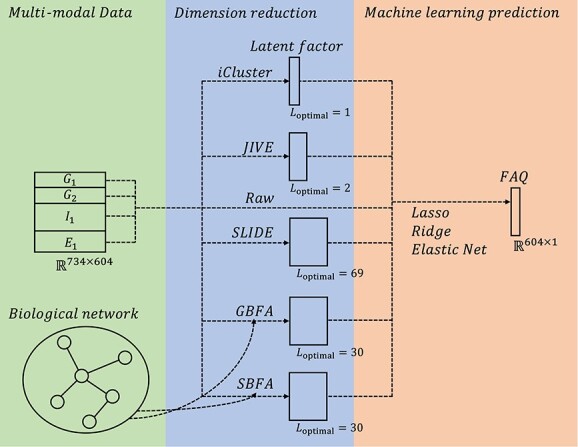
Workflow for real data analysis.  and
and  are genotyping data encoded by the presence of homozygous major allele and the presence of homozygous alternative allele, respectively.
  and
and  are normalized QTs representing the gene expression and neuroimaging data. Starting from the multi-modal data, different factor analysis methods are used to extract the latent factors. The number of latent dimensions is tuned either through the implemented function from the package or using BIC. After obtaining the latent factor, we use the latent factor as the input predictor to predict the FAQ score. Linear regression with lasso, ridge and elastic net regularizations are used. The raw data (transpose of multi-omics data), covariates and raw data plus covariates are also used for comparison purpose.
Our framework starts from the dimention reduction of multi-omics data including indicator variables for homozygous dominant genotyping data  , indicator variables for homozygous recessive genotyping data
  , AV45 imaging measurements
  and gene expression
  . Specifically,
  and
and  are binary matrices with dimension
  , the entries of which are assumed to follow the Bernoulli distribution.
  and
and  are normalized QTs with dimension
  and
and  , which are assumed to be normally distributed.
We estimate the latent factors from the multi-omics and imaging dataset using our proposed SBFA method, in comparison with several existing methods including iCluster+ [19, 71], JIVE [25], SLIDE [26] and GBFA [47]. For the hyperparameters, we fix  and tune
  . The best tuning results are obtained by minimizing the BIC criteria, which is presented in Figure 2. The best-tuned
  is indicated by
  , which is the number of columns of the corresponding latent factors. For our proposed SBFA model, the best-tuned hyperparameter set is
  . We then apply linear regression with lasso, ridge and elastic net regularizations models to predict the FAQ score using the latent factors learned from the aforementioned methods as predictors. For comparison purposes, we also include three other approaches that use (i) the demographic covariates, (ii) the multi-omics and imaging data and (iii) the multi-omics and imaging data together with the demographic covariates as the input of machine learning models, respectively; see Table 3.
Table 3.
Real data performance. The averaged MSE between the predicted FAQ score and the true FAQ score is reported across 100 random splittings. All standard errors are rounded to 0 after preserving 3 digits. For comparison purposes, we also include three other approaches that use (A) the demographic covariates, (B) the multi-omics and imaging data and (C) the multi-omics and imaging data together with the demographic covariates as the input of machine learning models.
Feature Method Method |
Lasso | Ridge | ElasticNet | ||||||
|---|---|---|---|---|---|---|---|---|---|
| Train | Validation | Test | Train | Validation | Test | Train | Validation | Test | |
| Raw data and clinical variables | |||||||||
| Demographic covariates | 0.626 | 0.955 | 0.953 | 0.592 | 0.934 | 0.949 | 0.596 | 0.938 | 0.945 |
| Multi-omics and imaging | 0.626 | 0.958 | 0.959 | 0.334 | 0.883 | 0.921 | 0.516 | 0.864 | 0.940 |
| Multi-omics, imaging and covariates | 0.622 | 0.957 | 0.956 | 0.333 | 0.886 | 0.933 | 0.517 | 0.864 | 0.940 |
| Latent factors | |||||||||
| JIVE | 0.638 | 0.964 | 0.963 | 0.638 | 0.964 | 0.963 | 0.638 | 0.964 | 0.963 |
| SLIDE | 0.638 | 0.964 | 0.963 | 0.478 | 0.920 | 0.908 | 0.638 | 0.963 | 0.963 |
| iCluster+ | 0.638 | 0.964 | 0.963 | 0.637 | 0.974 | 0.961 | 0.638 | 0.964 | 0.963 |
| GBFA | 0.528 | 0.894 | 0.918 | 0.452 | 0.803 | 0.911 | 0.483 | 0.842 | 0.918 |
| SBFA (proposed) | 0.538 | 0.896 | 0.893 | 0.454 | 0.850 | 0.881 | 0.466 | 0.853 | 0.895 |
For our training process, we first evenly split the subjects into five folds where 4-folds are treated as the training-validation set and 1-fold is treated as the testing set. Next, we apply 4-fold cross-validation in our training-validation set to select the best tuning hyperparameters according to the mean squared error (MSE). The best tuning models are obtained from the validation set and applied to the testing set to get the testing performance. We repeat the splitting and tuning process 100 times by randomly splitting the data 100 times with 100 different random seeds. We summarized our real data analysis results in Table 3. The real data analysis performance is reported using the mean of the training, validation and testing MSE across 100 random splits. The standard errors for the training and testing MSE are rounded to zero after preserving three digits.
As shown in Table 3, compared with the results using original multi-omics and imaging data and clinical variables, our SBFA method does a better job in mitigating the overfitting problem. In particular, the three prediction models trained using estimated factors from our SBFA method outperform the models trained using the original multi-omics, imaging and demographic variables, in spite of the fact that our factor analysis used only multi-omics and imaging data, not demographic variables. Compared with other existing factor analysis methods, our SBFA method yields the best performance (smallest MSE) across all comparisons (i.e. linear regression model with lasso, ridge and elastic net regularizations).
Simulation Study
We compared the performance of our proposed SBFA framework with other factor analysis frameworks including JIVE [25], SLIDE [26] and GBFA model with spike and slab prior and Markov random field prior [47] in the simulation study.
Simulation design
We evaluated our proposed SBFA framework in two different simulation scenarios—low dimensional scenario and high dimensional scenario with the number of features  and
and  , respectively. We used the same number of samples in both simulation scenarios with
  . To simulate multi-omics data, we used the following model:
 |
(6) |
where  ,
,  ,
, and
and  . We choose the ground truth latent variable
  and the number of datasets
  .
.
We design our ground-truth loading matrix  as shown in Figure 3, where each row represents a pathway (
 ). The shaded areas are generated by continuous uniform distribution with
  and every non-zero element of the loading matrix
  has a probability of
  to flip its sign.
Figure 3.
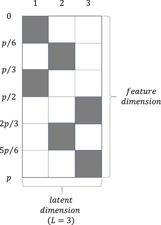
Groundtruth setting for factor loading matrix  . Numbers labeled on each column represent the latent variable. Numbers labeled on rows represent the number of rows from the first row to the corresponding row. All shaded area represents elements generated by
  with probability
  to be multiplied by
  . All the other area contains only zero elements.
The ground truth factor matrix  is simply generated by
 |
where  represents the zero vector, and
  represents the identity matrix.
The ground truth mean parameter for data  , i.e.
  , is obtained by
 |
where we assume location parameter  . For the first setting in each simulation scenario, we assume only Gaussian distribution with mean
  and standard deviation
  for all
  . For the second setting in each simulation scenario, we assume the first two omic datasets with
  features following Bernoulli distribution with each element having probability
  to be
to be  . It mimics the data structure for the allele homozygosity encoded genotyping dataset. For the second two omics datasets with
  features, we assume that they are generated by a binomial distribution with trail parameter independently sampled from the set
  . For each feature and each subject, we assume the success probability parameter
  . For the third two omics datasets with
  features, we assume that they are generated to mimic the gene expression and imaging data, which follows the Gaussian distribution with mean
  and standard deviation
  .
.
For the graph information, we evaluate our algorithm with  different settings:
Within-pathway edges only: For the first graph information setting, we randomly generate
 edges within each pathway and do not add across pathway edges (i.e. in total, we have
  within pathway edges for
  features). This is a simulation of an ideal case.
Within-pathway edges and cross pathway edges: For the second graph information setting, besides the
 within pathway edges generated in the first setting, we also randomly generate
  cross-pathway edges within each modality (i.e. in total, we have
  within pathway edges and
  cross-pathway edges for
  features).
The graph with within-pathway edges only represents the ideal case where the graphical structure coincides with the sparsity structure in  , while the cross-pathway edges mimic the real data.
Results
In our simulation study, we seek to reconstruct the mean matrix from the extracted low-rank representation. The performance is evaluated by the relative reconstruction error (RRE) between estimated  and true
  using Frobenius norm
 |
(7) |
where  denotes the ground truth mean parameter;
  represents the estimated mean parameter.
To reduce the randomness of the performance, we generate  different datasets and apply our proposed algorithm to obtain the new feature representation for each dataset. We fixed
  and tuned the
  parameters using BIC. We compare our SBFA framework with four different baseline factor analysis algorithms including JIVE, SLIDE, iCluster+ and GBFA.
We first evaluate our results by calculating the mean and the standard error of the RRE across  simulation datasets. It is worth noting that the best-tuned
  based on BIC is always equal to or larger than the ground truth. For those
  greater than the ground truth, compared with the other baseline methods, the estimated loadings by SBFA for the extra latent dimension(s) are exactly 0 except for a small number of nonzero entries (supplementary information Figure 1). The best-tuned results for each method and each simulation setting are summarized in Tables 4 and 5. Our proposed SBFA model always outperforms the other baseline methods in both the Gaussian distribution setting (Table 4) and the mixture distribution setting (Table 5).
Figure e1.

Estimated factor loadings for the simulated dataset. The heatmap shows the factor loadings from iCluster, JIVE, SLIDE and GBFA without graph information (GBFA(NE)), GBFA with graph information (GBFA(E)), SBFA without graph information (SBFA(NE)), SBFA with graph information (SBFA(E)) and the ground truth. The results are derived from one simulated dataset in the low-dimensional scenario ( ). The optimal latent dimension (
 ) for each model is indicated by the number of circles in the corresponding method track. Numbers beyond the range of (
 ) have the same color as the boundaries (
 and 1).
Table 4.
Simulation performance results for Gaussian only setting. ‘Dimension’ denotes our simulation scenario where ‘Low’ indicates the simulation scenario with  and ‘High’ indicates the simulation scenario with
  . ‘Edge’ represents different graph information where ‘Within’ denotes the ideal case that we use the graph information which only connects the features within each pathway, and ‘Cross’ denotes the case that we use the graph information that connects the features not only within each pathway but also some randomly selected nodes between pathways within each modality. ‘RRE (mean)’ is the average of the reconstruction error between estimated
  and the ground truth
  ratio to the true
  across 100 simulations. ‘RRE (se)’ is the standard error of the reconstruction error between estimated
  and the ground truth
  across 100 simulations.
| Method | Dimension | Edge | RRE (mean) | RRE (se) |
|---|---|---|---|---|
| JIVE | low | 0.236552 | 0.006583 | |
| SLIDE | low | 0.167271 | 0.000722 | |
| iCluster | low | 0.221568 | 0.000935 | |
GBFA ( ) ) |
low | Within | 0.198160 | 0.000848 |
GBFA ( ) ) |
low | Within | 0.190166 | 0.001088 |
SBFA (No  ) ) |
low | Within | 0.182882 | 0.000743 |
SBFA (With  ) ) |
low | Within | 0.180844 | 0.000699 |
GBFA ( ) ) |
low | Cross | 0.198160 | 0.000848 |
GBFA ( ) ) |
low | Cross | 0.185953 | 0.001015 |
SBFA (No  ) ) |
low | Cross | 0.182882 | 0.000743 |
SBFA (With  ) ) |
low | Cross | 0.181908 | 0.000704 |
| JIVE | high | 0.180514 | 0.001741 | |
| SLIDE | high | 0.154596 | 0.000727 | |
| iCluster | high | 0.188864 | 0.000806 | |
GBFA ( ) ) |
high | Within | 0.166760 | 0.000663 |
GBFA ( ) ) |
high | Within | 0.166246 | 0.000772 |
SBFA (No  ) ) |
high | Within | 0.153240 | 0.000686 |
SBFA (With  ) ) |
high | Within | 0.151277 | 0.000665 |
GBFA ( ) ) |
high | Cross | 0.166760 | 0.000663 |
GBFA ( ) ) |
high | Cross | 0.158246 | 0.000882 |
SBFA (No  ) ) |
high | Cross | 0.153240 | 0.000686 |
SBFA (With  ) ) |
high | Cross | 0.152455 | 0.000672 |
Table 5.
Simulation performance results for mixture distribution setting. ‘Dimension’ denotes our simulation scenario where ‘Low’ indicates the simulation scenario with  and ‘High’ indicates the simulation scenario with
  . ‘Edge’ represents different graph information where ‘Within’ denotes the ideal case that we use the graph information which only connects the features within each pathway, and ‘Cross’ denotes the case that we use the graph information that connects the features not only within each pathway but also some randomly selected nodes between pathways within each modality. ‘RRE (mean)’ is the average of the reconstruction error between estimated
  and the ground truth
  ratio to the true
  across 100 simulations. ‘RRE (se)’ is the standard error of the reconstruction error between estimated
  and the ground truth
  across 100 simulations.
| Method | Dataset | Edge | RRE (mean) | RRE (se) |
|---|---|---|---|---|
| JIVE | low | 1.539543 | 0.014274 | |
| SLIDE | low | 1.519234 | 0.010254 | |
| iCluster | low | 1.407917 | 0.011129 | |
GBFA ( ) ) |
low | Within | 0.220563 | 0.000961 |
GBFA ( ) ) |
low | Within | 0.220918 | 0.000993 |
SBFA (No  ) ) |
low | Within | 0.197850 | 0.000877 |
SBFA (With  ) ) |
low | Within | 0.196208 | 0.000864 |
GBFA ( ) ) |
low | Cross | 0.220563 | 0.000961 |
GBFA ( ) ) |
low | Cross | 0.217769 | 0.001006 |
SBFA (No  ) ) |
low | Cross | 0.197850 | 0.000877 |
SBFA (With  ) ) |
low | Cross | 0.199828 | 0.000874 |
| JIVE | high | 1.551844 | 0.007424 | |
| SLIDE | high | 1.508521 | 0.006791 | |
| iCluster | high | 1.397968 | 0.007480 | |
GBFA ( ) ) |
high | Within | 0.190666 | 0.000886 |
GBFA ( ) ) |
high | Within | 0.188583 | 0.000733 |
SBFA (No  ) ) |
high | Within | 0.175308 | 0.000773 |
SBFA (With  ) ) |
high | Within | 0.173823 | 0.000733 |
GBFA ( ) ) |
high | Cross | 0.190666 | 0.000886 |
GBFA ( ) ) |
high | Cross | 0.189722 | 0.000890 |
SBFA (No  ) ) |
high | Cross | 0.175308 | 0.000773 |
SBFA (With  ) ) |
high | Cross | 0.177781 | 0.000764 |
In the Gaussian distribution setting (Table 4), without incorporating the graph information, our proposed model (SBFA No  ) shows significant improvement compared with JIVE, SLIDE, iCluster+ and GBFA without graph information (GBFA
  ). By taking the graph information into consideration, our proposed model (SBFA With
  ) can further achieve a smaller RRE and significantly outperforms the GBFA model (GBFA
  ) both with and without cross pathway noise.
In the mixture distribution setting (Table 5), JIVE, SLIDE and iCluster yield a large RRE compared with GBFA and SBFA models. This is expected because those methods handle the discrete data by treating them as continuous random variables. Although the GBFA model and our proposed SBFA model can both handle discrete and continuous data simultaneously, our SBFA model outperforms the GBFA model in both low-dimensional simulation and high-dimensional simulation scenarios with or without incorporating the graph information.
In summary, our proposed SBFA model can handle discrete and continuous data simultaneously. Our simulation study demonstrates that our proposed SBFA model can outperform the most state-of-the-art factor analysis models. Moreover, our SBFA model can incorporate the biological graph information as prior knowledge so that our model can produce biologically interpretable results.
Conclusion
In this article, we proposed a structural Bayesian factor analysis model which decomposes the underlying mean parameters of the data into a sparse factor loading matrix and factor matrix. Our model employed the Laplace prior to achieve the sparse estimation of the loading matrix and used a graph Laplacian prior to incorporate the biological network information. Our method can handle both discrete and continuous data simultaneously. We derived an efficient variational EM algorithm to obtain the MAP estimators of the parameters of interest.
Our SBFA framework is a useful dimension reduction technique that yields latent factors that are biologically interpretable. As such, the common information shared among multi-modal data learned from our model can be used for various downstream machine learning tasks including, but not limited to, prediction. For example, another potential application is to use learned factors for clustering which can be used to define disease subtypes based on genotyping data, imaging modalities and biological pathways.
Our simulation study demonstrates that our proposed SBFA framework achieves the best performance compared with the other state-of-the-art factor-analysis-based integrative methods. Our work bridges the gap that there are few multi-omics studies applied to AD. We used the multi-omics data from the ADNI dataset to predict the FAQ score, which is an important evaluation for the diagnosis of AD. The real data analysis results show the advantages of our framework by comparing the prediction performance between our SBFA framework and other state-of-the-art factor-analysis-based integrative methods. Our method exhibited the best prediction performance.
Key Points
We propose a novel structural Bayesian factor analysis framework as a dimension reduction technique that yields latent factors by integrating the genotyping data, gene expression data, region-level brain imaging amyloid deposition data and biological network information. Our SBFA framework is biologically interpretable. The common information shared among multi-omics data learned from our model can be used for various subsequent analyses such as supervised and unsupervised machine learning.
Our structural Bayesian factor analysis model can handle both continuous (e.g. gene expression and imaging phenotypic traits) and discrete [e.g. genotyping values for single nucleotide polymorphisms (SNPs)] datatypes simultaneously.
Our work bridges the gap that there are few multi-omics studies applied to Alzheimer’s disease. We applied our framework to extract biologically meaningful information shared by multiple modalities in the ADNI database. We performed the subsequent machine learning analyses to predict the Alzheimer’s disease-related cognitive score using the extracted latent factors. Our structural Bayesian factor analysis model achieves the best prediction accuracy for the subsequent machine learning prediction problems compared with the other state-of-the-art factor-analysis-based methods.
Acknowledgements
This study was partly supported by NIH grants RF1AG063481, R01AG071174, R01 AG071470, U01 AG066833 and U01 AG068057. Data used in this study were obtained from the ADNI database (adni.loni.usc.edu), which was funded by NIH U01AG024904.
Jingxuan Bao is a Ph.D. student co-advised by Dr. Li Shen and Dr. Qi Long at the University of Pennsylvania Perelman School of Medicine.
Changgee Chang is an assistant professor at Indiana University School of Medicine.
Qiyiwen Zhang is a postdoctoral fellow in Dr. Qi Long’s lab at the University of Pennsylvania Perelman School of Medicine.
Andrew J. Saykin is the director of the Center for Neuroimaging and Indiana Alzheimer's Disease Research Center. He is a professor at Indiana University School of Medicine.
Li Shen is a Professor of Informatics at the University of Pennsylvania Perelman School of Medicine.
Qi Long is a Professor of Biostatistics at the University of Pennsylvania.
Data used in preparation of this article were obtained from the Alzheimer's Disease Neuroimaging Initiative (ADNI) database (adni.loni.ucla.edu). As such, the investigators within the ADNI contributed to the design and implementation of ADNI and/or provided data but did not participate in analysis or writing of this report. A complete listing of ADNI investigators can be found at: {http://adni.loni.usc.edu/wp-content/uploads/how_to_apply/ADNI_Acknowledgement_List.pdf}.
Contributor Information
Jingxuan Bao, Department of Biostatistics, Epidemiology and Informatics, University of Pennsylvania Perelman School of Medicine, Philadelphia, 19104, PA, USA.
Changgee Chang, Department of Biostatistics, Epidemiology and Informatics, University of Pennsylvania Perelman School of Medicine, Philadelphia, 19104, PA, USA.
Qiyiwen Zhang, Department of Biostatistics, Epidemiology and Informatics, University of Pennsylvania Perelman School of Medicine, Philadelphia, 19104, PA, USA.
Andrew J Saykin, Department of Radiology and Imaging Sciences, Indiana University, Indianapolis, 46202, IN, USA.
Li Shen, Department of Biostatistics, Epidemiology and Informatics, University of Pennsylvania Perelman School of Medicine, Philadelphia, 19104, PA, USA.
Qi Long, Department of Biostatistics, Epidemiology and Informatics, University of Pennsylvania Perelman School of Medicine, Philadelphia, 19104, PA, USA.
Data availability
The source code is available through GitHub (https://github.com/JingxuanBao/SBFA). The genotyping data, gene expression data, demographic data, and imaging data used in the preparation of this article were obtained from the Alzheimer's Disease Neuroimaging Initiative (ADNI) database. The data are available after application through the ADNI website (http://adni.loni.usc.edu).
Author contributions statement
Jingxuan Bao and Dr. Changgee Chang take full responsibility for the integrity of the data and the accuracy of the data analysis.
Study concept and design: Jingxuan Bao, Dr. Changgee Chang and Dr. Qi Long.
Acquisition, analysis or interpretation of data: Jingxuan Bao, Dr. Changgee Chang, Dr. Andrew J. Saykin, Dr. Li Shen and Dr. Qi Long.
Drafting of the manuscript: Jingxuan Bao, Dr. Changgee Chang and Dr. Qi Long.
Critical revision of the manuscript for important intellectual content: All authors.
Study supervision: Dr. Changgee Chang and Dr. Qi Long.
References
- 1. Subramanian I, Verma S, Kumar S, et al. Multi-omics data integration, interpretation, and its application. Bioinform Biol Insights 2020; 14:1177932219899051. [DOI] [PMC free article] [PubMed] [Google Scholar]
- 2. Trambaiolli LR, Lorena AC, Fraga FJ, et al. Improving alzheimer’s disease diagnosis with machine learning techniques. Clin EEG Neurosci 2011; 42(3): 160–5. [DOI] [PubMed] [Google Scholar]
- 3. Kim M, Bao J, Liu K, et al. Structural connectivity enriched functional brain network using simplex regression with graphnet. In: Machine Learning in Medical Imaging. Cham: Springer International Publishing, 2020, 292–302. [DOI] [PMC free article] [PubMed] [Google Scholar]
- 4. Kim M, Bao J, Liu K, et al. A structural enriched functional network: an application to predict brain cognitive performance. Med Image Anal 2021; 71:102026. [DOI] [PMC free article] [PubMed] [Google Scholar]
- 5. Kochunov P, Zavaliangos-Petropulu A, Jahanshad N, et al. A white matter connection of schizophrenia and Alzheimer’s disease. Schizophr Bull 2020; 47(1): 197–206. [DOI] [PMC free article] [PubMed] [Google Scholar]
- 6. Sendi MSE, Zendehrouh E, Miller RL, et al. Alzheimer’s disease projection from normal to mild dementia reflected in functional network connectivity: a longitudinal study. Front Neural Circuits 2021; 14: 593263. [DOI] [PMC free article] [PubMed] [Google Scholar]
- 7. Sendi MSE, Zendehrouh E, Fu Z, et al. Disrupted dynamic functional network connectivity among cognitive control networks in the progression of alzheimer’s disease. Brain Connect 2021. [DOI] [PMC free article] [PubMed] [Google Scholar]
- 8. Wan J, Zhang Z, Rao BD, et al. Identifying the neuroanatomical basis of cognitive impairment in alzheimer’s disease by correlation- and nonlinearity-aware sparse bayesian learning. IEEE Trans Med Imaging 2014; 33(7): 1475–87. [DOI] [PMC free article] [PubMed] [Google Scholar]
- 9. Madar IH, Sultan G, Tayubi IA, et al. Identification of marker genes in alzheimer’s disease using a machine-learning model. Bioinformation 2021; 17(2): 348–55. [DOI] [PMC free article] [PubMed] [Google Scholar]
- 10. Ferreira D, Nordberg A, Westman E. Biological subtypes of alzheimer disease. Neurology 2020; 94(10): 436–48. [DOI] [PMC free article] [PubMed] [Google Scholar]
- 11. Jellinger KA. Pathobiological subtypes of alzheimer disease. Dement Geriatr Cogn Disord 2021; 49:321–33. [DOI] [PubMed] [Google Scholar]
- 12. Lin D, Cao H, Calhoun VD, et al. Sparse models for correlative and integrative analysis of imaging and genetic data. J Neurosci Methods 2014; 237:69–78. [DOI] [PMC free article] [PubMed] [Google Scholar]
- 13. Zhu X, Yao J, Xiao G, et al. Imaging-genetic data mapping for clinical outcome prediction via supervised conditional gaussian graphical model. In: 2016 IEEE International Conference on Bioinformatics and Biomedicine (BIBM). New York City, USA: Institute of electrical and electronics engineers (IEEE), pp. 455–9, 2016.
- 14. Batmanghelich NK, Dalca A, Quon G, et al. Probabilistic modeling of imaging, genetics and diagnosis. IEEE Trans Med Imaging 2016; 35(7): 1765–79. [DOI] [PMC free article] [PubMed] [Google Scholar]
- 15. Shen L, Thompson PM. Brain imaging genomics: integrated analysis and machine learning. Proc IEEE 2020; 108(1): 125–62. [DOI] [PMC free article] [PubMed] [Google Scholar]
- 16. Shen L, Kim S, Qi Y, et al. Identifying neuroimaging and proteomic biomarkers for mci and ad via the elastic net. Multimodal Brain Image Analysis 2011; 7012:27–34. [DOI] [PMC free article] [PubMed] [Google Scholar]
- 17. Wang H, Nie F, Huang H, et al. Identifying disease sensitive and quantitative trait-relevant biomarkers from multidimensional heterogeneous imaging genetics data via sparse multimodal multitask learning. Bioinformatics 2012; 28(12): i127–36. [DOI] [PMC free article] [PubMed] [Google Scholar]
- 18. Wang D, Gu J. Integrative clustering methods of multi-omics data for molecule-based cancer classifications. Quant Biol 2016; 4(1): 58–67. [Google Scholar]
- 19. Shen R, Olshen AB, Ladanyi M. Integrative clustering of multiple genomic data types using a joint latent variable model with application to breast and lung cancer subtype analysis. Bioinformatics 2009; 25(22): 2906–12. [DOI] [PMC free article] [PubMed] [Google Scholar]
- 20. Shen R, Wang S, Mo Q. Sparse integrative clustering of multiple omics data sets. Ann Appl Stat 2013; 7(1): 269–94. [DOI] [PMC free article] [PubMed] [Google Scholar]
- 21. Chauvel C, Novoloaca A, Veyre P, et al. Evaluation of integrative clustering methods for the analysis of multi-omics data. Brief Bioinform 2019; 21(2): 541–52. [DOI] [PubMed] [Google Scholar]
- 22. Chalise P, Fridley BL. Integrative clustering of multi-level ‘omic data based on non-negative matrix factorization algorithm. PLoS One 2017; 12(5): 1–18. [DOI] [PMC free article] [PubMed] [Google Scholar]
- 23. Ahmed KT, Sun J, Cheng S, et al. Multi-omics data integration by generative adversarial network. Bioinformatics 2021; 38(1): 179–86. [DOI] [PMC free article] [PubMed] [Google Scholar]
- 24. Mo Q, Wang S, Seshan VE, et al. Pattern discovery and cancer gene identification in integrated cancer genomic data. Proc Natl Acad Sci U S A 2013; 110(11): 4245–50. [DOI] [PMC free article] [PubMed] [Google Scholar]
- 25. Lock EF, Hoadley KA, Marron JS, et al. Joint and individual variation explained (JIVE) for integrated analysis of multiple data types. Ann Appl Stat 2013; 7(1): 523–42. [DOI] [PMC free article] [PubMed] [Google Scholar]
- 26. Gaynanova I, Li G. Structural learning and integrative decomposition of multi-view data. Biometrics 2019; 75(4): 1121–32. [DOI] [PubMed] [Google Scholar]
- 27. Murray ME, Graff-Radford NR, Ross OA, et al. Neuropathologically defined subtypes of alzheimer’s disease with distinct clinical characteristics: a retrospective study. Lancet Neurol 2011; 10(9): 785–96. [DOI] [PMC free article] [PubMed] [Google Scholar]
- 28. Whitwell JL, Dickson DW, Murray ME, et al. Neuroimaging correlates of pathologically defined subtypes of alzheimer’s disease: a case-control study. Lancet Neurol 2012; 11(10): 868–77. [DOI] [PMC free article] [PubMed] [Google Scholar]
- 29. Neff RA, Wang M, Vatansever S, et al. Molecular subtyping of alzheimer’s disease using rna sequencing data reveals novel mechanisms and targets. Sci Adv 2021; 7(2): eabb5398. [DOI] [PMC free article] [PubMed] [Google Scholar]
- 30. Di Fede G, Catania M, Maderna E, et al. Molecular subtypes of alzheimer’s disease. Sci Rep 2018; 8(1): 3269. [DOI] [PMC free article] [PubMed] [Google Scholar]
- 31. Levin F, Ferreira D, Lange C, et al. Data-driven fdg-pet subtypes of alzheimer’s disease-related neurodegeneration. Alzheimer’s Res Ther 2021; 13(1): 49. [DOI] [PMC free article] [PubMed] [Google Scholar]
-
32.
Qiang W, Yau WM, Jun-Xia L, et al. Structural variation in amyloid-
 fibrils from alzheimer’s disease clinical subtypes. Nature 2017; 541(7636): 217–21. [DOI] [PMC free article] [PubMed] [Google Scholar]
 - 33. Wong AK, Krishnan A, Yao V, et al. IMP 2.0: a multi-species functional genomics portal for integration, visualization and prediction of protein functions and networks. Nucleic Acids Res 2015; 43(W1): W128–33. [DOI] [PMC free article] [PubMed] [Google Scholar]
- 34. Kanehisa M, Goto S. KEGG: Kyoto Encyclopedia of genes and genomes. Nucleic Acids Res 2000; 28(1): 27–30. [DOI] [PMC free article] [PubMed] [Google Scholar]
- 35. Kanehisa M. Toward understanding the origin and evolution of cellular organisms. Protein Sci 2019; 28(11): 1947–51. [DOI] [PMC free article] [PubMed] [Google Scholar]
- 36. Kanehisa M, Furumichi M, Sato Y, et al. KEGG: integrating viruses and cellular organisms. Nucleic Acids Res 2020; 49(D1): D545–51. [DOI] [PMC free article] [PubMed] [Google Scholar]
- 37. Zhou J, Troyanskaya OG. Predicting effects of noncoding variants with deep learning–based sequence model. Nat Methods 2015; 12(10): 931–4. [DOI] [PMC free article] [PubMed] [Google Scholar]
- 38. Zhou J, Theesfeld CL, Yao K, et al. Deep learning sequence-based ab initio prediction of variant effects on expression and disease risk. Nat Genet 2018; 50(8): 1171–9. [DOI] [PMC free article] [PubMed] [Google Scholar]
- 39. Krishnan A, Zhang R, Yao V, et al. Genome-wide prediction and functional characterization of the genetic basis of autism spectrum disorder. Nat Neurosci 2016; 19(11): 1454–62. [DOI] [PMC free article] [PubMed] [Google Scholar]
- 40. Greene CS, Krishnan A, Wong AK, et al. Understanding multicellular function and disease with human tissue-specific networks. Nat Genet 2015; 47(6): 569–76. [DOI] [PMC free article] [PubMed] [Google Scholar]
- 41. Li C, Li H. Network-constrained regularization and variable selection for analysis of genomic data. Bioinformatics 2008; 24(9): 1175–82. [DOI] [PubMed] [Google Scholar]
- 42. Pan W, Xie B, Shen X. Incorporating predictor network in penalized regression with application to microarray data. Biometrics 2010; 66(2): 474–84. [DOI] [PMC free article] [PubMed] [Google Scholar]
- 43. Li F, Zhang NR. Bayesian variable selection in structured high-dimensional covariate spaces with applications in genomics. J Am Stat Assoc 2010; 105(491): 1202–14. [Google Scholar]
- 44. Stingo FC, Chen YA, Tadesse MG, et al. Incorporating biological information into linear models: a bayesian approach to the selection of pathways and genes. Ann Appl Stat 2011; 5(3): 1978–2002. [DOI] [PMC free article] [PubMed] [Google Scholar]
- 45. Chang C, Kundu S, Long Q. Scalable bayesian variable selection for structured high-dimensional data. Biometrics 2018; 74(4): 1372–82. [DOI] [PMC free article] [PubMed] [Google Scholar]
- 46. Rockova V, Lesaffre E. Incorporating grouping information in Bayesian variable selection with applications in genomics. Bayesian Anal 2014; 9(1): 221–58. [Google Scholar]
- 47. Min EJ, Chang C, Long Qi. Generalized bayesian factor analysis for integrative clustering with applications to multi-omics data. In: 2018 IEEE 5th International Conference on Data Science and Advanced Analytics (DSAA). New York City, USA: Institute of electrical and electronics engineers (IEEE), pp. 109–19, 2018. [DOI] [PMC free article] [PubMed]
- 48. Coniglio A, Nappi CR, Peruggi F, et al. Percolation and phase transitions in the ising model. Commun Math Phys 1976; 51(3): 315–23. [Google Scholar]
- 49. Dubes RC, Jain AK, Nadabar SG, Chen CC. Mrf model-based algorithms for image segmentation. In: [1990] Proceedings. 10th International Conference on Pattern Recognition. New York City, USA: Institute of electrical and electronics engineers (IEEE), pp. 808–14, vol. 1, 1990. [Google Scholar]
- 50. Chung FR. Spectral graph theory. Rhode Island, US: American Mathematical Soc, 1997. [Google Scholar]
- 51. Ng AY, Jordan MI, Weiss Y. On spectral clustering: Analysis and an algorithm. In: Proceedings of the 14th International Conference on Neural Information Processing Systems: Natural and Synthetic, NIPS’01. Cambridge, Massachusetts, USA: Massachusetts Institute of Technology (MIT), pp. 849–56. MIT Press, 2001. [Google Scholar]
- 52. Polson NG, Scott JG, Windle J. Bayesian inference for logistic models using pólya–gamma latent variables. J Am Stat Assoc 2013; 108(504): 1339–49. [Google Scholar]
- 53. Dempster AP, Laird NM, Rubin DB. Maximum likelihood from incomplete data via the em algorithm. J R Stat Soc B Methodol 1977; 39(1): 1–38. [Google Scholar]
- 54. Girolami M. A Variational method for learning sparse and overcomplete representations. Neural Comput 2001; 13(11, 11): 2517–32. [DOI] [PubMed] [Google Scholar]
- 55. Blei DM, Kucukelbir A, McAuliffe JD. Variational inference: a review for statisticians. J Am Stat Assoc 2017; 112(518): 859–77. [Google Scholar]
- 56. Corless RM, Gonnet GH, Hare DEG, et al. On the lambertw function. Adv Comput Math 1996; 5(1): 329–59. [Google Scholar]
- 57. Mezo I, Baricz A. On the generalization of the lambert w function. Trans Am Math Soc 2017; 7(369): 7917–34. [Google Scholar]
- 58. Chang C, Tsay RS. Estimation of covariance matrix via the sparse cholesky factor with lasso. J Stat Plan Inference 2010; 140(12): 3858–73. [Google Scholar]
- 59. Saykin AJ, Shen L, Yao X, et al. Genetic studies of quantitative MCI and AD phenotypes in ADNI: progress, opportunities, and plans. Alzheimers Dement 2015; 11(7): 792–814. [DOI] [PMC free article] [PubMed] [Google Scholar]
- 60. Shen L, Thompson PM, Potkin SG, et al. Genetic analysis of quantitative phenotypes in AD and MCI: imaging, cognition and biomarkers. Brain Imaging Behav 2014; 8(2): 183–207. [DOI] [PMC free article] [PubMed] [Google Scholar]
- 61. Weiner MW, Veitch DP, Aisen PS, et al. Recent publications from the Alzheimer’s Disease Neuroimaging Initiative: reviewing progress toward improved AD clinical trials. Alzheimers Dement 2017; 13(4): e1–85. [DOI] [PMC free article] [PubMed] [Google Scholar]
- 62. Pfeffer RI, Kurosaki TT, Harrah CH, Jr, et al. Measurement of functional activities in older adults in the community. J Gerontol 1982; 37(3): 323–9. [DOI] [PubMed] [Google Scholar]
- 63. Seshadri S, Fitzpatrick AL, Ikram MA, et al. Genome-wide analysis of genetic loci associated with Alzheimer disease. JAMA 2010; 303(18): 1832–40. [DOI] [PMC free article] [PubMed] [Google Scholar]
- 64. Lambert JC, Ibrahim-Verbaas CA, Harold D, et al. Meta-analysis of 74,046 individuals identifies 11 new susceptibility loci for Alzheimer’s disease. Nat Genet 2013; 45(12): 1452–8. [DOI] [PMC free article] [PubMed] [Google Scholar]
- 65. Jansen IE, Savage JE, Watanabe K, et al. Genome-wide meta-analysis identifies new loci and functional pathways influencing Alzheimer’s disease risk. Nat Genet 2019; 51(3): 404–13. [DOI] [PMC free article] [PubMed] [Google Scholar]
-
66.
Kunkle B, Benjamin G-B, Rebecca S, et al. Genetic meta-analysis of diagnosed Alzheimer’s disease identifies new risk loci and implicates A
 , tau, immune and lipid processing. Nat Genet 2019; 51:414–30. [DOI] [PMC free article] [PubMed] [Google Scholar]
 - 67. Bellenguez C, Kucukali F, Jansen I, et al. New insights into the genetic etiology of Alzheimer’s disease and related dementias. Nat Genet 2020; 54: 412–36. [DOI] [PMC free article] [PubMed] [Google Scholar]
- 68. Chang CC, Chow CC, Tellier LCAM, et al. Second-generation plink: rising to the challenge of larger and richer datasets. GigaScience 2015; 4:7. [DOI] [PMC free article] [PubMed] [Google Scholar]
- 69. Piñero J, Ramírez-Anguita JM, Saüch-Pitarch J, et al. The DisGeNET knowledge platform for disease genomics: 2019 update. Nucleic Acids Res 2019; 48(D1): D845–55. [DOI] [PMC free article] [PubMed] [Google Scholar]
- 70. Glasser MF, Coalson TS, Robinson EC, et al. A multi-modal parcellation of human cerebral cortex. Nature 2016; 536(7615): 171–8. [DOI] [PMC free article] [PubMed] [Google Scholar]
- 71. Mo Q, Shen R. iClusterPlus: integrative clustering of multi-type genomic data. R package version 2021; 1.28.0. http://52.71.54.154/packages/release/bioc/html/iClusterPlus.html. [Google Scholar]
Associated Data
This section collects any data citations, data availability statements, or supplementary materials included in this article.
Data Availability Statement
The source code is available through GitHub (https://github.com/JingxuanBao/SBFA). The genotyping data, gene expression data, demographic data, and imaging data used in the preparation of this article were obtained from the Alzheimer's Disease Neuroimaging Initiative (ADNI) database. The data are available after application through the ADNI website (http://adni.loni.usc.edu).