Two optimized novel potential formulas and numerical algorithms for $m\times n$ cobweb and fan resistor networks

Abstract

The research of resistive network will become the basis of many fields. At present, many exact potential formulas of some complex resistor networks have been obtained. Computer numerical simulation is the trend of computing, but written calculation will limit the time and scale. In this paper, the potential formulas of a $m\times n$ scale cobweb resistor network and fan resistor network are optimized. Chebyshev polynomial of the second class and the absolute value function are used to express the novel potential formulas of the resistor network, and described in detail the derivation process of the explicit formula. Considering the influence of parameters on the potential formulas, several idiosyncratic potential formulas are proposed, and the corresponding three-dimensional dynamic images are drawn. Two numerical algorithms of the computing potential are presented by using the mathematical model and DST-VI. Finally, the efficiency of calculating potential by different methods are compared. The advantages of new potential formulas and numerical algorithms by the calculation efficiency of the three methods are shown. The optimized potential formulas and the presented numerical algorithms provide a powerful tool for the field of science and engineering.

Introduction

Tan¹ creatively established the mathematical model of cobweb and fan resistor networks, according to this model, gave the incomparable analytical potential formula in theory. This is a breakthrough work, and its theoretical significance and application prospects are huge. As is well-known, classical physics is based on the analysis of physics mathematical models of physical processes. Computers have given physicists and engineers a new way to analyze and apply physical formulas and mathematical models that has revolutionized science and engineering outside the university. Everything changes if the computer is used to analyze and apply physical formulas and mathematical models. In addition, experts in engineering and scientific computing know that to improve the computational efficiency of the potential to help computational physicists and engineers solve major scientific and technical problems, it is a good idea to optimize the perfect analytical potential formula given in theory to improve the computational efficiency. In order to improve the calculation performance and scale of the formula. In this paper, based on the original potential formula, we re-represent it with the Chebyshev polynomial of the second class and the absolute value function, which improves the computational efficiency, and design the numerical algorithms can be used to the calculating potential for large-scale resistor networks.

In the process of scientific development, many complex problems have arisen, which often require simple models to solve. According to the research results of resistor network model^2–11 and neural network model^12–18, ideas can be obtained on many complex problems. In the past many years, through the research results of Green’s function, Laplace equation, Poisson equation, finite and infinite dimensional resistor network and Laplace matrix (LM) method and so on^{8–11,19–32}, the foundation of resistor network research has been laid. Shi et al.^12,13 studied a new discrete time recurrent neural network and its application to manipulators. Sun et al.^14,15 studied the theory and application of noise tolerance zeroing neural network. And Jin et al.^16–18 proposed a modified Zhang neural network (MZNN) model for the solution of time-varying quadratic programing (TVQP).

In the past few years, Tan et al.^33–53 proposed a simpler recursive transformation (RT) method than LM method in the research of resistance network. It simplified the Laplacian matrix in two directions to the Laplacian matrix in one direction. In 2014, Tan et al.³⁷ solved the potential formula of spherical resistance network for the first time. Since 2015, Tan et al.^34–44 has studied the resistance network model by RT method. After 2020, Tan et al.^45–53 made more in-depth research on resistance network. Since RT method requires using a tridiagonal matrix to construct a mathematical model, and the analytical potential formula must be expressed by using the exact eigenvalues of this tridiagonal matrix. So the exact eigenvalues of the tridiagonal matrix need to be found. Tridiagonal matrices are used in many areas of science and engineering, and there are many good conclusions about it^54–61.

In 2017, Tan¹ used RT-V method for the first time to study cobweb network and fan network. In Figs. 1 and 2, the resistance on the warp and weft lines is $r_0$ and r, where m and n are the scale of the resistor network, it contains m rows and n columns. Point $O_{(0,0)}=0$ is defined as the origin of the resistor network. The potential formula $U_{m\times n}(x,y)$ of any node d(x, y) in the $m\times n$ cobweb network is shown as

$$\begin{array}{c}\hfill \frac{U_{m\times n}(x,y)}{J}=\frac{4r}{2m+1}\sum _{i=1}^m\frac{g_{x_1,x}^{(i)}{S}_{y_1,i}-g_{x_2,x}^{(i)}{S}_{y_2,i}}{{\lambda }_i^n+{\overline{\lambda }}_i^n-2}{S}_{y,i},\end{array}$$ 1

$$\begin{array}{c}\hfill g_{x_s,x}^{(i)}=F_{n-|x_s-x|}+F_{|x_s-x|}.\end{array}$$ 2

The potential formula $U_{m\times n}(x,y)$ of any node d(x, y) in the $m\times n$ fan network is shown as

$$\begin{array}{c}\hfill \frac{U_{m\times n}(x,y)}{J}=\frac{4r}{2m+1}\sum _{i=1}^m\frac{{\beta }_{x_1,x}^{(i)}{S}_{y_1,i}-{\beta }_{x_2,x}^{(i)}{S}_{y_2,i}}{(t_i-2)F_{n+1}^{(i)}}{S}_{y,i},\end{array}$$ 3

$$\begin{array}{c}\hfill {\beta }_{x_s,x}^{(i)}=\left\{\begin{array}{c}\hfill \mathrm{\Delta }{F}_{x_s}^{(i)}\mathrm{\Delta }{F}_{n-x}^{(i)}ifx\ge x_s,\\ \hfill \mathrm{\Delta }{F}_x^{(i)}\mathrm{\Delta }{F}_{n-x_s}^{(i)}ifx\le x_s,\end{array}\right)\end{array}$$ 4

where ${\theta }_i=\frac{(2i-1)\pi }{(2m+1)},S_{y_k,i}=sin(y_k{\theta }_i)$

$$\begin{array}{c}\hfill F_k^{(i)}=\frac{{\lambda }_i^k-{\overline{\lambda }}_i^k}{{\lambda }_i-{\overline{\lambda }}_i},\end{array}$$ 5

$$\begin{array}{cc}\hfill & {\lambda }_i=1+h-hcos{\theta }_i+\sqrt{{(1+h-hcos{\theta }_i)}^2-1},\hfill \\ \hfill & {\overline{\lambda }}_i=1+h-hcos{\theta }_i-\sqrt{{(1+h-hcos{\theta }_i)}^2-1},\hfill \end{array}$$ 6

$$\begin{array}{c}\hfill t_i=2+2h-2hcos{\theta }_i,\end{array}$$ 7

the parameter $h=\frac{r}{r_0}$ is defined.

Figure 1.

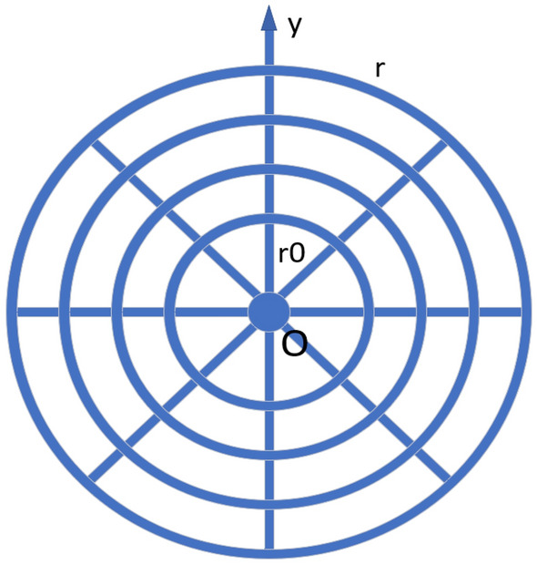
A $8\times 4$ cowbeb resistor network containing $8\times 4$ nodes and a zero potential point O.

Figure 2.

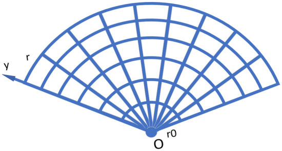
A $10\times 6$ fan resistor network containing $10\times 6$ nodes and a zero potential point O.

Novel formulas of potential represented by Chebyshev polynomials

This section presents the re-expressed potential formulas (1) and (3)¹ of the resistor network. The potential formula expressed by the Chebyshev polynomial of the second class⁶² can reduce the running time of computer simulation.

Assume that the current J is input from $d_1(x_1,y_1)$ and output from $d_2(x_2,y_2)$. The potential formula of any node d(x, y) in the $m\times n$ cobweb resistor network is

$$\begin{array}{c}\hfill \frac{{\mathbf{U}}_{m\times n}(x,y)}{J}=\frac{4r}{2m+1}\sum _{\iota =1}^m\frac{{\mu }_{x_1,x}^{(\iota )}{S}_{y_1,\iota }-{\mu }_{x_2,x}^{(\iota )}{S}_{y_2,\iota }}{U_n^{(\iota )}-U_{n-2}^{(\iota )}-2}{S}_{y,\iota },\end{array}$$ 8

where

$$\begin{array}{c}\hfill {\mu }_{x_s,x}^{(\iota )}=U_{n-|x_s-x|-1}^{(\iota )}+U_{|x_s-x|-1}^{(\iota )},s=1,2.\end{array}$$ 9

The potential formula of any node d(x, y) in the $m\times n$ fan resistor network is

$$\begin{array}{c}\hfill \frac{{\mathcal{U}}_{m\times n}(x,y)}{J}=\frac{4r}{2m+1}\sum _{\iota =1}^m\frac{{\epsilon }_{x_1,x}^{(\iota )}{S}_{y_1,\iota }-{\epsilon }_{x_2,x}^{(\iota )}{S}_{y_2,\iota }}{({\omega }_{\iota }-2)U_n^{(\iota )}}{S}_{y,\iota },\end{array}$$ 10

where

$$\begin{array}{c}\hfill {\epsilon }_{x_s,x}^{(\iota )}={(U_{-0.5}^{(\iota )})}^2(U_{n-|x_s-x|+1}^{(\iota )}-U_{n-|x_s-x|-1}^{(\iota )}+U_{n-x_s-x}^{(\iota )}-U_{n-x_s-x-2}^{(\iota )}),s=1,2,\end{array}$$ 11

$$\begin{array}{c}\hfill S_{y_k,\iota }=sin(\frac{y_k(2\iota -1)\pi }{2m+1}),k=1,2,\end{array}$$ 12

$$\begin{array}{c}\hfill {\omega }_{\iota }=2+\frac{2r}{r_0}-\frac{2r}{r_0}cos\frac{(2\iota -1)\pi }{2m+1},\end{array}$$ 13

$$\begin{array}{c}\hfill U_{\nu }^{(\iota )}=U_{\nu }^{(\iota )}(cosh{\varphi }_{\iota })=\frac{sinh(\nu +1){\varphi }_{\iota }}{sinh({\varphi }_{\iota })},cosh{\varphi }_{\iota }=\frac{{\omega }_{\iota }}{2},\frac{{\omega }_{\iota }}{2}>1,{\varphi }_{\iota }>0,\end{array}$$ 14

$$\begin{array}{c}\hfill v=n-|x_s-x|-1,|x_s-x|-1,n-2,n-|x_s-x|+1,n-x_s-x,n-x_s-x-2,n,-0.5,s=1,2,\iota =1,2,\dots ,m.\end{array}$$

We set the node voltage at point $O_{(0,0)}$ to 0, and the formula for calculating the potential of any node is described as

$$\begin{array}{c}\hfill {\mathbf{U}}_{m\times n}(x,y)={\mathbf{V}}_x^{(y)},{\mathcal{U}}_{m\times n}(x,y)={\mathcal{V}}_x^{(y)},V_0^{(0)}=0,\end{array}$$ 15

where ${\mathbf{V}}_x^{(y)}$ and ${\mathcal{V}}_x^{(y)}$ are denoted by the node voltage of any node.

Horadam sequence and discrete sine transform

In this section, we introduce the explicit formula of Horadam sequence which is expressed by the Chebyshev polynomial of the second class and the sixth kind of discrete sine transform.

A second-order recurrence sequence $W_v$ is called a Horadam sequence if

$$\begin{array}{c}\hfill W_v=d{W}_{v-1}-q{W}_{v-2},W_0=a,W_1=b,\end{array}$$ 16

where $v\in \mathbf{N},v\ge 2,a,b,d,q\in \mathbb{C}$, $\mathbf{N}$ is set of all nonnegative integers and $\mathbb{C}$ is the set of all complex numbers.

The explicit formula of Horadam sequence expressed by the Chebyshev polynomial of the second class is⁶³

$$\begin{array}{c}\hfill W_v={(\sqrt{q})}^v\left(\frac{b}{\sqrt{q}},U_{v-1},\left(\frac{d}{2\sqrt{q}}\right),-,a,U_{v-2},\left(\frac{d}{2\sqrt{q}}\right)\right),\end{array}$$ 17

where $U_v$ is the Chebyshev polynomial of the second class⁶², i.e.

$$\begin{array}{c}\hfill U_v=U_v(cos\varphi )=\frac{sin(v+1)\varphi }{sin\varphi },cos\varphi =\frac{d}{2\sqrt{q}},\varphi \in \mathbb{C}.\end{array}$$ 18

If $\frac{d}{2\sqrt{q}}>1$, the Chebyshev polynomial of the second class is re-described by hyperbolic functions, then Eq. (18) is transformed into

$$\begin{array}{c}\hfill U_v=U_v(cosh\varphi )=\frac{sinh(v+1)\varphi }{sinh\varphi },cosh\varphi =\frac{d}{2\sqrt{q}},\varphi \in \mathbb{R},\end{array}$$ 19

where $\mathbb{R}$ is the set of all real numbers.

First, we will present the derivation of Eq. (5) represented by the Chebyshev polynomial of the second class.

Remark 1

It can be obtained from Eq. (6) that ${\lambda }_{\iota }+{\overline{\lambda }}_{\iota }={\omega }_{\iota }$ and ${\lambda }_{\iota }·{\overline{\lambda }}_{\iota }=1$. Adding these conditions to Eq. (16), we get the following special Horadam sequence

$$\begin{array}{c}\hfill F_v^{(\iota )}={\omega }_{\iota }{F}_{v-1}^{(\iota )}-F_{v-2}^{(\iota )},F_0^{(\iota )}=0,F_1^{(\iota )}=1,\end{array}$$ 20

where $d={\omega }_{\iota }>2,q=1$, $F_v^{(\iota )}$ and ${\omega }_{\iota }$ are expressed in Eqs. (5) and (13), respectively. By replacing the expression of Eq. (5), with the results of Eq. (19), we have

$$\begin{array}{c}\hfill F_v^{(\iota )}=\frac{{\lambda }_{\iota }^v-{\overline{\lambda }}_{\iota }^v}{{\lambda }_{\iota }-{\overline{\lambda }}_{\iota }}=U_{v-1}^{(\iota )}(\frac{{\omega }_{\iota }}{2}).\end{array}$$ 21

Secondly, we will give the derivation of ${\lambda }_{\iota }^n+{\overline{\lambda }}_{\iota }^n$ expressed by the Chebyshev polynomial of the second class.

Remark 2

Let

$$\begin{array}{c}\hfill B_n^{(\iota )}={\lambda }_{\iota }^n+{\overline{\lambda }}_{\iota }^n,\end{array}$$ 22

where $B_0^{(\iota )}=2,B_1^{(\iota )}={\omega }_{\iota }$.

Then the recursive relation of $B_n^{(\iota )}$ is expressed as

$$\begin{array}{c}\hfill B_n^{(\iota )}={\omega }_{\iota }{B}_{n-1}^{(\iota )}-B_{n-2}^{(\iota )},B_0^{(\iota )}=2,B_1^{(\iota )}={\omega }_{\iota },\end{array}$$ 23

where $d={\omega }_{\iota },q=1$, ${\omega }_{\iota }$ and $B_n^{(\iota )}$ are expressed in Eqs. (13) and (22), respectively.

By Eqs. (17) and (19), $B_n^{(\iota )}$ is represented as follows

$$\begin{array}{c}\hfill B_n^{(\iota )}={\lambda }_{\iota }^n+{\overline{\lambda }}_{\iota }^n={\omega }_{\iota }{U}_{n-1}(\frac{{\omega }_{\iota }}{2})-2U_{n-2}(\frac{{\omega }_{\iota }}{2})=U_n(\frac{{\omega }_{\iota }}{2})-U_{n-2}(\frac{{\omega }_{\iota }}{2}).\end{array}$$ 24

Next, we will show the derivation of replacing Eq. (4) in terms of piecewise functions with Eq. (11) in terms of absolute value functions.

Remark 3

For Eq. (4), when $x\ge x_s$

$$\begin{array}{c}\hfill \begin{array}{cc}\hfill {\beta }_{x_s,x}^{(\iota )}=& (F_{x_s+1}^{(\iota )}-F_{x_s}^{(\iota )})(F_{n-x+1}^{(\iota )}-F_{n-x}^{(\iota )})\hfill \\ \hfill =& \left(\frac{{\lambda }_{\iota }^{n-x+x_s+2}+{\overline{\lambda }}_{\iota }^{n-x+x_s+2}-{\lambda }_{\iota }^{n-x+x_s+1}-{\overline{\lambda }}_{\iota }^{n-x+x_s+1}}{{({\lambda }_{\iota }-{\overline{\lambda }}_{\iota })}^2},-,\frac{{\lambda }_{\iota }^{n-x+x_s+1}+{\overline{\lambda }}_{\iota }^{n-x+x_s+1}-{\lambda }_{\iota }^{n-x+x_s}-{\overline{\lambda }}_{\iota }^{n-x+x_s}}{{({\lambda }_{\iota }-{\overline{\lambda }}_{\iota })}^2}\right)\hfill \\ \hfill & +\left(\frac{{\lambda }_{\iota }^{n-x-x_s+1}+{\overline{\lambda }}_{\iota }^{n-x-x_s+1}-{\lambda }_{\iota }^{n-x-x_s}-{\overline{\lambda }}_{\iota }^{n-x-x_s}}{{({\lambda }_{\iota }-{\overline{\lambda }}_{\iota })}^2},-,\frac{{\lambda }_{\iota }^{n-x-x_s}+{\overline{\lambda }}_{\iota }^{n-x-x_s}-{\lambda }_{\iota }^{n-x-x_s-1}-{\overline{\lambda }}_{\iota }^{n-x-x_s-1}}{{({\lambda }_{\iota }-{\overline{\lambda }}_{\iota })}^2}\right)\hfill \\ \hfill =& \left(\frac{({\lambda }_{\iota }-1){\lambda }_{\iota }^{n-x+x_s+1}+({\overline{\lambda }}_{\iota }-1){\overline{\lambda }}_{\iota }^{n-x+x_s+1}-(1-{\overline{\lambda }}_{\iota }){\lambda }_{\iota }^{n-x+x_s+1}-(1-{\lambda }_{\iota }){\overline{\lambda }}_{\iota }^{n-x+x_s+1}}{{({\lambda }_{\iota }-{\overline{\lambda }}_{\iota })}^2}\right)\hfill \\ \hfill & +\left(\frac{({\lambda }_{\iota }-1){\lambda }_{\iota }^{n-x-x_s}+({\overline{\lambda }}_{\iota }-1){\overline{\lambda }}_{\iota }^{n-x-x_s}-(1-{\overline{\lambda }}_{\iota }){\lambda }_{\iota }^{n-x-x_s}-(1-{\lambda }_{\iota }){\overline{\lambda }}_{\iota }^{n-x-x_s}}{{({\lambda }_{\iota }-{\overline{\lambda }}_{\iota })}^2}\right)\hfill \\ \hfill =& \frac{({\lambda }_{\iota }+{\overline{\lambda }}_{\iota }-2)({\lambda }_{\iota }^{n-x+x_s+1}+{\overline{\lambda }}_{\iota }^{n-x+x_s+1}+{\lambda }_{\iota }^{n-x-x_s}+{\overline{\lambda }}_{\iota }^{n-x-x_s})}{{({\lambda }_{\iota }-{\overline{\lambda }}_{\iota })}^2}\hfill \\ \hfill =& \frac{{({\lambda }_{\iota }^{0.5}-{\overline{\lambda }}_{\iota }^{0.5})}^2}{{({\lambda }_{\iota }-{\overline{\lambda }}_{\iota })}^2}\left({\lambda }_{\iota }^{n-x+x_s+1},+,{\overline{\lambda }}_{\iota }^{n-x+x_s+1},+,{\lambda }_{\iota }^{n-x-x_s},+,{\overline{\lambda }}_{\iota }^{n-x-x_s}\right)\hfill \\ \hfill =& {(F_{0.5}^{(\iota )})}^2(F_{n-(x-x_s)+2}^{(\iota )}-F_{n-(x-x_s)}^{(\iota )}+F_{n-x-x_s+1}^{(\iota )}-F_{n-x-x_s-1}^{(\iota )}).\hfill \end{array}\end{array}$$ 25

Similarly, when $x\le x_s$

$$\begin{array}{c}\hfill \begin{array}{cc}\hfill {\beta }_{x_s,x}^{(\iota )}=& (F_{x+1}^{(\iota )}-F_x^{(\iota )})(F_{n-x_s+1}^{(\iota )}-F_{n-x_s}^{(\iota )})\hfill \\ \hfill =& \left(\frac{{\lambda }_{\iota }^{n-x_s+x+2}+{\overline{\lambda }}_{\iota }^{n-x_s+x+2}-{\lambda }_{\iota }^{n-x_s+x+1}-{\overline{\lambda }}_{\iota }^{n-x_s+x+1}}{{({\lambda }_{\iota }-{\overline{\lambda }}_{\iota })}^2},-,\frac{{\lambda }_{\iota }^{n-x_s+x+1}+{\overline{\lambda }}_{\iota }^{n-x_s+x+1}-{\lambda }_{\iota }^{n-x_s+x}-{\overline{\lambda }}_{\iota }^{n-x_s+x}}{{({\lambda }_{\iota }-{\overline{\lambda }}_{\iota })}^2}\right)\hfill \\ \hfill & +\left(\frac{{\lambda }_{\iota }^{n-x_s-x+1}+{\overline{\lambda }}_{\iota }^{n-x_s-x+1}-{\lambda }_{\iota }^{n-x_s-x}-{\overline{\lambda }}_{\iota }^{n-x_s-x}}{{({\lambda }_{\iota }-{\overline{\lambda }}_{\iota })}^2},-,\frac{{\lambda }_{\iota }^{n-x_s-x}+{\overline{\lambda }}_{\iota }^{n-x_s-x}-{\lambda }_{\iota }^{n-x_s-x-1}-{\overline{\lambda }}_{\iota }^{n-x_s-x-1}}{{({\lambda }_{\iota }-{\overline{\lambda }}_{\iota })}^2}\right)\hfill \\ \hfill =& \left(\frac{({\lambda }_{\iota }-1){\lambda }_{\iota }^{n-x_s+x+1}+({\overline{\lambda }}_{\iota }-1){\overline{\lambda }}_{\iota }^{n-x_s+x+1}-(1-{\overline{\lambda }}_{\iota }){\lambda }_{\iota }^{n-x_s+x+1}-(1-{\lambda }_{\iota }){\overline{\lambda }}_{\iota }^{n-x_s+x+1}}{{({\lambda }_{\iota }-{\overline{\lambda }}_{\iota })}^2}\right)\hfill \\ \hfill & +\left(\frac{({\lambda }_{\iota }-1){\lambda }_{\iota }^{n-x_s-x}+({\overline{\lambda }}_{\iota }-1){\overline{\lambda }}_{\iota }^{n-x_s-x}-(1-{\overline{\lambda }}_{\iota }){\lambda }_{\iota }^{n-x_s-x}-(1-{\lambda }_{\iota }){\overline{\lambda }}_{\iota }^{n-x_s-x}}{{({\lambda }_{\iota }-{\overline{\lambda }}_{\iota })}^2}\right)\hfill \\ \hfill =& \frac{({\lambda }_{\iota }+{\overline{\lambda }}_{\iota }-2)({\lambda }_{\iota }^{n-x_s+x+1}+{\overline{\lambda }}_{\iota }^{n-x_s+x+1}+{\lambda }_{\iota }^{n-x_s-x}+{\overline{\lambda }}_{\iota }^{n-x_s-x})}{{({\lambda }_{\iota }-{\overline{\lambda }}_{\iota })}^2}\hfill \\ \hfill =& \frac{{({\lambda }_{\iota }^{0.5}-{\overline{\lambda }}_{\iota }^{0.5})}^2}{{({\lambda }_{\iota }-{\overline{\lambda }}_{\iota })}^2}({\lambda }_{\iota }^{n-x_s+x+1}+{\overline{\lambda }}_{\iota }^{n-x_s+x+1}+{\lambda }_{\iota }^{n-x_s-x}+{\overline{\lambda }}_{\iota }^{n-x_s-x})\hfill \\ \hfill =& {(F_{0.5}^{(\iota )})}^2(F_{n-(x_s-x)+2}^{(\iota )}-F_{n-(x_s-x)}^{(\iota )}+F_{n-x_s-x+1}^{(\iota )}-F_{n-x_s-x-1}^{(\iota )}).\hfill \end{array}\end{array}$$ 26

Combining Eqs. (25) and (26), Eq. (4) is re-expressed by the absolute value functions as

$$\begin{array}{c}\hfill {\beta }_{x_s,x}^{(i)}={(F_{0.5}^{(\iota )})}^2(F_{n-|x_s-x|+2}^{(\iota )}-F_{n-|x_s-x|}^{(\iota )}+F_{n-x_s-x+1}^{(\iota )}-F_{n-x_s-x-1}^{(\iota )}),s=1,2,\end{array}$$ 27

By Eqs. (21), (27) and (11) in terms of the Chebyshev polynomial of the second class and absolute value function is obtained.

Using Eqs. (19), (21) and (24), the potential formulas (8) and (10) are obtained.

In order to achieve the fast calculation of numerical simulation, we utilize the sixth kind of discrete sine transform to diagonalize the perturbed tridiagonal matrix ${\mathbf{A}}_m$¹.

$$\begin{array}{c}\hfill {\mathbf{A}}_m={\left(\begin{array}{ccccc}2+2h& -h& 0& \cdots & 0\\ -h& 2+2h& -h& \ddots & ⋮\\ 0& \ddots & \ddots & \ddots & 0\\ ⋮& \ddots & -h& 2+2h& -h\\ 0& \cdots & 0& -h& 2+h\end{array}\right)}_{m\times m},\end{array}$$ 28

where $h=\frac{r}{r_0}$.

The eigenvectors ${\omega }_1,\dots ,{\omega }_m$ of matrix ${\mathbf{A}}_m$ are expressed as

$$\begin{array}{c}\hfill {\omega }_{\iota }=2+2h-2hcos\frac{(2\iota -1)\pi }{2m+1}),\iota =1,2,\dots ,m,\end{array}$$ 29

and the corresponding eigenvectors ${\alpha }^{(j)}={({\alpha }_1^{(j)},{\alpha }_2^{(j)},\dots ,{\alpha }_m^{(j)})}^T$ are expressed as

$$\begin{array}{c}\hfill {\alpha }_k^{(j)}=\frac{2}{\sqrt{2m+1}}sin\frac{(2j-1)k\pi }{2m+1},k=1,2,\dots ,m,j=1,2,\dots ,m.\end{array}$$ 30

As is known to all, if the orthogonal matrix ${\mathbb{S}}_m^{\mathit{VI}}$ is the sixth kind of discrete sine transform (DST-VI)^64–68, where

$$\begin{array}{c}\hfill {\mathbb{S}}_m^{\mathit{VI}}=\frac{2}{\sqrt{2m+1}}{\left(sin,\frac{(2j-1)k\pi }{2m+1}\right)}_{k,j=1}^m,\end{array}$$ 31

then

$$\begin{array}{c}\hfill {({\mathbb{S}}_m^{\mathit{VI}})}^{-1}={({\mathbb{S}}_m^{\mathit{VI}})}^T={\mathbb{S}}_m^{\mathit{VII}},\end{array}$$ 32

where ${({\mathbb{S}}_m^{\mathit{VI}})}^T$ is the transpose of the matrix ${\mathbb{S}}_m^{\mathit{VI}}$ and ${\mathbb{S}}_m^{\mathit{VII}}$ is the seventh kind of discrete sine transform (DST-VII).

The process of realizing the orthogonal diagonalization of matrix ${\mathbf{A}}_m$ by ${\mathbb{S}}_m^{\mathit{VI}}$ is as follows

$$\begin{array}{c}\hfill {({\mathbb{S}}_m^{\mathit{VI}})}^{-1}{\mathbf{A}}_m({\mathbb{S}}_m^{\mathit{VI}})=\text{diag}({\omega }_1,{\omega }_2,\dots ,{\omega }_m),\end{array}$$ 33

i.e.,

$$\begin{array}{c}\hfill {\mathbf{A}}_m=({\mathbb{S}}_m^{\mathit{VI}})\text{diag}({\omega }_1,{\omega }_2,\dots ,{\omega }_m){({\mathbb{S}}_m^{\mathit{VI}})}^{-1},\end{array}$$ 34

where ${\omega }_{\iota }$ is given by Eq. (29).

By Kirchhoff’ s law and the node voltage, Tan¹ gave a matrix equation model as follows

$$\begin{array}{c}\hfill {\mathbf{V}}_{v+1}={\mathbf{A}}_m{\mathbf{V}}_v-{\mathbf{V}}_{v-1}-r{\mathbf{I}}_v,\end{array}$$ 35

where ${\mathbf{A}}_m$ in Eq. (28), ${\mathbf{V}}_v$ and ${\mathbf{I}}_v$ are vectors of length $m\times 1$, in which ${\delta }_{k,v}(v=k)=1$, ${\delta }_{k,v}(v\ne k)=0$.

$$\begin{array}{c}\hfill {\mathbf{V}}_v={[V_v^{(1)},V_v^{(2)},...V_v^{(m)}]}^T(0\le v\le n),\end{array}$$ 36

$$\begin{array}{c}\hfill I_v^{(\iota )}=J({\delta }_{x_1,v}-{\delta }_{x_2,v}).\end{array}$$ 37

Since Eq. (35) cannot be directly calculated. Equation (35) is transformed by ${\mathbb{S}}_m^{\mathit{VI}}$ method. The process of transformation is as follows.

$$\begin{array}{c}\hfill {({\mathbb{S}}_m^{\mathit{VI}})}^{-1}{\mathbf{V}}_v={({\mathbb{S}}_m^{\mathit{VI}})}^T{\mathbf{V}}_v={\mathbf{C}}_v,{\mathbf{V}}_v={\mathbb{S}}_m^{\mathit{VI}}{\mathbf{C}}_v,\end{array}$$ 38

where ${\mathbf{C}}_v$ is also a $m\times 1$ vector

$$\begin{array}{c}\hfill {\mathbf{C}}_v={[c_v^{(1)},c_v^{(2)},...,c_v^{(m)}]}^T(0\le v\le n).\end{array}$$ 39

Remark 4

Tan¹ proposed the node voltage formula of the cobweb network as follows

$$\begin{array}{c}\hfill V_k^{(y)}=J\frac{4r}{2m+1}\sum _{i=1}^m\frac{g_{x_1,x}^{(i)}{S}_{y_1,i}-g_{x_2,x}^{(i)}{S}_{y_2,i}}{{\lambda }_i^n+{\overline{\lambda }}_i^n-2}sin(y{\theta }_i),\end{array}$$ 40

where $g_{x_1,x}^{(i)}$ is expressed in Eq. (2), ${\lambda }_i^n$ and ${\overline{\lambda }}_i^n$ is in Eq. (6), ${\theta }_i=\frac{(2i-1)\pi }{(2m+1)}$, $S_{y_k,i}=sin(y_k{\theta }_i),k=1,2$.

According to Eqs. (2), (21), (24) and (40), we re-express the node voltage formula by the Chebyshev polynomial of the second class as follows

$$\begin{array}{c}\hfill {\mathbf{V}}_v^{(y)}=J\frac{4r}{2m+1}\sum _{\iota =1}^m\frac{{\mu }_{x_1,x}^{(\iota )}{S}_{y_1,\iota }-{\mu }_{x_2,x}^{(\iota )}{S}_{y_2,\iota }}{U_n^{(\iota )}-U_{n-2}^{(\iota )}-2}{S}_{y,\iota },\end{array}$$ 41

where ${\mu }_{x_s,x}^{(\iota )},s=1,2$ is same as Eq. (9), $U_v^{(\iota )}$ is same as Eq. (14), and $S_{y_s,\iota }$ is same as Eq. (12).

According to Eqs. (38), (39) and (41), we can get the analytic formula of ${\mathbf{c}}_x^{(\iota )}$ as

$$\begin{array}{c}\hfill {\mathbf{c}}_x^{(\iota )}=\frac{2rJ}{\sqrt{2m+1}}\left(\frac{{\mu }_{x_1,x}^{(\iota )}{S}_{y_1,\iota }-{\mu }_{x_2,x}^{(\iota )}{S}_{y_2,\iota }}{U_n^{(\iota )}-U_{n-2}^{(\iota )}-2}\right),(0\le x\le n),\end{array}$$ 42

Tan¹ proposed the node voltage formula of the fan network as follows

$$\begin{array}{c}\hfill V_k^{(y)}=J\frac{4r}{2m+1}\sum _{i=1}^m\frac{{\beta }_{x_1,x}^{(i)}{S}_{y_1,i}-{\beta }_{x_2,x}^{(i)}{S}_{y_2,i}}{(t_i-2)F_{n+1}^{(i)}}sin(y{\theta }_i),\end{array}$$ 43

where ${\beta }_{x_s,x}^{(i)}$ is expressed in Eq. (4), $F_k^{(i)}$ is given in Eq. (5), $t_i$ is given in Eq.  (7), ${\theta }_i=\frac{(2i-1)\pi }{(2m+1)}$, $S_{y_k,i}=sin(y_k{\theta }_i),k=1,2$.

According to Eqs. (4), (7), (13), (21) and (43), we re-express the node voltage formula by the Chebyshev polynomial of the second class as follows

$$\begin{array}{c}\hfill {\mathcal{V}}_v^{(y)}=J\frac{4r}{2m+1}\sum _{\iota =1}^m\frac{{\epsilon }_{x_1,x}^{(\iota )}{S}_{y_1,\iota }-{\epsilon }_{x_2,x}^{(\iota )}{S}_{y_2,\iota }}{({\omega }_{\iota }-2)U_n^{(\iota )}}{S}_{y,\iota },\end{array}$$ 44

where ${\epsilon }_{x_s,x}^{(\iota )},s=1,2$ is same as Eq.  (11), $S_{y_s,\iota }$ is same as Eq. (12), ${\omega }_{\iota }$ is same as Eq. (13) and $U_v^{(\iota )}$ is same as Eq. (14).

According to Eqs. (38), (39) and (44), we can get the analytic formula of $c_x^{(\iota )}$ as

$$\begin{array}{c}\hfill c_x^{(\iota )}=\frac{2rJ}{\sqrt{2m+1}}\left(\frac{{\epsilon }_{x_1,x}^{(\iota )}{S}_{y_1,\iota }-{\epsilon }_{x_2,x}^{(\iota )}{S}_{y_2,\iota }}{({\omega }_{\iota }-2)U_n^{(\iota )}}\right),(0\le x\le n),\end{array}$$ 45

Displaying of some special and interesting potential formulae

According to the obtained resistor network potential formulas (8) and (10) which contain multiple variables, this chapter analyzed the influence of different variables on the resistance network potential formula from two directions, assigned corresponding variables according to the conditions, and drew a three-dimensional dynamic view intuitive display.

Idiosyncratic potential formulas with the change of current input point and output point position

This section discusses the influence of changes in the position of the input and output points of the current in the resistor network on the potentials, as reflected in the three-dimensional dynamic view.

Idiosyncratic potential formula 1. If the current J flows in point $d_1(x_1,y_1)$ and out of $d_2(x_2,y_2)=O_{(0,0)}$, then a novel potential formula of the cobweb resistor network can be rewritten as

$$\begin{array}{c}\hfill \frac{{\mathbf{U}}_{m\times n}(x,y)}{J}=\frac{4r}{2m+1}\sum _{\iota =1}^m\frac{{\mu }_{x_1,x}^{(\iota )}{S}_{y_1,\iota }}{U_n^{(\iota )}-U_{n-2}^{(\iota )}-2}{S}_{y,\iota },\end{array}$$ 46

and a novel potential formula of the fan resistor network can be rewritten as

$$\begin{array}{c}\hfill \frac{{\mathcal{U}}_{m\times n}(x,y)}{J}=\frac{4r}{2m+1}\sum _{\iota =1}^m\frac{{\epsilon }_{x_1,x}^{(\iota )}{S}_{y_1,\iota }-{\epsilon }_{x_2,x}^{(\iota )}{S}_{y_2,\iota }}{({\omega }_{\iota }-2)U_n^{(\iota )}}{S}_{y,\iota },\end{array}$$ 47

where ${\mu }_{x_s,x}^{(\iota )},s=1,2$ is defined in Eq.  (9), ${\epsilon }_{x_s,x}^{(\iota )},s=1,2,$ is defined in Eq. (11), $U_v^{(\iota )}$ is defined in Eq. (14), and $S_{y_s,\iota }$ is defined in Eq. (12).

Let $m=n=60,J=10,x_1=y_1=20,x_2=y_2=0$, and $r_0=r=1$ in Eqs. (46) and (47), respectively. Then a special potential formula of the cobweb resistor network is obtained as follows

$$\begin{array}{c}\hfill \frac{{\mathbf{U}}_{60\times 60}(x,y)}{J}=\frac{4}{121}\sum _{\iota =1}^{60}\frac{{\mu }_{20,x}^{(\iota )}{S}_{20,\iota }}{U_{60}^{(\iota )}-U_{58}^{(\iota )}-2}{S}_{y,\iota },\end{array}$$ 48

and a special potential formula of the fan resistor network is obtained as follows

$$\begin{array}{c}\hfill \frac{{\mathcal{U}}_{60\times 60}(x,y)}{J}=\frac{4}{121}\sum _{\iota =1}^{60}\frac{{\epsilon }_{20,x}^{(\iota )}{S}_{20,\iota }}{({\omega }_{\iota }-2)U_{60}^{(\iota )}}{S}_{y,\iota },\end{array}$$ 49

where

$$\begin{array}{c}\hfill {\mu }_{20,x}^{(\iota )}=U_{59-|20-x|}^{(\iota )}+U_{|20-x|-1}^{(\iota )},\end{array}$$ 50

$$\begin{array}{c}\hfill {\epsilon }_{20,x}^{(\iota )}={(U_{-0.5}^{(\iota )})}^2(U_{61-|20-x|}^{(\iota )}-U_{59-|20-x|}^{(\iota )}+U_{40-x}^{(\iota )}-U_{38-x}^{(\iota )}),\end{array}$$ 51

$$\begin{array}{c}\hfill {\omega }_{\iota }=4-2cos\frac{(2\iota -1)\pi }{121},\end{array}$$ 52

$$\begin{array}{c}\hfill S_{20,\iota }=sin(\frac{(40\iota -20)\pi }{121}),\end{array}$$ 53

$$\begin{array}{c}\hfill U_{\nu }^{(\iota )}=U_{\nu }^{(\iota )}(cosh{\varphi }_{\iota })=\frac{sinh(\nu +1){\varphi }_{\iota }}{sinh({\varphi }_{\iota })},cosh{\varphi }_{\iota }=\frac{{\omega }_{\iota }}{2},\end{array}$$ 54

$$\begin{array}{c}\hfill S_{y,\iota }=sin\left(\frac{y(2\iota -1)\pi }{121}\right),\end{array}$$ 55

$$\begin{array}{c}\hfill v=61-|20-x|,59-|20-x|,|20-x|-1,40-x,38-x,60,58,-0.5.\iota =1,2,\dots ,60.\end{array}$$

And the three-dimensional dynamic views for the generative process of the potential graph are shown in Figs. 3 and 4, respectively.

Figure 3.

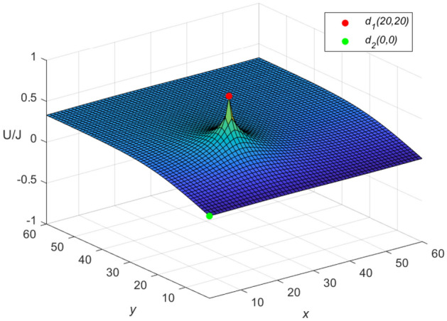
The potential graph for ${\mathbf{U}}_{60\times 60}(x,y)/J$ with the cobweb resistor network in Eq. (48).

Figure 4.

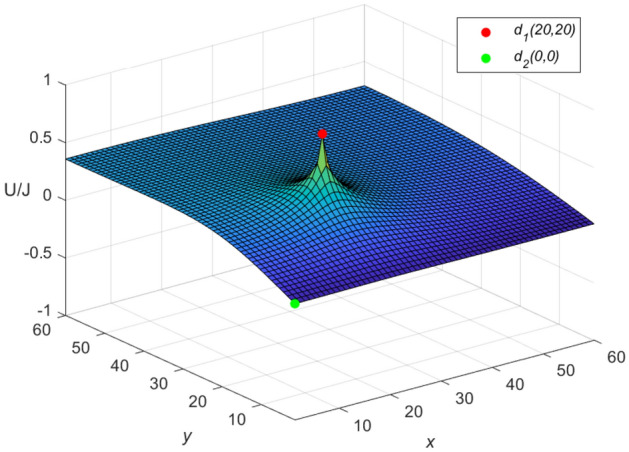
The potential graph for ${\mathcal{U}}_{60\times 60}(x,y)/J$ with the fan resistor network in Eq. (49).

Idiosyncratic potential formula 2. If the current J flows in from point $d_1(x_1,y_1)$ and out of $d_2(x_2,y_1)$, then a novel potential formula of the cobweb resistor network can be rewritten as

$$\begin{array}{c}\hfill \frac{{\mathbf{U}}_{m\times n}(x,y)}{J}=\frac{4r}{2m+1}\sum _{\iota =1}^m\frac{({\mu }_{x_1,x}^{(\iota )}-{\mu }_{x_2,x}^{(\iota )})S_{y_1,\iota }}{U_n^{(\iota )}-U_{n-2}^{(\iota )}-2}{S}_{y,\iota },\end{array}$$ 56

and a novel potential formula of the fan resistor network can be rewritten as

$$\begin{array}{c}\hfill \frac{{\mathcal{U}}_{m\times n}(x,y)}{J}=\frac{4r}{2m+1}\sum _{\iota =1}^m\frac{({\epsilon }_{x_1,x}^{(\iota )}-{\epsilon }_{x_2,x}^{(\iota )})S_{y_1,\iota }}{({\omega }_{\iota }-2)U_n^{(\iota )}}{S}_{y,\iota },\end{array}$$ 57

where ${\mu }_{x_s,x}^{(\iota )}$, ${\epsilon }_{x_s,x}^{(\iota )}$, $S_{y_s,\iota }$ and $U_v^{(\iota )}$ are same as Eqs. (9), (11), (12) and (14), respectively.

Let $m=n=60$, $J=10$, $y_1=y_2=x_1=20$, $x_2=40$, and $r_0=r=1$ in Eqs. (56) and (57), respectively. Then an idiosyncratic potential formula of the cobweb resistor network is given by

$$\begin{array}{c}\hfill \frac{{\mathbf{U}}_{m\times n}(x,y)}{J}=\frac{4}{121}\sum _{\iota =1}^{60}\frac{({\mu }_{20,x}^{(\iota )}-{\mu }_{40,x}^{(\iota )})S_{20,\iota }}{U_{60}^{(\iota )}-U_{58}^{(\iota )}-2}{S}_{y,\iota },\end{array}$$ 58

$$\begin{array}{c}\hfill {\mu }_{40,x}^{(\iota )}=U_{59-|40-x|}^{(\iota )}+U_{|40-x|-1}^{(\iota )},\end{array}$$ 59

and an idiosyncratic potential formula of the fan resistor network is given by

$$\begin{array}{c}\hfill \frac{{\mathcal{U}}_{m\times n}(x,y)}{J}=\frac{4}{121}\sum _{\iota =1}^{60}\frac{({\epsilon }_{20,x}^{(\iota )}-{\epsilon }_{40,x}^{(\iota )})S_{20,\iota }}{({\omega }_{\iota }-2)U_{60}^{(\iota )}}{S}_{y,\iota },\end{array}$$ 60

$$\begin{array}{c}\hfill {\epsilon }_{40,x}^{(\iota )}={(U_{-0.5}^{(\iota )})}^2(U_{61-|40-x|}^{(\iota )}-U_{59-|40-x|}^{(\iota )}+U_{20-x}^{(\iota )}-U_{18-x}^{(\iota )}),\end{array}$$ 61

where ${\mu }_{20,x}^{(\iota )}$, ${\epsilon }_{20,x}^{(\iota )}$, ${\omega }_{\iota }$, $S_{20,\iota }$ and $S_{y,\iota }$ are expressed in Eqs. (50), (51), (52), (53) and (55), respectively, with $v=61-|20-x|,61-|40-x|,59-|20-x|,59-|40-x|,|20-x|-1,|40-x|-1,40-x,38-x,20-x,18-x,60,58,-0.5,\iota =1,2,\dots ,60$.

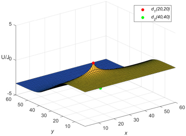
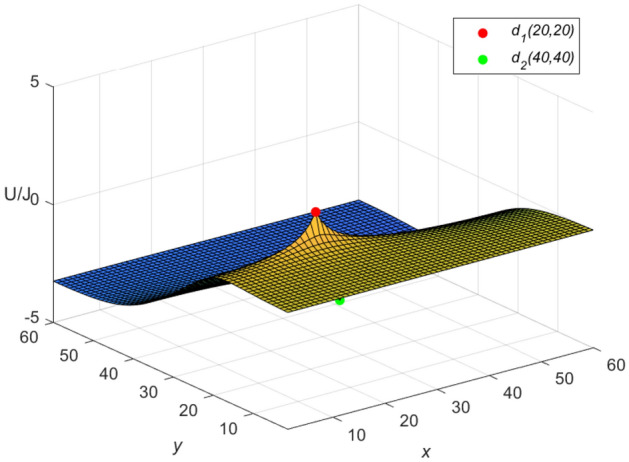
And the three-dimensional dynamic views for the generative process of the potential graph are shown in Figs. 5 and 6 by Matlab.

Figure 5.

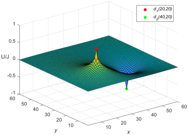
The potential graph for ${\mathbf{U}}_{60\times 60}(x,y)/J$ with the cobweb resistor network in Eq. (58).

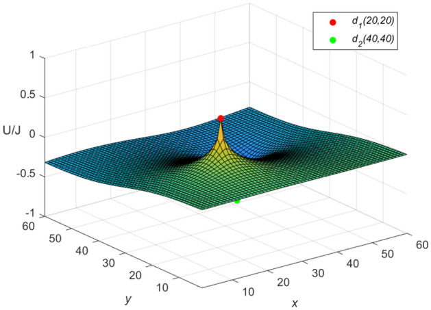
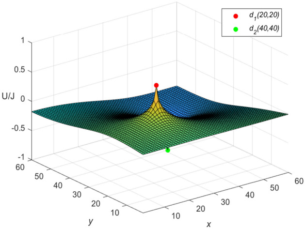
Figure 6.

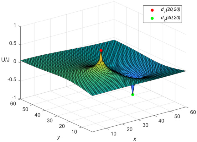
The potential graph for ${\mathcal{U}}_{60\times 60}(x,y)/J$ with the fan resistor network in Eq. (60).

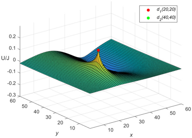
Idiosyncratic potential formula 3. If the current J/h flows in from point $d_s(x_s,y_1)(s=1,2,\dots ,h)$ and the current J out of $d_2(x_2,y_1)$, then a novel potential formula of the cobweb resistor network can be rewritten as

$$\begin{array}{c}\hfill \frac{{\mathbf{U}}_{m\times n}(x,y)}{J}=\frac{4r}{2m+1}\sum _{\iota =1}^m\frac{{\sum }_{s=1}^h{\mu }_{x_s,x}^{(\iota )}{S}_{y_1,\iota }-{\mu }_{x_2,x}^{(\iota )}{S}_{y_2,\iota }}{U_n^{(\iota )}-U_{n-2}^{(\iota )}-2}{S}_{y,\iota },\end{array}$$ 62

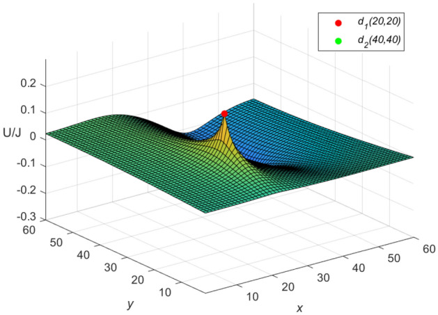
and a novel potential formula of the fan resistor network can be rewritten as

$$\begin{array}{c}\hfill \frac{{\mathcal{U}}_{m\times n}(x,y)}{J}=\frac{4r}{2m+1}\sum _{\iota =1}^m\frac{{\sum }_{s=1}^h{\epsilon }_{x_s,x}^{(\iota )}{S}_{y_1,\iota }-{\epsilon }_{x_2,x}^{(\iota )}{S}_{y_2,\iota }}{({\omega }_{\iota }-2)U_n^{(\iota )}}{S}_{y,\iota },\end{array}$$ 63

where ${\mu }_{x_s,x}^{(\iota )}$, ${\epsilon }_{x_s,x}^{(\iota )}$, $S_{y_s,\iota }$ and $U_v^{(\iota )}$ are same as Eqs. (9), (11), (12) and (14), respectively.

Let $m=n=60,J=10,x_1=y_1=20,x_2=y_2=40$, $r_0=r=1$, and $h=10$ in Eqs. (62) and (63), respectively. Then an idiosyncratic potential formula of the cobweb resistor network is represented by

$$\begin{array}{c}\hfill \frac{{\mathbf{U}}_{m\times n}(x,y)}{J}=\frac{4}{121}\sum _{\iota =1}^{60}\frac{{\sum }_{s=1}^{10}{\mu }_{x_s,x}^{(\iota )}{S}_{20,\iota }-{\mu }_{40,x}^{(\iota )}{S}_{40,\iota }}{U_{60}^{(\iota )}-U_{58}^{(\iota )}-2}{S}_{y,\iota },\end{array}$$ 64

and an idiosyncratic potential formula of the fan resistor network is represented by

$$\begin{array}{c}\hfill \frac{{\mathcal{U}}_{m\times n}(x,y)}{J}=\frac{4}{121}\sum _{\iota =1}^{60}\frac{{\sum }_{s=1}^{10}{\epsilon }_{x_s,x}^{(\iota )}{S}_{20,\iota }-{\epsilon }_{40,x}^{(\iota )}{S}_{40,\iota }}{({\omega }_{\iota }-2)U_{60}^{(\iota )}}{S}_{y,\iota },\end{array}$$ 65

$$\begin{array}{c}\hfill S_{40,\iota }=sin\left(\frac{(80\iota -40)\pi }{121}\right),\end{array}$$ 66

where ${\mu }_{40,x}^{(\iota )}$, ${\epsilon }_{40,x}^{(\iota )}$, ${\omega }_{\iota }$, $S_{20,\iota }$ and $S_{y,\iota }$ are expressed in Eqs. (59), (61), (52), (53) and (55), respectively, with $v=61-|s-x|,61-|40-x|,59-|s-x|,59-|40-x|,|s-x|-1,|40-x|-1,60-s-x,58-s-x,20-x,18-x,60,58,-0.5,s=1,2,\dots ,10.\iota =1,2,\dots ,60$.

And the three-dimensional dynamic views for the generative process of the potential graph are shown in Figs. 7 and 8 by Matlab.

Figure 7.

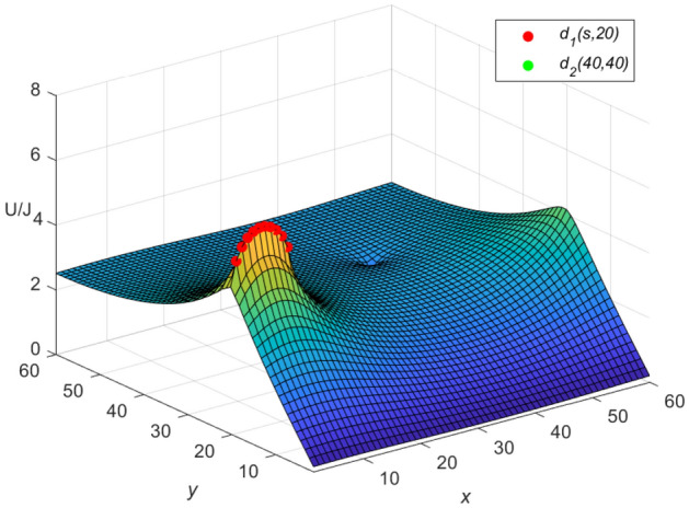
The potential graph for ${\mathbf{U}}_{60\times 60}(x,y)/J$ with the cobweb resistor network in Eq. (64).

Figure 8.

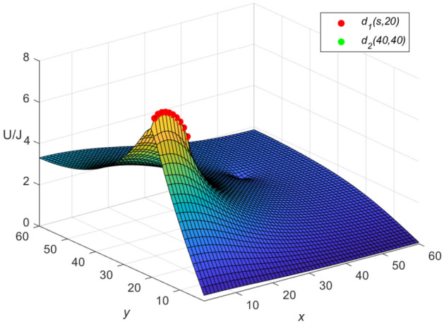
The potential graph for ${\mathcal{U}}_{60\times 60}(x,y)/J$ with the fan resistor network in Eq. (65).

Idiosyncratic potential formulas with the change of resistivity h ($h=\frac{r}{r_0}$) in resistor network

This section discusses the effect of changes in resistivity h in the resistor network on the potential formulas as reflected in the three-dimensional dynamic view.

Let $m=n=60,J=10,x_1=y_1=20,x_2=y_2=40$, and $r=1$ in Eqs. (8) and (10), respectively. Then an idiosyncratic potential formula of the cobweb resistor network is expressed by

$$\begin{array}{c}\hfill \frac{{\mathbf{U}}_{60\times 60}(x,y)}{J}=\frac{4}{121}\sum _{\iota =1}^{60}\frac{{\mu }_{20,x}^{(\iota )}{S}_{20,\iota }-{\mu }_{40,x}^{(\iota )}{S}_{40,\iota }}{U_{60}^{(\iota )}-U_{58}^{(\iota )}-2}{S}_{y,\iota },\end{array}$$ 67

and an idiosyncratic potential formula of the fan resistor network is expressed by

$$\begin{array}{c}\hfill \frac{{\mathcal{U}}_{60\times 60}(x,y)}{J}=\frac{4}{121}\sum _{\iota =1}^{60}\frac{{\epsilon }_{20,x}^{(\iota )}{S}_{20,\iota }-{\epsilon }_{40,x}^{(\iota )}{S}_{40,\iota }}{({\omega }_{\iota }-2)U_{60}^{(\iota )}}{S}_{y,\iota },\end{array}$$ 68

where ${\mu }_{20,x}^{(\iota )}$, ${\mu }_{40,x}^{(\iota )}$, ${\epsilon }_{20,x}^{(\iota )}$, ${\epsilon }_{40,x}^{(\iota )}$, $S_{20,\iota }$, $S_{40,\iota }$ and $S_{y,\iota }$ are expressed in Eqs. (50), (59), (51), (61), (53), (66) and (55), respectively.

Idiosyncratic potential formula 4. When $r_0=10$, $h=0.1$ is got, as h changes, ${\omega }_{\iota }$ and ${\varphi }_{\iota }$ are obtained as follows, respectively

$$\begin{array}{cc}\hfill {\omega }_{\iota }& =2.2-0.2cos\frac{(2\iota -1)\pi }{121},\hfill \\ \hfill cosh{\varphi }_{\iota }& =1.1-0.1cos\frac{(2\iota -1)\pi }{121}.\hfill \end{array}$$ 69

Equation (69) is combined with Eqs. (67) and (68), respectively, and the three-dimensional dynamic views for the generative process of the potential graph are shown in Figs. 9 and 10, respectively.

Figure 9.

The potential graph for ${\mathbf{U}}_{60\times 60}(x,y)/J$ with the cobweb resistor network by Eq. (67).

Figure 10.

The potential graph for ${\mathcal{U}}_{60\times 60}(x,y)/J$ with the fan resistor network by Eq. (68).

Idiosyncratic potential formula 5. When $r_0=1$, $h=1$ is got, as h changes, ${\omega }_{\iota }$ and ${\varphi }_{\iota }$ are obtained as follows, respectively

$$\begin{array}{cc}\hfill {\omega }_{\iota }& =4-2cos\frac{(2\iota -1)\pi }{121},\hfill \\ \hfill cosh{\varphi }_{\iota }& =2-cos\frac{(2\iota -1)\pi }{121}.\hfill \end{array}$$ 70

Equation (70) is combined with Eqs. (67) (68), respectively, and the three-dimensional dynamic views for the generative process of the potential graph are shown in Figs. 11 and 12, respectively.

Figure 11.

The potential graph for ${\mathbf{U}}_{60\times 60}(x,y)/J$ with the cobweb resistor network by Eq. (67).

Figure 12.

The potential graph for ${\mathcal{U}}_{60\times 60}(x,y)/J$ with the fan resistor network by Eq. (68).

Idiosyncratic potential formula 6. When $r_0=0.1$, $h=10$ is got, as h changes, ${\omega }_{\iota }$ and ${\varphi }_{\iota }$ are obtained as follows, respectively

$$\begin{array}{cc}\hfill {\omega }_{\iota }& =22-20cos\frac{(2\iota -1)\pi }{121},\hfill \\ \hfill cosh{\varphi }_{\iota }& =11-10cos\frac{(2\iota -1)\pi }{121}.\hfill \end{array}$$ 71

Equation (71) is combined with Eqs. (67) and (68), respectively, and the three-dimensional dynamic views for the generative process of the potential graph are shown in Figs. 13 and 14, respectively.

Figure 13.

The potential graph for ${\mathbf{U}}_{60\times 60}(x,y)/J$ with the cobweb resistor network by Eq. (67).

Figure 14.

The potential graph for ${\mathcal{U}}_{60\times 60}(x,y)/J$ with the fan resistor network by Eq. (68).

Numerical algorithms for computing potential

Combining the DST-VI and Eqs. (30), (31), (32), (33), (34), this chapter provides two numerical algorithms to achieve fast calculation of large-scale potential for the resistor network. The numerical algorithm obtains similar results to the potential formulas (8) and (10).

Remark 5

As is well-known, the Algorithm 1 is a tridiagonal matrix-vector multiplication, which the computational complexity is O(n). Moreover, one DST-VI needs $2n{log}_{2}n+O(n)$ real arithmetic operations⁶⁸. So the Algorithm 2 composed of Algorithm 1 and two DST-VI, and it’s computational complexity is $4n{log}_{2}n+O(n)$. Analogous, the computational complexity of Algorithms 3 is also $4n{log}_{2}n+O(n)$. According to the above Algorithms 2 and Algorithms 3, two instances are used to display the iterative effect of large-scale data graphically in the following.

Let $m=400$ and $n=10$, the current J flows from the $d_1(x_1,y_1)$ point, $x_1=3,y_1=150$, and out from the $d_2(x_2,y_2)$ point, $x_2=7,y_2=350$. $r=1$, $r_0=100$, and $J=10$. The fast algorithm of cobweb resistor network is shown in Fig. 15, and the fast algorithm of fan resistor network is shown in Fig. 16.

Figure 15.

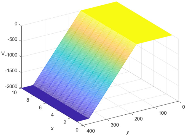
A 3D image display for the fast Algorithm 2 of ${\mathbf{U}}_{400\times 10}(x,y)/J$ on the cobweb resistor network.

Figure 16.

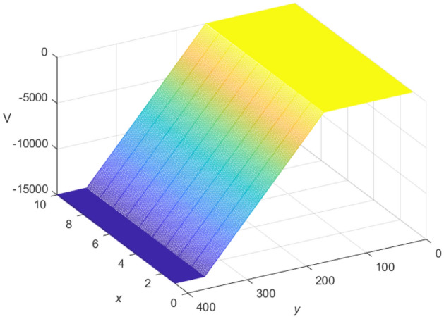
A 3D image display for the fast Algorithm 3 of ${\mathcal{U}}_{400\times 10}(x,y)/J$ on the fan resistor network.

Efficiency of calculation method

On the $m\times n$ scale resistor network models, $(x_1,y_1)$ refers to the input point of the current and $(x_2,y_2)$ refers to the output point of the current. We give a comparison of calculation efficiency for the calculating potential in three different methods. “Time” is the total CPU time in seconds, $t_1$, $t_2$ and $t_3$ denote CPU times of the potential computed by formulas (1), (3), formulas (8), (10) and Algorithm 2, 3, respectively.

The experiment is completed under the environmental conditions of CPU model AMD R9-5900HX, CPU frequency 3.30 GHz, and Matlab version is R2020b. $``m\times n"$ is the number of nodes in the resistor network., $``-"$ denotes the operation time more than 1200s or beyond the memory limit of Matlab.

Remark 6

Tables 1, 3, 5 show the calculation time of cobweb resistor network with different square and rectangular sizes at different resistivity. The optimized potential formula (8) has faster operation speed.

Table 1.

The comparison of calculation efficiency for potential formulas (1) and (8).

$m\times n$	$(x_1,y_1)$	$(x_2,y_2)$	$r/r_0$	$t_1$	$t_2$
$100\times 100$	(40 , 40)	(80 , 80)	1	0.139	0.029
$200\times 200$	(40 , 40)	(180 , 180)	1	0.923	0.121
$300\times 300$	(40 , 40)	(180 , 180)	1	2.817	0.340
$400\times 400$	(40 , 40)	(180 , 180)	1	7.685	1.649
$800\times 100$	(40 , 40)	(80 , 80)	1	6.652	0.874
$800\times 200$	(40 , 40)	(180 , 180)	1	15.269	3.510

Table 3.

The comparison of calculation efficiency for potential formulas (1) and (8).

$m\times n$	$(x_1,y_1)$	$(x_2,y_2)$	$r/r_0$	$t_1$	$t_2$
$400\times 400$	(40 , 40)	(180 , 180)	0.1	7.626	1.760
$500\times 500$	(40 , 40)	(180 , 180)	0.1	14.666	3.001
$600\times 600$	(40 , 40)	(180 , 180)	0.1	25.365	4.932
$1100\times 1100$	(40 , 40)	(180 , 180)	0.1	159.767	34.444
$1000\times 400$	(40 , 40)	(180 , 180)	0.1	47.323	9.187
$1000\times 500$	(40 , 40)	(180 , 180)	0.1	59.539	11.613

Table 5.

The comparison of calculation efficiency for potential formulas (1) and (8).

$m\times n$	$(x_1,y_1)$	$(x_2,y_2)$	$r/r_0$	$t_1$	$t_2$
$1000\times 1000$	(40 , 40)	(580 , 580)	0.01	120.787	25.788
$1500\times 1500$	(40 , 40)	(580 , 580)	0.01	405.983	92.694
$1800\times 1800$	(40 , 40)	(580 , 580)	0.01	700.525	159.449
$2000\times 2000$	(40 , 40)	(580 , 580)	0.01	958.713	217.022
$1500\times 1000$	(40 , 40)	(580 , 580)	0.01	270.714	61.578
$2000\times 1000$	(40 , 40)	(580 , 580)	0.01	480.070	110.790

Remark 7

Tables 2, 4, 6 show the calculation time of fan resistor network with different square and rectangular sizes at different resistivity. The optimized potential formula (10) has faster operation speed.

Table 2.

The comparison of calculation efficiency for potential formulas (3) and (10).

$m\times n$	$(x_1,y_1)$	$(x_2,y_2)$	$r/r_0$	$t_1$	$t_2$
$100\times 100$	(40 , 40)	(80 , 80)	1	0.271	0.045
$200\times 200$	(40 , 40)	(180 , 180)	1	1.667	0.244
$300\times 300$	(40 , 40)	(180 , 180)	1	–	0.631
$400\times 400$	(40 , 40)	(180 , 180)	1	–	2.964
$800\times 100$	(40 , 40)	(80 , 80)	1	13.210	1.546
$800\times 200$	(40 , 40)	(180 , 180)	1	30.351	5.925

Table 4.

The comparison of calculation efficiency for potential formulas (3) and (10).

$m\times n$	$(x_1,y_1)$	$(x_2,y_2)$	$r/r_0$	$t_1$	$t_2$
$400\times 400$	(40 , 40)	(180 , 180)	0.1	14.962	3.016
$500\times 500$	(40 , 40)	(180 , 180)	0.1	28.453	5.325
$600\times 600$	(40 , 40)	(180 , 180)	0.1	–	9.052
$1100\times 1100$	(40 , 40)	(180 , 180)	0.1	–	63.093
$1000\times 400$	(40 , 40)	(180 , 180)	0.1	91.827	16.498
$1000\times 500$	(40 , 40)	(180 , 180)	0.1	118.262	20.461

Table 6.

The comparison of calculation efficiency for potential formulas (3) and (10).

$m\times n$	$(x_1,y_1)$	$(x_2,y_2)$	$r/r_0$	$t_1$	$t_2$
$1000\times 1000$	(40 , 40)	(580 , 580)	0.01	234.791	46.840
$1500\times 1500$	(40 , 40)	(580 , 580)	0.01	792.929	171.828
$1800\times 1800$	(40 , 40)	(580 , 580)	0.01	1373.612	308.328
$2000\times 2000$	(40 , 40)	(580 , 580)	0.01	–	410.130
$1500\times 1000$	(40 , 40)	(580 , 580)	0.01	528.783	114.033
$2000\times 1000$	(40 , 40)	(580 , 580)	0.01	943.748	208.219

Remark 8

Table 7 shows the efficiency of the potential formula (1), formula (8) and the Algorithm 2 for calculating the potential. Algorithm 2 not only realizes large-scale calculation, but also has shorter calculation time in calculating cobweb resistor network.

Table 7.

Comparison of the efficiency for potential formulas (1), (8) and Algorithm 2.

$m\times n$	$(x_1,y_1)$	$(x_2,y_2)$	$r/r_0$	$t_1$	$t_2$	$t_3$
$100\times 10$	(3 , 30)	(5 , 50)	0.01	0.031	0.013	0.013
$1000\times 10$	(3 , 300)	(5 , 500)	0.01	1.144	0.213	0.033
$10000\times 10$	(3 , 3000)	(5 , 5000)	0.01	105.350	11.588	1.098
$20000\times 10$	(3 , 3000)	(5 , 5000)	0.01	474.890	93.546	4.156
$30000\times 10$	(3 , 3000)	(5 , 5000)	0.01	1043.302	204.098	8.369
$40000\times 10$	(3 , 3000)	(5 , 5000)	0.01	1857.076	358.305	19.710

Remark 9

Table 8 shows the efficiency of the potential formula (3), formula (10) and the Algorithm 3 for calculating the potential. Algorithm 3 not only realizes large-scale calculation, but also has shorter calculation time in calculating fan resistor network.

Table 8.

Comparison of the efficiency for potential formulas (3), (10) and Algorithm 3.

$m\times n$	$(x_1,y_1)$	$(x_2,y_2)$	$r/r_0$	$t_1$	$t_2$	$t_3$
$100\times 10$	(3 , 30)	(5 , 50)	0.01	0.035	0.017	0.013
$1000\times 10$	(3 , 300)	(5 , 500)	0.01	1.188	0.388	0.050
$10000\times 10$	(3 , 3000)	(5 , 5000)	0.01	106.246	21.425	1.014
$20000\times 10$	(3 , 3000)	(5 , 5000)	0.01	468.767	175.736	3.465
$30000\times 10$	(3 , 3000)	(5 , 5000)	0.01	1041.555	365.012	7.998
$40000\times 10$	(3 , 3000)	(5 , 5000)	0.01	1858.145	637.289	19.353

Conclusion

In this paper, based on the RT-V method, the accurate potential formulas of the $m\times n$ cobweb resistor network and the $m\times n$ fan resistor network¹ are improved. The potential formula is represented by the Chebyshev polynomial of the second class and the tridiagonal matrix is diagonalized by the DST-VI method, which realizes the high efficiency of the numerical simulation of the potential formula. The changes of variables in the potential formula are analyzed, and the corresponding three-dimensional view is drawn to show the influence of variable changes on the image. Then we design a fast algorithm for the resistor network potential to achieve fast calculation in the case of large-scale resistor networks. Finally, we show the calculation time of different calculation methods under different scale resistor networks, and the comparison shows the efficiency of the improved numerical simulation calculation.

Author contributions

Zheng, Yan-Peng and Jiang, Xiao-Yu conceived the project, performed and analyzed formulae calculations. Zhao, Wen-Jie validated the correctness of the formula calculation, and realized the numerical simulation and graph drawing. Jiang, Zhao-Lin present the fast algorithm of computing potential. All authors contributed equally to the manuscript.

Data availability

All data generated or analysed during this study are included in this article and its supplementary information files.

Competing interests

The authors declare no competing interests.

References

- 1.Tan Z-Z. Recursion-transform method and potential formulae of the cobweb and fan networks. Chin. Phys. B. 2017;26(9):090503. doi: 10.1088/1674-1056/26/9/090503. [DOI] [Google Scholar]
- 2.Hadad, Y., Soric, J. C., Khanikaev, A. B. & Al, A. Self-induced topological protection in nonlinear circuit arrays. Nat. Electron.1, 178–182 (2018).
- 3.Zhang D, Yang B, Jin Y-B, Xiao B, Xian G, Xue X-L, Li Y. Impact damage localization and mode identification of CFRPs panels using an electric resistance change method. Compos. Struct. 2021;276:114587. doi: 10.1016/j.compstruct.2021.114587. [DOI] [Google Scholar]
- 4.Kirchhoff G. Ueber die Aufölsung der Gleichungen, auf welche man bei der Untersuchung der linearen Vertheilung galvanischer Ströme geführt wird. Ann. Phys. 1847;148:497–508. doi: 10.1002/andp.18471481202. [DOI] [Google Scholar]
- 5.Winstead V, Demarco CL. Network essentiality. IEEE Trans. Circuits-I. 2012;60(3):703–709. [Google Scholar]
- 6.Ferri G, Antonini G. Ladder-network-based model for interconnects and transmission lines time delay and cutoff frequency determination. J. Circuit. Syst. Comput. 2007;16:489–505. doi: 10.1142/S0218126607003794. [DOI] [Google Scholar]
- 7.Owaidat MQ, Hijjawi RS, Khalifeh JM. Network with two extra interstitial resistors. Int. J. Theor. Phys. 2012;51:3152–3159. doi: 10.1007/s10773-012-1196-5. [DOI] [Google Scholar]
- 8.Kirkpatrick S. Percolation and Conduction. Rev. Mod. Phys. 1973;45:497–508. doi: 10.1103/RevModPhys.45.574. [DOI] [Google Scholar]
- 9.Katsura S, Inawashiro S. Lattice Green’s functions for the rectangular and the square lattices at arbitrary points. J. Math. Phys. 1971;12:1622. doi: 10.1063/1.1665785. [DOI] [Google Scholar]
- 10.Pennetta C, Alfinito E, Reggiani L, Fantini F, DeMunari I, Scorzoni A. Biased resistor network model for electromigration failure and related phenomena in metallic lines. Phys. Rev. B. 2004;70:174305. doi: 10.1103/PhysRevB.70.174305. [DOI] [Google Scholar]
- 11.Kook W. Combinatorial Green’s function of a graph and applications to networks. Adv. Appl. Math. 2011;46:417–423. doi: 10.1016/j.aam.2010.10.006. [DOI] [Google Scholar]
- 12.Shi Y, Jin L, Li S, Li J, Qiang J-P, Gerontitis DK. Novel discrete-time recurrent neural networks handling discrete-form time-variant multi-augmented Sylvester matrix problems and manipulator application. IEEE Trans. Neur. Net. Lear. 2022;33(2):587–599. doi: 10.1109/TNNLS.2020.3028136. [DOI] [PubMed] [Google Scholar]
- 13.Shi, Y., Zhao, W.-H., Li, S., Li, B. & Sun, X.-B. Novel discrete-time recurrent neural network for robot manipulator: a direct discretization technical route. IEEE Trans. Neur. Net. Lear. (2021). 10.1109/TNNLS.2021.3108050 [DOI] [PubMed]
- 14.Liu K-P, Liu Y-B, Zhang Y, Wei L, Sun Z-B, Jin L. Five-step discrete-time noise-tolerant zeroing neural network model for time-varying matrix inversion with application to manipulator motion generation. Eng. Appl. Artif. Intel. 2021;103:104306. doi: 10.1016/j.engappai.2021.104306. [DOI] [Google Scholar]
- 15.Sun Z-B, Wang G, Jin L, Cheng C, Zhang B-C, Yu J-Z. Noise-suppressing zeroing neural network for online solving time-varying matrix square roots problems: A control-theoretic approach. Expert. Syst. Appl. 2022;192:116272. doi: 10.1016/j.eswa.2021.116272. [DOI] [Google Scholar]
- 16.Jin L, Qi Y-M, Luo X, Li S, Shang M-S. Distributed competition of multi-robot coordination under variable and switching topologies. IEEE Trans. Autom. Sci. Eng. 2022;19(4):3575–3586. doi: 10.1109/TASE.2021.3126385. [DOI] [Google Scholar]
- 17.Jin L, Zhang Y-N, Li S, Zhang Y-Y. Modified ZNN for time-varying quadratic programming with inherent tolerance to noises and its application to kinematic redundancy resolution of robot manipulators. IEEE T. Ind. Electron. 2016;63(11):6978–6988. doi: 10.1109/TIE.2016.2590379. [DOI] [Google Scholar]
- 18.Jin L, Zheng X, Luo X. Neural dynamics for distributed collaborative control of manipulators with time delays. IEEE-CAA J. Autom. 2022;9(5):854–863. [Google Scholar]
- 19.Klein, D. J., & Randi, M. Resistance distance. J. Math. Chem.12, 81–95 (1993).
- 20.Cserti J. Application of the lattice Green’s function for calculating the resistance of an infinite network of resistors. Am. J. Phys. 2000;68:896–906. doi: 10.1119/1.1285881. [DOI] [Google Scholar]
- 21.Giordano S. Disordered lattice networks: general theory and simulations. Int. J. Circ. Theor. App. 2005;33:519–540. doi: 10.1002/cta.335. [DOI] [Google Scholar]
- 22.Wu FY. Theory of resistor networks: The two-point resistance. J. Phys. A: Math. Gen. 2004;37:6653. doi: 10.1088/0305-4470/37/26/004. [DOI] [Google Scholar]
- 23.Tzeng WJ, Wu FY. Theory of impedance networks: The two-point impedance and LC resonances. J. Phys. A: Math. Gen. 2006;39:8579. doi: 10.1088/0305-4470/39/27/002. [DOI] [Google Scholar]
- 24.Essam JW, Wu FY. The exact evaluation of the corner-to-corner resistance of an resistor network: Asymptotic expansion. J. Phys. A : Math. Theor. 2008;42:025205. doi: 10.1088/1751-8113/42/2/025205. [DOI] [Google Scholar]
- 25.Izmailian NS, Huang M-C. Asymptotic expansion for the resistance between two maximum separated nodes on an by resistor network. Phys. Rev. E. 2010;82:011125. doi: 10.1103/PhysRevE.82.011125. [DOI] [PubMed] [Google Scholar]
- 26.Lai M-C, Wang W-C. Fast direct solvers for Poisson equation on 2D polar and spherical geometries. Numer. Meth. Part. D. E. 2002;18:56–68. doi: 10.1002/num.1038. [DOI] [Google Scholar]
- 27.Borges L, Daripa P. A fast parallel algorithm for the Poisson equation on a disk. J. Comput. Phys. 2001;169:151–192. doi: 10.1006/jcph.2001.6720. [DOI] [Google Scholar]
- 28.Izmailian NS, Kenna R, Wu FY. The two-point resistance of a resistor network: A new formulation and application to the cobweb network. J. Phys. A: Math. Theor. 2014;47:035003. doi: 10.1088/1751-8113/47/3/035003. [DOI] [Google Scholar]
- 29.Izmailian NS, Kenna R. A generalised formulation of the Laplacian approach to resistor networks. J. Stat. Mech : Theor. E. 2014;9:1742–5468. [Google Scholar]
- 30.Izmailian NS, Kenna R. The two-point resistance of fan networks. Chin. J. Phys. 2015;53(2):040703. [Google Scholar]
- 31.Chair N. Trigonometrical sums connected with the chiral Potts model, Verlinde dimension formula, two-dimensional resistor network, and number theory. Ann. Phys. 2014;341:56–76. doi: 10.1016/j.aop.2013.11.012. [DOI] [Google Scholar]
- 32.Chair N. The effective resistance of the N-cycle graph with four nearest neighbors. J. Stat. Phys. 2014;154:1177–1190. doi: 10.1007/s10955-014-0916-z. [DOI] [Google Scholar]
- 33.Tan Z-Z, Zhou L, Yang J-H. The equivalent resistance of a cobweb network and its conjecture of an cobweb network. J. Phys. A: Math. Theor. 2013;46(19):195202. doi: 10.1088/1751-8113/46/19/195202. [DOI] [Google Scholar]
- 34.Tan Z-Z. Recursion-transform approach to compute the resistance of a resistor network with an arbitrary boundary. Chin. Phys. B. 2015;24(2):020503. doi: 10.1088/1674-1056/24/2/020503. [DOI] [Google Scholar]
- 35.Tan Z-Z. Recursion-transform method for computing resistance of the complex resistor network with three arbitrary boundaries. Phys. Rev. E. 2015;91(5):052122. doi: 10.1103/PhysRevE.91.052122. [DOI] [PubMed] [Google Scholar]
- 36.Tan Z-Z. Recursion-transform method to a non-regular cobweb with an arbitrary longitude. Sci. Rep. 2015;5:11266. doi: 10.1038/srep11266. [DOI] [PMC free article] [PubMed] [Google Scholar]
- 37.Tan Z-Z, Essam JW, Wu FY. Two-point resistance of a resistor network embedded on a globe. Phys. Rev. E. 2014;90(1):012130. doi: 10.1103/PhysRevE.90.012130. [DOI] [PubMed] [Google Scholar]
- 38.Essam JW, Tan Z-Z, Wu FY. Resistance between two nodes in general position on an fan network. Phys. Rev. E. 2014;90(3):032130. doi: 10.1103/PhysRevE.90.032130. [DOI] [PubMed] [Google Scholar]
- 39.Tan Z-Z, Fang J-H. Two-point resistance of a cobweb network with a boundary. Commun. Theor. Phys. 2015;63(1):36–44. doi: 10.1088/0253-6102/63/1/07. [DOI] [Google Scholar]
- 40.Tan Z-Z. Theory on resistance of cobweb network and its application. Int. J. Circ. Theor. Appl. 2015;43(11):1687–1702. doi: 10.1002/cta.2035. [DOI] [Google Scholar]
- 41.Tan Z-Z. Two-point resistance of a non-regular cylindrical network with a zero resistor axis and two arbitrary boundaries. Commun. Theor. Phys. 2017;67(3):280–288. doi: 10.1088/0253-6102/67/3/280. [DOI] [Google Scholar]
- 42.Tan Z-Z. Two-point resistance of an resistor network with an arbitrary boundary and its application in RLC network. Chin. Phys. B. 2016;25(5):050504. doi: 10.1088/1674-1056/25/5/050504. [DOI] [Google Scholar]
- 43.Tan Z, Tan Z-Z, Chen J. Potential formula of the nonregular fan network and its application. Sci. Rep. 2018;8:5798. doi: 10.1038/s41598-018-24164-x. [DOI] [PMC free article] [PubMed] [Google Scholar]
- 44.Tan Z, Tan Z-Z. Potential formula of an globe network and its application. Sci. Rep. 2018;8(1):9937. doi: 10.1038/s41598-018-27402-4. [DOI] [PMC free article] [PubMed] [Google Scholar]
- 45.Tan Z-Z, Tan Z. Electrical properties of an arbitrary rectangular network. Acta Phys. Sin. 2020;62(2):020502. doi: 10.7498/aps.69.20191303. [DOI] [Google Scholar]
- 46.Tan Z-Z. Resistance theory for two classes of n-periodic networks. Eur. Phys. J. Plus. 2022;137(5):1–12. doi: 10.1140/epjp/s13360-022-02750-3. [DOI] [Google Scholar]
- 47.Tan Z-Z, Tan Z. Electrical properties of cylindrical network. Chin. Phys. B. 2020;29(8):080503. doi: 10.1088/1674-1056/ab96a7. [DOI] [Google Scholar]
- 48.Tan Z-Z, Tan Z. The basic principle of resistor networks. Commun. Theor. Phys. 2020;72(5):055001. doi: 10.1088/1572-9494/ab7702. [DOI] [Google Scholar]
- 49.Fang X-Y, Tan Z-Z. Circuit network theory of n-horizontal bridge structure. Sci. Rep. 2022;12(1):6158. doi: 10.1038/s41598-022-09841-2. [DOI] [PMC free article] [PubMed] [Google Scholar]
- 50.Tan Z-Z. Electrical property of an apple surface network. Results Phys. 2023;47:106361. doi: 10.1016/j.rinp.2023.106361. [DOI] [Google Scholar]
- 51.Luo X-L, Tan Z-Z. Fractional circuit network theory with n-V-structure. Phys. Scr. 2023;98(4):045224. doi: 10.1088/1402-4896/acc491. [DOI] [Google Scholar]
- 52.Tan Z-Z. Theory of an apple surface network with special boundary. Commun. Theor. Phys. 2023;75(6):065701. doi: 10.1088/1572-9494/accb82. [DOI] [Google Scholar]
- 53.Zhou S, Wang Z-X, Zhao Y-Q, Tan Z-Z. Electrical properties of a generalized resistor network. Commun. Theor. Phys. 2023;75:075701. doi: 10.1088/1572-9494/acd2b9. [DOI] [Google Scholar]
- 54.Fu Y-R, Jiang X-Y, Jiang Z-L, Jhang S. Properties of a class of perturbed Toeplitz periodic tridiagonal matrices. Comp. Appl. Math. 2020;39:1–19. doi: 10.1007/s40314-020-01171-1. [DOI] [Google Scholar]
- 55.Fu Y-R, Jiang X-Y, Jiang Z-L, Jhang S. Inverses and eigenpairs of tridiagonal Toeplitz matrix with opposite-bordered rows. J. Appl. Anal. Comput. 2020;10(4):1599–1613. [Google Scholar]
- 56.Fu Y-R, Jiang X-Y, Jiang Z-L, Jhang S. Analytic determinants and inverses of Toeplitz and Hankel tridiagonal matrices with perturbed columns. Spec. Matrices. 2020;8:131–143. doi: 10.1515/spma-2020-0012. [DOI] [Google Scholar]
- 57.Wei Y-L, Zheng Y-P, Jiang Z-L, Shon S. The inverses and eigenpairs of tridiagonal Toeplitz matrices with perturbed rows. J. Appl. Math. Comput. 2022;68:623–636. doi: 10.1007/s12190-021-01532-x. [DOI] [Google Scholar]
- 58.Wei Y-L, Jiang X-Y, Jiang Z-L, Shon S. On inverses and eigenpairs of periodic tridiagonal Toeplitz matrices with perturbed corners. J. Appl. Anal. Comput. 2020;10(1):178–191. [Google Scholar]
- 59.Wei Y-L, Zheng Y-P, Jiang Z-L, Shon S. A study of determinants and inverses for periodic tridiagonal Toeplitz matrices with perturbed corners involving Mersenne numbers. Mathematics. 2019;7(10):893. doi: 10.3390/math7100893. [DOI] [Google Scholar]
- 60.Wei Y-L, Jiang X-Y, Jiang Z-L, Shon S. Determinants and inverses of perturbed periodic tridiagonal Toeplitz matrices. Adv. Differ. Equ. 2019;2019(1):410. doi: 10.1186/s13662-019-2335-6. [DOI] [Google Scholar]
- 61.Zhou Y-F, Zheng Y-P, Jiang X-Y, Jiang Z-L. Fast algorithm and new potential formula represented by Chebyshev polynomials for an globe network. Sci. Rep. 2022;12(1):21260. doi: 10.1038/s41598-022-25724-y. [DOI] [PMC free article] [PubMed] [Google Scholar]
- 62.Mason, J. C. & Handscomb, D. C. Chebyshev Polynomials. (Chapman & Hall/CRC, 2002).
- 63.Udrea, G. A note on the sequence of A.F. Horadam. Port. Math.53, 143–156 (1996).
- 64.Garcia SR, Yih S. Supercharacters and the discrete Fourier, cosine, and sine transforms. Commun. Algebra. 2018;46(9):3745–3765. doi: 10.1080/00927872.2018.1424866. [DOI] [Google Scholar]
- 65.Sanchez V, Garcia P, Peinado AM, Segura JC, Rubio AJ. Diagonalizing properties of the discrete cosine transforms. IEEE Trans. Signal. Process. 1995;43(11):2631–2641. doi: 10.1109/78.482113. [DOI] [Google Scholar]
- 66.Strang G. The discrete cosine transform. SIAM. Rev. 1999;41(1):135–147. doi: 10.1137/S0036144598336745. [DOI] [Google Scholar]
- 67.Liu Z, Chen S, Xu W, Zhang Y. The eigen-structures of real (skew) circulant matrices with some applications. Comput. Appl. Math. 2019;38:178. doi: 10.1007/s40314-019-0971-9. [DOI] [Google Scholar]
- 68.Yip, P. C. & Rao, K. R. DIF algorithms for DCT and DST. IEEE Int. Conf. Acoust. Speech and Signal Processing. 776–779. 10.1109/ICASSP.1985.1168246 (1985). [DOI]
Associated Data
This section collects any data citations, data availability statements, or supplementary materials included in this article.
Data Availability Statement