Convex optimization algorithms in medical image reconstruction–in the age of AI

Abstract

The past decade has seen the rapid growth of model based image reconstruction (MBIR) algorithms, which are often applications or adaptations of convex optimization algorithms from the optimization community. We review some state-of-the-art algorithms that have enjoyed wide popularity in medical image reconstruction, emphasize known connections between different algorithms, and discuss practical issues such as computation and memory cost. More recently, deep learning (DL) has forayed into medical imaging, where the latest development tries to exploit the synergy between DL and MBIR to elevate the MBIR’s performance. We present existing approaches and emerging trends in DL-enhanced MBIR methods, with particular attention to the underlying role of convexity and convex algorithms on network architecture. We also discuss how convexity can be employed to improve the generalizability and representation power of DL networks in general.

1. Introduction

The last decade has witnessed intense research activities in developing model based image reconstruction (MBIR) methods for CT, MR, PET, and SPECT. Numerous publications have documented the benefits of these MBIR methods, ranging from mitigating image artifacts and improving image quality in general, to reducing radiation dose in CT applications. The MBIR problem is often formulated as an optimization problem, where a scalar objective function, consisting of a data fitting term and a regularizer, is to be minimized with respect to the unknown image. Driven by such large scale and data intensive applications, the same period of time has also seen intense research on developing convex optimization algorithms in the mathematical community. The infusion of concepts in convex optimization into the imaging community has sparked many new research directions, such as MBIR algorithms with fast convergence properties, and novel regularizer designs that better capture a priori image information.

More recently, deep learning (DL) methods have achieved super-human performance in many complex real world tasks. Their quick adoption and adaptation for solving medical imaging problems have also been fruitful. The number of publications on DL approaches for inverse problems has exploded. As evidence of such fast-paced development, a number of special issues (Greenspan et al 2016, Wang et al 2018, Duncan et al 2019) and review articles (McCann et al 2017, Lucas et al 2018, Willemink and Noël 2019, Lell and Kachelrie 2020) have been produced to summarize the current state-of-the-art.

Many articles have discussed the strengths and challenges of AI and DL in general, and others have debated about their role and future in medical imaging. A cautionary view is that DL should be acknowledged for its power, but it is not the magic bullet that solves all problems. It is plausible that DL can work synergistically with conventional methods, e.g., convex optimization: where the conventional methods excel may be where DL falters. For example, DL is often criticized for low interpretability. Convex optimization, on the other hand, is well known for its rich structure and can be used to encode structural information and improve interpretability when combined with DL networks. DL is also data hungry (Marcus 2018); it requires a large amount of training data with known ground truth for either training or evaluation. DL can be used to enhance the performance of conventional MBIR methods, which then in turn produce high quality ground truth labels for DL training.

With that as the background, in this paper we review the basic concepts in convexoptimization, discuss popular first order algorithms that have seen wide applications inMBIR problems, and use example applications in the literature to showcase the relevance of convexity in the age of AI and DL. The following is an outline of the main content of the paper.

• section 2: Elements in convex optimization

• section 3: Deterministic first order algorithms for convex optimization

• section 4: Stochastic first order algorithms for convex optimization

• section 5: Convexity in nonconvex optimization

• section 6: Synergistic integration of convexity, image reconstruction, and DL

• section 7: Conclusions

• section 8: Appendix – additional topics such as Bregman distance, the relative smoothness of the Poisson likelihood, and some computational examples.

2. Elements in convex optimization

We first introduce common notation that is used throughout the paper. Notation that is only relevant to a particular section will be introduced locally. We then explain basic concepts and results from convex analysis that are helpful to understand the content of the paper, especially sections 3,4, and 5.

2.1. Notation

We denote by ${\iota }_C$ the indicator function of a set $C$, i.e., ${\iota }_C\left(x\right)=0$ if $x\in C$, and $+\mathrm{\infty }$ otherwise. A set $C\subset R^n$ is convex if and only if (iff) for all $x_1,x_2\in C,\alpha x_1+(1-\alpha )x_2\in C$. The domain of a function $f:R^n\to R\cup \{+\mathrm{\infty }\}$ is defined as $\mathrm{d}\mathrm{o}\mathrm{m}f=\{x\mid f(x)<\mathrm{\infty }\}$; a function $f$ is proper if its domain is nonempty. A function $f$ is closed if its epigraph epi $f=\left\{(x,t)\in R^{n+1}\mid f\left(x\right)⩽t,x\in \mathrm{d}\mathrm{o}\mathrm{m}f\right\}$ is closed. A function $f$ is lower semicontinuous if its epigraph is closed (Bauschke et al 2011), lemma 1.24. A function $f:C\subset R^n\to R\cup \{+\mathrm{\infty }\}$ is convex if $C\subset R^n$ is a convex set, and for $\alpha \in [0,1]$, and $x_1,x_2\in C,f\left(\alpha x_1+(1-\alpha )x_2\right)⩽\alpha f\left(x_1\right)+(1-\alpha )f\left(x_2\right)$. We use the abbreviation CCP to denote a function $f$ that is convex, closed, and proper. For convenience, we may refer to such functions simply as convex.

We denote by $⟨\cdot ,\cdot ⟩$ the inner product of two vectors, i.e., $⟨a,b⟩={\sum }_i{a}_i{b}_i$, for $a,b\in R^n$. The inner product induced norm is denoted by $\parallel \cdot {\parallel }_2$ or simply $\parallel \cdot \parallel$, i.e., $\parallel x\parallel =\sqrt{⟨x,x⟩}$. If not stated otherwise, the norm we use in this paper is the 2-norm.

2.2. Basic definitions and properties

First order algorithms are categorized according to the type of objective functions they are designed for. Among the different types, smooth objective functions are the most common assumption and possibly the easiest to work with. Let $Q\subseteq R^d$. If a convex function $f$ is differentiable and its gradient $\nabla f$ is Lipschitz continuous, i.e., there exists a constant $L>0$ such that

$$\Vert \nabla f(x)-\nabla f(y)\Vert ⩽L\Vert x-y\Vert ,\forall x,y\in Q$$ (2.1)

then $f$ is $L$-smooth on $Q$. From (Nesterov et al 2018), theorem 2.1.5, such functions can be equivalently characterized by

$$0⩽f(y)-\left[f(x)+\langle \nabla f(x),(y-x)\rangle \right]⩽\frac{L}{2}{\Vert y-x\Vert }^2,x,y\in Q$$ (2.2)

This relationship states that an $L$-smooth function admits a quadratic majorizer for any $x,y\in Q$. The constant $L$ in (2.2) is the gradient Lipschitz constant.

A function $f:Q\subseteq R^d\to R\cup \{+\mathrm{\infty }\}$ is $\sigma$-strongly convex if

$$f\left(\alpha x_1+(1-\alpha )x_2\right)⩽\alpha f\left(x_1\right)+(1-\alpha )f\left(x_2\right)-\frac{1}{2}\alpha (1-\alpha )\sigma {\Vert x_1-x_2\Vert }^2,$$ (2.3)

for $\alpha \in [0,1]$, and for all $x_1,x_2\in Q$. When the function $f$ is differentiable, an alternative characterization of $\sigma$-strongly convex functions is given by

$$f(x)+\langle \nabla f(x),y-x\rangle +\frac{1}{2}\sigma {\Vert x-y\Vert }^2⩽f(y)$$ (2.4)

Let $f:Q\subseteq R^d\to R\cup \{+\mathrm{\infty }\}$ be CCP, and $x\in Q$, the subdifferential of $f$ at $x$, denoted by $\partial f\left(x\right)$, is defined as:

$$\partial f(x):=\{u\in Q|f(y)⩾f(x)+\langle u,y-x\rangle ,\text{for all}y\in Q\}$$ (2.5)

Elements of the set $\partial f\left(x\right)$ are called subgradients at $x$. The subdifferential $\partial f\left(x\right)$ of a proper convex $f$ is nonempty for $x\in \mathrm{r}\mathrm{i}\mathrm{d}\mathrm{o}\mathrm{m}f$ (Bauschke et al 2011, page 228). Minimizers of a CCP $f$ can be characterized by Fermat’s rule, which states that $x$ is a minimizer of $f$ iff $0\in \partial f\left(x\right)$ (Rockafellar and Wets 2009, page 422).

The conjugate function $f^{\ast }$ of $f:R^d\to R\cup \{+\mathrm{\infty }\}$ is defined as

$$f^{\ast }(t)={\sup }_s\langle s,t\rangle -f(s)$$ (2.6)

As $f^{\ast }$ can be regarded as the pointwise supremum of linear functions of $t$ that are parameterized by $s,f^{\ast }$ in (2.6) is always a convex function for all $f$. The conjugate function of $f^{\ast }$ defines the bi-conjugate:

$$f^{\ast \ast }(p)={\sup }_t\langle p,t\rangle -f^{\ast }(t)$$

Again, $f^{\ast \ast }$ is convex regardless of $f$. Moreover, it can be shown that if $f$ is CCP, then $f^{\ast \ast }=f$ (Bauschke et al 2011, Chapter 13); otherwise $f^{\ast \ast }⩽f$, and for any convex function $g⩽f$, then $g⩽f^{\ast \ast }$. That is, the bi-conjugate $f^{\ast \ast }$ is the tightest convex lower bound, aka the convex envelope, of $f$. The following duality relationship links the subdifferentials of $f$ and its conjugates $f^{\ast }$ (Rockafellar and Wets 2009, proposition 11.3). For any CCP $f$, one has $\partial f^{\ast }=(\partial f{)}^{-1}$, and $\partial f={\left(\partial f^{\ast }\right)}^{-1}$; more specifically,

$$v\in \partial f(x)\iff x\in \partial f^{\ast }(v)\iff f(x)+f^{\ast }(v)=\langle v,x\rangle$$

In general, $f\left(x\right)+f^{\ast }\left(v\right)⩾⟨v,x⟩$ for all $x,v$. From the above,

$$\arg \underset{v}{\max }\{\langle v,x\rangle -f^{\ast }(v)\}={\left(\partial f^{\ast }\right)}^{-1}(x)=\partial f(x)$$ (2.7)

and similarly,

$$\arg \underset{x}{\max }\{\langle v,x\rangle -f(x)\}=\partial f^{\ast }(v)$$ (2.8)

As elementary examples, when $f\left(x\right)=\left|x\right|,x\in R$, then $f^{\ast }\left(y\right)={\iota }_{[-1,1]}$; the quadratic function $1/2\parallel \cdot {\parallel }^2$ is self-conjugate. Other convex-conjugate pairs can be found in (Bauschke et al 2011, chapter 13), (Boyd et al 2004, chapter 3), and (Beck 2017, appendix B).

If $f$ is CCP and $\mu$-strongly convex, then its conjugate $f^{\ast }$ is $1/\mu$-smooth (Bauschke et al 2011, proposition 14.2.) Conversely, if $f$ is CCP and $L$-smooth, its conjugate $f^{\ast }$ is $1/L$-strongly convex. For this reason, sometimes a $L$-smooth CCP function is also called $L$-strongly smooth (Ryu and Boyd 2016).

For a CCP $f:R^d\to R\cup \{+\mathrm{\infty }\}$ and parameter $\mu >0$, the proximal mapping and the Moreau envelope (or the Moreau-Yosida regularization) are defined by

$${\text{prox}}_{(\mu f)}(x):=\arg \underset{y}{\min }\{f(y)+\frac{1}{2\mu }{\Vert x-y\Vert }^2\}$$ (2.9)

$$e_{\mu }f(x):=\underset{y}{\text{min}}\{f(y)+\frac{1}{2\mu }{\Vert x-y\Vert }^2\}$$ (2.10)

As $f\left(y\right)$ is convex, the objective function (2.9) or (2.10) is strongly convex, hence the proximal mapping ${\mathrm{prox}}_{\left(\mu f\right)}$ is always single-valued. When $f\left(y\right)={\iota }_C\left(y\right)$, then ${\mathrm{p}\mathrm{r}\mathrm{o}\mathrm{x}}_{\left(f\right)}\left(x\right):=x_{\ast }$ is the closest point to $x$ such that $x_{\ast }\in C$, i.e., a projection operation. In this sense, the proximal mapping (2.9) is a generalization of projection onto convex sets, where $f$ is not limited to an indicator function. Examples of the proximal mapping calculation for simple functions, either with a closed-form solution or with efficient numerical algorithms, can be found in (Combettes and Pesquet 2011, Parikh and Boyd 2014, Beck 2017). In the sequel, certain functions may be referred to as being simple, which is interpreted in the same manner, i.e., their proximal mapping is easy to compute or exists in closed-form.

If $f$ is CCP, then the Moreau envelope (2.10) is $1/\mu$-smooth; its gradient $\nabla e_{\mu }f$, given by

$$\nabla e_{\mu }f(x)=\frac{1}{\mu }\left(x-y_{\ast }\right),\text{where}{y}_{\ast }={\text{prox}}_{(\mu f)}(x)$$ (2.11)

is $1/\mu$ Lipschitz continuous (Bauschke et al 2011). From this perspective, the Moreau envelope (2.10) provides a generic approach to approximate a potentially nonsmooth function $f$ from below by a smooth one. More precisely, it is shown in (Rockafellar and Wets 2009), theorem 1.25 that $e_{\mu }f<\mathrm{\infty }$, and $e_{\mu }f\left(x\right)$ is a continuous function of $\mu$ and $x$ such that $e_{\mu }f\left(x\right)\nearrow f\left(x\right)$ for all $x$, as $\mu \searrow 0.$³ Well known pairs of $f$ and $e_{\mu }f$ are: $\left(1\right)f\left(y\right)=\iota \left(y\right)$, and $e_{\mu }f\left(x\right)$ is a quadratic version of the barrier function; and (2) $f\left(y\right)=\left|y\right|,y\in R$, and $e_{\mu }f\left(x\right)$ is the Huber function.

The Moreau identity describes a relationship between the proximal mapping of a function $f$ and its conjugate $f^{\ast }:$

$$x={\text{prox}}_{(\tau f)}(x)+\tau {\text{prox}}_{\left(f^{\ast }/\tau \right)}\left(\frac{x}{\tau }\right)$$ (2.12)

Continuing the analogy that the proximal mapping is a generalized concept of projection, then the Moreau identity (2.12), when specialized to orthogonal projections, can be interpreted as the decomposition of a vector by its projection onto a linear subspace $L$ and its orthogonal complement $L^{\perp }=\{y\mid ⟨y,x⟩=0,\forall x\in L\}$ (Parikh and Boyd 2014).

The proximal mapping (2.9) can be generalized by replacing the quadratic distance in (2.9) by the Bregman distance. Let $h$ be a differentiable and strongly convex function⁴, consider the following ‘distance’ parameterized by $h$

$$D_h(y;x)=h(y)-[h(x)+⟨\nabla h(x),y-x⟩]$$ (2.13)

which was first studied by Bregman (Bregman 1967), followed up 14 years later by Censor and Lent (Censor and Lent 1981), and more work ensued (Censor and Zenios 1992, Bauschke and Borwein 1997). ⁵ Convexity of $h$ implies that $D_h(y;x)⩾0$ for any $x,y$; and strong convexity of $h$ implies that $D_h$ reaches its unique minimum when $y=x$. When $h=\frac{1}{2}{\parallel \cdot \parallel }_2^2$, then the definition (2.13) leads to $D_h(y;x)=\frac{1}{2}\parallel y-x{\parallel }_2^2$. In this sense, $D_h(y;x)$ is truly a generalization of the quadratic distance function. As another example, if $h$ is the weighted squared 2-norm, i.e., $h=\frac{1}{2}\parallel \cdot {\parallel }_M^2$ where $M\succ 0$ is a positive definite symmetric matrix, then $D_h(y;x)=\frac{1}{2}{\parallel y-x\parallel }_M^2$. In general, unlike a distance function, $D_h(y;x)$ is not symmetric between $y$ and $x$; in other words, it is possible that $D_h(y;x)\ne D_h(x;y)$.

The Bregman proximal mapping is defined by plugging the Bregman distance (2.13) in (2.9), i.e.,

$$y_{+}(x)=\arg \underset{y}{\min }\{f(y)+\frac{1}{\mu }{D}_h(y;x)\}$$

The Bregman distance $D_h(y;x)$ can be used to simplify computation by choosing an $h$ function that adapts to the problem geometry. For example, when $f\left(y\right)$ is the unit $\mathrm{s}\mathrm{i}\mathrm{m}\mathrm{p}\mathrm{l}\mathrm{e}\mathrm{x}\mathrm{i}\mathrm{n}{R}^d$, i.e., $f\left(y\right)={\iota }_C\left(y\right)$, where $C=\left\{y\mid {\sum }_i{y}_i=1,y_i\in [0,1]\right\}$, the proximal mapping (projection onto the simplex) does not have a closed-form solution; but choosing $h\left(x\right)={\sum }_i{x}_i\mathrm{l}\mathrm{o}\mathrm{g}{x}_i$, the Bregman proximal mapping can be calculated in closed-form (Tseng 2008). For convenience, we may denote the Bregman distance simply by $D(y;x)$ without explicitly specifying the $h$ function.

The Moreau envelope (2.10) is a special case of the infimal convolution of two CCP functions defined as:

$$f(x)=\underset{y}{\text{inf}}\{f_1(y)+f_2(x-y)\}$$ (2.14)

Since the mapping $(x,y)\to f_1\left(y\right)+f_2(x-y)$ is jointly convex in $x$ and $y$, and partial minimization preserves convexity, the infimum convolution $f$ is a convex function. If both $f_1$ and $f_2$ are CCP, and in addition, if $f_1$ is coercive and $f_2$ is bounded from below, then the infimum in (2.14) is attained and can be replaced by min (Bauschke et al 2011, proposition 12.14). For CT applications, infimal convolution (2.14) has been used to combine regularizers with complementary properties (Chambolle and Lions 1997, Bredies et al 2010, Xu and Noo 2020). Roughly speaking, the ‘inf’ operation in (2.14) can ‘figure’ out which component between $f_1$ and $f_2$ leads to a lower cost, $f\left(x\right)$, hence is better fitted to the local image content.

3. Deterministic first order algorithms for convex optimization

We introduce first order algorithms and their accelerated versions, and then discuss their applications in solving inverse problems. Content-wise, this section has partial overlaps with a few review papers (Cevher et al 2014, Komodakis and Pesquet 2015), books or monographs (Bubeck 2015, Chambolle and Pock 2016, Beck 2017) on the same topic. The interested readers should consult these publications for materials that we do not cover. Our discussions focus on the inter-relationship between the various algorithms, and the associated memory and computation issues when applying them to typical image reconstruction problems. Another purpose is to prepare for section 6, where elements from convex optimization and DL are intertwined to exploit the synergy between them.

3.1. First order algorithms in convex optimization

Many first order algorithms have been developed in the optimization community. These algorithms only use information about the function value and its gradient, which are easy to compute even for large scale problems such as those in image reconstruction. The difference between the different algorithms often lies in their assumptions about the problem model/structure.

This section contains three subsections. In the first two subsections, we discuss the primal-dual hybrid gradient (PDHG) algorithm and the (preconditioned) ADMM algorithm. These two algorithms have enjoyed enormous popularity in imaging applications. In the last subsection, we discuss more recent developments on minimizing the sum of three functions, one of which is a nonsmooth function in composition with a linear operator; the associated 3-block algorithms can be more memory efficient than the first two which are of the traditional 2-block type.

3.1.1. Primal dual algorithms for nonsmooth convex optimization

Consider the following model for optimization:

$$\underset{x}{\text{min}}\varphi (x)=g(x)+h(Kx)$$ (3.1)

where $g$, $h$ are both CCP, $x\in R^d$ and $K:R^d\to R^q$ is a linear operator with $\parallel K\parallel$, the operator norm, known. Since it is often difficult to deal with the composite form $h(K\cdot )$ as is, primal dual algorithms reformulate the objective function (3.1) to a min-max convex-concave problem. We start by rewriting $h(\cdot )$ using its (bi-)conjugate function

$$h(Kx)=\underset{z}{\text{max}}\langle Kx,z\rangle -h^{\ast }(z)$$ (3.2)

The primal-dual reformulation of (3.1) is then obtained as

$$\underset{x}{\text{min}}\underset{z}{\text{max}}g(x)+\langle Kx,z\rangle -h^{\ast }(z)$$ (3.3)

The dual objective function is given by⁶

$$\underset{z}{\text{max}}\{-\underset{x}{\text{sup}}\{\langle -K^{t}z,x\rangle -g(x)\}-h^{\ast }(z)\}=\underset{z}{\text{max}}-\{g^{\ast }\left(-K^{t}z\right)+h^{\ast }(z)\}$$ (3.4)

The primal-dual hybrid gradient (PDHG) algorithm alternates between a primal descent and a dual ascent step. A simple variant (Chambolle and Pock 2011) is the following

$$z_{k+1}:=\underset{z}{\arg \max }\{\langle K{\tilde{x}}_k,z\rangle -h^{\ast }(z)-\frac{1}{2\sigma }{\Vert z-z_k\Vert }^2\}={\text{prox}}_{\left(\sigma h^{\ast }\right)}\left(z_k+\sigma K{\tilde{x}}_k\right)$$ (3.5a)

$$x_{k+1}:=\text{arg}\underset{x}{\text{min}}\{g(x)+\langle Kx,z_{k+1}\rangle +\frac{1}{2\tau }{\Vert x-x_k\Vert }^2\}={\text{prox}}_{(\tau g)}\left(x_k-\tau K^{\ast }{z}_{k+1}\right)$$ (3.5b)

$${\tilde{x}}_{k+1}=x_{k+1}+\theta \left(x_{k+1}-x_k\right)$$ (3.5c)

When $\theta =1$, and the step sizes $\sigma ,\tau$ in (3.5) satisfy $\tau \sigma {\parallel K\parallel }^2<1$, it is shown in (Chambolle and Pock 2011) that the algorithm converges at an ergodic rate⁷ of $𝒪(1/k)$ in terms of a partial primal-dual gap.

3.1.2. ADMM for nonsmooth convex optimization

ADMM considers the following constrained problem (3.6),

$$\underset{x,z}{\text{min}}\tilde{\varphi }(x,z)=g(x)+h(z),$$ (3.6a)

$$\text{s.t.}v=Kx+Bz$$ (3.6b)

where $g:R^d\to R\cup \{+\mathrm{\infty }\},h:R^m\to R\cup \{+\mathrm{\infty }\}$ are both CCP. The problem data consist of $(v,K,B),K:R^d\to R^q$, and $B:R^p\to R^q$ are linear mappings, and $v\in R^q$ is a given vector. The objective function $\tilde{\varphi }$ is separable in the unknowns $x,z,x\in R^d,z\in R^p$, which satisfy the coupling constraint in (3.6b). We introduce the Lagrange multiplier $\lambda \in R^q$ for the constraints, and form the augmented Lagrangian function

$$\begin{gathered} L(x,z;\lambda )=g(x)+h(z)+\langle \lambda ,Kx+Bz-v\rangle +\frac{\mu }{2}{\Vert Kx+Bz-v\Vert }^2. \\ =g(x)+h(z)+\frac{\mu }{2}{\Vert Kx+Bz-v+\frac{\lambda }{\mu }\Vert }^2-\frac{1}{2\mu }{\Vert \lambda \Vert }^2. \end{gathered}$$ (3.7)

where $\mu >0$ is a constant step size parameter. The basic version of ADMM algorithm updates the primal variables $x,z$, and the Lagrange multiplier $\lambda$ in (3.7) in an alternating manner with the following update equations

$$z_{k+1}\in \arg \underset{z}{\min }\{h(z)+\frac{\mu }{2}{\Vert K{x}_k+Bz-v+\frac{{\lambda }_k}{\mu }\Vert }^2\}$$ (3.8a)

$$x_{k+1}\in \arg \underset{x}{\min }\{g(x)+\frac{\mu }{2}{\Vert Kx+B{z}_{k+1}-v+\frac{{\lambda }_k}{\mu }\Vert }^2\}$$ (3.8b)

$${\lambda }_{k+1}:={\lambda }_k+\mu \left(K{x}_{k+1}+B{z}_{k+1}-v\right)$$ (3.8c)

Convergence of the dual sequence $\left\{{\lambda }_k\right\}$ and the primal objective $\left\{g\left(x_k\right)+h\left(z_k\right)\right\}$ can be established when solutions exist for both subproblems (3.8a), (3.8b), i.e., the iterations continue. Mild conditions that guarantee the subproblem solution existence and a counter-example can be found in (Chen et al 2017).

A common situation in applications is that one of the two linear mappings, $K,B$, is simple.⁸ Assuming $B$ is simple, i.e., either $B=I$ or $B^{t}B=I$, then the update in (3.8a) admits a solution in the form of ${\mathrm{p}\mathrm{r}\mathrm{o}\mathrm{x}}_{(h/\mu )}(\cdot )$. Without further assumptions on $K$, the update $x_{k+1}$ may not admit a direct solution. Variants of ADMM with preconditioners or linearizations have been proposed to make the subproblem (3.8b) easier. Algorithm 3.1 is such a variant of ADMM (Beck 2017) with a preconditioner matrix $M$ on the $x$ update.

Algorithm 3.1.

A preconditioned ADMM algorithm for Problem (3.6).

	Input: Choose $x_0,{\lambda }_0$, let $\mu >0$.
	Output: $x_K$, $z_K$, ${\lambda }_K$
1	for $iter=0,\cdots ,K-1$ do
2	$z_{k+1}:=\arg {\min }_z\{h\left(z\right)+\frac{\mu }{2}{\Vert K{x}_k+Bz-v+\frac{{\lambda }_k}{\mu }\Vert }^2\}$
3	$x_{k+1}:=\arg {\min }_x\{g\left(x\right)+\frac{\mu }{2}{\Vert Kx+B{z}_{k+1}-v+\frac{{\lambda }_k}{2}\Vert }^2+\frac{1}{2}{\Vert x-x_k\Vert }_M^2\}$
4	${\lambda }_{k+1}:={\lambda }_k+\mu \left(K{x}_{k+1}+B{z}_{k+1}-v\right)$   /* dual ascent */

If $M$ is chosen to be

$$M=\frac{1}{{\tau }^{\prime }}I-\mu K^{t}K,$$ (3.9)

then $M$ is a positive definite matrix if $0<{\tau }^{\prime }<\mu {\parallel K\parallel }^2$; the minimization problem in $x_{k+1}$ update of Algorithm 3.1 admits a unique solution in the form of ${\mathrm{p}\mathrm{r}\mathrm{o}\mathrm{x}}_{(g{\tau }^{\prime })}(\cdot )$, hence simplifying the problem. Convergence analysis of a generalized version of Algorithm 3.1 (with a preconditioner matrix on $z$ update as well) can be found in (Beck 2017), where an $𝒪(1/k)$ ergodic rate in terms of both primal objective and constraint satisfaction was established.

The preconditioner $1/2{\parallel \cdot \parallel }_M^2$ in Algorithm 3.1 can be interpreted in a number of ways. For the choice of $M$ in (3.9), the result coincides with finding a majorizing surrogate for the quadratic term $\frac{\mu }{2}{\parallel Kx+B{z}_{k+1}-v+\frac{{\lambda }_k}{\mu }\parallel }^2$ in (3.8b). Alternatively, the preconditioner matrix $M$ appears ‘naturally’ by introducing a redundant constraint in the form of $\tilde{x}=M^{1/2}x$ to the original problem (3.6) and applying the original ADMM to solve it (Nien and Fessler 2014).

It is pointed out in (Chambolle and Pock 2011) that for minimizing the same problem model $g\left(x\right)+h\left(Kx\right)$, the sequence $x_k$ of Algorithm 3.1, when $\mu =\sigma ,{\tau }^{\prime }=\tau$, and $M$ specified in (3.9), coincides with that of (3.5). In other words, the primal-dual algorithm (3.5) can be obtained as a special case of Algorithm 3.1. Moreover, it is shown (OĆonnor and Vandenberghe 2020) that both the ADMM (3.8) and the PDHG (3.5) can be obtained as special instances of the Douglas-Rachford splitting (DRS). Convergence and convergence rates from DRS then lead to corresponding convergence statements for ADMM and PDHG.

3.1.3. Optimization algorithms for sum of three convex functions

The problem model in (3.1) or (3.6), with sum of two convex functions and a linear operator, can be quite restrictive for inverse problems in the sense that we often need to properly reformulate our objective function by grouping terms and defining new functions in a higher-dimensional space (Sidky et al 2012) to conform to either (3.1) or (3.6). This reformulation often involves introducing additional dual variables which increases both memory and computation.

A number of algorithms have been proposed for solving problems with sum of three convex functions. Specifically, they address the following minimization problem

$$\underset{x}{\text{min}}\varphi (x)=g(x)+h(Kx)+f(x)$$ (3.10)

where as before $g$ and $h$ are CCP, $K$ is a linear operator; both $g$ and $h$ can be nonsmooth but simple. The new component $f$ is CCP and $L_f$-smooth. When $f$ is absent, (3.10) is identical to (3.1) and can be reformulated as the constrained form in (3.6).

As in the derivation of the (2-block) PDHG, we rewrite the composite form $h(K\cdot )$ in (3.10) using its conjugate function, the primal dual formulation of (3.10) is then obtained as

$$\underset{x}{\text{min}}\underset{z}{\text{max}}\tilde{\varphi }(x,z)=g(x)+\langle Kx,z\rangle -h^{\ast }(z)+f(x)$$ (3.11)

An extension of (3.5) for solving (3.11) was presented in (Condat 2013, Vũ 2013, Chambolle and Pock 2016), which simply replaces (3.5b) by the following

$$x_{k+1}=\underset{x}{\arg \min }\{f\left(x_k\right)+\langle \nabla f\left(x_k\right),x-x_k\rangle +g(x)+\langle Kx,z_k\rangle +\frac{1}{2\tau }{\Vert x-x_k\Vert }^2\}.$$ (3.12)

Compared to (3.5b), the objective function in (3.12) is augmented with the quadratic upper bound for the new component $f\left(x\right)$ in the form of (2.2). Ergodic convergence rate of $𝒪(1/k)$, similar to when $f=0$, was established with the new step sizes

$$1/\tau -L_f>\sigma {\Vert K\Vert }^2,$$ (3.13)

which also reduces to that of (3.5) when $L_f=0$, i.e., when $f$ is absent.

Algorithm 3.2.

A primal dual algorithm (Yan 2018) for Problem (3.11).

	Input: Choose $x_0$, $z_0$, set ${\tilde{x}}_0=x_0$, set $\tau$, $\sigma >0$
	Output: $x_K$, $z_K$
1	for $iter=0,\cdots ,K-1$ do
2	$z_{k+1}:=\arg {\max }_z\{\langle K{\tilde{x}}_k,z\rangle -h^{\ast }\left(z\right)-\frac{1}{2\sigma }{\Vert z-z_k\Vert }^2\}$   /*dual ascent*/
3	$x_{k+1}:=\arg {\min }_x\{f\left(x_k\right)+\langle \nabla f\left(x_k\right),x-x_k\rangle +g\left(x\right)+\langle Kx,z_k\rangle -\frac{1}{2\tau }{\Vert x-x_k\Vert }^2\}$   /*proximal gradient descent*/
4	${\tilde{x}}_{k+1}:=x_{k+1}+\left(x_{k+1}-x_k\right)+\tau \nabla f\left(x_k\right)-\tau \nabla f\left(x_{k+1}\right)$   /*extrapolation*/

Other algorithms that work directly with sum of three functions can be found in (Chen et al 2016, Latafat and Patrinos 2017, Yan 2018). Among these, the work in (Yan 2018) is noteworthy for its larger range of step size parameters and small per-iteration computation cost.⁹ This algorithm, given as algorithm 3.2, is convergent when the parameters are:

$$\tau \sigma {\Vert K\Vert }^2<1,\tau L_f<2,$$ (3.14)

Compared to (3.13), the step size rule (3.14) disentangles the effect of $\parallel K\parallel$ and $L_f$ on the parameters $\tau ,\sigma$, and effectively enlarges the range of step size values that ensure convergence. The enlarged range of step size values come at the cost of increased memory of maintaining two gradient vectors of $\nabla f\left(x\right)$, evaluated at two consecutive iterations $k$ and $k+1$. Similar to the 3-block extension based on (3.12), this algorithm was shown to have $𝒪(1/k)$-ergodic convergence rate in the primal-dual gap. When one of the component functions is absent, algorithm 3.2 specializes to other well-known two-block algorithms such as the 2-block PDHG (3.5) when $f$ is absent, and the Proximal Alternating Predictor-Corrector (PAPC) algorithm (Loris and Verhoeven 2011, Chen et al 2013, Drori et al 2015) when $g$ is absent.

More recently, a three operator splitting¹⁰ scheme was proposed in (Davis and Yin 2017) as an extension to DRS. The DRS is preeminent for two-operator splitting: it can be used to derive the PDHG algorithm (OĆonnor and Vandenberghe 2020); and when applied to the dual of the constrained 2-block problem (3.6), the result is immediately the ADMM (3.8). In an analogous manner, the three operator DRS (Davis and Yin 2017) can be used to derive the 3-block PD algorithm 3.2 as shown in (OĆonnor and Vandenberghe 2020); when applied to the dual problem of the following 3-block constrained minimization problem

$$\underset{x,y,z}{\text{min}}{f}_1(x)+f_2(y)+f_3(z)$$ (3.15a)

$$\text{s.t.}Ax+By+Cz=b$$ (3.15b)

the result is a 3-block ADMM, shown as algorithm 3.3.

Algorithm 3.3.

ADMM (Davis and Yin 2017) for Problem (3.15a).

	Input: Choose $x_0$, $z_0$, set ${\tilde{x}}_0=x_0$, s.t. $\mu <{2\sigma /\Vert A\Vert }^2$.
	Output: $x_K$, $z_K$
1	for $iter=0,\cdots ,K-1$ do
2	$x_{k+1}:=\arg {\min }_x\{f_1\left(x\right)+\langle {\lambda }_k,Ax\rangle \}$   /*$f_1\sigma$-strongly convex*/
3	$y_{k+1}\in \arg {\min }_y\{f_2\left(y\right)+\frac{\mu }{2}{\Vert A{x}_{k+1}+By+C{z}_k-b+\frac{{\lambda }_k}{\mu }\Vert }^2\}$
4	$z_{k+1}\in \arg {\min }_z\{f_3\left(z\right)+\frac{\mu }{2}{\Vert A{x}_{k+1}+B{y}_{k+1}+Cz-b+\frac{{\lambda }_k}{\mu }\Vert }^2\}$
5	${\lambda }_{k+1}:={\lambda }_k+\mu \left(A{x}_{k+1}+B{y}_{k+1}+C{z}_{k+1}-b\right)$

Convergence of algorithm 3.3 requires that $f_1\left(x\right)$ is $\sigma$-strongly convex, and the convergence rate is inherited from the convergence rate $𝒪(1/k)$ of the three operating splitting (Davis and Yin 2017). In practical applications, ADMM is sometimes applied in a 3-block or multi-block form, updating a sequence of three or more primal variables before updating the Lagrange multiplier. As shown in (Chen et al 2016), a naive extension of a 2-block ADMM to a 3-block ADMM is not necessarily convergent. algorithm 3.3 differs from such a naive extension in step 2 only, where the objective function is not the augmented Lagrangian, but the Lagrangian itself.

3.2. Accelerated first order algorithms for (non)smooth convex optimization

One obvious omission in the last section is the classical gradient descent algorithms for smooth minimization. This omission is due to the enormous popularity of primal-dual algorithms fueled by the widespread use of nonsmooth, sparsity-inducing regularizers in MBIR. However, gradient descent algorithms have remained vital and have further gained momentum due to the (re-)discovery of accelerated gradient methods (Beck and Teboulle 2009), which are optimal in the sense that their convergence rates coincide with the lower bounds from complexity theories (Nemirovskij and Yudin 1983). These accelerated gradient methods in turn prompted the development of accelerated primal dual methods. These accelerated methods, both the primal dual type and the primal (only) type, will be the topic of this section.

3.2.1. Accelerated first order primal-dual algorithms

With more assumptions on the problem structure, many of the primal dual type algorithms of section 3.1 can be accelerated. For example, the PDHG algorithm (3.5) can be accelerated as shown in algorithm 3.4 by adopting iteration-dependent step size parameters ${\tau }_k,{\sigma }_k,{\alpha }_k$. Moreover, it incorporates the Bregman distance (Chambolle and Pock 2016) in the dual update equation.¹¹

Algorithm 3.4.

Primal dual algorithm for Problem (3.3).

	Input: $x_0$, $z_0$, let ${\tilde{x}}_0=x_0$, ${\tau }_k>0$, ${\sigma }_k>0$ s. t. ${\sigma }_0{\tau }_0{\Vert K\Vert }^2<1,{\alpha }_k>0$
	Output: $x_K$, $z_K$
1	for $iter=0,\cdots ,K-1$ do
2	$z_{k+1}:=\arg {\max }_z\{\langle K{\tilde{x}}_k,z\rangle -h^{\ast }\left(z\right)-\frac{1}{{\sigma }_k}{D}_2\left(z;z_k\right)\}$   /*dual ascent*/
3	$x_{k+1}:=\arg {\min }_x\{g\left(x\right)+\langle Kx,z_{k+1}\rangle +\frac{1}{2{\tau }_k}{\Vert x-x_k\Vert }^2\}$   /*primal descent*/
4	${\tilde{x}}_{k+1}:=x_{k+1}+{\alpha }_k\left(x_{k+1}-x_k\right)$   /*extrapolation*/

It was shown in (Chambolle and Pock 2016) that if $g$ is $\gamma$-strongly convex, the convergence rate of algorithm 3.4 can be improved to $𝒪\left(1/k^2\right)$ by setting the parameters ${\sigma }_{k+1}={\sigma }_k/{\alpha }_k,{\tau }_{k+1}={\alpha }_k{\tau }_k$, and ${\alpha }_k=1/\sqrt{1+2\gamma {\tau }_k}$, where $\gamma$ is the strong convexity parameter of $g$.

Instead of re-deriving from scratch, an alternative way to achieve acceleration is to utilize the connections between the different algorithms. As discussed in section 3.1, the DRS can be used to derive the PDHG algorithm (OĆonnor and Vandenberghe 2020); this association can be used to derive an accelerated PDHG algorithm from an accelerated DRS (Davis and Yin 2017). Along the same line, since the preconditioned ADMM (Algorithm 3.1) is equivalent to the PDHG applied to the dual problem, then an accelerated version of the preconditioned ADMM can be obtained from the accelerated PDHG (Algorithm 3.4).

The same strategy carries over to 3-block algorithms. The equivalence between the 3-operator splitting DRS and the 3-block primal-dual algorithm 3.2 as shown by (OĆonnor and Vandenberghe 2020) implies that an accelerated version of algorithm 3.2 can be derived from the accelerated 3-operator splitting (Davis and Yin 2017), which has been done (Condat et al 2020).

A common assumption in these primal-dual accelerated algorithms is that the objective function is either strongly convex or $L$-smooth to achieve acceleration from $𝒪(1/k)$ to $𝒪\left(1/k^2\right)$. If the objective function consists of both a smooth component (with Lipschitz-continuous gradient) and a nonsmooth component in composition of a linear component, then the convergence rate of these algorithms will be dominated by the nonsmooth part, which is at best $𝒪(1/k)$.

This situation is not satisfactory and indeed can be improved. As demonstrated in (Nesterov 2005), it is possible to achieve a ‘modularized’ optimal convergence rate, which has a $𝒪\left(1/k^2\right)$ dependence for the smooth component of the objective function, and a $𝒪(1/k)$ dependence for the (structured) nonsmooth component. Although the overall convergence rate is still dominated by $𝒪(1/k)$, such algorithms can deal better with large gradient Lipschitz constants in the problem model, which may be the case for many inverse problems in imaging. Such ‘optimal’ convergence rate has also been achieved by the accelerated primal dual (Chen et al 2014) and accelerated ADMM (Ouyang et al 2015) algorithms.

3.2.2. Accelerated (proximal) gradient descent (AGD) algorithms

Much of the work on accelerated first order methods was inspired by Nesterov’s seminal 1983 paper (Nesterov 1983), which, in its simplest form, considers the problem of minimizing $f\left(x\right)$, where $f\left(x\right)$ is $L_f$-smooth. For such problems, the well-known standard gradient descent algorithm, i.e., $x_{k+1}=x_k-1/L_f\nabla f\left(x_k\right)$, converges at a rate of $𝒪\left(L_f/k\right)$ in the objective value, i.e., $f\left(x_k\right)-f\left(x_{\ast }\right)⩽𝒪\left(L_f/k\right)$, where $x_{\ast }\in \mathrm{a}\mathrm{r}\mathrm{g}\underset{x}{\mathrm{m}\mathrm{i}\mathrm{n}}f\left(x\right)$ is assumed to exist. Nesterov showed that the following two-step sequence:

$${\overline{x}}_{k+1}=\underset{y}{\text{arg min}}\{\langle \nabla f\left(y_k\right),y-y_k\rangle +\frac{L_f}{2}{\Vert y-y_k\Vert }^2\}=y_k-\frac{1}{L_f}\nabla f\left(y_k\right),$$ (3.16a)

$$y_{k+1}={\overline{x}}_{k+1}+\frac{{\theta }_{k+1}}{{\theta }_k}\left(1-{\theta }_k\right)\left({\overline{x}}_{k+1}-{\overline{x}}_k\right),k=0,1,\cdots$$ (3.16b)

together with an intricate interpolation parameter sequence¹²

$$\frac{1-{\theta }_{k+1}}{{\theta }_{k+1}^2}=\frac{1}{{\theta }_k^2},{\theta }_0=1$$ (3.17)

leads to an accelerated convergence rate of $𝒪\left(L_f/k^2\right)$ for $f\left({\bar{x}}_k\right)$. This rate is optimal, i.e., unimprovable, in terms of its dependence on $k$ and $L_f$, as it matches the lower complexity bound for minimizing smooth functions using first order information only.

Nesterov’s paper (Nesterov 1983) also considered the constrained minimization problem of $\underset{x\in C}{\mathrm{m}\mathrm{i}\mathrm{n}}f\left(x\right)$, where $C$ is a closed convex set. The solution can be obtained by replacing (3.16a) by a gradient projection step, i.e., ${\bar{x}}_{k+1}={\mathrm{p}\mathrm{r}\mathrm{o}\mathrm{j}}_C(y_k-\frac{1}{L_f}\nabla f(y_k))$, where ${\mathrm{p}\mathrm{r}\mathrm{o}\mathrm{j}}_C$ is the orthogonal projection onto the convex set $C$. This constrained version of (3.16) can be regarded as a precursor to the celebrated FISTA (Beck and Teboulle 2009).

Over the past decade or so, Nesterov’s accelerated algorithms have been extensively analysed and numerous variants have been proposed. One such variant, algorithm 3.5, see, e.g., (Auslender and Teboulle 2006, Tseng 2008), considers minimizing a composite objective function $\varphi \left(x\right)=f\left(x\right)+g\left(x\right)$, where $f$ is $L_f$-smooth as before, $g$ is simple, and $x_{\ast }=\mathrm{arg\; min}\varphi \left(x\right)$ is assumed to exist.

Algorithm 3.5.

Min $f+g$, $f$ is $L_f-$ smooth and $g$ is simple.

	Input: Choose $x_0={\overline{x}}_0$, and let ${\theta }_k$ follow (3.17).
	Output: $x_K$
1	for $iter=0,\cdots ,K-1$
2	$y_k=\left(1-{\theta }_k\right){\overline{x}}_k+{\theta }_k{x}_k$
3	$x_{k+1}=\arg {\min }_x\{g\left(x\right)+f\left(y_k\right)+\langle \nabla f\left(y_k\right),\left(x-y_k\right)\rangle +{\theta }_k{L}_{f}D\left(x;x_k\right)\}$
4	${\overline{x}}_{k+1}=\left(1-{\theta }_k\right){\overline{x}}_k+{\theta }_k{x}_{k+1}$

Note that algorithm 3.5 maintains three sequences, ${\bar{x}}_k,x_k$, and $y_k$, which is more complicated than the two-sequence update equation (3.16). However, the increased complexity is paid off by the flexibility that the gradient descent step (line 3) incorporates the Bregman distance, unlike (3.16a) which is limited to the quadratic distance. When $g\left(x\right)$ is absent, and $D\left(x;y_k\right)=1/2{∥x-y_k∥}^2$, it can be shown that the sequence ${\bar{x}}_k,y_k$ of algorithm 3.5 coincides with (3.16). Similar to (3.16), the convergence rate of ${\bar{x}}_k$ in algorithm 3.5 satisfies $\varphi \left({\bar{x}}_k\right)-\varphi \left(x_{\ast }\right)⩽𝒪\left(L_f/k^2\right)$.

An interesting equivalence relationship between algorithm 3.4 and algorithm 3.5 was discovered in (Lan and Zhou 2018), using a specialization of the Bregman distance in the dual ascent step of algorithm 3.4.¹³ Let $D_2\left(x;z_k\right)$ in the dual ascent step of algorithm 3.4 be the Bregman distance generated by $h^{\ast }$ itself, i.e.,

$$D_2\left(z;z_k\right)=h^{\ast }(z)-\left[h^{\ast }\left(z_k\right)+\langle \nabla h^{\ast }\left(z_k\right),z-z_k\rangle \right]$$ (3.18)

then the dual ascent step becomes

$$\begin{gathered} z_{k+1}=\underset{z}{\arg \max }\{\langle K{\tilde{x}}_k,z\rangle -h^{\ast }(z)-\frac{1}{{\sigma }_k}{D}_2\left(z;z_k\right)\} \\ \stackrel{\left(3.18\right)}{=}\underset{z}{\arg \max }\{\langle \underset{\_}{K{\tilde{x}}_k+\frac{1}{{\sigma }_k}\nabla h^{\ast }\left(z_k\right)},z\rangle -\left(1+\frac{1}{{\sigma }_k}\right)h^{\ast }(z)\} \\ \stackrel{\left(a\right)}{=}\underset{z}{\arg \max }\{\left(w_{k+1},z\right)-h^{\ast }(z)\}\stackrel{(2.7)}{=}\nabla h\left(w_{k+1}\right) \end{gathered}$$ (3.19)

where in (a) we define $w_{k+1}$ as a scaled version of the underlined term:

$$w_{k+1}:=\frac{K{\tilde{x}}_k+{\sigma }_k^{-1}\nabla h^{\ast }\left(z_k\right)}{1+{\sigma }_k^{-1}}\stackrel{(3.19)}{=}\frac{K{\tilde{x}}_k+{\sigma }_k^{-1}{w}_k}{1+{\sigma }_k^{-1}}$$ (3.20)

Combining (3.19), (3.20) with algorithm 3.4, the specialized primal-dual update steps are then given by

$$w_{k+1}=\frac{K{\tilde{x}}_k+{\sigma }_k^{-1}{w}_k}{1+{\sigma }_k^{-1}}$$ (3.21a)

$$x_{k+1}=\text{argmin}\{g(x)+\langle Kx,\nabla h\left(w_{k+1}\right)\rangle +\frac{1}{{\tau }_k}{D}_1\left(x;x_k\right)\}$$ (3.21b)

$${\tilde{x}}_{k+1}=x_{k+1}+{\alpha }_k\left(x_{k+1}-x_k\right)$$ (3.21c)

Identifying $f\left(x\right)$ of algorithm 3.5 with $h\left(Kx\right)$ in the PDHG algorithm (algorithm 3.4) for solving $h\left(Kx\right)+g\left(x\right)$, further manipulation in appendix A.3 shows that the parameters of the two algorithms can be matched such that the sequence $x_k$ in (3.21b) coincides with that from algorithm 3.5. From line 3 of algorithm 3.5, the relationship between $x_k$ and ${\bar{x}}_k$ is that ${\bar{x}}_k$ is a weighted average of $x_k$. Convergence of ${\bar{x}}_k$ at a rate of $𝒪\left(1/k^2\right)$ from algorithm 3.5 then translates to an ergodic convergence of (a weighted) $x_k$ at the same rate, which is the same conclusion from algorithm 3.4.

3.3. Application of first order algorithms for imaging problems

In this section, we discuss how the algorithms of the previous sections can be used to solve inverse problems. We first define a prototype problem that is commonly used for CT reconstruction. We then apply some representative algorithms to the prototype problem. It is often needed to reformulate our problem into the model form (either (3.1), (3.6), or (3.11)). We explore different options for such reformulation, and discuss the associated memory and computation cost.

3.3.1. Problem definition

CT reconstruction can often be formulated as the following minimization problem:¹⁴

$$\underset{x}{\text{min}}\text{Φ}(x),\text{Φ}(x)=\frac{1}{2}\parallel y-Ax{\parallel }_w^2+H(x)+G(x),$$ (3.22)

where $y\in R^m$ is the measured projection data, $A\in R^{m\times d}$ is the system matrix or the forward projection operator, $0<w\in R^m$ is the statistical weights associated with the projection data $y,x\in R^d$ is the unknown image to be reconstructed. Let $x_{\ast }\in \arg \underset{x}{\text{min}}\mathrm{\Phi }\left(x\right)$, and we always assume $x_{\ast }$ exists.

Without loss of generality, we assume the statistical weights are scaled such that $0<w_j⩽1$, for $j=1,\cdots ,m$.¹⁵ The scaling factor can be absorbed into the definition of the regularizers $H\left(x\right)$ and $G\left(x\right)$, which encode our prior knowledge on $x$. Here we distinguish the two assuming that $G$ is a simple function and $H$ is not. A popular example of $H\left(x\right)$ in compressed sensing is the TV regularizer, given by

$$H(x)=\sum _i\tilde{H}\left(K_{i}x\right),$$ (3.23)

where $K_{i}x=\left[x_i-x_{i,i_1},x_i-x_{i,i_2},x_i-x_{i,i_3}\right]$, for $i=1,\cdots ,d$, is the finite difference operator, $x_{i,i_1},x_{i,i_2},x_{i,i_3}$ represent the 3-dimensional neighbors of $x_i$. If $\tilde{H}\left(z\right)={\sum }_j\left|z_j\right|$, then $H\left(x\right)$ is the anisotropic TV; if $\tilde{H}\left(z\right)=\parallel z\parallel$, then $H\left(x\right)$ is the isotropic TV.

The simple expression of $H\left(x\right)$ in (3.23) can indeed encompass a wide variety of regularizers, by specifying $K_i$ to be a generic linear operator, e.g., a (learned) convolution filter, and by specifying $\tilde{H}$ to be a generic potential function that can be either (non)smooth or (non)convex. The last term $G\left(x\right)$ in (3.22) encodes simple (sparsifying) constraints on the unknown $x$. For example, sometimes it is physically meaningful to confine $x$ to a convex set $C$, e.g., when $x$ represents the linear attenuation coefficient of the human body, then $C$ is the non-negative orthant. In this case $G\left(x\right)={\iota }_C\left(x\right)$. For convenience, we also use $F\left(x\right)=\parallel y-Ax{\parallel }_w^2/2$ to denote the data fitting term in (3.22).

3.3.2. Using the two-block PDHG algorithm (3.5)

In the context of CT reconstruction, the regularizer $H\left(x\right)$ can be (non)smooth and may often involve a linear operator, e.g., the finite difference operator. So it is natural to recast our prototype problem to Problem (3.1) according to

$$F(x)+G(x)\leftrightarrow g(x)$$ (3.24a)

$$H(x)\equiv {\sum }_i\tilde{H}\left(K_{i}x\right)\leftrightarrow h(Kx)$$ (3.24b)

Following the biconjugacy relation (3.2), we may write

$$\sum _i\tilde{H}\left(K_{i}x\right)=\sum _i\left(\underset{z_i}{\text{max}}\{\langle K_{i}x,z_i\rangle -{\tilde{H}}^{\ast }\left(z_i\right)\}\right)$$

where the dual variables $z_i,i=1,\cdots ,n$, are separable. This reformulation leads to the following update equations corresponding to (3.5a) and (3.5b):

• Dual update:

  $$z_{k+1}=\underset{z}{\text{arg max}}\sum _i\{\langle K_i{\tilde{x}}_k,z_i\rangle -{\tilde{H}}^{\ast }\left(z_i\right)-\frac{1}{2\sigma }{\Vert z_i-z_{i,k}\Vert }^2\}$$ (3.26)

  Note that the maximization problem is separable in $z_i$, hence can be done in parallel. This update essentially requires calculating ${\mathrm{p}\mathrm{r}\mathrm{o}\mathrm{x}}_{\left(\sigma {\tilde{H}}^{\ast }\right)}$, which is easily computable with the Moreau identity (2.12) and our assumption that $\tilde{H}$ is simple.
• Primal update:

  $$x_{k+1}=\underset{x}{\text{arg min}}\{F(x)+G(x)+\sum _i\langle K_{i}x,z_{i,k+1}\rangle +\frac{1}{2\tau }{\Vert x-x_k\Vert }^2\}$$ (3.26)

  Again, this update requires calculating the proximal mapping of $F\left(x\right)+G\left(x\right)$. With $F\left(x\right)$ being the data fitting term, regardless of $G\left(x\right)$ being simple, this update may not be computable in closed form or otherwise obtained efficiently. As a practical alternative, $x_{k+1}$ is often approximated by running a few iterations of the (proximal) gradient descent algorithm. Under the condition of absolutely summable errors,¹⁶ theoretical convergence results can still be established despite the approximate nature of the updates.

Alternatively, we could apply a general proximal mapping step using a weighted quadratic difference,¹⁷ similar to what we did in the preconditioned ADMM (cf (3.9)), i.e.,

$$x_{k+1}=\underset{x}{\text{arg min}}\{F(x)+G(x)+\sum _i\langle K_{i}x,z_{i,k+1}\rangle +\frac{1}{2}{\Vert x-x_k\Vert }_M^2\}$$ (3.27)

Since $F\left(x\right)=\parallel y-Ax{\parallel }_w^2/2$, if we choose $M$ to be

$$M=\frac{1}{\tau }I-A^t\text{diag}\{w\}A$$ (3.28)

and $\tau$ such that $\frac{1}{\tau }>∥A^t\mathrm{d}\mathrm{i}\mathrm{a}\mathrm{g}\{w\}A∥+\sigma {\sum }_i{∥K_i∥}^2$, (cf (3.13)) then plugging in $F\left(x\right)$ and $M$ into (3.27),

$$\begin{gathered} F(x)+\frac{1}{2}{\Vert x-x_k\Vert }_M^2=\frac{1}{2}{\Vert y-Ax\Vert }_w^2+\frac{1}{2}{\left(x-x_k\right)}^t\left(\frac{1}{\tau }I-A^{t}wA\right)\left(x-x_k\right) \\ =-\langle y-A{x}_k,wA\left(x-x_k\right)\rangle +\frac{1}{2\tau }{\Vert x-x_k\Vert }^2+\text{ constant} \\ \text{=}\langle \nabla F\left(x_k\right),\left(x-x_k\right)\rangle +\frac{1}{2\tau }{\Vert x-x_k\Vert }^2+\text{constant} \end{gathered}$$

then $x_{k+1}$ of (3.27) admits a closed form solution

$$\begin{gathered} x_{k+1}=\text{argmin}\{G(x)+\langle \sum _i{K}_i^t{z}_{i,k+1}+\nabla F\left(x_k\right),x-x_k\rangle +\frac{1}{2\tau }{\Vert x-x_k\Vert }^2\} \\ ={\text{prox}}_{(\tau G)}\{x_k-\tau \left[\sum _i{K}_i^t{z}_{i,k+1}+\nabla F\left(x_k\right)\right]\} \end{gathered}$$ (3.29)

To summarize, we chose a special preconditioner matrix $M$ that ‘canceled’ the quadratic term in the data-fitting function $F\left(x\right)$, and obtained the primal update $x_{k+1}$ in closed form.

3.3.3. Using the three-block PD algorithm 3.2

Since algorithm 3.2 works directly with sum of three functions (3.10), a natural correspondence between our prototype problem (3.22) and (3.10) is the following

$$F(x)\leftrightarrow f(x)$$

$$G(x)\leftrightarrow g(x)$$

$$H(x)\equiv \sum _i\tilde{H}\left(K_{i}x\right)\leftrightarrow h(Kx)$$

Algorithm proceeds by calculating gradient of $F\left(x\right)$, and the proximal mapping of $G$ and ${\tilde{H}}^{\ast }$ sequentially, which are all easily computable. The update equations are similar to (3.25) and (3.29), and with a different extrapolation step (line 4 of algorithm 3.2), where a gradient correction is applied. The step size requirement for convergence is such that $\sigma \tau {\sum }_i{∥K_i∥}^2⩽1$, and $\tau {∥A^{t}wA∥}^2<2$.

3.4. Discussion

We discussed accelerated variants of first order algorithms that achieve the optimal convergence rate, e.g., for smooth optimization, the improvement is $𝒪(1/k)$ to $𝒪\left(1/k^2\right)$. In addition to these techniques, acceleration is often empirically observed by over-relaxation. Given a fixed point iteration of the form $x_{k+1}=T{x}_k$, over-relaxation refers to updating $x_k$ by

$$x_{k+1}=x_k+{\rho }_k\left(T{x}_k-x_k\right)$$ (3.30)

where ${\rho }_k$ is the (iteration-dependent) over-relaxation parameter. The fact that over-relaxed fixed point iterations (3.30) are convergent is rooted in $\alpha$-averaged operators, which are of the form $T=T_{\alpha }=(1-\alpha )\mathrm{I}\mathrm{d}+\alpha N$, where Id is an identity map, and $N$ is a non-expansive mapping, $0<\alpha <1$. If the operator $T$ is $1/2$-averaged, i.e., $\alpha =1/2$, the relaxation parameter ${\rho }_k\equiv \rho$ can approach 2 and the fixed point iteration (3.30) remains an averaged operator hence still ensure convergence of (3.30).

Many iterative algorithms that we discussed are $\alpha$-averaged operators. The simple gradient descent algorithm for an $L$-smooth function $f,Tx=x-\frac{1}{L}\nabla f\left(x\right)$, is 1/2 averaged; the (2-block) PDHG algorithm (with $\theta =1$) and the ADMM algorithm are instances of the proximal point algorithm, which is 1/2-averaged; Yan’s algorithm (Yan 2018) for minimizing sum of three functions and the Davis-Yin’s three operator splitting (Davis and Yin 2017) are also averaged operators. All these algorithms can have over-relaxed versions like (3.30) with guaranteed convergence if the over-relaxation parameters ${\rho }_k={\rho }_k\left(\alpha \right)$ are chosen properly. Theoretical justifications for over-relaxation indeed show that the convergence bound can be reduced by $\rho >1$, from $𝒪(1/k)$ to $𝒪(1/(\rho k\left)\right)$, see e.g., (Chambolle and Pock 2016), theorem 2.

As we encountered in section 3.3, sometimes it can be difficult to evaluate $T{x}_k$ exactly, e.g., when $T$ is the proximal mapping of a complex function. The inexact Krasnoselskii-Mann (KM) theorem considers an inexact update of the form: $x_{k+1}=T_{{\alpha }_k}{x}_k+{\alpha }_k{ϵ}_k$ where $T_{{\alpha }_k}={\alpha }_{k}N+\left(1-{\alpha }_k\right)$ Id is ${\alpha }_k$-averaged operator, and ${\alpha }_k{ϵ}_k$ quantifies the error in the update $x_{k+1}$. If the errors satisfies ${\sum }_k{\alpha }_k∥{ϵ}_k∥<\mathrm{\infty }$, and ${\sum }_k{\alpha }_k\left(1-{\alpha }_k\right)\to \mathrm{\infty }$, then the iterates $x_k$ still converges to the fixed point of $N$ (Liang et al 2016). For the over-relaxed version (3.30), with properly chosen relaxation parameters ${\rho }_k$, the fixed point iteration (3.30) remains averaged, and the inexact KM theorem still applies.

The examples in the previous section showcased the typical steps involved in applying first order algorithms to CT image reconstruction: both the problem reformulation and solving the subproblems often require problem-specific engineering efforts. Furthermore, developing such algorithms also demands substantial researchers’ time. From a practitioner’s point of view, the theoretical guarantee of solving a well-defined optimization problem should be weighed against the development time behind such efforts. If one is willing to forgo the exactness of an algorithm, then a heuristic solution can be obtained via superiorization (Herman et al 2012, Censor et al 2017).

Superiorization is applicable to composite minimization problems, where a perturbation resilient algorithm is steered toward decreasing a regularization functional while remaining compatible with data-fidelity induced constraints. Superiorization can be made an automatic procedure that turns an algorithm into its superiorized version, so that research time for algorithm development and implementation can be minimized. Unlike the exact algorithms that we discussed in this chapter, superiorization is heuristic in the sense that the outcome is not guaranteed to approach the minimal of an objective function. More information on this approach can be found from the bibliography site maintained by one of the original proponents (Censor 2021).

4. Stochastic first order algorithms for convex optimization

Stochastic algorithms have a long history in machine learning, dating back to the classical stochastic gradient descent algorithm (Robbins and Monro 1951) in the 1950’s. There are ‘intuitive, practical, and theoretical motivations’ (Bottou et al 2018) for studying stochastic algorithms. Intuitively speaking, stochastic algorithms can be more efficient than their deterministic counterpart if many of the training samples are statistically homogeneous (Bertsekas 1999), p 110 in some sense. This intuition is confirmed in practice: stochastic algorithms often enjoy fast initial decrease of training errors, much faster than the deterministic/batch algorithms. Finally, convergence theory of stochastic algorithms have been established to support the practical findings. Nowadays deep neural networks are trained exclusively with stochastic algorithms, reiterating their effectiveness and practical utility.

Ordered subset (OS) algorithms have been popular in image reconstruction, for the same reason that stochastic algorithms have been popular in machine learning. Starting with (Hudson and Larkin 1994) for nuclear medicine image reconstruction, OS algorithms have continued to thrive due to the ever-increasing data size and high demand on timely delivery of satisfactory images. OS algorithms typically partition projection views into groups, and perform image update after going through each group in a cyclic manner. Although there may not be a stochastic element in these OS algorithms, in spirit they are much akin to stochastic algorithms in their use of subsets (minibatches) of data for more frequent parameter updates. As such, OS algorithms often enjoy rapid initial progress, which may lead to acceptable image quality at a fraction of the computational cost of their batch counterpart. However, OS algorithms are often criticized for reaching limit cycles or being divergent, due to a lack of general understanding of the algorithmic behavior. It is possible that OS algorithms can benefit substantially from the stochastic algorithms for convex optimization, particularly for the fact that the latter often come with convergence guarantees.

In the literature, the term ’stochastic algorithms’ can be ambiguous as it may refer to (a) algorithms for minimizing a stochastic objective function, e.g., as in expected risk minimization; (b) algorithms based on stochastic oracles that return perturbed function value or gradient information, and (c) algorithms for deterministic finite sum minimization, e.g., empirical risk minimization, where the stochastic mechanism arises only from the random access to subsets (minibatches) of components in the objective function. Since our primary interest is in solving image reconstruction problems with a deterministic finite-sum objective function, we focus on stochastic algorithms in the third category. In the literature, sometimes they are also referred to as randomized algorithms. For deterministic finite-sum minimization, stochasticity is optional rather than mandatory, and the option can be used effectively for its computational advantages.

A common problem in machine learning is the following regularized empirical risk minimization problem

$$\underset{x}{\text{min}}\varphi (x)=f(x)+g(x),f(x)=\frac{1}{n}\sum _{i=1}^n{f}_i(x)$$ (4.1)

where $f_i,i=1,\cdots ,n$, are CCP, $L_i$-smooth, and the regularizer $g\left(x\right)$ is CCP, nonsmooth, simple. We assume $x_{\ast }\in \mathrm{a}\mathrm{r}\mathrm{g}\mathrm{m}\mathrm{i}\mathrm{n}\varphi \left(x\right)$ exists.

The classical stochastic gradient descent (SGD) algorithm assumes $g\left(x\right)=0$ and estimates the solution $x_{\ast }$ using

$$x_{k+1}=x_k-{\eta }_k\nabla f_{i_k}\left(x_k\right),$$ (4.2)

where $i_k$ is drawn uniformly at random from $\{1,\cdots ,n\}$, and ${\eta }_k>0$ is the step size. A natural generalization to handle the composite objective function (4.1) is the following proximal variant of (4.2) (Xiao 2010, Dekel et al 2012):

$$x_{k+1}=\underset{x}{\text{arg }min}\{g(x)+f\left(x_k\right)+\langle \nabla f_{i_k}\left(x_k\right),x-x_k\rangle +\frac{1}{2{\eta }_k}{\Vert x-x_k\Vert }^2\}$$ (4.3)

When $g\left(x\right)$ is absent, (4.3) is identical to (4.2); when $g\left(x\right)$ is present, (4.3) is a proximal gradient variant of (4.2). In both (4.2) and (4.3), $\nabla f_{i_k}\left(x_k\right)$ can be regarded as an estimate of the true gradient $\nabla f\left(x_k\right)={\sum }_i\nabla f_i\left(x_k\right)/n$. Clearly, $E_{\xi }\left\{\nabla f_{\xi }\left(x_k\right)\right\}=\nabla f\left(x_k\right)$,¹⁸ thus $\nabla f_{\xi }\left(x_k\right)$ is an unbiased estimator; moreover, computing $\nabla f_i\left(x_k\right)$ for one component function is $n$-times cheaper than computing the full gradient $\nabla f\left(x_k\right)$. If we assume ${∥\nabla f_i\left(x\right)∥}^2⩽M$ for all $i$, for all $x$, then it can be shown that $E_{\xi }\left\{{∥\nabla f_{\xi }\left(x_k\right)-\nabla f\left(x_k\right)∥}^2\right\}⩽M$ (Konečný et al 2015), i.e., $\nabla f_{\xi }\left(x_k\right)$, as an estimate of $\nabla f\left(x_k\right)$, has a finite variance. With a constant step size ${\eta }_k=\eta$, the finite variance of the gradient estimates leads to a finite error bound for the expected objective value¹⁹, i.e., $\mathbb{E}f\left(x_k\right)-f\left(x_{\ast }\right)\to B$ as $k\to \mathrm{\infty }$. The error bound $B$ depends on the step size $\eta$ and the gradient variance: $B$ is smaller for smaller $\eta$ or smaller $M$.

Due to the finite variance $M$ of the gradient estimate, the convergence of SGD (4.2), (4.3) often requires decreasing step sizes. Under the assumption that $f\left(x\right)$ is $L\text{-smooth}$ and $\mu \text{-strongly}$ convex, (4.3) converges $\left(\mathbb{E}\varphi \left(x_k\right)\to \varphi \left(x_{\ast }\right)\right)$ at a rate of $𝒪(M/k)$ using a diminishing step size ${\eta }_k\sim 1/k$; when the component $f\left(x\right)$ is $L\text{-smooth}$ only, the convergence rate (measured by $\mathbb{E}\varphi \left({\bar{x}}_k\right)\to \varphi \left(x_{\ast }\right)$, where ${\bar{x}}_k={\sum }_i^k{x}_i/k$) decreases to $𝒪(M/\sqrt{k})$ with the step size rule ${\eta }_k\sim 1/\sqrt{k}$.

One way to decrease the gradient variance $M$ and thereby improve convergence is to replace the single component gradient estimator $\nabla f_{i_k}\left(x_k\right)$ by a minibatch gradient estimator ${\tilde{\nabla }}_{b}f\left(x_k\right)=\frac{1}{b}{\sum }_{i\in S}\nabla f_i\left(x_k\right)$, where $S$ is a subset of $\{1,\cdots ,n\}$ of cardinality $b$ drawn uniformly at random. Obviously, the minibatch gradient estimator ${\tilde{\nabla }}_{b}f\left(x_k\right)$ remains unbiased. As for its variance, it can be shown that $E_{\mathrm{S}}{∥{\tilde{\nabla }}_{b}f\left(x_k\right)-\nabla f\left(x_k\right)∥}^2⩽(n-b)/\left(b\right(n-1\left)\right)M$ (Konečný et al 2015), where the conditional expectation is with respect to the random subset. When $b\ll n$, the gradient variance is approximately $M/b$: the larger the minibatch size $b$, the smaller the variance. With the minibatch gradient estimator, the per-iteration cost is also increased by the factor $b$. As a result, the total work required for the single-sample SGD and the minibatch variant to reach an $ϵ$ accuracy solution is comparable (Bottou et al 2018).

It is possible to generalize the simple SGD algorithm (4.3) and replace the quadratic distance by the Bregman divergence as considered in (Nemirovski et al 2009, Duchi et al 2010). The convergence and convergence rate remain essentially unchanged, i.e., at $𝒪(1/k)$ with strong convexity, or $𝒪(1/\sqrt{k})$ without strong convexity (Juditsky et al 2011). These rates fall behind those of their deterministic counterparts, which are $𝒪\left({\alpha }^k\right)$, $0<\alpha <1$, and $𝒪(1/k)$, respectively, and the latter can be further accelerated to achieve the optimal rates with Nesterov’s techniques. Despite the slower convergence rate, as we discuss later, SGD may be still preferable than their batch counterpart for some large scale machine learning applications where a low accuracy solution is sufficient.

As we mentioned already, the main computational appeal of stochastic algorithms is the low per-iteration cost. A fair comparison of algorithm complexity should be some measure of total work that accounts for both per-iteration cost and the convergence rate dependency on iteration. For the objective function (4.1), the total work can be identified with total # of accesses to the (component-wise) function value or gradient evaluation, and the proximal mapping of the regularizer $g$. Table 1 lists the total work needed to reach an $ϵ$-suboptimal solution for both deterministic and stochastic algorithms, summarized according to the properties of the component functions in the objective function (4.1).

Table 1.

Total work of sample algorithms and the lower bounds for reaching an $ϵ$-suboptimal solution for different types of problems, adapted from (Woodworth and Srebro 2016).

	non-smooth, L-Lipschitz (type III)	L-smooth convex (type II)	L-smooth, $\mu$-strongly convex (type I)
GD	$𝒪\left(n\frac{L^2}{{\in }^2}\right)$	$𝒪\left(n\frac{L}{\in }\right)$	$𝒪\left(n\frac{L}{\mu }\log \frac{L}{\in }\right)$
AGD	$𝒪\left(n\frac{L}{\in }\right)$	$𝒪\left(n\sqrt{\frac{L}{\in }}\right)$	$𝒪\left(n\sqrt{\frac{L}{\mu }}\log \frac{L}{\in }\right)$
lower bound	$𝒪\left(n\frac{L}{\in }\right)$	$𝒪\left(n\sqrt{\frac{L}{\in }}\right)$	$𝒪\left(n\sqrt{\frac{L}{\mu }}\log \frac{L}{\in }\right)$
SGD	$𝒪\left(L^2/{\in }^2\right)$	$𝒪\left(L^2/{\in }^2\right)$	$𝒪\left(L/\mu \in \right)$
(Prox-)SVRG	NA	$𝒪\left(\frac{L}{\in }+n\log \frac{1}{\in }\right)$	$𝒪\left(n+\frac{L}{\mu }\right)\log \frac{1}{\in }$
		(Allen-Zhu and Yuan 2016)
Katyusha (Allen-Zhu 2017)	NA	$𝒪\left(\frac{n}{\sqrt{\in }}+\sqrt{\frac{nL}{\in }}\right)$	$𝒪\left\{\left(n+\sqrt{\frac{nL}{\mu }}\right)\log \frac{1}{\in }\right\}$
lower bound	$𝒪\left(n+\frac{\sqrt{n}L}{\in }\right)$ a	$𝒪\left(n+\sqrt{\frac{nL}{\in }}\right)$	$𝒪\left\{\left(n+\sqrt{\frac{nL}{\mu }}\right)\log \frac{1}{\in }\right\}$
		(Woodworth and Srebro 2016)	(Lan and Zhou 2018)

^aFor $ϵ$ small enough, see (Woodworth and Srebro 2016) for exact statements.

• Type $\mathrm{I}:f_i\left(x\right)$ is $L_i$-smooth, $g\left(x\right)$ is nonsmooth and $\mu$-strongly convex;

• Type II: $f_i\left(x\right)$ is $L_i$-smooth, $g\left(x\right)$ is nonsmooth and non-strongly convex;

• Type III: $f_i\left(x\right)$ is nonsmooth and $L_i$ Lipschitz, $g\left(x\right)$ is non-strongly convex;

We use AGD as an example to illustrate how to read the table. From section 3.2.2, the rate of convergence of AGD for type II problems is $𝒪\left(\frac{L}{k^2}\right)$. Then to reach an $ϵ$-suboptimal solution, we roughly need $K=\sqrt{\frac{L}{ϵ}}$ iterations. As per iteration cost of a full gradient method is $n$-times that of stochastic gradient methods, the total work is $n\sqrt{\frac{L}{ϵ}}$. Other items in table 1 are calculated in a similar manner.

If we compare the total work for GD and SGD for minimizing type II problems, when $n>L/ϵ$, which can happen with a large number of training samples $n$ and low accuracy requirement $ϵ$, then SGD is more computationally attractive than GD. This justifies the popularity of stochastic methods for many large scale machine learning tasks even when their theoretical convergence rate lags behind their deterministic counterparts.

As seen in table 1, there is an ever-present factor of $n$ in the complexity of deterministic algorithms. For stochastic algorithms, this factor is algorithm-dependent. To properly gauge the (sub-)optimality of stochastic algorithms, a few studies (Lan 2012, Woodworth and Srebro 2016) have investigated the lower complexity bounds for solving (4.1) using first order stochastic methods, which are also included in table 1. An intriguing observation is that stochastic algorithms have a smaller lower complexity bound, in terms of $\sqrt{n}$ dependency on the number of data samples, than their deterministic counterpart. A subtle point when comparing between stochastic and deterministic algorithms is that unlike the deterministic algorithms, convergence for stochastic algorithms is often measured in expectation. By contrast, the convergence rate for deterministic algorithms is for the worst case scenario.

The early SGD methods (4.3) work with very few assumptions on the gradient estimates, i.e., finite variance or finite mean squared error (MSE), in case of biased gradient estimators. This aspect makes them ideal for problems such as the expected risk minimization or even online minimization; at the same time, this generic nature is a bottleneck to faster convergence when they are applied to problems with a deterministic, finite-sum objective (4.1), where the full gradient is available if needed.

The continuing development of stochastic methods follows the theme of building up more accurate gradient estimates over iterations. Such methods employ a variety of mechanisms to achieve variance reduction (VR) for the gradient estimates, thereby approaching the same convergence rate as their deterministic counterparts. When combined with acceleration/momentum techniques, first order stochastic methods can reach or even exceed the performance of the deterministic algorithms. We discuss representative stochastic algorithms that apply variance reduction and/or momentum acceleration for improved convergence. These algorithms are effective for type I or type II problems that only involve simple nonsmooth functions $g\left(x\right)$. To deal with structured nonsmoothness for type III problems, we will discuss stochastic primal dual algorithms.

4.1. Stochastic variance-reduced gradient algorithms

Many variance reduction techniques, see, e.g., (Konečný and Richtárik 2013, Defazio et al 2014, Schmidt et al 2017), have been proposed to improve gradient estimators for solving (4.1). These techniques are then combined with SGD to improve convergence. Some of these techniques, e.g., SAGA (Defazio et al 2014) and SAG (Schmidt et al 2017), require storing all past $n$ gradient information, which can be memory-prohibitive for image reconstruction. We are more interested in memory-efficient variance reduction techniques. One such example is SVRG (Johnson and Zhang 2013) and its extension Prox-SVRG for solving (4.1), shown in algorithm 4.1.

Algorithm 4.1.

Prox-SVRG algorithm solving (4.1).

	Input: Step size $\eta$, inner iteration # $m=2n$, initial value ${\overline{x}}_0$.
	Output: ${\overline{x}}_K$
1	for $s=0,\cdots ,K-1$ do
2	${\overline{v}}_0=\nabla f\left({\overline{x}}_s\right)$, $x_0={\overline{x}}_s$
3	for $k=0,\cdots ,m-1$ do
4	Choose $i_k\in \{1,\cdots ,n\}$ at random, such that $\text{Prob}\left(i_k=i\right)=p_i$
5	$v_k:={\overline{v}}_0+\frac{1}{p_{i_k}n}\left(\nabla f_{i_k}\left(x_k\right)-\nabla f_{i_k}\left(x_0\right)\right)$  /*variance reduction*/
6	$x_{k+1}:=\underset{x}{\mathrm{arg\; min}}\{g\left(x\right)+\langle v_k,x\rangle +\frac{1}{2\eta }{\Vert x-x_k\Vert }^2\}$  /*proximal gradient descent*/
7	${\overline{x}}_{s+1}:={\sum }_{i=1}^m{x}_i/m$

This algorithm has an inner-outer loop structure. In each outer iteration, a full gradient ${\bar{v}}_0$ (line 2) is calculated and subsequently used to ‘anchor’ the stochastic gradient $v_k$ (line 5) for the next $m$ inner iterations. The actual parameter update is performed on line 6, which is similar to (4.3) with $v_k$ as the gradient estimate. It is easy to see that the gradient estimate $v_k$ is unbiased, as $E\left(v_k\right)=\nabla f\left(x_k\right)$; moreover, it is shown (Johnson and Zhang 2013, Xiao and Zhang 2014) that the variance of the gradient estimate can be bounded by the suboptimality of the solution candidates $x_k,{\bar{x}}_s$. More specifically,

$$E\{{\Vert v_k-\nabla f\left(x_k\right)\Vert }^2\}⩽C\left(\varphi \left(x_k\right)-\varphi \left(x_{\ast }\right)+\varphi \left({\overline{x}}_s\right)-\varphi \left(x_{\ast }\right)\right)$$ (4.4)

The constant $C$ in (4.4) is related to the gradient Lipschitz constant of the component functions $f_i$ and the sampling scheme. From (4.4), it is seen that convergence of the algorithm implies that gradient variance indeed tends to 0, hence the name variance reduction. For type I problems, Prox-SVRG achieves linear convergence (Xiao and Zhang 2014), i.e., $\mathbb{E}\left\{\varphi \left({\bar{x}}_s\right)-\varphi \left(x_{\ast }\right)\right\}\to {\rho }^s$, where the geometric coefficient $0<\rho <1$ depends on problem parameters such as the gradient Lipschitz constants, the strong convexity parameter, and the number of inner iterations $m$; For type II problems, (Prox-)SVRG achieves sublinear convergence $𝒪(1/k).$²⁰ Both rates match the deterministic counterparts for the same type problems.

Compared with SGD, the convergence rate improvement of Prox-SVRG comes with additional computation and memory cost. SGD computes one gradient per iteration; Prox-SVRG has a total # of $2m+n$ gradient computations per iteration, which occurs on line $5\left(2m\right)$ and line $2\left(n\right)$. Prox-SVRG also needs to store two additional variables ${\bar{v}}_0$ and ${\bar{x}}_0$, i.e., two times the memory. Both costs are manageable for typical image reconstruction problems. Comparing with the simple GD for type I problems, the computational savings in terms of total work come from the fact that $n+\frac{L}{\mu }\ll n\frac{L}{\mu }$ for typical problem settings (cf table 1).

Variance reduction can work with both unbiased and biased gradient estimators. In addition to (Prox-) SVRG, other unbiased gradient estimates employing VR include SAGA (Defazio et al 2014) and S2GD (Konečný and Richtárik 2013). SAG (Schmidt et al 2017) and SARAH (Nguyen et al 2017), on the other hand, are biased estimators that achieve VR. One version of SARAH amounts to replacing line 5 of algorithm 4.1 by the following:

$$v_k=v_{k-1}+\frac{1}{p_{i_k}n}\left[\nabla f_{i_k}\left(x_k\right)-\nabla f_{i_k}\left(x_{k-1}\right)\right],v_0={\overline{v}}_0$$ (4.5)

The gradient estimator (4.5) recursively builds up the gradient information by making use of the most recent update of $v_k$ and $x_k$, unlike SVRG which reuses the value at the start of the inner loop. One immediate observation is that $v_k$ is a biased gradient estimate, i.e., $E\left\{v_k\right\}=\nabla f\left(x_k\right)-\nabla f\left(x_{k-1}\right)+v_{k-1}$. Nevertheless, linear convergence of SARAH was proved for type I problems similar to (Prox-)SVRG.

4.2. Variance-reduced accelerated gradient

The variance reduced SGD methods are able to match the convergence rate of conventional deterministic algorithms. In the past decade, deterministic convex optimization algorithms have undergone rapid developments: the most advanced deterministic algorithms can now achieve the optimal convergence rates thanks to Nesterov’s momentum techniques. A natural question is whether the variance reduced stochastic algorithms can directly benefit from the momentum techniques. This question was first answered in the affirmative by Katyusha (Allen-Zhu 2017).

Algorithm 4.2.

Katyusha ${ }^{\mathrm{n}\mathrm{s}}$ for solving (4.1).

	Input: Inner iteration $m=2n$, ${\tau }_2=1/2$, initial value ${\overline{x}}_0$.
	Output: ${\overline{x}}_S$
1	for $s=0,\cdots ,S-1$ do
2	${\tau }_{1,s}=\frac{2}{s+4}$
3	$\overline{v}=\nabla f\left({\overline{x}}_s\right)$
4	for $k=0,\cdots ,m-1$ do
5	$y_k={\tau }_{1,s}{z}_k+{\tau }_2{\overline{x}}_s+\left(1-{\tau }_{1,s}-{\tau }_2\right)x_k$  /*Nesterov’s momentum + ‘negative’ momentum*/
6	Choose $i_k\in \{1,\cdots ,n\}$ at random, such that $\text{Prob}\left(i_k=i\right)=p_i=1/n$
7	$v_k:=\overline{v}+\frac{1}{p_{i_k}n}\left[\nabla f_{i_k}\left(y_k\right)-\nabla f_{i_k}\left({\overline{x}}_s\right)\right]$
8	$z_{k+1}:={\mathrm{arg\; min}}_x\{g\left(x\right)+\langle v_k,x\rangle +\frac{3_{\tau 1,s}L}{2}{\Vert x-z_k\Vert }^2\}$
9	$x_{k+1}={\tau }_{1,s}{z}_{k+1}+{\tau }_2{\overline{x}}_s+\left(1-{\tau }_{1,s}-{\tau }_2\right)x_k$
10	${\overline{x}}_{s+1}:={\sum }_{i=1}^m{x}_i/m$

There are different versions of Katyusha for type I and II problems. Algorithm 4.2 shows Katyusha ${ }^{\text{ns }}$ for type II problems, where the superscript ‘ns’ stands for non-strongly convex. Structure-wise, Katyusha is like a combination of Prox-SVRG and algorithm 3.5, the variant of Nesterov’s acceleration method we discussed in section 3.2.2. Katyusha inherits the inner-outer loop structure and the variance reduced gradient estimator from Prox-SVRG. Indeed, when setting the parameters ${\tau }_{1,s}=1$ and ${\tau }_2=0$, algorithm 4.2 is almost identical to Prox-SVRG (except for the step size $\eta$). At the same time, Katyusha employs the multi-step acceleration technique of Nesterov’s for generating the sequence $\left(y_k,z_{k+1},x_{k+1}\right)$ (line 5, 8, 9). One distinctive feature of Katyusha is that there is a fixed weight ${\tau }_2$ assigned to the variable ${\bar{x}}_s$ at which the exact gradient is calculated in the outer loop (line $5,9)$. At a high level, this so-called ‘negative momentum’ serves to ensure that the gradient estimates do not stray far while Nesterov’s momentum acceleration is taking effect. Convergence and convergence rate are established for the expected objective value of ${\bar{x}}_s$, see table 1.

Note that from table 1 the rate of Katyusha ${ }^{\text{ns }}$ is dominated by $n/\sqrt{ϵ}$, its sample size dependency $n$ is higher than the lower complexity bound $\sqrt{n}$ of stochastic algorithms, which makes it not more advantageous than AGD. Following Katyusha, many others, e.g., (Shang et al 2017, Zhou et al 2018, Lan et al 2019, Zhou et al 2019, Song et al 2020), have demonstrated accelerated convergence rate, some of which more closely match the lower complexity bound. These algorithms invariably use an inner-outer loop structure, and stabilize gradient estimates using the full gradient calculated at the anchor point ${\bar{x}}_s$ in every outer iteration. As such, a question arises whether the momentum technique is applicable to other variance reduced stochastic gradient algorithms, such as SAGA and SARAH, which does not involve an ‘anchor.’

This question was recently answered by (Driggs et al 2020) which showed that an ‘anchor point’ is not necessary to achieve accelerated convergence rate. An alternative property, MSEB, was introduced to ensure both the MSE and the bias of the gradient estimator decrease sufficiently quickly as the iteration $k$ continues; accelerated convergence is shown for all MSEB gradient estimators, which include SVRG, SAGA, SARAH, and others. Thus a more unified acceleration framework was developed. Using algorithm 3.5 as a template, we can replace the exact gradient $\nabla f\left(y_k\right)$ by any MSEB gradient estimate $\tilde{\nabla }f\left(y_k\right)$, and accelerated convergence can be established.

4.3. Primal dual stochastic gradient

The classical SGD algorithms replace the exact gradient by a perturbed one, e.g., from a stochastic oracle. In an analogous manner, stochastic primal-dual algorithms replace the exact gradient for both the primal and the dual variables by their stochastic estimates. Again consider our problem model (3.1), the classical stochastic primal dual algorithm (Nemirovski et al 2009, Chen et al 2014) have the following form

$$z^{k+1}=\underset{z}{\text{arg max}}\{\langle {\tilde{K}}_z\left(x^k\right),z\rangle -h^{\ast }(z)-\frac{1}{2{\sigma }_k}{D}_2\left(z,z^k\right)\}$$ (4.6a)

$$x^{k+1}=\underset{x}{\text{arg min}}\{g(x)+\langle x,{\tilde{K}}_x\left(z^{k+1}\right)\rangle +\frac{1}{2{\tau }_k}{D}_1\left(x,x^k\right)\}$$ (4.6b)

where the exact gradients $Kx$ and $K^{t}z$ in (3.5) are replaced by their estimates ${\tilde{K}}_x\left(x\right),{\tilde{K}}_z\left(z\right)$. Under the finite MSE assumption of the gradient estimates, (4.6) converges at a rate $1/\sqrt{k}$ with diminishing step size parameters ${\tau }_k,{\sigma }_k\sim \frac{1}{\sqrt{k}}$ (Nemirovski et al 2009).

Similar to variance reduction methods in stochastic primal algorithms, the $1/\sqrt{k}$ convergence speed can be much improved by considering the deterministic, finite sum nature of our model problem. For machine learning and image reconstruction, the composite function $h(K\cdot )$ in the objective often can be decomposed as the following

$$\underset{x}{\text{min}}g(x)+h(Kx),\text{where}h(Kx)=\sum _{i=1}^n{h}_i\left(K_{i}x\right)$$ (4.7)

where $h_i$ are CCP, $K_i,i=1,\cdots ,n$, are linear operators $K_i:R^d\to R^{m_i},m={\sum }_i^n{m}_i$. For machine learning, the finite sum part of the objective usually refers to the averaged training loss from $n$ training samples. In this case, there is always a factor of $1/n$ for the definition of $h\left(Kx\right)$ in (4.7). For image reconstruction, the finite sum mostly comes from the data-fidelity term or the regularizer. Here in (4.7) we adhere to the convention for image reconstruction without introducing an artificial scaling $1/n$. This will necessitate some minor changes to the machine-learning oriented algorithms that we subsequently introduce. We will point out such adaptation as we proceed.

By making use of the conjugate functions $h_i^{\ast }$ of $h_i$, the primal problem (4.7) leads the following primal-dual problem:

$$\underset{x}{\text{min}}\underset{\{z_i\}}{\text{max}}\sum _{i=1}^n\left[\langle K_{i}x,z_i\rangle -h_i^{\ast }\left(z_i\right)\right]+g(x)$$ (4.8)

where $z_i\in R^{m_i},i=1,\cdots ,n$, are the dual variables. Note that the dual variables $z_i$ are fully separable in (4.8).

The following stochastic primal dual coordinate (SPDC) descent algorithm, adapted from (Zhang and Xiao 2017, Lan and Zhou 2018) for our problem model (4.7)²¹, can be seen as a stochastic extension of the simple deterministic PDHG algorithm (3.5).

For iterations $k=1,\cdots$, draw $i_k$ randomly from $\{1,\cdots ,n\}$ such that $\mathrm{P}\mathrm{r}\mathrm{o}\mathrm{b}\left(i_k=i\right)=p_i$. Proceed as follows:

$$z_i^{k+1}=\{\begin{array}{ll}\underset{z}{\text{arg max}}\{\langle K_i{x}^k,z\rangle -h_i^{\ast }(z)-\frac{1}{2{\sigma }_i}{\Vert z-z_i^k\Vert }^2\}& i=i_k\\ z_i^k& i\ne i_k\end{array}$$ (4.9a)

$${\tilde{K}}_x=u^k+\frac{1}{p_{i_k}}{K}_{i_k}^t\left(z_{i_k}^{k+1}-z_{i_k}^k\right)$$ (4.9b)

$$x^{k+1}=\underset{x}{\text{arg min}}\{g(x)+\langle {\tilde{K}}_x,x\rangle +\frac{1}{2{\tau }_{i_k}}{\Vert x-x^k\Vert }^2\}$$ (4.9c)

$$u^{k+1}=u^k+K_{i_k}^t\left(z_{i_k}^{k+1}-z_{i_k}^k\right)$$ (4.9d)

$${\overline{x}}^{k+1}=x^{k+1}+\theta \left(x^{k+1}-x^k\right)$$ (4.9e)

SPDC maintains the algorithm structure of (3.5) with important changes in the dual (4.9a) and primal (4.9c) update steps. We first notice that the dual update (4.9a) corresponds to a random coordinate ascent for the dual variables $\left\{z_i\right\}$. Let ${\hat{z}}_i^{k+1}$ be the maximizer of (4.9a) for all $i$ done in parallel, i.e.,

$${\widehat{z}}_i^{k+1}=\underset{z}{\text{arg max}}\{\langle z,K_i{\overline{x}}^k\rangle -h_i^{\ast }(z)-\frac{1}{2{\sigma }_i}{\Vert z-z_i^k\Vert }^2\}\forall i$$

From (4.9a) we have

$$z_i^{k+1}=\{\begin{array}{ll}{\widehat{z}}_i^{k+1}\hfill & \text{ with probability }{p}_i\hfill \\ z_i^k\hfill & \text{ with probability }1-p_i\hfill \end{array}$$

If the algorithm is initialized with $u_0={\sum }_i{K}_i^t{z}_i^0$, then by (4.9d), we have $u^k={\sum }_i{K}_i^t{z}_i^k$ for all $k$. Conditioning on $z^k$, and calculating the expectation of the gradient estimate (4.9b) with respect to $i_k$ only,

$$E_{\xi }\{u^k+\frac{1}{p_{\xi }}{K}_{\xi }^t\left(z_{\xi }^{k+1}-z_{\xi }^k\right)\}=u^k+\sum _i\frac{1}{p_i}{K}_i^t{p}_i\left({\widehat{z}}_i^{k+1}-z_i^k\right)=\sum _i{K}_i^t{\widehat{z}}_i^{k+1}.$$ (4.10)

which coincides with the exact gradient in (3.5b). In other words, the stochastic gradient for the primal update equation (4.9c) is unbiased: (4.9b) and (4.9c) agree with (3.5b) on average (Lan and Zhou 2018). Linear convergence of (4.9) was shown for type I problems under two specific sampling schemes, a uniform sampling and a data-adaptive sampling. The step size parameters $\sigma ,\tau$, and $\theta$ in general depend on the strong convexity parameter $\mu$ and the sampling scheme $\left\{p_i\right\}$. Further analysis on the relationship between stochastic dual coordinate ascent and variance reduced stochastic gradient can be found in (Shalev-Shwartz and Zhang 2013, Shalev-Shwartz 2015, 2016).

Algorithm 4.3.

Stochastic primal-dual hybrid gradient (SPDHG) for (4.8).

	Input: Choose $x^0$, $z^0$, $u^0$.Set $\theta =1$; step size ${\sigma }_i$,${\tau }_i$, $p_i^{-1}{\sigma }_i\tau {\Vert K_1\Vert }^2<1$.
	Output: $x^K$
1	Set $u_0={\sum }_i{K}_i^t{z}_i^0$ do
2	for $k=0,\cdots ,K-1$ do
3	Choose ik at random from $\{1,\cdots ,n\}$, such that $\text{Prob}\left(i_k=i\right)=p_i$
4	$z_i^{k+1}:=\{\begin{array}{ll}\underset{z}{\mathrm{arg\; max}}\{\langle z,K_i{x}^k\rangle -h_i^{\ast }\left(z\right)-\frac{1}{2{\sigma }_i}{\Vert z-z_i^k\Vert }^2\}& i=i_k\\ z_i^k& i\ne i_k\end{array}$ (4.11)
5	$u^{k+1}:=u^k+K_{i_k}^t\left(z_{i_k}^{k+1}-z_{i_k}^k\right)$ (4.12)
6	${\tilde{K}}_x:=u^{k+1}+\frac{\theta }{p_{i_k}}{K}_{i_k}^t\left(z_{i_k}^{k+1}-z_{i_k}^k\right)$ (4.13)
7	$x^{k+1}:=\underset{x}{\mathrm{arg\; min}}\{g\left(x\right)+\langle {\tilde{K}}_x,x\rangle +\frac{1}{2{\tau }_{i_k}}{\Vert x-x^k\Vert }^2\}$ (4.14)
8	end

A variant of SPDC, shown in algorithm 4.3, was proposed in (Chambolle et al 2018) and further analyzed in (Alacaoglu et al 2019) with additional convergence properties. Comparing with (4.9), the major difference lies in the gradient estimator ${\tilde{K}}_x$ of the primal update (line 6, 7) which combines the dual update of (4.9d) and a dualextrapolation step, the latter similar to the dual-extrapolated variant of the deterministic PDHG (Chambolle et al 2018). For type III problems, algorithm 4.3 has a convergence rate of $𝒪(1/k)$ in terms of the expected primal-dual gap (Chambolle et al 2018, Alacaoglu et al 2019) when the step size parameters ${\tau }_i$, ${\sigma }_i$ satisfies $p_i^{-1}{\tau }_i{\sigma }_i{∥K_i∥}^2<1$ for all $i$

Our presentation of algorithm 4.3 is much simplified from (Chambolle et al 2018) in order to compare and draw links with SPDC (Zhang and Xiao 2017, Lan and Zhou 2018). The original publication (Chambolle et al 2018) allows fully operator-valued step size parameters, i.e., ${\sigma }_i,{\tau }_i$ can be symmetric, positive definite matrices $S_i$, $T_i$ such that ${∥S_i^{1/2}{K}_i{T}_i^{1/2}∥}^2<p_i$. Moreover, the random sampling scheme (line 3 of algorithm 4.3) can be more flexible, e.g., groups of dual variables can be selected together as long as the sampling is ‘proper’ in the sense that each dual variable is selected with a positive $p_i$. In addition, accelerated convergence for type I and II problems can be achieved with more sophisticated, adaptive step size parameters similar to the deterministic PDHG algorithm 3.4. Interested readers are referred to (Chambolle et al 2018) for the full generalization.

4.4. Other stochastic algorithms

The two primal-dual algorithms we presented, SPDC (4.9) and SPDHG, both perform randomized updates of the dual variables. For the following problem

$$\underset{x}{\text{min}}f(x)+h(Kx),f(x)=\sum _i{f}_i\left(A_{i}x\right)$$ (4.15)

where $f_i$ is $L_i$-smooth, $f\left(x\right)$ is $\mu$-strongly convex, $\mu ⩾0$, and $h$ is convex, nonsmooth, a stochastic primal dual algorithm, based on the deterministic primal dual fixed point (PDFP) algorithm (Chen et al 2013), was proposed in (Zhu and Zhang 2020a, 2021) that perform randomized update of the primal variable $\left(x\right)$. At each iteration, the $x$-update uses an estimated gradient $\tilde{\nabla }f$ to approximate $\nabla f\left(x\right)$. Without employing variance reduction techniques, sublinear convergence was proved with diminishing step sizes for type I problems (Zhu and Zhang 2020). When combining with VR techniques as in SVRG to calculate $\tilde{\nabla }f$, the convergence rate was improved to linear with constant step sizes (Zhu and Zhang 2021). The same algorithm can also be applied to type III problems with $𝒪(1/k)$ convergence.

The problem model (4.15) has also been studied in the dual form, which is

$$\underset{\{y_i\},z}{\text{min}}{f}_1^{\ast }\left(y_1\right)+\cdots f_n^{\ast }\left(y_n\right)+h^{\ast }(z)$$ (4.16a)

$$\text{subject to}{A}_1^t{y}_1+\cdots +A_n^t{y}_n+K^{\ast }z=0$$ (4.16b)

Problem (4.16) can be seen as a multi-block generalization of the 3-block ADMM (3.15a). Just like a naive extension of the 2-block ADMM to 3-block ADMM may fail to converge, it is unknown if the 3-block ADMM can be generalized to multi-blocks and remain convergent. However, a randomized multi-block ADMM for (4.16) can be shown to converge linearly for type I problems (Suzuki 2014). Furthermore, the relationship between a randomized primal-dual algorithm and a randomized multi-block ADMM was studied in (Dang and Lan 2014), so that convergence results and parameter settings from one algorithm can be adapted to the other.

4.5. Applications

Here we apply the SPDHG (Algorithm 4.3) to solve our prototype reconstruction problem (3.22). Instead of the reformulation in (3.24), we can split the objective function (3.22) according to

$$G(x) \leftrightarrow g(x)$$ (4.17a)

$$F(x)+H(x)=\frac{1}{2}\sum _{j=1}^J{\Vert y_j-A_{j}x\Vert }_{w_j}^2+\sum _{i=1}^I{\tilde{H}}_i\left(K_{i}x\right)\leftrightarrow \sum _i{h}_i\left(K_{i}x\right)$$ (4.18a)

where $A_j$ is the projection operator for the $j$-th (group of) projection view $\left(s\right),y_j,w_j$ are the corresponding measured projection data and statistical weights. Applying the conjugacy relationship for $\frac{1}{2}\parallel \cdot {\parallel }_{w_j}^2$ and ${\tilde{H}}_i$ in the finite sum part of (4.17b), we obtain the following dual representation:

$$\begin{gathered} F(x)+H(x)\equiv \sum _j{F}_j(x)+\sum _i{\tilde{H}}_i\left(K_{i}x\right)=\sum _j\frac{1}{2}{\Vert y_j-A_{j}x\Vert }_{w_j}^2+\sum _i{\tilde{H}}_i\left(K_{i}x\right) \\ =\sum _j^J\underset{{\xi }_j}{\text{max}}\left[\langle y_j-A_{j}x,{\xi }_j\rangle -\frac{1}{2}{\Vert {\xi }_j\Vert }_{w_j^{-1}}^2\right]+\sum _i^I\underset{z_i}{\text{max}}\left[\langle K_{i}x,z_i\rangle -{\tilde{H}}_i^{\ast }\left(z_i\right)\right] \end{gathered}$$

The separable dual variables are $z_i,{\xi }_j$, for $i=1,\cdots ,I,j=1,\cdots ,J$. Owing to the flexibility of the sampling scheme, we may randomly sample one dual variable from each of two groups. That is, each update involves one subset of projection views and one subset of regularizers. Accordingly, algorithm 4.3 instantiate to the following steps

• Draw random variables $j_k$ from $\{1,\cdots ,J\}$, and $i_k$ from $\{1,\cdots ,I\}$, such that $\text{Prob}\left(j_k=j\right)=p_j^{(2)}$, and $\text{Prob}\left(i_k=i\right)=p_i^{(1)}$. Perform randomized dual update.

  $${\xi }_j^{k+1}=\{\begin{array}{ll}\underset{\xi }{\text{arg max}}\{\langle y_j-A_j{x}^k,\xi \rangle -\frac{1}{2}{\Vert \xi \Vert }_{w_j^{-1}}^2-\frac{1}{2{\sigma }_j}{\Vert \xi -{\xi }_j^k\Vert }^2\}\hfill & j=j_k\hfill \\ {\xi }_j^k\hfill & j\ne j_k\hfill \end{array}$$ (4.18a)

  $$z_i^{k+1}=\{\begin{array}{ll}\underset{z}{\text{arg max}}\{\langle K_i{x}^k,z\rangle -{\tilde{H}}_i^{\ast }(z)-\frac{1}{2{\sigma }_i}{\Vert z-z_i^k\Vert }^2\},\hfill & i=i_k\hfill \\ z_i^k\hfill & i\ne i_k\hfill \end{array}$$ (4.18b)

  Both updates can be performed in closed form given our assumptions. In particular, from (4.18a), for $j=j_k$ we have

  $$\begin{gathered} {\xi }_j^{k+1}=\underset{\xi }{\text{arg max}}\{\langle y_j-A_j{x}^k,\xi \rangle -\frac{1}{2}{\Vert \xi \Vert }_{w_j^{-1}}^2-\frac{1}{2{\sigma }_j}{\Vert \xi -{\xi }_j^k\Vert }^2\} \\ ={\left(w_j^{-1}+{\sigma }_j^{-1}\right)}^{-1}\left(y_j-A_j{x}^k+{\sigma }_j^{-1}{\xi }_j^k\right) \end{gathered}$$ (4.19)
• Gradient estimate update according to (4.12)

  $$v^{k+1}=v^k-A_{j_k}^t\left({\xi }_{j_k}^{k+1}-{\xi }_{j_k}^k\right)$$ (4.20a)

  $$u^{k+1}=u^k+K_{i_k}^t\left(z_{i_k}^{k+1}-z_{i_k}^k\right)$$ (4.20b)
• Primal update:

  $${\tilde{K}}_x=v^{k+1}+u^{k+1}-\frac{\theta }{p_{i_k}^{(1)}{p}_{j_k}^{(2)}}{A}_{j_k}^t\left({\xi }_{i_k}^{k+1}-{\xi }_{i_k}^k\right)+\frac{\theta }{p_{i_k}^{(1)}{p}_{j_k}^{(2)}}{K}_{i_k}^t\left(z_{i_k}^{k+1}-z_{i_k}^k\right)$$ (4.21a)

  $$x_{k+1}=\underset{x}{\text{arg min}}\{G(x)+\langle {\tilde{K}}_x,x\rangle +\frac{1}{2{\tau }_{i_k,j_k}}{\Vert x-x_k\Vert }^2\}$$ (4.21b)

  which can also be obtained in closed-form since $G\left(x\right)$ is assumed simple. Convergence is guaranteed by setting $\theta =1$ and the step sizes such that

  $${\sigma }_j{\tau }_{ij}{\Vert A_j\Vert }^2<p_j^{(2)},{\sigma }_i{\tau }_{ij}{\Vert K_i\Vert }^2<p_i^{(1)},\text{ for }i=1,\cdots ,I;j=1,\cdots ,J$$ (4.22)

Instead of going through the conjugate functions $1/2\parallel \cdot {\parallel }_{w_j^{-1}}^2$ and updating the dual variable $\xi$ using (4.19), we could take advantage of the quadratic form of the data fitting term $F_j\left(x\right)$, and obtain an algorithm that applies gradient descent on subsets of projection views $\nabla F_j\left(x\right)$. This results in algorithm 4.4, whose derivation is provided in appendix A.4. It is an application of SPDHG with a special diagonal preconditioner $S_j=w_j^{-1}{\sigma }_j^{-1}$ to replace the scalar $1/{\sigma }_j$ in (4.19). Since we assume that the statistical weights are normalized such that $w_j⩽1$, the step size choices in (4.22) remain valid.

Algorithm 4.4.

Applying SPDHG to solve (3.22).

	Input: Step size ${\sigma }_j$, ${\tau }_{i,j}$ as in (4.22), initial value $x^0$, $z^0$, ${\tilde{v}}^0$.
	Output $x^K$
1	$u^0={\sum }_i{K}_i^t{z}_i^0$; $v^0={\tilde{v}}^0$
2	for $k=0,\cdots ,K-1$ do
3	Draw ik from $\{1,\cdots I\}$, such that $\text{Prob}\left(i_k=i\right)=p_i^{\left(1\right)}$
4	Draw jk from $\{1,\cdots J\}$, such that $\text{Prob}\left(j_k=i\right)=p_j^{\left(1\right)}$
5	${\tilde{v}}^{k+1}=\{\begin{array}{ll}\frac{\nabla F_j\left(x^k\right)+{\sigma }_j^{-1}{\tilde{v}}_j^k}{1+{\sigma }_j^{-1}}& j=j_k\\ {\tilde{v}}_j^k& j\ne j_k\end{array}$
6	${\tilde{v}}^{k+1}=\{\begin{array}{ll}\underset{z}{\mathrm{arg\; max}}\{\langle K_i{x}^k,z\rangle -{\tilde{H}}_i^{\ast }\left(z\right)-\frac{1}{2{\sigma }_i}{\Vert z-z_i^k\Vert }^2\}& i=i_k\\ z_i^k& i\ne i_k\end{array}$  /* same as (4.18b) */
7	$v^{k+1}=v^k+{\tilde{v}}^{k+1}-{\tilde{v}}^k$
8	$u^{k+1}=u^k+K_{i_k}^t\left(z_{i_k}^{k+1}-z_{i_k}^k\right)$  /* same as (4.20b) */
9	${\tilde{K}}_x=v^{k+1}+u^{k+1}+\frac{\theta }{p_{i_k}^{\left(1\right)}{p}_{j_k}^{\left(2\right)}}\left({\tilde{v}}_{j_k}^{k+1}-{\tilde{v}}_{j_k}^k+K_{i_k}^t\left(z_{i_k}^{k+1}-z_{i_k}^k\right)\right)$
10	$x^{k+1}=\underset{x}{\mathrm{arg\; min}}\{G\left(x\right)+\left({\tilde{K}}_x,x\right)+\frac{1}{2{\tau }_{i_k,j_k}}{\Vert x-x^k\Vert }^2\}$  /* same as (4.21b) */

4.6. Discussion

We presented three algorithms, Prox-SVRG, Katyusha^ns, and SPDHG, that each solves type I, type II, type III problems directly. In machine learning, algorithms developed for solving one type of problems can be employed to solve a different type of problems indirectly through a ‘reduction’ technique (Shalev-Shwartz and Zhang 2014, Lin et al 2015, Allen-Zhu and Hazan 2016). A type II problem can be made type I by adding a small quadratic term in the form of $\frac{\mu }{2}\parallel x-\tilde{x}{\parallel }^2$; or a type III problem can be made type I by (1) adding a small quadratic term and (2) applying a smoothing technique to the nonsmooth Lipschitz component. Then an algorithm for solving type I problems can be applied to the augmented problem. In fact, as type I problems are prevalent in machine learning, many stochastic algorithms e.g., (Prox-)SVRG, SDCA (Shalev-Shwartz and Zhang 2013), SPDC (Zhang and Xiao 2017), are originally developed for solving type I problem only, then later extended to other problem types (Shalev-Shwartz and Zhang 2016, Lan and Zhou 2018) using the reduction technique. The idea is similar to those used in deterministic first order algorithms, see e.g., (Nesterov 2005, Devolder et al 2012). But augmentation with a constant quadratic term alters the objective function and the solution, causing a solution bias. To remove the solution bias, it is often needed to recenter the quadratic term by updating $\tilde{x}$ or to reduce the quadratic constant $\mu$ according to a schedule using an inner-outer loop algorithm structure. Such indirect methods are often not as practical as the direct ones: to achieve the best convergence rates, the solution accuracy for the inner loop algorithm and the parameter scheduling both need to be controlled, which is achieved by estimating the optimal function value and/or an estimated distance to the $\mathrm{s}\mathrm{o}\mathrm{l}\mathrm{u}\mathrm{t}\mathrm{i}\mathrm{o}\mathrm{n}{x}_{\ast }$.

Our discussion has focused on randomized algorithms for deterministic, finite sum objective functions, as they are the most common model for image reconstruction. For special data-intensive applications, such as single pass PET reconstruction (Reader et al 2002), it is possible that we would only see each data sample once. Variance reduction techniques assuming deterministic finite sum objective functions will not be applicable, and we have to resort to the classical stochastic gradient descent (SGD) algorithms (4.3). Such classical SGD algorithms can also benefit from Nesterov’s momentum technique (Devolder et al 2014, Kim et al 2014). For the composite nonsmooth convex problem of ${\mathrm{m}\mathrm{i}\mathrm{n}}_x\varphi \left(x\right)=f\left(x\right)+g\left(x\right)$, where $f$ is $L$-smooth, and $g$ is $M$ Lipschitz, the accelerated stochastic approximation (AC-SA) algorithm (Lan 2012) amounts to replacing line 3 of algorithm 3.5 by

$$x_{k+1}=\underset{x}{\text{arg min}}\{g\left(x_k\right)+f\left(y_k\right)+\langle {\gamma }_k\tilde{\nabla }\varphi \left(y_k\right),x-x_k\rangle +D\left(x,x_k\right)\},$$ (4.23)

where $\tilde{\nabla }\varphi$ is a generic (sub)gradient estimator for $\varphi$. Assuming $\tilde{\nabla }\varphi$ is unbiased, and has finite variance ${\sigma }^2$, then with appropriate stepsize parameters, i.e., ${\theta }_k,{\gamma }_k$, it is shown in (Lan 2012) that AC-SA can achieve the convergence rate of $𝒪\left(\frac{L}{k^2}+\frac{M+\sigma }{\sqrt{k}}\right)$, which coincides with the lower bound dictated by complexity theory (Nemirovskij and Yudin 1983). Despite the fast rate of $𝒪\left(\frac{1}{k^2}\right)$ from the acceleration for the smooth component $f$, the finite variance of the gradient estimator $\left(\sigma \right)$ contributes to the slow convergence $1/\sqrt{k}$ on top of the $1/\sqrt{k}$ convergence rate from the $M$-Lipschitz nonsmooth function $g$.

5. Convexity in nonconvex optimization

Nonconvex optimization is much more challenging than convex optimization. To obtain efficient and effective solutions, it is necessary to introduce structure to nonconvexity. In this context, convexity also plays important roles in nonconvex optimization. The nonconvex objective function often can be decomposed into components that can be either convex, nonconvex, smooth, or nonsmooth. The different combinations give rise to different models for nonconvex optimization.

In the following, we first introduce some basic definitions relevant for nonconvex optimization, some of which are generalizations from the convex to the nonconvex setting, then we discuss solution algorithms for two types of problems: convex optimization with weakly convex regularizers, and model-based nonconvex optimization. Weakly convex functions are nonconvex functions that can be ‘rectified’ by a strongly convex function. A prominent example is image denoising with weakly convex regularizers, where the whole objective function may remain convex despite the nonconvex regularizer. For model-based nonconvex optimization, we discuss composite objective functions of the form $g\left(x\right)+h\left(Kx\right)$, where $g$ is smooth, and $h$ can be either smooth, nonsmooth, convex, or nonconvex. The different problem models then lead to different solution algorithms.

5.1. Basic definitions

A smooth (nonconvex) function $f$ with Lipschitz continuous gradient satisfies

$$\Vert \nabla f(x)-\nabla f(y)\Vert ⩽L\Vert x-y\Vert ,$$ (5.1)

where $L>0$ is the Lipschitz constant of the gradient $\nabla f$. From (Nesterov et al 2018, lemma 1.2.3), (5.1) is equivalent to

$$-\frac{L}{2}{\Vert x-y\Vert }^2⩽f(x)-\left[f(y)+\langle \nabla f(y),(x-y)\rangle \right]⩽\frac{L}{2}{\Vert x-y\Vert }^2$$ (5.2)

Notice that (5.2) coincides with (2.2) for a convex $f$ on the upper bound; regarding the lower bound, a smooth convex $f$ satisfies a tighter lower bound (0) than a nonconvex function $\left(-L\parallel x-y{\parallel }^2/2\right)$. Given (5.2), it can be shown that $\frac{L}{2}\parallel x{\parallel }^2-f\left(x\right)$ is convex²², and its gradient is simply $Lx-\nabla f\left(x\right)$. This observation leads to the following statement: any smooth $f$ with Lipschitz continuous gradient can be written as the difference of convex (DC) functions, i.e.

$$f(x)=f_1(x)-f_2(x)$$ (5.3)

where both $f_1$ and $f_2$ are convex. For $f$ satisfying (5.2), we can always choose $f_1=\frac{L}{2}{\Vert x\Vert }^2$ and $f_2=\frac{L}{2}\parallel x{\parallel }^2-f\left(x\right)$, which are both convex. Generically speaking, given the DC decomposition (5.3), if $f_1$ is $L$-smooth, and $f_2$ is l-smooth, then we have

$$-\frac{l}{2}{\Vert x-y\Vert }^2⩽f(x)-[f(y)+\langle \nabla f(y),(x-y)\rangle ]⩽\frac{L}{2}{\Vert x-y\Vert }^2$$ (5.4)

Without loss of generality, we can always assume $0<l⩽L$ (by setting $L$ to be the larger one). Hence (5.4) can be regarded as a refined version of (5.2) (Themelis and Patrinos 2020). If $f$ is convex, then we have $l=0$, and $L=L_f$ which is the gradient Lipschitz constant of $f$. If $f$ is twice continuous differentiable, denote by ${\nabla }^{2}f\equiv H$ the Hessian matrix, then we have $L=\mathrm{m}\mathrm{a}\mathrm{x}\left\{\left|{\lambda }_{\mathrm{m}\mathrm{a}\mathrm{x}}\left(H\right)\right|,\left|{\lambda }_{\mathrm{m}\mathrm{i}\mathrm{n}}\left(H\right)\right|\right\}$, and $l=\left|{\lambda }_{\mathrm{m}\mathrm{i}\mathrm{n}}\left(H\right)\right|$. In the literature, such $f$ is also designated as $L$-upper smooth, $l$-lower smooth, see e.g., (Allen-Zhu and Yuan 2016).

DC functions encompass a large class of nonconvex functions. Many popular nonconvex regularizers, such as the minimax concave penalty (MCP) (Zhang et al 2010), the smoothly clipped absolute deviation (SCAD) (Fan and Li 2001), the $\mathrm{l}\mathrm{o}\mathrm{g}$ prior $\mathrm{l}\mathrm{o}\mathrm{g}(1+|x|/\mu )$, the truncated $l_1(\mathrm{m}\mathrm{i}\mathrm{n}\{\left|x\right|,L\}$, for some $L>0)$, and the $l_1-l_2$ $\left(\parallel x{\parallel }_1-\alpha \parallel x{\parallel }_2\right.$, for $x\in R^n,0<\alpha ⩽1$) (Lou and Yan 2018), are all DC functions. See (Hartman et al 1959, Le Thi and Dinh 2018, de Oliveira 2020) for additional examples. In addition to smooth functions, DC functions include another important subclass, namely the weakly convex functions, that are characterized by

$$f(s)\text{is}\sigma \text{weakly convex}\iff f(s)+\frac{{\sigma }^{\prime }}{2}{\Vert s\Vert }^2\text{is convex for}{\sigma }^{\prime }⩾\sigma$$ (5.5)

Among the DC examples that we cited, the truncated $l_1$ and $l_1-l_2$ are not weakly convex, while the remainders are.

The proximal mapping and the Moreau envelope continue to hold a prominent position for nonconvex analysis as well. Recall their definitions:

$${\text{prox}}_{(\mu f)}(t):=\underset{s}{\text{arg min}}\{f(s)+\frac{1}{2\mu }{\Vert s-t\Vert }^2\},\mu >0$$ (5.6)

$$e_{\mu }f(t)=\underset{s}{\text{inf}}\{f(s)+\frac{1}{2\mu }{\Vert s-t\Vert }^2\}$$ (5.7)

From (Rockafellar and Wets 2009, theorem 1.25), let $f:R^d\to (-\mathrm{\infty },\mathrm{\infty })$ be a proper and closed function, and $\mathrm{i}\mathrm{n}\mathrm{f}f>-\mathrm{\infty }$. Then for every $\mu >0$, ${\mathrm{p}\mathrm{r}\mathrm{o}\mathrm{x}}_{\left(\mu f\right)}\left(t\right)$ of (5.6) is nonempty and compact, and $e_{\mu }f\left(t\right)$ is finite and continuous in $(x,\mu )$.

Here we compare and contrast three cases:

• If $f$ is convex, the existence and uniqueness of ${\mathrm{p}\mathrm{r}\mathrm{o}\mathrm{x}}_{\left(\mu f\right)}\left(t\right)$ for $\mu >0$ comes from the strong convexity of the objective in (5.6), and the Moreau envelope (5.7) is smooth with $1/\mu$-Lipschitz gradient.

• If $f$ is a generic nonconvex function, the proximal mapping (5.6) can be multi-valued, and the Moreau envelope is continuous but not necessarily smooth.

• If $f$ is a $\sigma$-weakly convex, then for $\mu <{\sigma }^{-1},f\left(s\right)+1/\left(2\mu \right)\parallel s-t{\parallel }^2$ is strongly convex, the minimization problem in (5.6) is strongly convex with a unique solution; the Moreau envelope is smooth with Lipschitz gradient. For $\mu >{\sigma }^{-1}$, the properties of ${\mathrm{p}\mathrm{r}\mathrm{o}\mathrm{x}}_{\left(\mu f\right)}$ and $e_{\mu }f\left(t\right)$ are similar to that of a generic nonconvex function.

Many nonconvex functions are simple in the sense that their proximal mapping (5.6) either exists in closed-form or is easily computable. We provide an example of the proximal mapping calculation (5.6) in appendix A.5, highlighting some peculiarities associated with nonconvexity.

For nonconvex minimization, as a global solution is in general out of the question, convergence is often characterized by critical (or stationary) points: the iterates $\left\{x_k\right\}$ are such that $x_k\to x_{\ast }$, where $x_{\ast }$ is a critical point of the objective function $\varphi$ characterized by $0\in \partial \varphi \left(x_{\ast }\right)$, and $\partial \varphi \left(x\right)$ is the limiting subdifferential of $\varphi$. For nonconvex functions, the limiting subdifferential is one among a few characterizations that extend the subdifferential from the convex to the nonconvex setting (Rockafellar and Wets 2009, chapter 8). It coincides with the (regular) subdifferential for convex functions.

5.2. Convex optimization with weakly convex regularizers

The Moreau envelope (5.7) provides a generic recipe for constructing nonconvex regularizers. Let $\hslash \left(x\right)$ be a Lipschitz continuous convex function, i.e., $\parallel \hslash \left(x\right)-\hslash \left(y\right)\parallel ⩽\mathrm{\Omega }\parallel x-y\parallel$ for $\mathrm{\Omega }>0$. And denote by $e_{\mu }\hslash$ its Moreau envelope, which is convex and smooth with gradient Lipschitz constant $1/\mu$. It can be shown that (Nesterov 2005)

$$e_{\mu }\hslash (x)⩽\hslash (x)⩽e_{\mu }\hslash (x)+\frac{\mu }{2}{\text{Ω}}^2$$ (5.8)

In other words, $e_{\mu }\hslash$ can be regarded as a smooth approximation of (the potentially nonsmooth) $\hslash$, and the approximation accuracy can be controlled by $\mu$. Define

$$h=\hslash (x)-e_{\mu }\hslash (x)$$ (5.9)

then $0⩽h⩽\mu {\mathrm{\Omega }}^2/2$. Obviously, $h$ has a DC decomposition; moreover, $h$ is always weakly convex as the Moreau envelope $e_{\mu }h$ can be ‘rectified’ by a strongly convex function: $-e_{\mu }\hslash \left(x\right)+\frac{\sigma }{2}\parallel x{\parallel }^2$ can be made convex by having $\sigma >{\mu }^{-1}$. As an example of such construction, if $\hslash \left(t\right)=\alpha \left|t\right|$, then $h$ is the minimax concave penalty (MCP) (Ahn et al 2017, Selesnick et al 2020).

For image denoising, the composite objective function takes the form of $\varphi \left(x\right)=g\left(x\right)+\lambda h\left(Kx\right)$, where $g$ is the $\rho$-strongly-convex data fitting term, $\lambda >0$ is the penalty weight, and $K$ is a linear operator that encourages transform domain sparsity. Using the DC construction of $h$ as in (5.9), we have

$$g(x)+\lambda h(Kx)=g(x)+\lambda \left[\hslash (Kx)-e_{\mu }\hslash (Kx)\right]=\underset{\_}{g(x)-\lambda e_{\mu }\hslash (Kx)}+\lambda \hslash (Kx)$$ (5.10)

As $e_{\mu }\hslash (K\cdot )$ is smooth with gradient Lipschitz constant $\parallel K{\parallel }^2/\left(2\mu \right)$, if we choose the penalty weight $\lambda$ such that $0⩽\lambda \parallel K{\parallel }^2/\mu <\rho$, then the strong convexity of the data fitting term can offset the weak convexity of $h(K\cdot )$. The objective function remains strongly convex, which can be handled by the convex optimization algorithms that we discussed in section 3.1. For example, by splitting the objective according to (5.10), then use the proximal gradient descent if the proximal mapping of the composition $\hslash (K\cdot )$ is easy to calculate, if not then use the primal-dual or ADMM. In any of these approaches, as the (underlined) first term of (5.10) is smooth, it is typically replaced by its quadratic upper bound using (2.2). Due to its special structure, its gradient calculation can be conveniently obtained as $\nabla g\left(x\right)-\lambda K^t\nabla e_{\mu }\hslash \left(Kx\right)$, where

$$\nabla e_{\mu }\hslash (t)=\left(t-s_{\ast }\right)/\mu ,s_{\ast }=\underset{s}{\text{arg min}}\{\hslash (s)+\frac{1}{2\mu }{\Vert s-t\Vert }^2\}$$

In other words, we do not need the explicit expression of the Moreau envelope for its gradient calculation; knowing the proximal mapping is sufficient. This shortcut becomes handy when the Moreau envelope does not have a closed form expression, see, e.g., (Xu and Noo 2020).

The above approach, of introducing a weakly convex regularizer and incorporating it into an overall convex optimization problem, heavily relies on the strong convexity of one component in the objective function. As such, this approach seems to be limited to image denoising with a small penalty weight $\lambda$. In applications such as image restoration, the data fitting term $g(\cdot )$ is composed with a linear operator $A$, the composition $g\left(Ax\right)$ may not be strongly convex due to the nonempty null space of $A$. This limitation can be partially addressed using the generalized Moreau envelope proposed in (Lanza et al 2019, Selesnick et al 2020). Consider the following problem model,²³

$$\varphi (x):=g(Ax)+\lambda R(x),g(Ax)=\frac{1}{2}{\Vert Ax-b\Vert }^2,R(x)=h(Kx)-M_h^B(x)$$ (5.11)

where $h(\cdot )$ is a convex function, and the generalized Moreau envelope is defined by

$$M_h^B(x)=\underset{y}{\text{inf}}\{h(Ky)+\frac{1}{2}{\Vert x-y\Vert }_B^2\},$$ (5.12)

The matrix $B$ is a positive semidefinite matrix to be determined. If $\mathrm{k}\mathrm{e}\mathrm{r}\left(K\right)\cap \mathrm{k}\mathrm{e}\mathrm{r}\left(B\right)=\varnothing$, then the inf of (5.12) is attained (Lanza et al 2019) and can be replaced by min. Under these conditions, it is straightforward to show that $\frac{1}{2}\parallel x{\parallel }_B^2-M_h^B\left(x\right)$ is a convex function. This property will help to specify the matrix $B$ such that the whole objective function $\varphi \left(x\right)$ (5.11) is convex. First, rewrite $\varphi \left(x\right)$ as

$$\begin{gathered} g(Ax)+\lambda R(x)=\frac{1}{2}{\Vert Ax-b\Vert }^2-\lambda M_h^B(x)+\lambda h(Kx) \\ =\frac{1}{2}{\Vert Ax-b\Vert }^2-\frac{\lambda }{2}{\Vert x\Vert }_B^2+\underset{\_}{\frac{\lambda }{2}{\Vert x\Vert }_B^2-\lambda M_h^B(x)}+\lambda h(Kx) \end{gathered}$$ (5.13)

As the underlined term is convex, the whole objective is convex if

$$A^{t}A-\lambda B\succcurlyeq 0.$$ (5.14)

Two strategies for choosing $B$ were proposed in (Lanza et al 2019), one of which requires an eigenvalue decomposition of $A^{\mathrm{t}\mathrm{A}}$. Once convexity is ensured, a number of first order convex algorithms can be applied to solve the minimization problem. Numerical studies in (Lanza et al 2019) showed good convergence properties and demonstrated the superior performance of nonconvex regularizers in image deblurring and inpainting applications.

Although theoretically appealing, a number of issues make this approach not ideal for image reconstruction with $A$ being the forward projection operator. First, the quadratic data fitting term for image reconstruction often involves data-dependent statistical weights. In this case, the condition (5.14) should be replaced by $A^t\mathrm{d}\mathrm{i}\mathrm{a}\mathrm{g}\left(w\right)A\succcurlyeq \lambda B$, where $0⩽w\in R^p$ is the statistical weights. Since $w$ is patient-dependent, performing an eigenvalue decomposition for each patient may not be feasible for the typical size of $A$ in image reconstruction. Furthermore, the unconventional definition of the generalized Moreau envelope (5.12) together with the data-dependent $B$ matrix complicates the associated minimization problem, which in (Lanza et al 2019) was solved using an ADMM subproblem solver. Such iterative subproblem solvers ‘unavoidably distort the efficiency and the complexity of the initial method.’ (Bolte et al 2018)

The two approaches discussed so far, with or without strong convexity in the objective, share the feature that they rely on an explicit DC decomposition of the weakly convex regularizer, which can be a limitation if such a decomposition is not readily available. There are situations where it is more convenient to work with a DC function without knowing its explicit decomposition. The approach in (Mollenhoff et al 2015) can be regarded as a step in this direction. It considers the same problem model as before,

$$\varphi (x)=g(x)+h(Kx)$$ (5.15)

where $g$ is $\rho$-strongly convex, and $h$ is $\omega$-weakly convex. The proposed algorithm in (Mollenhoff et al 2015) directly splits between the strongly convex $g$ and the weakly convex $h$, and avoids an explicit DC decomposition of $h$ and component-regrouping.

The direct splitting in (Mollenhoff et al 2015) relies on a ‘primal only’ version (Strekalovskiy and Cremers 2014) of the PDHG algorithm (3.5), which originally was proposed for problems such as (5.15) in whicheach component $g$ and $h$ is required to be convex. The PDHG algorithm proceeds by calculating the proximal mapping of $g$ and $h^{\ast }$ in an alternating manner, where $h^{\ast }$ is the convex conjugate of $h$. The primal only version of PDHG replaces the proximal mapping of $h^{\ast }$ by that of $h$ using the Moreau identity (2.12). The resulting algorithm (5.16) is equivalent to the original PDHG when $g$ and $h$ are both convex, and it is directly applicable to nonconvex problems.

$${\tilde{z}}_{k+1}=\underset{z}{\text{arg min}}\{h(z)-\langle z_k,z\rangle +\frac{\sigma }{2}{\Vert z-K{\tilde{x}}_k\Vert }^2\}={\text{prox}}_{(h/\sigma )}\left(\frac{z_k+\sigma K{\tilde{x}}_k}{\sigma }\right)$$ (5.16a)

$$z_{k+1}=z_k+\sigma \left(K{\tilde{x}}_k-{\tilde{z}}_{k+1}\right)$$ (5.16b)

$$x_{+1}=\underset{x}{\mathrm{arg\; max}}\{g\left(x\right)+\langle Kx,z_{k+1}\rangle +\frac{1}{2\tau }{\Vert x-x_k\Vert }^2\}$$ (5.16c)

$${\tilde{x}}_{k+1}=x_{k+1}+\theta \left(x_{k+1}-x_k\right)$$ (5.16d)

Note that the first two steps (5.16a) and (5.16b) are equivalent to (3.5a) of the PDHG, and the rest steps (5.16c) and (5.16c) are identical to that of PDHG. The constants $\sigma ,\tau ,\theta$ are step size parameters to be determined to ensure convergence.

Assume $h$ is $\omega$-weakly convex, and $g$ is $\rho$-strongly convex, such that $\rho >\omega \parallel K{\parallel }^2$. These conditions guarantee that $\varphi \left(x\right)$ of (5.15) is strongly convex. Denote by $x_{\ast }=\mathrm{a}\mathrm{r}\mathrm{g}{\mathrm{m}\mathrm{i}\mathrm{n}}_x\varphi \left(x\right)$ the unique minimizer. It is shown in (Mollenhoff et al 2015) that if $\sigma =2\omega$, and $\sigma \tau \parallel K{\parallel }^2⩽1,\theta \in [0,1]x_k$ of (5.16) converges to $x_{\ast }$ in an ergodic sense at a rate of $1/k$. In other words, let ${\bar{x}}_k={\sum }_i^k{x}_i/k$, then ${∥{\bar{x}}_k-x_{\ast }∥}^2⩽C/k$. When $g$ is convex but not strongly convex, under additional assumptions, e.g., that $h$ is differentiable and $\nabla h$ is uniformly bounded, it was shown that the sequence $\left(x_k,z_k,{\tilde{z}}_k\right)$ remains bounded.

Note that as $h$ is $\omega$-weakly convex, then setting $\sigma >\omega$ already guarantees the uniqueness of the solution to the subproblem (5.16a). However, as analyzed in (Mollenhoff et al 2015), the larger parameter size requirement $(\sigma =2\omega )$ is both necessary and sufficient to ensure convergence.

We notice that in terms of convergence rate, (5.16) is not optimal: as the objective is strongly convex, the optimal convergence rate for this problem class is $\varphi \left(x_k\right)-\varphi \left(x_{\ast }\right)\sim 𝒪\left(1/k^2\right)$. If an explicit DC decomposition of $h$ is available, the optimal rate can be achieved by regrouping and splitting between convex components, and applying the optimal first order algorithms. However, what makes (5.16) interesting is that it directly splits between convex and nonconvex component functions, and may be applied to truly nonconvex problems. Indeed, as demonstrated by numerical studies (Mollenhoff et al 2015), the practical convergence of (5.16) on nonconvex problems goes beyond the theoretical guarantees.

5.3. Model based nonconvex optimization

We consider the following nonconvex optimization problem

$$\underset{x\in R^d}{\text{min}}\varphi (x),\varphi (x)=f(x)+h(Kx)$$ (5.17)

where $f\left(x\right)$ is nonconvex and smooth with Lipschitz continuous gradient, and $h$ is potentially nonsmooth, nonconvex, but simple in the sense that its proximal mapping (5.6) is easily computable.

We discuss solution algorithms for two types of the objective function (5.17): (1) $K=I$, and (2) $K\ne I$. Many nonconvex algorithms have been developed to solve type 1 problems; for the special case that $h$ is convex and $f$ is smooth nonconvex, proximal gradient descent type algorithms date back to at least (Fukushima and Mine 1981). When the linear operator $K$ is present, i.e., for type 2 problems, if the nonconvex function $h$ is smooth, then a large number of algorithms are available, in the form of both gradient descent type and ADMM; If $h$ is nonsmooth, algorithm options become more model dependent. We will discuss the available algorithm options under different assumptions for the nonsmooth $h$ and the linear operator $K$.

5.3.1. Type 1: $\mathit{\varphi }=\mathbf{f}+\mathbf{h}$, f nonconvex smooth, h simple, K = I

The classical proximal gradient algorithm for nonconvex optimization (Nesterov 2013, Teboulle 2018) takes the following form

$$x_{k+1}=\underset{x}{\text{arg min}}\{h(x)+f\left(x_k\right)+\langle \nabla f\left(x_k\right),x-x_k\rangle +\frac{1}{2{\gamma }_k}{\Vert x-x_k\Vert }^2\}$$ (5.18)

If $h$ is absent, (5.18) reduces to the gradient descent algorithm for smooth nonconvex minimization. If $h$ is convex, the objective function in (5.18) is strongly convex, hence the sequence $\left\{x_k\right\}$ is uniquely defined. If $\left\{x_k\right\}$ is bounded, then convergence to a critical point of $\varphi$ can be ensured by setting the step size ${\gamma }_k$, such that ${\gamma }_k=\gamma ⩽1/L_f,L_f$ being the gradient Lipschitz constant of $f$ (Attouch and Bolte 2009, Attouch et al 2013, Bolte et al 2014). Note that boundedness of $x_k$ can be guaranteed by the boundedness of the level set of $\varphi$, which in turn can be ensured if both $f$ and $h$ are coercive, or if $h$ is coercive, and $\mathrm{i}\mathrm{n}\mathrm{f}f>-\mathrm{\infty }$.

Generalizations of the basic algorithm (5.18) have been pursued in different directions. We summarize these developments into two groups: (1) $h$ is convex, and (2) $h$ is nonconvex.

Continuing the case that $h$ is convex, the Inertial Proximal algorithm for Nonconvex Optimization (iPiano) (Ochs et al 2014) incorporates an inertial term into (5.18). A generic version of iPiano is the following:

$$y_k=x_k+{\beta }_k\left(x_k-x_{k-1}\right)$$ (5.19a)

$$x_{k+1}=\underset{x}{\text{arg min}}\{h(x)+f\left(x_k\right)+\langle \nabla f\left(x_k\right),x-y_k\rangle +\frac{1}{2{\gamma }_k}{\Vert x-y_k\Vert }^2\}$$ (5.19b)

Compared with (5.18), an additional ‘inertial term’, ${\beta }_k\left(x_k-x_{k-1}\right)$, is incorporated into the update equation of $x_{k+1}$. If ${\beta }_k=0$ for all $k$, then (5.19) is identical to (5.18). Numerical examples in (Ochs et al 2014) show that by setting ${\beta }_k>0$, the inertial term may help overcome spurious stationary points and reach a lower objective value.

Various step size strategies are proposed for (5.19) to ensure convergence. The simplest case, the constant step size setting, requires that ${\beta }_k=\beta \in [0,1)$, and ${\gamma }_k=\gamma <2(1-\beta )/L_f$. With such parameter settings, if the objective $\varphi$ is coercive, then the objective function $\varphi \left(x_k\right)$ converges, the sequence $\left\{x_k\right\}$ from (5.19) remains bounded, and the whole sequence $\left\{x_k\right\}$ converges to a critical point of $\varphi .$²⁴ Furthermore, a convergence rate, measured by ${\mu }_K\triangleq {\mathrm{m}\mathrm{i}\mathrm{n}}_{0⩽k⩽K}{∥x_k-x_{k-1}∥}^2$, is shown to be ${\mu }_K\sim 𝒪(1/K)$ (Ochs et al 2014).

The update equations of (5.19) looks like FISTA (which additionally requires $f$ to be convex). Indeed, a FISTA-like algorithm, called proximal gradient with extrapolation (PGe) (Wen et al 2017), has been investigated for the same class of objective functions as iPiano. The update equations of PGe are given in (5.20).

$$y_k=x_k+{\beta }_k\left(x_k-x_{k-1}\right)$$ (5.20a)

$$x_{k+1}=\underset{x}{\text{arg min}}\{h(x)+f\left(x_k\right)+\langle \nabla f\left(y_k\right),x-y_k\rangle +\frac{1}{2{\gamma }_k}{\Vert x-y_k\Vert }^2\}$$ (5.20b)

Comparing (5.20) with (5.19), the only apparent difference is in (5.20b): the gradient of $f$ is evaluated at the extrapolated point $y_k$, while in (5.19b) the gradient is evaluated at the current estimate $x_k$.

The extrapolation parameter ${\beta }_k$ (5.20a) depends on the refined gradient continuous property of (5.4). Let $f$ satisfies (5.4) for $l_f$ and $L_f$. It is shown (Wen et al 2017) that if ${\gamma }_k=1/L_f$ and the extrapolation parameter ${\beta }_k$ is such that $0⩽{\beta }_k⩽\beta <\sqrt{\frac{L_f}{L_f+l_f}}$, then the sequence $x_k$ of (5.20) is bounded if the objective $\varphi$ has bounded lower level set; with an additional (local) error bound assumption (Wen et al 2017), Assumption 3.1,²⁵ the objective $\varphi \left(x_k\right)$ is $R$-linearly convergent, and the sequence $x_k$ from PGe (5.20) is also $R$-linearly convergent to a critical point of $\varphi$.

When $f$ is convex, then $l_f=0$, and the upper bound of ${\beta }_k$ becomes $\sqrt{\frac{L_f}{L_f+l_f}}=1$, which is satisfied by the parameter settings of FISTA. The paper (Wen et al 2017) subsequently concludes that FISTA with the fixed restart scheme (e.g., ${\beta }_k=k/(k+3)$ for $k=0,\cdots ,K-1$, with a fixed $K$ so that ${\beta }_k⩽\beta <1$ holds) is also $R$-linearly convergent. Note that this is a local convergence result; the results we previously cited, such as $𝒪\left(1/k^2\right)$ for the objective (Beck and Teboulle 2009) or convergence of the iterates (Chambolle 2015), are global.

Now we consider generalization of (5.18) to the case where $h$ is nonconvex. First, we observe that the proximal mapping of $h$ may be multi-valued, which prompts the following modification of (5.18)

$$x_{k+1}\in \underset{x}{\text{arg min}}\{h(x)+f\left(x_k\right)+\langle \nabla f\left(x_k\right),x-x_k\rangle +\frac{1}{2{\gamma }_k}{\Vert x-x_k\Vert }^2\}$$ (5.21)

where the only change is that $x_{k+1}$ is allowed to be any one among the set of minimizers of $\mathrm{p}\mathrm{r}\mathrm{o}\mathrm{x}\left({\gamma }_{k}h\right)$²⁶ Another difference is that to ensure convergence, the step size parameters need to be smaller, i.e., ${\gamma }_k$ is chosen such that $0<\gamma <{\gamma }_k<\bar{\gamma }<1/L_f$. On the other hand, for $h$ convex in (5.18), the upper bound of the step size $\gamma$ is indeed 2/L_f(Bolte et al 2014). With the smaller step size specification, global convergence of {x_k} to a critical point of the objective $\varphi$ is established (Attouch et al 2013, Bolte et al 2014) if (1) the sequence $\left\{x_k\right\}$ is bounded and (2) the function $\varphi$ satisfies the Kurdyka-Lojasiewicz (KL) property, both of which can be verified for typical objective functions in imaging problems.

As we discussed in section 5.1, many nonconvex functions have a DC decomposition Let $h=h_1-h_2$, where both $h_1$ and $h_2$ are convex. It is often the case that the proximal mapping of $h_1$ is easier to evaluate than that of $h$. Such examples include the $l_1-l_2$ potential function (Lou and Yan 2018), MCP (Zhang et al 2010), SCAD (Fan and Li 2001), and the $\mathrm{l}\mathrm{o}\mathrm{g}$ prior $\mathrm{l}\mathrm{o}\mathrm{g}(1+|x|/ϵ)$. In all but the first example, the component $h_2$ is smooth with Lipschitz continuous gradient. For such nonsmooth nonconvex $h$, the objective function can be rewritten as:

$$\varphi (x)=f(x)+h(x)=\underset{\_}{f(x)-h_2(x)}+h_1(x)$$ (5.22)

which is in the form of a smooth nonconvex component $f\left(x\right)-h_2\left(x\right)$ plus a nonsmooth convex component $h_1$. Then the basic proximal gradient algorithm (5.18), and the inertial/momentum variants, iPiano (5.19) or PGe (5.20), are all applicable for solving (5.22) using a splitting of $\varphi$ according to (5.22), i.e., $f-h_2$ and $h_1$.

This idea we just outlined is a special case of the investigation undertaken in (Wen et al 2018), which studied the convergence of a variant of PGe (5.20), called pDCAe (proximal difference of convex algorithm with extrapolation), under the condition that $f$ is smooth CCP and the less restrictive condition that $\nabla h_2$ is locally Lipschitz continuous. Convergence and convergence rate were established under standard assumptions such as bounded level-set of $\varphi$, and that $\varphi$ is a KL function.

The DC-based splitting of (5.22) may have some advantages in terms of the step size parameter compared to a direct splitting according to $f$ and $h$ as in (5.21). When both $\nabla f$ and $\nabla h_2$ are globally Lipschitz continuous, the step size for the splitting (5.22) depends on the Lipschitz constant of $\nabla f-\nabla h_2$ which is max $\left\{L_{h_2},L_f\right\}.$²⁷ The step size for implementing (5.22), using (5.18) or its variants, can approach $2/\mathrm{m}\mathrm{a}\mathrm{x}\left\{L_f,L_{h_2}\right\}$, which is larger than the step size of using (5.21) $1/L_f$ if $L_{h_2}<2L_f$. The larger step size combined with the momentum/inertial options may improve the empirical convergence.

5.3.2. Type 2: $\mathit{\varphi }=\mathbf{f}\left(\mathbf{x}\right)+\mathbf{h}(\mathbf{K}.)$, f nonconvex smooth, h simple

The literature becomes more model-specific for type 2 problems where $K$ is a nontrivial linear mapping, and even more so when $h$ is both nonconvex and nonsmooth. If $h$ is smooth, we could always group it with the smooth component $f$, and apply gradient descent algorithms (5.18) for nonconvex smooth minimization. Such regrouping may increase the gradient Lipschitz constant, which reduces the step size parameter. Therefore it can be computationally advantageous to split the objective function and treat each component separately even when simple gradient descent algorithm works. Below we discuss algorithm options for type 2 problems, separating the cases that $h$ is smooth or nonsmooth.

If $h$ is smooth, many nonconvex variants of ADMM (Li and Pong 2015, Hong et al 2016, Guo et al 2017, Liu et al 2019, Wang et al 2019) are potentially applicable. As is typical for applying ADMM, we start by reformulating the optimization problem into the following constrained form

$$\underset{x}{\text{min}}f(x)+h(z)\text{ where }z=Kx$$ (5.23)

The augmented Lagrangian is given by

$$L_{\rho }(x,z,\lambda )=f(x)+h(z)+\langle \lambda ,z-Kx\rangle +\frac{\rho }{2}{\Vert z-Kx\Vert }^2,\rho >0$$

ADMM then proceeds by updating $x,z$, and $\lambda$ with respect to the Lagrangian. It is shown (Hong et al 2016, Guo et al 2017, Liu et al 2019) that if the penalty parameter $\rho$ is large enough,²⁸ then the iterates from ADMM converge to a critical point of the objective function. The different papers (Hong et al 2016, Guo et al 2017, Liu et al 2019) considered different problem models, all including (5.23) as a special case, some works, e.g., (Li and Pong 2015, Liu et al 2019), also considered linearized and/or proximal version to simplify the subproblems. The lower bound of eligible penalties $\rho$ were provided depending on the problem model.

One condition required by convergence in (Hong et al 2016, Guo et al 2017, Liu et al 2019) is that the linear operator $K$ is of full column-rank. When $K$ is the conventional finite-difference operator for $2\mathrm{D}$ and 3D images, $K$ has a null space consisting of constant images, hence is not full column rank (nor full row rank). This condition can be fulfilled using a slightly modified definition of the finite difference operator $K$ as discussed in (Liu et al 2021a). Alternatively, if the data fitting term $f\left(x\right)$ contains another linear operator (e.g., the forward projection operator) as in $\tilde{f}\left(Ax\right)+h\left(Kx\right)$, then the problem can be reformulated as

$$\underset{z_1,z_2,x}{\text{min}}\tilde{f}\left(z_1\right)+h\left(z_2\right),\text{ where }Ax=z_1,Kx=z_2$$

If the stacked matrix ${\left[A^t\mid K^t\right]}^t$ has full column rank, which is equivalent to $\varnothing =\mathrm{K}\mathrm{e}\mathrm{r}\left(A\right)\cap \mathrm{K}\mathrm{e}\mathrm{r}\left(K\right)$, then the ADMM from (Hong et al 2016, Guo et al 2017, Liu et al 2019) can be applied with the conventional definition of the finite difference matrix.

In addition to nonconvex ADMM, block coordinate descent algorithms could be applied to type 2 problems with smooth $h(\mathrm{K}\cdot )$, provided that $h$ is the Moreau envelope (5.7) of another nonconvex nonsmooth function $\hslash$. In this case, the objective can be rewritten as

$$f(x)+h(Kx),h(z)=\underset{v}{\text{min}}\{\frac{1}{2\mu }{\Vert z-v\Vert }^2+\hslash (v)\}$$ (5.24)

where $\hslash$ is nonconvex, possibly nonsmooth, and $\mu >0$ is a parameter characterizing the ‘closeness’ between $h$ and $\hslash$ (see also (5.8) for the case when $\hslash$ is convex). Such ‘half-quadratic’ expressions (Nikolova and Ng 2005, Nikolova and Chan 2007) are known for a large number of nonconvex functions, see, e.g., (Wang et al 2008). If in addition, $h$ is separable, a property that we exploited in (4.7) when using a stochastic primal dual algorithm, then $h$ can be further decomposed as

$$h(Kx)=\sum _i{h}_i\left(K_{i}x\right)h_i(\tilde{u})=\underset{v}{\text{min}}\{\frac{1}{2{\mu }_i}{\Vert \tilde{u}-v\Vert }^2+{\hslash }_i(v)\}$$ (5.25)

The original problem is converted to the following

$$\underset{x,\{v_i\}}{\text{min}}\underset{\_}{f(x)+{\sum }_i\frac{1}{2{\mu }_i}{\Vert K_{i}x-v_i\Vert }^2}+{\sum }_i{\hslash }_i\left(v_i\right)$$ (5.26)

where the unknowns are $x$ and the auxiliary variables $\left\{v_i\right\}$ from the half-quadratic form. The objective function (5.26) consists of a smooth nonconvex component (the underlined term) and a possibly nonsmooth, nonconvex, block separable component. This special structure makes it amenable to the block coordinate descent (BCD) algorithms adapted to nonconvex problems, such as PALM (Bolte et al 2014) or its inertial version (Pock and Sabach 2016), and the BCD algorithms (Xu and Yin 2013, 2017). As a simple 2-block example, these BCD algorithms work with the following problem model:

$$H\left(x_1,x_2\right)+r_1\left(x_1\right)+r_2\left(x_2\right)$$

where $r_1$ and $r_2$ are proper and closed, and $H(\cdot ,\cdot )$ is such that for a fixed $x_2,H\left(\cdot ,x_2\right)$ is smooth with Lipschitz gradient constant $L_1\left(x_2\right)$, and likewise for any fixed $x_1,H\left(x_1,\cdot \right)$ has a gradient Lipschitz constant $L_2\left(x_1\right)$. PALM proceeds by applying proximal gradient descent and updating the block variables in an alternating manner:

$$x_1^{k+1}\in \underset{x_1}{\text{arg min}}\{r_1\left(x_1\right)+\langle {\nabla }_{x_1}H\left(x_1^k,x_2^k\right),x_1-x_1^k\rangle +\frac{{\gamma }_1{L}_1\left(x_2^k\right)}{2}{\Vert x_1-x_1^k\Vert }^2\}$$

$$x_2^{k+1}\in \underset{x_2}{\text{arg min}}\{r_2\left(x_2\right)+\langle {\nabla }_{x_2}H\left(x_1^{k+1},x_2^k\right),x_2-x_2^k\rangle +\frac{{\gamma }_2{L}_2\left(x_1^{k+1}\right)}{2}{\Vert x_2-x_2^k\Vert }^2\}$$

where ${\gamma }_{1,2}>1$ are the step size parameters. Such a scheme can also be extended to a multi-block setting. If the regularizers $r_{1,2}$ are convex or if the smooth components $H$ are multi-convex, i.e., convex with respect to each block unknown $x_i$ but not jointly, then larger step sizes and larger extrapolation parameters can be used (Bolte et al 2014, Xu and Yin 2017).

The half-quadratic form (5.24) also sheds light on a possible approach to handle nonsmooth nonconvex composite regularizers. Intuitively speaking, the smaller the constant $\mu$ in (5.24), the closer $h_{\mu }\equiv h$ approximates $\hslash .$²⁹ (Rockafellar and Wets 2009), theorem 1.25. At a fixed $\mu$, the objective $f(\cdot )+h_{\mu }(K\cdot )$ is differentiable with Lipschitz continuous gradient, so that gradient descent can be applied to reduce the objective; as $\mu \to 0$, the objective approaches $f(\cdot )+\hslash (K\cdot )$ which is nonconvex and nonsmooth. If in conjunction with gradient descent the parameter $\mu$ decreases as a function of iteration, it is reasonable to expect that the solution approaches that of the nonsmooth objective $f(\cdot )+\hslash (K\cdot )$. Such an idea of applying smooth minimization for solving nonsmooth problems has been studied for convex problems (Nesterov 2005, Tran-Dinh 2019, Xu and Noo 2019). For nonconvex minimization, the same idea was investigated in (Bohm and Wright 2021) for dealing with nonsmooth, weakly convex, composite regularizers $\hslash (K\cdot )$. The proposed variable smoothing algorithm combines gradient descent with an iteration-dependent, decreasing sequence of smoothing parameters ${\mu }_k$ as the following:

$$x_{k+1}=x_k-\frac{1}{L_k}\left(\nabla f\left(x_k\right)+K^t\nabla h_{{\mu }_k}\left(K{x}_k\right)\right),{\mu }_k=\frac{1}{2\rho }{k}^{-1/3},k=1,2,\cdots$$ (5.27)

where $L_k$ is the iteration dependent gradient Lipschitz constant of $f(\cdot )+h_{\mu }(K\cdot )$, and $\rho$ is weak convexity parameter of $\hslash \left(v\right)$, i.e., $\hslash \left(v\right)+\rho \parallel v{\parallel }^2/2$ is convex. Note that the gradient evaluation $h_{\mu }$ can be obtained as

$$\nabla h_{\mu }(z)=\left(z-v^{\ast }\right)/\mu ,v^{\ast }=\underset{v}{\text{arg min}}\{\frac{1}{2\mu }{\Vert z-v\Vert }^2+\hslash (v)\}$$ (5.28)

Since $\hslash \left(v\right)$ is $\rho$-weakly convex, $v^{\ast }$ is uniquely defined in (5.28) for $\mu <{\rho }^{-1}$, a condition satisfied for ${\mu }_k$ for all $k$ (5.27). Assuming that $\hslash \left(v\right)$ is Lipschitz continuous, convergence and convergence rate of (5.27) and an improved epoch-wise version were established (Bohm and Wright 2021) for the criteria of the gradient suboptimality and a feasibility condition.

5.4. Discussion

As we mentioned before, the literature becomes more model-specific for nonconvex, nonsmooth composite problems. For ADMM type algorithms we only focused on those that work with smooth nonconvex regularizers. There is in fact a large number of nonconvex ADMM algorithms that work with nonsmooth, nonconvex composite $h(K\cdot )$. For example, (Bot et al 2019) considered the following problem model

$$\underset{x,y}{\text{min}}f(x,y)+h(Kx)+g(y)$$ (5.29)

where the assumptions on $h$ and $K$ are as before, and $f$ is differentiable with Lipschitz continuous gradient, and $g$ is similar to $h$, which can be nonconvex, nonsmooth, and simple. This problem model can be regarded as a generalization of PALM (Bolte et al 2014), in which one of the proximable term $h$ now is further composed with a linear operator $K$. It also includes our type 2 problem as a special case, i.e., when the unknown $y$ and $g$ are absent. A full-splitting, ADMM algorithm was proposed in (Bot et al 2019), exploiting the proximal mapping of $g$, $h$, and the linear operator $K$, and the gradient $\nabla f(x,y)$, separately. The convergence of the proposed algorithm requires that $K$ is full row rank (surjective), a common assumption shared by other ADMM algorithms for dealing with nonsmooth composite functions, see e.g., (Li and Pong 2015, Sun et al 2019). If $K$ is the finite-difference operator for a 1-D signal, then $K$ is full row rank (Willms 2008). For 2-D or 3-D problems, $K$ is not full row-rank; this issue was circumvented using a relaxation in (Sun et al 2019). There are also specialized ADMM algorithms (You et al 2019, Liu et al 2021a) that work with specific nonconvex nonsmooth composite regularizers and/or data fitting terms The paper (Liu et al 2019) compiled a fairly comprehensive list of different ADMM algorithm, with their specific problem models and convergence requirements.

We encountered some functions that have a difference of convex (DC) decomposition, e.g., all differentiable functions with Lipschitz continuous gradients are DC Moreover, all multivariate polynomials are DC functions (Bačák and Borwein 2011), and many nonsmooth functions are continuously to be discovered to have a DC decomposition (Nouiehed et al 2019). The pervasiveness of DC functions make DC programming and difference-of-convex algorithms (DCA) an important subfield in nonconvex programming, for which tools from convex optimization are available for algorithm design and analysis. As a simplest example, consider $\underset{x}{\min }{f}_1(x)-f_2(x)$, where $f_1,f_2$ are both convex. A DCA starts by rewriting $f_2$ using its conjugate function as $f_2(x)=\underset{y}{\max }\langle x,y\rangle -f_2^{\ast }(y)$. The objective is then augmented to $\underset{x,y}{\min }{f}_1(x)-\langle x,y\rangle +f_2^{\ast }(y)$. The DCA then minimizes with respect to $x$ and $y$ in an alternating manner. As minimization with respect to $y$ at $x_k$ for iteration $k$ is equivalent to setting $y\in \partial f_2\left(x_k\right)$, DCA is intimately related to iterative linearization (Candes et al 2008, Ochs et al 2015), majorization-minimization (Hunter and Lange 2000, 2004), and the convex-concave procedure (Yuille and Rangarajan 2003). Traditionally, DCAs often rely on iterative subproblem solvers from convex programming, which makes them not ‘fully splitting.’ More recent DCAs incorporate elements such as proximal gradient mapping so that the subproblems can have closed-form solutions (Wen et al 2018, Banert and Bot 2019). DCAs are applicable to a diverse array of nonconvex problems, including sparse optimization (Gotoh et al 2018) and compressed sensing (Zhang and Xin 2018) which overlap with inverse problems in image. Interested readers are encouraged to consult these state-of-the art developments (Le Thi and Dinh 2018, de Oliveira 2020).

For nonconvex minimization problems, a generic recipe for convergence proofs can be found in (Attouch et al 2013, Bolte et al 2014, Teboulle 2018). Consider the problem: min $F\left(x\right)$, and suppose an algorithm generates iterates $\left\{x_k\right\}$, for $k=1,\cdots$. To prove convergence of $x_k$ to a critical point of $F$, the recipe amounts to (1) proving subsequence convergence, (2) proving the whole sequence convergence. The first step depends on the specific algorithm structure and can be established via a few conditions on the sequence $\left\{x_k\right\}$ (sufficient descent, subgradient bound, and limiting continuity) (Attouch et al 2013). The second step, verifying the whole sequence convergence, requires an additional assumption on the objective $F$, and is independent of the specific algorithm. The additional assumption is that $F$ satisfies the (nonsmooth) Kurdyka-Lojasiewicz (KL) property, which characterizes the ‘sharpness’ of $F$ at a critical point $x_{\ast }$ through a reparametrization function, also known as a disingularization function. The exponent of the reparametrization function, i.e., the Lojasiewicz exponent, leads to a convergence rate estimate for $x_k$ (Attouch and Bolte 2009, Attouch et al 2010).

We only discussed deterministic algorithms for nonconvex nonsmooth minimization. Driven by applications in deep neural networks, stochastic algorithms for nonconvex nonsmooth optimization are undergoing tremendous growth. The problem model in these developments mostly focuses on type I problems of section 5.3, which are potentially applicable to nonconvex minimization with simple nonsmooth regularizers. The developments themselves are still at an early stage; their practical impact, especially in imaging applications, is yet to be investigated. The recent publications (Reddi et al 2016, Fang et al 2018, Lan and Yang 2019, Pham et al 2020, Tran-Dinh et al 2021), and the references therein, should be a good starting point to gain more in-depth knowledge about the latest development.

6. Synergistic integration of convexity, image reconstruction, and DL

The previous sections focused on first order (non)convex optimization algorithms that serve as the backbone of many model-based image reconstruction (MBIR) methods for CT, MRI, PET, and SPECT. Over the past few years, many of these MBIR methods have been integrated with DL, the most notable³⁰ being the framework of variational networks (VN) (Hammernik et al 2018). In the VN framework, the overall reconstruction pipeline has a recurrent form that resembles an iterative algorithm, except that learnable CNNs replace the regularizers in the MBIR objective function. In a broader context, DL has come to interact with other parts of MBIR as well, including data acquisition and the hyperparameters (for the regularizers). During the same time, the machine learning community has seen active research in embedding convex optimization layers within a DL network, for structured or interpretable predictions, or for improved data efficiency. In a nutshell, a convex optimization layer encapsulates a convex optimization problem (Amos 2019): the forward pass solves a convex optimization problem for given input data; end-to-end learning through convex optimization layers require backpropagating the gradient information from the solution, argmin, to the input data. In the following, we discuss these recent research trends of (1) embedding CNN modules as part of the MBIR reconstruction pipeline, and (2) embedding convex optimization modules as part of the DL pipeline, and the associated imaging applications.

6.1. Embedding CNN within MBIR pipeline

A weakness of the conventional MBIR methods with our prototype objective function (3.22) is that the regularizer (3.23), which encodes sparsity in a transform domain, may be overly simplified and unable to capture the salient features of the complex human anatomy. This has prompted more sophisticated regularizer designs that adapt better to the local anatomy (Bredies et al 2010, Holt 2014, Rigie & La Rivière 2015, Xu and Noo 2020). Despite their sophistication, such hand-crafted sparsifying transforms are often outperformed by the data-driven approaches that learn a sparsifying transform using dictionaries (Xu et al 2012), the field of experts models (Chen et al 2014), or convolutional codes (Bao et al 2019). These learned transform-domain sparsity can be regarded as predecessors of CNN-parameterized regularizers.

The framework of VN borrows ideas from first order, splitting-based algorithms in section 2, so that the reconstruction pipeline resembles the recurrent structure of first order algorithms. The reconstruction pipeline retains the module for data-consistency so as to benefit from the human knowledge of the underlying imaging physics; on the other hand, the weakness of hand-crafted regularizers is overcome by CNN-parameterized regularizers. In terms of implementation (figure 1), the VN approach unrolls an iterative algorithm to a fixed number of iterations, each populated by the recurrent module of data fitting + regularization/denoising. The whole reconstruction pipeline can be trained in an end-to-end supervised manner in a deep learning library (DLL).

Figure 1.

(a) An iterative algorithm where the data consistency (DC) term and the regularizer (Reg) connects in serial. The loop sign (green) indicates the recurrent nature of the iterations. (b) Variational network (VN) unrolls an iterative algorithm and replaces the regularizers by CNNs. The multiple CNNs can share weights $\left({\theta }_k=\theta \right.$, for all $k$) or have different weights, although the former adheres more to the recurrent nature of an iterative algorithm. The serial connection in (a) can model algorithms such as proximal gradient or alternating update schemes (Liang et al 2019). Parallel connection is also possible, e.g., as in gradient descent, which gives rise to different VN architectures (Liang et al 2019).

Many of the first order algorithms that we discussed are now enhanced by CNN using unrolling and reincarnated to learning based methods. For example, FISTA-net (Xiang et al 2021), ADMM-net (Yang et al 2016), learned primal-dual reconstruction (Adler and Öktem 2018), iPiano-net (Su and Lian 2020), SGD-net (Liu et al 2021b), and many others (Gupta et al 2018) are obtained in this manner based on the namesake first order algorithms.

Variational networks lead to more interpretable network architectures, which is a welcoming departure from the mysterious black-box nature of DL solutions (Zhu et al 2018, Häggström et al 2019). On the other hand, the name ‘variational networks’ can be misleading. With the iteration-dependent CNN parameters (figure 1(b)), the connection between $\mathrm{V}\mathrm{N}$ and the iterative algorithm from which it is derived is broken. It is unclear if the solution (at inference time) solves a variational problem (Schonlieb 2019). In terms of solution stability, both VN and other black-box DL methods exhibit discontinuity with respect to the data (Antun et al 2020).

In addition to the instability issues, currently these unrolling-based methods have difficulty for 3D reconstruction due to the GPU memory requirement for CNN training. Here the memory requirement refers to the combined memory of CNN parameters plus the intermediate feature maps; both need to reside in the GPU for efficient gradient backpropagation. The memory issue could be alleviated using a greedy (iteration-by-iteration) training strategy (Wu et al 2019, Lim et al 2020, Corda-D’ncan et al 2021) instead of end-to-end training. Another strategy that removes the intermediate feature maps from the GPU memory is proposed in (Kellman et al 2020), which uses reverse recalculation that recalculates, in a layer-wise (i.e., per iteration) backward manner, the layer input from the layer output. The same paper (Kellman et al 2020) also discussed other memory saving strategies for gradient backpropagation. For example, as the reverse recalculation of (Kellman et al 2020) is approximate, it should be combined with forward checkpointing if accumulation of numerical errors occurs.

The VN approach replaces the regularizer in the MBIR objective function by a CNN. A different approach, shown in figure 2, that embeds a CNN module within the MBIR pipeline is to use a CNN as parameterization of the unknown image $x$ itself (Gong et al 2018a, 2018b). More specifically, $x$ is constrained to be the output of a $\mathrm{C}\mathrm{N}\mathrm{N},x={\mathrm{C}\mathrm{N}\mathrm{N}}_{\theta }\left(z\right)$. If the $\mathrm{C}\mathrm{N}\mathrm{N}$ is pretrained to be a denoising module, its output $x$ naturally suppresses noise and encourages smooth image formation which is reasonable for PET reconstruction (Gong et al 2018a). With a pretrained CNN, the reconstruction problem is formulated as: $\underset{x,y}{\min }f(Ax;y)$, where $x={\mathrm{C}\mathrm{N}\mathrm{N}}_{\theta }\left(z\right)$, and $A$ is the forward projection matrix, $y$ is the projection data, $f$ modeling the data consistency which is the negative Poisson log-likelihood. The constrained minimization problem is then solved by ADMM, alternatingly minimizing two subproblems: (a) updating $x$ which is a typical reconstruction problem, (b) updating the input to the $\mathrm{C}\mathrm{N}\mathrm{N},z$, with the aid of a DLL’s automatic differentiation capability. A variation of this approach is to update the CNN parameters $\theta$ (hence its output $x$) while holding the input $z$ fixed, which can be the same patient’s MR or CT image. In this case, the CNN learns to transform a patient’s MR or CT image to the PET image in a self-supervised manner guided by the data consistency term (Gong et al 2018b).

Figure 2.

Using the CNN to parametrize the unknown image $x$ as proposed in (Gong et al 2018a). The output of the CNN, which is pretrained to perform image denoising, is the reconstructed image. Image reconstruction is formulated to minimize the loss function with respect to $z$ or $\theta$.

A second area where CNNs can potentially help MBIR is hyperparameter optimization. In the MBIR objective function, the regularizers, either learned or hand-crafted, are combined with the data fitting term through some weighting coefficients, aka the hyperparameters. Hyperparameter tuning is a critical and challenging issue: critical due to its direct impact on the solution quality; challenging because the relationship between image quality and the hyperparameters is qualitatively understood but quantitatively not well characterized. Currently hyperparameter tuning mostly relies on trial and error or grid search. These strategies are inefficient and limit the hyperparameters to a small number (Abdalah et al 2013). Ideally, the hyperparameters should adapt tothe local image content. That is, the hyperparameters should be spatially variant and the number of hyperparameters is on the same scale as the image size. Grid search or trial and error strategies are infeasible due to the size of the search space.

For generic hyperparameter tuning, a novel parameter tuning policy network (PTPN) was proposed (Shen et al 2018) that can adjust spatially variant hyperparameters in an automated manner. PTPN tries to imitate a human observer’s intuition about hyperparameter adjustment: if the image is too blurry, then try less smoothing by reducing the hyperparameters; if the image is too noisy, then try the opposite. In PTPN (Shen et al 2018), such intuition was learned using the formalism of reinforcement learning (Sutton and Barto 2018), specifically through a deep Q-network (Mnih et al 2015), that generates a discretized increment to the current hyperparameter given an image patch. Implementation-wise, PTPN runs outside of an inner loop that performs image reconstruction till convergence with the current hyperparameters, then image patches are presented to PTPN to see if adjustments are needed, and if so, rerun the inner loop using the newly adjusted hyperparameters. And the process continues. As such, PTPN indeed imitates and automates the human tuning process. However, this imitation is computationally costly as each new test image may need multiple iterations of PTPN tuning, each of which involves running an inner loop reconstruction till convergence.

Another application of reinforcement learning for hyperparameter selection was proposed in (Wei et al 2020) that specifically works with a plug-and-play (PnP) MBIR combined with ADMM. The learned parameters consists of (a) a probabilistic 0-1 trigger that signals termination of the iterations, and (b) sets of scalars in the form of $\left({\sigma }_k,{\mu }_k\right)$, where $k$ is the iteration number, and ${\sigma }_k$ and ${\mu }_k$ are respectively the prior strength for the PnP module and the penalty parameter in the augmented Lagrangian of the ADMM. Unlike PTPN that works with the converged solution of an iterative algorithm, (Wei et al 2020) directly works with the intermediate results; this plus the mechanism that triggers termination may lead to an overall more efficient parameter tuning strategy.

The above two approaches implement a hyperparameter tuning strategy in the sense that both involve dynamic, iteration-dependent, adjustment of the hyperparameters at inference time. Neither strategy learns a direct functional relationship that maps the patient data (or a preliminary reconstruction) to the desirable hyperparameters. An explicit functional relationship may be too complicated, but the power of CNN is exactly to approximate complicated functional mappings. The hyperparameter learning concept of (Xu and Noo 2021) aims to directly learn a $\mathrm{C}\mathrm{N}\mathrm{N}$-parameterized functional mapping between the input and the desirable hyperparameters (figure 3). The training architecture consists of two modules connected in serial: (1) a CNN module that maps the patient data to the hyperparameters; (2) an image reconstruction module (e.g. MBIR or sinogram smoothing + FBP) that takes the hyperparameters to generate the reconstructed image. Training is done in an end-to-end supervised manner with the ground truth images as training labels. At inference time, the CNN module and the MBIR module can be detached: the hyperparameters are generated by running the patient’s data in a feedforward manner through the $\mathrm{C}\mathrm{N}\mathrm{N}$; the actual reconstruction can be performed separately outside of a DLL.

Figure 3.

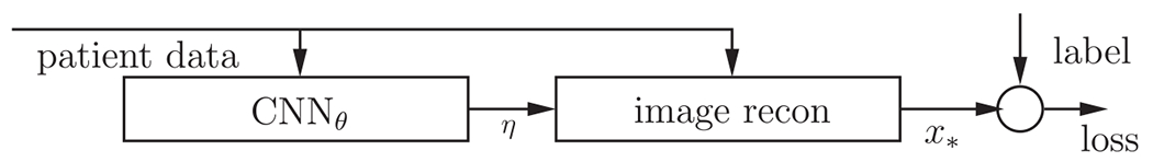
The hyperparameter learning framework proposed in (Xu and Noo 2021). The CNN, parametrized by $\theta$, generates patientspecific and spatially variant hyperparameter $\eta$ needed for optimization-based image reconstruction. End-to-end learning requires backpropagating the gradient from the loss to the CNN parameter $\theta$. During testing/inference, the image reconstruction module can run outside of a DL library.

In addition to hyperparameter learning and regularizer design, a third area where DL has entered the MBIR pipeline is data acquisition itself, i.e., to learn a system matrix.

Most works on system matrix or sampling pattern learning originated in MR and ultrasound (Milletari et al 2019), where there is more flexibility in data acquisition patterns. More recently, learning-based trajectory optimization has also emerged for advanced interventional C-arm CT systems (Zaech et al 2019). Regardless of modalities, system matrix learning faces a few common issues that affect the learning strategy:

1. Whether it is parameter-free learning or parameterized learning. Parameter-free learning (Stayman and Siewerdsen 2013, Gözcü et al 2018) often refers to the scenario where there is a finite set of candidate sampling patterns, and the task is to choose a subset in a certain optimal manner. Due to the combinatorial nature of the subset selection problem, the optimal subset is often obtained in a greedy, incremental, manner, choosing the next candidate based on the current candidates until a performance criterion is achieved, or a scan time budget is exhausted. On the other hand, it may be possible to parameterize the sampling pattern and optimize with respect to these parameters. Then continuous optimization algorithms, e.g., gradient descent, can be applied (Aggarwal and Jacob 2020).

2. What is the criterion for an optimal sampling scheme. Most approaches for sampling pattern learning include a reconstruction operator in the learning pipeline and perform supervised learning with known ground truth images. In this case, the criterion for optimality is simple: using a loss function to measure the discrepancy between the ground truth and the reconstruction. Alternatively, if a surrogate image quality measure, parameterized by the sampling pattern, is available, it is possible to directly learn to predict the surrogate measure using a regression network (Thies et al 2020).

3. Whether the clinical task requires online or offline learning. Online or active learning (Zaech et al 2019, Zhang et al 2019) aims to predict the next sampling position given the past sampling history; offline learning is to prescribe the whole sampling scheme before the acquisition starts. For some real time acquisitions, online learning may be the only option. However, if a preview or a fast scan acquiring scout views is possible, then they can be used to plan an entire trajectory before acquisition starts.

4. Whether system matrix learning is performed in isolation or in conjunction with reconstruction learning. Learning a system matrix can be performed for a fixed reconstruction algorithm, be it direct inversion, an MBIR method, or a CNN-based reconstruction module (Gözcü et al 2018). Alternatively, it is reasonable to expect that jointly optimizing the sampling pattern and the reconstruction operator can leverage the interdependency between the two and maximize performance (Aggarwal and Jacob 2020, Bahadir et al 2020).

Overall, sampling pattern or system matrix learning is still an under explored area of research. We presented some common design issues that likely transcend the boundaries of different imaging modalities. It is possible that system matrix learning finds applications in other modalities such as CT for dynamic bowtie designs (Hsieh and Pelc 2013, Huck et al 2019), or SPECT for multi-pinhole pattern optimization (Lee et al 2014), or view-based acquisition time optimization (Ghaly et al 2012, Zheng and Metzler 2012, van der Velden et al 2019).

6.2. Embedding convex optimization layers within DL pipeline

Optimization is the backbone of machine learning (ML) and deep learning (DL). At the top level, almost all DL training is based on minimizing an objective function, and applying stochastic gradient descent to obtain the network parameters. Optimization also appears at a lower level. Common DL modules such as ReLU, softmax, and sigmoid can be interpreted as nonlinear mappings where the output is the solution of a convex optimization problem (Amos 2019, chapter 2). For example, ReLU is simply the proximal mapping of the non-negativity constraint. The softmax and sigmoid are the generalized proximal mappings using the Bregman distance instead of the quadratic distance (Nesterov 2005). Active research is going on in the ML community to incorporate more generic convex optimization layers (COL) as standard modules of DL to inject domain knowledge, and to increase the modeling power and the interpretability of DL networks.

Figure 4 illustrates how a COL may be used as a module in a DL network. The input to the COL is the output of the previous layer plus additional nuisance parameters; the output of the COL layer is the solution of a convex optimization problem and serves as the input to the next layer.

Figure 4.

A convex optimization layer (COL) outputs the solution of a convex optimization problem $f(x;\theta )$, where $\theta$ lumps both the input $y$ and nuisance parameters $\eta$. A COL can be embedded as a component in a larger network. End-to-end training of such networks requires differentiation through argmin.

Applications of COL can be found in reinforcement learning (Amos et al 2018), adversarial attack planning (Biggio and Roli 2018, Agrawal et al 2019a), meta learning (Lee et al 2019), and hyperparameter learning for convex programs (Amos and Kolter 2017, Bertrand et al 2020, McCann and Ravishankar 2020). A fundamental question arising from end-to-end training of such deep networks is how to backpropagate the gradient for the COL. More specifically, the forward pass of a COL solves

$$x_{\ast }=\text{argmin}f(x;\theta )$$ (6.1)

where $f$ is a generic convex function of $x$, and $\theta$ lumps the input from the previous layer and the nuisance parameters. Given the loss function $l$ (not shown in figure 4) for training, end-to-end learning requires backpropagating the gradient at the output of the network ${\nabla }_{x_{\ast }}l$ to the network inputs ${\nabla }_{\theta }l$. In principle, such backpropagation can be obtained by applying the chain rule from elementary calculus:

$$\frac{\partial l}{\partial {\theta }_i}=\sum _j\frac{\partial x_{\ast ,j}}{\partial {\theta }_i}\frac{\partial l}{\partial x_{\ast ,j}}={\left[\frac{\partial x_{\ast }}{\partial {\theta }_i}\right]}^t{\nabla }_{x_{\ast }}l$$ (6.2)

where ${\nabla }_{\theta }l={\left[\cdots \partial l/\partial {\theta }_i\cdots \right]}^t$, and ${\left[\partial x_{\ast ,j}/\partial {\theta }_i\right]}_{\{ji\}}\equiv \partial x_{\ast }/\partial \theta$ is the Jacobian matrix. In practice, unless the problem size is small, it is more preferable to obtain ${\nabla }_{\theta }l$ directly, without an explicit matrix-vector product using the Jacobian matrix which is often infeasible.

Depending on the type of convex programs, methods for gradient calculation can be roughly grouped into four categories: (i) analytic differentiation, (ii) differentiation by unrolling, (iii) argmin differentiation using the implicit function theorem (Amos and Kolter 2017), and (iv) differentiation using fixed point iterations (Griewank and Walther 2008, Jeon et al 2021). We use the simple (unconstrained) problem (6.1) to illustrate key concepts in these methods. Very often it is more informative to specialize to a concrete example. In this case, we consider the following quadratic programming problem:

$$f(x;\theta )=\frac{1}{2}{x}^{t}Qx-b^{t}x,$$ (6.3)

where $\theta =\{Q,b\}$, and $Q\succ 0$, i.e., $Q$ is a symmetric positive definite matrix.

1. Obviously there is a closed form solution to (6.3), i.e., $x_{\ast }=Q^{-1}b$. Applying (6.2):

   $${\nabla }_{b}l={\left[\frac{\partial x_{\ast }}{\partial b}\right]}^t{\nabla }_{x_{\ast }}l=Q^{-t}{\nabla }_{x_{\ast }}l=Q^{-1}{\nabla }_{x_{\ast }}l\triangleq z$$ (6.4)

   Furthermore, applying the matrix calculus rule: $\frac{\partial Y^{-1}}{\partial t}=-Y^{-1}\frac{\partial Y}{\partial t}{Y}^{-1}$, for $t\in R$, and specializing it to a symmetric matrix,

   $$\frac{\partial l}{\partial Q_{ij}}\stackrel{(6.2)}{=}{\left[{\nabla }_{x_{\ast }}l\right]}^t\frac{\partial x_{\ast }}{\partial Q_{ij}}={\left[{\nabla }_{x_{\ast }}l\right]}^t\left(-Q^{-1}\left(\frac{\left[e_{ij}\right]+\left[e_{ji}\right]}{2}\right)Q^{-1}b\right)$$

   where $\left[e_{ij}\right]$ is a matrix of compatible dimension of all zeros except at $(i,j)$ with value 1. Arranging all elements $\partial l/\partial Q_{ij}$ into the matrix form, and recalling the definition of $z$ in (6.4), it can be verified that

   $${\nabla }_{Q}l=-Q^{-1}\frac{\left(b{\left[{\nabla }_{x_{\ast }}l\right]}^t+\left[{\nabla }_{x_{\ast }}l\right]b^t\right)}{2}{Q}^{-1}=-\frac{x_{\ast }{z}^t+z{x}_{\ast }^t}{2}$$ (6.5)

   The additional computation for the backward pass, ${\nabla }_{b}l$ and ${\nabla }_{Q}l$, amounts to solving (6.3) one more time with $b$ replaced by ${\nabla }_{x_{\ast }}$. In practice, the matrix inverse $Q^{-1}$ is not calculated; instead the matrix vector product $Q^{-1}b$ or $Q^{-1}{\nabla }_{x_{\ast }}$ is calculated by applying the conjugate gradient algorithm to (6.3). Analytic differentiation is possible if there is a closed form expression for the solution, which is unavailable for most convex optimization problems. This rather stringent requirement limits the applicability of this approach to simple problems.
2. For the generic setting (6.1), the forward pass of the COL often relies on an iterative algorithm, e.g., a gradient descent algorithm. For the specific problem (6.3), the gradient descent algorithm leads to the following update equation:

   $$x_{k+1}=x_k-\gamma \nabla f\left(x_k;\theta \right)=x_k-\gamma \left(Q{x}_k-b\right)=(I-\gamma Q)x_k+\gamma b$$ (6.6)

   where $x_k$ is the estimate of $x_{\ast }$ at $k\text{th}$ iteration, $\gamma >0$ is a step size parameter. Unrolling amounts to expand the recurrence (6.6) a fixed number of steps, for $k=0,\cdots ,K-1$, and let $x_{\ast }=x_K$. Since each step of the recursion only consists of elementary operations (similar to a fully connected layer), the backward pass can be calculated, from the last step of the recursion to the first.

   $${\nabla }_{x_k}l={(I-\gamma Q)}^t{\nabla }_{x_{k+1}}l,k=K-1,\cdots ,0.$$ (6.7a)

   $${\nabla }_{Q}l=-\gamma \sum _{i=K-1}^0\frac{\left[{\nabla }_{x_{i+1}}l\right]x_i^t+x_i{\left[{\nabla }_{x_{i+1}}l\right]}^t}{2},{\nabla }_{b}l=\gamma \sum _{i=K-1}^0{\nabla }_{x_{i+1}}l$$ (6.7b)

   It is clear that differentiation through unrolling requires storing all intermediate solutions $x_k$ in memory, which may limit the number of unrolling stages, and consequently the quality of both the forward and backward calculation.
3. Argmin differentiation in the generic setting starts with the first order optimality condition. That is, assuming $f$ is differentiable, then we have $0={\left.{\nabla }_{x}f(x;\theta )\right|}_{x_{\ast }}$. For the specific problem (6.3), this leads to

   $$0=Q{x}_{\ast }-b$$ (6.8)

   Then differentiating both sides of (6.8) with respect to the parameters gives

   $$0=dQ{x}_{\ast }+Qd{x}_{\ast }-db\stackrel{(a)}{\Rightarrow }\frac{\partial x_{\ast }}{\partial b}=Q^{-1},\left[\frac{\partial x_{\ast }}{\partial Q_{ij}}\right]=-Q^{-1}\frac{\left[e_{ij}+e_{ji}\right]}{2}{x}_{\ast }$$ (6.9)

   where in (a) of (6.9) we set $dQ=0$ and $db=0$ to derive the next two relationships, respectively. Applying the Jacobian relationship (6.2), elementary manipulation will lead to the same results as in (6.4) and (6.5). Argmin differentiation has been applied to a generic quadratic programming problem (with an objective function (6.3), and with linear equality and inequality constraints) by taking matrix differentials with respect to the KKT conditions (Amos and Kolter 2017). It has also been applied to disciplined convex programs (Agrawal et al 2019a), to cone programs (Agrawal et al 2019b), to semidefinite programs (Wang et al 2019), and other problem instances with applications in hyperparameter optimization and sparsifying-transform learning (Bertrand et al 2020, McCann and Ravishankar 2020). A weakness of argmin differentiation is that it is problem-specific: the gradient backpropagation formulas need to be derived for each class of problems.
4. Differentiation through the fixed point of an iterative algorithm has been studied in the context of automatic differentiation (or algorithmic differentiation), see, e.g., (Christianson 1994, Griewank and Walther 2008). A recent application is the so-called fixed-point iteration (FPI) layers (Jeon et al 2021) to model complex behaviors for DL applications. Unlike the previous three categories, differentiation through the fixed point can be applied to a wider class of convex problems;³¹ its implementation is also simple and can be obtained by simple adaptation of the forward computation. To illustrate the concept, we apply the gradient descent algorithm as an example of a fixed point algorithm to estimate the solution $x_{\ast }$ of (6.3). Specifically, for $k=0,\cdots$,

   $$x_{k+1}=x_k-\gamma \nabla f\left(x_k\right)=(I-\gamma Q)x_k+\gamma b$$ (6.10)

The fixed point equation of (6.10) satisfies

$$x_{\ast }=(I-\gamma Q)x_{\ast }+\gamma b$$ (6.11)

Now differentiate (6.11) with respect to b:

$$\frac{\partial x_{\ast }}{\partial b}=(I-\gamma Q)\frac{\partial x_{\ast }}{\partial b}+\gamma I\Rightarrow \frac{\partial x_{\ast }}{\partial b}=\underset{\_}{{(I-(I-\gamma Q))}^{-1}}\gamma I$$ (6.12)

Note that the underlined term directly evaluates to $(\gamma Q{)}^{-1}$. But this is only because we are working with a quadratic problem; taking this route will not help to derive a numerical algorithm for ${\nabla }_{b}l$, which is what we intend to do. So we continue without such a simplification. Combining (6.12) with the chain rule (6.2):

$${\nabla }_{b}l={\left[\frac{\partial x_{\ast }}{\partial b}\right]}^t{\nabla }_{x_{\ast }}l=\underset{\_}{\gamma {(I-(I-\gamma Q))}^{-t}{\nabla }_{x_{\ast }}l}$$ (6.13)

Denote the underlined term in (6.13) as $\bar{x}$, which satisfies a fixed point equation similar to (6.11), i.e.,

$$\overline{x}\triangleq {(I-(I-\gamma Q))}^{-t}{\nabla }_{x_{\ast }}l\iff \overline{x}=(I-\gamma Q)\overline{x}+{\nabla }_{x_{\ast }}l$$ (6.14)

The fixed point $\bar{x}$ can be obtained iteatively by

$${\overline{x}}_{k+1}=(I-\gamma Q){\overline{x}}_k+{\nabla }_{x_{\ast }}l,$$ (6.15)

which is the same gradient descent algorithm as in (6.10) with the same step size $\gamma$, but applied to ${\nabla }_{x_{\ast }}l$ instead of $\gamma$ b. Plugging (6.14) in (6.13) leads to

$${\nabla }_{b}l=\gamma \overline{x}$$ (6.16)

We can obtain ${\nabla }_{\mathrm{Q}}l$ in a similar manner, i.e., by taking derivatives with respect to the fixed point equation (6.11), which will lead to

$${\nabla }_{\text{Q}}l=-\gamma \frac{\left(x_{\ast }{\overline{x}}^t+\overline{x}{x}_{\ast }^t\right)}{2}$$ (6.17)

For the quadratic problem (6.3), differentiation through fixed point iteration amounts to (6.15), (6.16), (6.17). It is straightforward to verify that this procedure leads to the same results as in (6.4) and (6.5). In this special case, the forward pass and the backward pass are essentially identical, the convergence of the backward pass is guaranteed by the convergence of the forward pass.

For the generic problem (6.1), the backward pass can be derived by simple modifications of the forward pass (Griewank and Walther 2008, Jeon et al 2021). In terms of convergence, it was shown in (Jeon et al 2021) that if the forward pass has a gradient Lipschitz constant that is less than 1, i.e., a contraction mapping, then the backward algorithm for computing the gradient is also a contraction.

Unlike differentiation by unrolling, differentiation through fixed point iteration is of constant memory. There is no need to store the intermediate updates $x_k$, only the fixe point $x_{\ast }$ matters. In practical implementation, the fixed point iterations (FPI) for both the forward and the backward pass of the COL must be stopped at a finite iteration. The effect of finite termination, however, is unclear. Moreover, the FPI for most convex programs, e.g., gradient descent or primal-dual update (Chambolle and Pock 2021), are not contractions and may not have a unique fixed point. The applicability of differentiation through such convex programs is yet to be investigated.

The use of convex optimization layers as a module within a large DL network is still at its early stage. Its utilities to machine learning in general are still being discovered. For imaging problems, an interesting application is hyperparameter optimization for convex programs, e.g., MBIR, as we discussed in section 6.2. For this application, the combination of rigorous formulations of MBIR problems, the representation power of DL networks, and a formalism for gradient backpropagation through the convex programs for end-to-end training, is promising to remove the bottleneck of MBIR and elevate its performance.

6.3. Discussion

We show in table 2 a comparison of the different ways of combining DL and MBIR in terms of their training/testing efficiency and memory cost. This list is not exhaustive, for example, it does not include the more recent research on combining DL and MBIR in a sequential manner, where DL-produced images are subsequently refined by MBIR (Wu et al 2021a, Hayes et al 2021). Synergistic combination of DL and MBIR is picking up momentum. It is without doubt that future ingenuity will lead to more innovative network designs and/or novel synergistic use of DL and MBIR.

Table 2.

A comparison of the different embedding methods in section 6.1 and section 6.2.

	variational network	CNN-constrained image representation	COLf
training timed	***	*a	***
testing timee	+	+	+
memory	$$$b	$	$c

^aThis refers to the first variation which uses a pretrained denoising network. In the second variation there is no separate training and testing phase. Each test case requires solving a network optimization problem.

^bThe increased memory of VN is from the feature maps of the unrolled iterations.

^cBy using either argmin differentiation or differentiation through fixed-point iteration to achie ve constant memory footprint.

^dHere we use the training time of a typical denoising network as the baseline $\left({ }^{\ast }\right)$.

^eThe testing time for all three approaches is similar to that of one MBIR $(+)$.

^fHyperparameter learning can be treated as a special case of COL.

Putting the ever improving performance aside for a moment, we notice that, with very few exceptions (Yu et al 2020, Li et al 2021), commonly used performance metrics are almost exclusively simple quantitative image quality (IQ) indices such as PSNR and SSIM. Such IQ indices are easy to compute; they can be standardized to enable expedited performance evaluation with published datasets (Moen et al 2021). However, unlike natural images, medical images must be interpreted by a radiologist to make diagnosis. The simple quantitative IQ indices may not correlate with radiologists’ performance (Myers et al 1985, Barrett et al 1993), which can hinder eventual clinical translation.

Another factor hindering clinical translation is that DL networks are often unable to correctly assess their decision uncertainty (Blundell et al 2015). Such network uncertainty may arise from a lack of knowledge of the underlying data generation process or the stochastic nature of the training/testing data (Der Kiureghian and Ditlevsen 2009). This issue can be addressed by recent research efforts that provide network prediction together with network uncertainty (Gawlikowski et al 2021). For image generation (Edupuganti et al 2021, Narnhofer et al 2021, Tanno et al 2021), the uncertainty map may aid clinical decision making; furthermore, the uncertainty map can also improve the robustness of incorporating a DL-predicted prior image into MBIR (Leynes et al 2021, Wu et al 2021b).

7. Conclusions

The success of DL methods in tackling traditional computer vision tasks has earned its entrance to other fields, including medical imaging. The initial results have generated tremendous excitement over the potential of DL for solving inverse problems, leaving many to wonder if it is ‘game over’ for the more conventional MBIR.

With this question in mind, in this paper we reviewed concepts in convex optimization and first order methods, which are the backbone of many MBIR problems. We presented examples in the literature of how DL and convex optimization can work strategically together and mutually benefit each other.

As in any fast-developing field, the landscape of medical imaging is constantly changing and sudden influx of ideas creates opportunities, challenges, and even confusions. We are at a crossroads where it is ‘difficult to see; always in motion is the future.’ But we are ‘designers of our future and not mere spectators’ (Sutton and Barto 2018, chapter 17); the choices we make will determine the direction of the path that we take. Convex optimization and the reincarnated form in which it remains relevant are among the choices. We hope this paper can inject some new enthusiasm into this elegant subject.

Appendix

A.1. Bregman distance

The Bregman distance $D_h(\cdot ,\cdot )$ of (2.13) is parameterized by a differentiable function $h$, which is a $\sigma$-strongly convex function with respect to a general norm (2.3), not necessarily the 2-norm $\parallel \cdot {\parallel }_2$ induced by an inner product. Any norm, such as ${\ell }_p,p⩾1$ will do. For example, the function $h={\sum }_i{x}_i\mathrm{l}\mathrm{o}\mathrm{g}{x}_i$ that we used for calculating Bregman proximal mapping of the unit simplex, is not strongly convex in the 2-norm; it is strongly convex in the ${\ell }_1$ norm (Beck and Teboulle 2003, Nesterov 2005).

Similarly, the norm in the characterization of $L$-smooth functions ((2.1) and (2.2)) does not need to be the 2-norm. For (2.2) this requires that $⟨\cdot ,\cdot ⟩$ be interpreted as linear functionals; and for (2.1), we need to distinguish between a (primal) norm $\parallel \cdot \parallel$ and its dual norm $\parallel y{\parallel }_{\ast }:={\mathrm{s}\mathrm{u}\mathrm{p}}_x\{⟨y,x⟩,\parallel x\parallel ⩽1\}$. More specifically, (2.1) is replaced by $\parallel \nabla f\left(x\right)-\nabla f\left(y\right){\parallel }_{\ast }⩽L\parallel x-y\parallel$. With the general norm, the duality between strong convexity and (strong) $L$-smoothness still holds: a function $f$ is $L$-smooth with respect to norm $\parallel \cdot \parallel$, then its conjugate $f^{\ast }$ is $1/L$-strongly convex with respect to the dual norm $\parallel \cdot {\parallel }_{\ast }$, and vice versa, see e.g., (Juditsky and Nemirovski 2008, Kakade et al 2009). Nesterov’s accelerated gradient descent also extends to Bregman proximal gradient algorithms, as seen in algorithm 3.5. Other accelerated variants applicable to the Bregman distance can be found in (Nesterov 2005, Auslender and Teboulle 2006).

The main practical advantage of the Bregman distance is that it can be used to adapt to the problem geometry. A ‘conventional’ $L$-smooth function (defined by the 2-norm) has a global majorizer that is a quadratic function, which subsequently defines the gradient update for gradient-descent type methods. Analogously, for the general $L$-smooth function defined by the Bregman distance, the global majorizer can now be chosen to fit the problem structure, e.g., by having a smaller Lipschitz constant for a ‘custom’ distance function, which then leads to larger step sizes and faster convergence. See (Nesterov 2005), Sec 4 for an example of the effect of different norms on the Lipschitz constant.

A.2. Relative smoothness and the Poisson likelihood

A standard assumption in first order algorithms for smooth minimization is that the objective function is L-smooth, as defined by (2.2) in the convex setting or (5.2) in the nonconvex setting. This assumption is certainly satisfied by the quadratic data fitting term for most CT reconstruction problems, given in the prototype objective function (3.22). On the other hand, for SPECT and PET image reconstruction, the data fitting term is usually the negative Poisson log-likelihood, i.e., replacing the quadratic data fitting term in (3.22) by the following

$$\varphi (Ax,y)=\sum _{ij}{a}_{ij}{x}_j-\sum _i{y}_i\text{log}\sum _j{a}_{ij}{x}_j.$$ (8.1)

It is easy to verify that $\varphi$ is differentiable but its gradient is not (globally) Lipschitz continuous. As such, the simple gradient descent algorithm and any of its accelerated versions are not applicable. One approach to remedy the situation is to modify the data fitting term (8.1)—replacing Ax by Ax + r (Krol et al 2012, Zheng et al 2019), where $r>0$ is a known vector accounting for the fixed background (randoms and scatter). The modified function $\varphi (Ax+r,y)$ is $L$-smooth for $L=\parallel A{\parallel }^2{\mathrm{m}\mathrm{a}\mathrm{x}}_i\left\{y_i/r_i^2\right\}$. Other modifications for a similar purpose can be found in (Chambolle et al 2018). A potential issue for these approaches is that the gradient Lipschitz constant of the modified smooth objective may still be quite big, which affects the step size and convergence.

A notion of relative smoothness is proposed in (Bauschke et al 2017, Lu et al 2018) to lift the Lipschitz gradient requirement in first order algorithms altogether. For the (conventional) definition of $L$-smooth (2.2), an equivalent characterization is that $\frac{L}{2}\parallel x{\parallel }^2-f\left(x\right)$ is a convex function. In an analogous manner, the notion of being ‘relatively smooth’ is characterized by replacing the quadratic function by a differentiable convex function $h$, called the reference function. More precisely,

$$f(x)\text{is}L\text{-smooth relative to}h\iff Lh(\cdot )-f(\cdot )\text{is convex}$$ (8.2)

It is shown in (Lu et al 2018) that (8.2) is equivalent to

$$f(y)⩽f(x)+\langle \nabla f(x),y-x\rangle +L{D}_h(y,x),$$ (8.3)

where $D_h(y,x)=h\left(y\right)-\left[h\right(x)+⟨\nabla h(x),y-x⟩]$ is the Bregman distance (2.13), but without requiring $h$ is strongly convex in a norm. Obviously, (8.3) is a direct generalization of (2.2) by replacing the quadratic distance by $D_h(y,x)$. The notion of relatively strong convex can also be similarly defined, i.e., a function $f$ is $\mu$-strongly convex relative to $h$, if $f-\mu h$ is convex.

With the generalized definition of smoothness, the first order algorithms can be applied directly to minimization problems involving such relatively smooth functions. As a simple example, consider the composite problem of

$$\text{min }\varphi (x),\varphi (x)=f(x)+P(x)$$ (8.4)

where $f\left(x\right)$ is $L$-smooth relative to $h$, and $P$ is convex, possibly nondifferentiable. As usual, we assume $x_{\ast }=\mathrm{a}\mathrm{r}\mathrm{g}\mathrm{m}\mathrm{i}\mathrm{n}\varphi \left(x\right)$ exists. The Bregman proximal gradient descent algorithm generates $x_k$ according to

$$x_{k+1}=\text{argmin}\{P(x)+f\left(x_k\right)+\langle \nabla f\left(x_k\right),x-x_k\rangle +\frac{1}{\lambda }{D}_h\left(x,x_k\right)\},k=0,1,\cdots$$ (8.5)

It is shown in (Lu et al 2018) that, setting the step size $\lambda =1/L,\varphi \left(x_k\right)$ converges to $\varphi \left(x_{\ast }\right)$ at a rate of $𝒪(1/k)$. If $f$ is both $L$-smooth and $\mu$-strongly convex relative to $h$, then the gradient descent algorithm (8.5) exhibits linear convergence. This algorithm can also be applied to the nonconvex setting (Bolte et al 2018), where both $f$ and $P$ are nonconvex, by using a smaller step size $\lambda$.

For practical applications, the difficulty often resides in finding a reference function $h$ for the objective $f$, such that (1) $f$ is relatively smooth, i.e., to show that $Lh\left(x\right)-f\left(x\right)$ is convex for a certain $L>0$, and (2) the associated subproblem (8.5) is simple with efficient or closed form solutions. For the negative Poisson log-likelihood (8.1), it is shown in (Bauschke et al 2017) that $h\left(x\right)=-{\sum }_i\mathrm{l}\mathrm{o}\mathrm{g}{x}_i$ works, and an estimate of the Lipschitz constant is $L={\sum }_i{y}_i$. Applying (8.5) (in the absence of a nondifferentiable P), the uptake equation takes the following form:

$$\frac{1}{x_j^{k+1}}=\frac{1}{x_j^k}+\frac{{\delta }_j^k}{L},\text{where}{{\delta }_j^k\triangleq {\nabla }_x\varphi (Ax,y)|}_{x_j^k}=\sum _i{a}_{ij}-\sum _i\frac{y_i{a}_{ij}}{{\sum }_j{a}_{ij}{x}_j^k}$$

The practical convergence speed and image properties of this algorithm is unknown. Another unknown is whether minimization of relative smooth functions can enjoy the accelerated rate of $𝒪\left(1/k^2\right)$ similar to the (conventional) $L$-smooth functions by using Nesterov’s acceleration techniques.

A.3. Equivalence of a special primal-dual algorithm and the AGD

For convenience, we copy the special primal-dual algorithm (3.21) below.

$$w_{k+1}=\frac{K{\tilde{x}}_k+{\sigma }_k^{-1}{w}_k}{1+{\sigma }_k^{-1}}$$ (8.6a)

$$x_{k+1}=\text{arg min}\{g(x)+\langle Kx,\nabla h\left(w_{k+1}\right)\rangle +\frac{1}{{\tau }_k}{D}_1\left(x,x_k\right)\}$$ (8.6b)

$${\tilde{x}}_{k+1}=x_{k+1}+{\alpha }_k\left(x_{k+1}-x_k\right)$$ (8.6c)

If we choose $w_0\in \mathrm{r}\mathrm{a}\mathrm{n}\left(K\right)$, i.e., $w_0$ is in the range of $K$, then it is easy to see that $w_k\in \mathrm{r}\mathrm{a}\mathrm{n}\left(K\right)$ for all $k⩾0$. In this case, we can reparameterize $w_k$ by $w_k=K{\underset{\_}{x}}_k$; the recursion of $w_k$ can be obtained from a recursion of ${\underset{\_}{x}}_k$ as

$${\underset{\_}{x}}_{k+1}=\frac{{\tilde{x}}_k+{\sigma }_k^{-1}{\underset{\_}{x}}_k}{1+{\sigma }_k^{-1}},w_k=K{\underset{\_}{x}}_k$$ (8.7)

Combining (8.7) with (8.6b) and (8.6c), the following update equations:

$${\underset{\_}{x}}_{k+1}=\frac{{\tilde{x}}_k+{\sigma }_k^{-1}{\underset{\_}{x}}_k}{1+{\sigma }_k^{-1}}$$ (8.8a)

$$x_{k+1}=\text{argmin}\{g(x)+\langle Kx,\nabla h\left(K{\underset{\_}{x}}_{k+1}\right)\rangle +\frac{1}{{\tau }_k}{D}_1\left(x,x_k\right)\}$$ (8.8b)

$${\tilde{x}}_{k+1}=x_{k+1}+{\alpha }_k\left(x_{k+1}-x_k\right)$$ (8.8c)

will produce sequence of updates that are identical to (8.6).

Next we will show ${\underset{\_}{x}}_{k+1}$ of (8.8a) is identical to $y_k$ of algorithm 3.5. Using (8.8a) and (8.8c), we remove ${\tilde{x}}_k$ and thereby express ${\underset{\_}{x}}_k$ using $\{{\underset{\_}{x}}_k\}$ and $\left\{x_k\right\}$ only:

$${\underset{\_}{x}}_{k+1}=\frac{{\sigma }_k^{-1}{\underset{\_}{x}}_k+\left(1+{\alpha }_{k-1}\right)x_k-{\alpha }_{k-1}{x}_{k-1}}{1+{\sigma }_k^{-1}}$$ (8.9)

We now do the same for $y_k$ of algorithm 3.5. Copying step 2 and 4 of algorithm 3.5 below:

$$y_k=\left(1-{\theta }_k\right){\overline{x}}_k+{\theta }_k{x}_k$$ (8.10)

$${\overline{x}}_{k+1}=\left(1-{\theta }_k\right){\overline{x}}_k+{\theta }_k{x}_{k+1}$$ (8.11)

We will express $y_k$ using the sequence $\left\{x_k\right\}$ and $\left\{y_k\right\}$, i.e., to remove dependence on $\left\{{\bar{x}}_k\right\}$. Toward that end,

$${\overline{x}}_{k+1}\stackrel{(8.11)}{=}\left(1-{\theta }_k\right){\overline{x}}_k+{\theta }_k{x}_{k+1}\stackrel{(8.10)}{=}{y}_k-{\theta }_k{x}_k+{\theta }_k{x}_{k+1}\stackrel{(a)}{\Rightarrow }$$ (8.12a)

$${\overline{x}}_k=y_{k-1}-{\theta }_{k-1}{x}_{k-1}+{\theta }_{k-1}{x}_k$$ (8.12b)

where in (a) of (8.12a) we decrease $k$ by 1 to obtain (8.12b). Finally, we combine (8.12) and (8.11),

$${\overline{x}}_{k+1}\stackrel{(8.12a)}{=}{y}_k-{\theta }_k{x}_k+{\theta }_k{x}_{k+1}$$ (8.13a)

$$\stackrel{(8.11)}{=}\left(1-{\theta }_k\right){\overline{x}}_k+{\theta }_k{x}_{k+1}$$ (8.13b)

$$\stackrel{(8.12b)}{=}\left(1-{\theta }_k\right)\left[y_{k-1}-{\theta }_{k-1}{x}_{k-1}+{\theta }_{k-1}{x}_k\right]+{\theta }_k{x}_{k+1}$$ (8.13c)

Re-arranging the equality relationship between (8.13a) and (8.13c), then

$$y_k=\left(1-{\theta }_k\right)y_{k-1}+\left[\left(1-{\theta }_k\right){\theta }_{k-1}+{\theta }_k\right]x_k-\left(1-{\theta }_k\right){\theta }_{k-1}{x}_{k-1}$$ (8.14)

If we do a term by term matching between (8.14) and (8.9), and set the parameters according to

$${\theta }_k=\frac{1}{1+{\sigma }_k^{-1}},\text{and}\frac{{\alpha }_{k-1}}{1+{\sigma }_k^{-1}}=\left(1-{\theta }_k\right){\theta }_{k-1}\Rightarrow {\alpha }_{k-1}=\frac{\left(1-{\theta }_k\right){\theta }_{k-1}}{{\theta }_k}$$

then with compatible initializations, we have $\left\{y_k\right\}$ of algorithm 3.5 coincides with $\{{\underset{\_}{x}}_{k+1}\}$ of the special primal-dual algorithm; furthermore, by setting ${\tau }_k^{-1}={\theta }_k{L}_f$, the two sequences $\left\{x_k\right\}$ also coincides (Lan and Zhou 2018).

The convergence of $(f+g)\left({\bar{x}}_k\right)$ of algorithm 3.5 at rate $𝒪\left(1/k^2\right)$ then implies the ergodic convergence of a weighted sequence of $x_k$. More specifically, from (8.11), ${\bar{x}}_k$ is a weighted average of $x_k$ as shown below:³²

$$\begin{gathered} {\overline{x}}_k=\left(1-{\theta }_{k-1}\right){\overline{x}}_{k-1}+{\theta }_{k-1}{x}_k \\ =\left(1-{\theta }_{k-1}\right)\left[\left(1-{\theta }_{k-2}\right){\overline{x}}_{k-2}+{\theta }_{k-2}{x}_{k-1}\right]+{\theta }_{k-1}{x}_k \\ =\left(1-{\theta }_{k-1}\right)\cdots \left(1-{\theta }_1\right){\theta }_0{x}_1+\cdots +\left(1-{\theta }_{k-1}\right)\left(1-{\theta }_{k-2}\right){\theta }_{k-3}{x}_{k-2} \\ +\left(1-{\theta }_{k-1}\right){\theta }_{k-2}{x}_{k-1}+{\theta }_{k-1}{x}_k \\ \stackrel{(3.17)}{=}\frac{{\theta }_{k-1}^2}{{\theta }_{k-2}^2}\frac{{\theta }_{k-2}^2}{{\theta }_{k-3}^2}\cdots \frac{{\theta }_1^2}{{\theta }_0^2}{\theta }_0{x}_1+\cdots +\frac{{\theta }_{k-1}^2}{{\theta }_{k-3}^2}{\theta }_{k-3}{x}_{k-2}+\frac{{\theta }_{k-1}^2}{{\theta }_{k-2}^2}{\theta }_{k-2}{x}_{k-1}+{\theta }_{k-1}{x}_k \\ =\frac{{\theta }_{k-1}^2}{{\theta }_0}{x}_1+\cdots +\frac{{\theta }_{k-1}^2}{{\theta }_{k-3}}{x}_{k-2}+\frac{{\theta }_{k-1}^2}{{\theta }_{k-2}}{x}_{k-1}+\frac{{\theta }_{k-1}^2}{{\theta }_{k-1}}{x}_k \\ ={\theta }_{k-1}^2\sum _{i=1}^k{\theta }_{i-1}^{-1}{x}_i \end{gathered}$$

Furthermore,

$$\begin{gathered} {\sum }_i^k\frac{1}{{\theta }_{i-1}}=\frac{1}{{\theta }_0}+\frac{1}{{\theta }_1}+\cdots +\frac{1}{{\theta }_{k-1}} \\ \stackrel{(3.17)}{=}\frac{1}{{\theta }_0}+\left(\frac{1}{{\theta }_1^2}-\frac{1}{{\theta }_0^2}\right)\cdots +\left(\frac{1}{{\theta }_{k-2}^2}-\frac{1}{{\theta }_{k-3}^2}\right)+\left(\frac{1}{{\theta }_{k-1}^2}-\frac{1}{{\theta }_{k-2}^2}\right)=\frac{1}{{\theta }_{k-1}^2} \end{gathered}$$

In other words, ${\bar{x}}_k$ is a weighted average of $x_k$. Then convergence of ${\bar{x}}_k$ is equivalent to the ergodic convergence of the weighted $x_k$ at the same rate.

A.4. Stochastic PDHG applied to CT reconstruction

The idea is borrowed from (Lan and Zhou 2018), where it was used to draw links between PDHG and Nesterov’s AGD algorithm.

Instead of updating ${\xi }_k$ using (4.18a), consider

$${\xi }_j^{k+1}=\{\begin{array}{ll}\underset{\xi }{\text{argmax}}\{\langle y_j-A_j{x}^k,\xi \rangle -\frac{1}{2}{\Vert \xi \Vert }_{w_j^{-1}}^2-\frac{1}{2{\sigma }_j}{\Vert \xi -{\xi }_j^k\Vert }_{w_j^{-1}}^2\}\hfill & j=j_k\hfill \\ {\xi }_j^k\hfill & j\ne j_k\hfill \end{array}$$ (8.15)

where the only change is that we use in (8.15) a weighted quadratic distance, with matching weighting coefficients as in the conjugate function $\frac{1}{2}\parallel \xi {\parallel }_{w_j^{-1}}^2$.

Let $j=j_k$. Taking derivative with respect to ${\xi }_j$

$$0\triangleq y_j-A_j{x}^k-w_j^{-1}\xi -{\sigma }_j^{-1}{w}_j^{-1}\left(\xi -{\xi }_j^k\right)\Rightarrow {\xi }_j^{k+1}=\frac{w_j\left(y_j-A_j{x}^k\right)+{\sigma }_j^{-1}\cdot {\xi }_j^k}{1+{\sigma }_j^{-1}}$$ (8.16)

Now we make change variables so that ${\xi }_k$ update can be performed equivalently in the primal domain. Define ${\tilde{v}}_j^k=-A_j^t{\xi }_j^k$, from (8.16), if $j=j_k$,

$${\tilde{v}}_j^{k+1}=-A_j^t{\xi }_j^{k+1}=\frac{-A_j^t{w}_j\left(y_j-A_j{x}^k\right)-{\sigma }_j^{-1}{A}_j^t{\xi }_j^k}{1+{\sigma }_j^{-1}}=\frac{\nabla F_j\left(x^k\right)+{\sigma }_j^{-1}{\tilde{v}}_j^k}{1+{\sigma }_j^{-1}}$$ (8.17)

where the last equality is due to the definition of the data fitting term $F_j\left(x\right)=\frac{1}{2}{∥y_j-A_{j}x∥}_{w_j}^2$. This update equation leads to algorithm 4.4.

A.5. The proximal mapping of the log prior

The proximal mapping of a nonconvex function involves a nonconvex optimization problem; care should be taken to distinguish between the local and global minimizers. The $\mathrm{l}\mathrm{o}\mathrm{g}$ prior, $f_{\mu }\left(x\right)=\mathrm{l}\mathrm{o}\mathrm{g}(1+|x|/\mu ),x\in R$, is often used in imaging applications (Mehranian et al 2013, Zeng et al 2017); we use it as an example to illustrate some typical issues associated with nonconvexity. The problem is given as the following:

$${\text{prox}}_{\left(\tau f_{\mu }\right)}(\tilde{x})=\arg \underset{x}{\min }\{f_{\mu }(x)+\frac{1}{2\tau }{\left|\tilde{x}-x\right|}^2\}\text{where}{f}_{\mu }(x)=\text{log}\left(1+\frac{\left|x\right|}{\mu }\right)$$ (8.18)

Note that the log prior has a difference-of-convex decomposition. Indeed,

$$\text{log}\left(1+\frac{\left|x\right|}{\mu }\right)=\frac{\left|x\right|}{\mu }-\frac{1}{\mu }\left(|x|-\mu \text{log}\left(1+\frac{|x|}{\mu }\right)\right)$$

from which we recognize the term in the parentheses is just the Fair potential. From our discussion in section 5.1, the $\mathrm{l}\mathrm{o}\mathrm{g}$ prior is $1/{\mu }^2$ - weakly convex, as the Fair potential itself is $1/\mu$-smooth.

It is straightforward to see that ${\mathrm{p}\mathrm{r}\mathrm{o}\mathrm{x}}_{\left(\tau f_{\mu }\right)}\left(\tilde{x}\right)$ in (8.18) is an odd function, i.e., ${\mathrm{p}\mathrm{r}\mathrm{o}\mathrm{x}}_{\left(\tau f_{\mu }\right)}(-|\tilde{x}\left|\right)=-{\mathrm{p}\mathrm{r}\mathrm{o}\mathrm{x}}_{\left(\tau f_{\mu }\right)}\left(\right|\tilde{x}\left|\right)$. Furthermore, it can be shown that ${\mathrm{p}\mathrm{r}\mathrm{o}\mathrm{x}}_{\left(\tau f_{\mu }\right)}\left(\tilde{x}\right)=\mu {\mathrm{p}\mathrm{r}\mathrm{o}\mathrm{x}}_{\left(\left(\tau /{\mu }^2\right)f_1\right)}(\tilde{x}/\mu )$. Therefore it suffices to consider the following ‘normalized’ version of (8.18):

$$\begin{gathered} \text{min }\varphi (x)\triangleq f(x)+q(x), \\ f(x)=\text{log}(1+x),q(x)=\frac{1}{2\tau }{\left|\tilde{x}-x\right|}^2,\text{where}\tilde{x}⩾0,\to \text{argmin}\triangleq x_{\ast } \end{gathered}$$ (8.19)

Our characterization of the solution to (8.19) relies on studying the gradients of the component functions $f^{\prime }\left(x\right)=1/(1+x)$ and $q^{\prime }\left(x\right)=(x-\tilde{x})/\tau$ in a graphical manner, which makes the distinction between the local and the global minima both transparent and intuitive. The developed intuition should help similar derivations for the proximal mapping of other nonconvex functions.

We plot both $f^{\prime }\left(x\right)$ and (the negated gradient) $-q^{\prime }\left(x\right)$, for $x>0$, in one graph as shown in figure 5. The gradient $-q^{\prime }\left(x\right)$ intersects the $x$-axis at $\tilde{x}$. When $\tilde{x}>0$ increases, the green line $-q^{\prime }\left(x\right)$ translates to the right. The intersection(s) between $f^{\prime }\left(x\right)$ (the blue curve) and $-q^{\prime }\left(x\right)$ (the green line) satisfy the first order optimality condition; they are the stationary points and candidate solutions $x_{\ast }$. Moreover, for any $\tilde{x}⩾0$, the solution $x_{\ast }$ to (8.19) is non-negative; the boundary of the eligible region $x=0$ requires special consideration.

Figure 5 shows the solution when $\tau ⩽1$. In this case, $-q^{\prime }\left(x\right)$ is ‘more vertical’ than any parts of $f^{\prime }\left(x\right)$. When $\tilde{x}<\tau$ (figure 5(a)), there is no intersection between $f^{\prime }\left(x\right)$ and $-q^{\prime }\left(x\right)$ within the eligible region $x⩾0$. That is, the first order optimality condition does not hold for any $x⩾0$. On the other hand, since $f^{\prime }\left(x\right)⩾-q^{\prime }\left(x\right)$, the objective $\varphi \left(x\right)$ is continuously increasing. There is a unique global minimizer at $x=0$. When $\tilde{x}>\tau$ (figure 5(b)), the green line $-q^{\prime }\left(x\right)$ translates further to the right. There is always a unique intersection between $f^{\prime }\left(x\right)$ and $-q^{\prime }\left(x\right)$, marked by the filled red marker $x_{\text{., }}$ which leads to the solution $x_{\ast }=x_{\text{.}}$. Note that when $\tau ⩽1$ the objective $\varphi$ in (8.19) is strictly convex. The solution $x_{\ast }$ depends continuously on the input $\tilde{x}$, which can be verified from figure 5.

When $\tau >1$ (figure 6 and 7), the green line $-q^{\prime }\left(x\right)$ is ‘more horizontal’ than before, the intersections between $f^{\prime }\left(x\right)$ and $-q^{\prime }\left(x\right)$ become more complicated. Figure 6 shows what happens for two extreme values of $\tilde{x}$. If $\tilde{x}>\tau$ (figure 6(a)), there is again one unique intersection between $-q^{\prime }\left(x\right)$ and $f^{\prime }\left(x\right)$, indicated by the filled red marker x. As $f^{\prime }\left(x\right)⩽-q^{\prime }\left(x\right)$ for $0⩽x⩽x$., the objective $\varphi \left(x\right)$ is continuously decreasing. Therefore this intersection $x$. is indeed the global minimizer $x_{\ast }$.

As $\tilde{x}$ decreases from $\tau$, we notice (figure 6(b)) that there is a critical value ${\tilde{x}}_t$ such that when $\tilde{x}={\tilde{x}}_t,f^{\prime }\left(x\right)$ is tangent to $-q^{\prime }\left(x\right)$; this coincidence is depicted as the dotted cyan line in figure 6(b). When $\tilde{x}<{\tilde{x}}_t$, there is no intersection between $f^{\prime }\left(x\right)$ and $-q^{\prime }\left(x\right)$. Similar to figure 5(a), since $f^{\prime }\left(x\right)>-q^{\prime }\left(x\right)$ holds for all $x⩾0$, the function $\varphi \left(x\right)$ is continuously increasing for $x⩾0$, therefore $x_{\ast }=0$ is the global minimizer.

More complications arise when ${\tilde{x}}_t⩽\tilde{x}⩽\tau$ as shown in figure 7. There are two intersections between $f^{\prime }\left(x\right)$ and $-q^{\prime }\left(x\right)$, indicated by the open $x_{\circ }$ and filled $x_{\text{. }}$ red markers. We consider the two subcases shown in (a) and (b), which have different areas in the two shaded regions, area $\mathrm{A}\lessgtr$ area $\mathrm{B}$, When $\tilde{x}$ is slightly exceeding ${\tilde{x}}_t$ (figure 7(a)), area $\mathrm{A}>$ area $\mathrm{B}$; we claim that the $x_{\circ }$ is a local maximum, and x. is a local minimum, and the global minimizer is at $x_{\ast }=0$. The reasoning is simple. When $x<x_{\circ }{f}^{\prime }\left(x\right)⩾-g^{\prime }\left(x\right)$, so the objective $\varphi \left(x\right)$ increases; when $x_{\circ }<x⩽x_{\circ },f^{\prime }\left(x\right)⩽-g^{\prime }\left(x\right)$, so the objective $\varphi \left(x\right)$ decreases. As the total amount of function value increase or decrease is exactly the area of the shaded regions, by our assumption that area $\mathrm{A}>$ area $\mathrm{B}$, the function value increase is larger than the function value decrease. Therefore, $\varphi \left(0\right)<\varphi \left(x_{\mathrm{•}}\right)<\varphi \left(x_{\circ }\right),x_{\ast }=0$ is the global minimal, $x_{\circ }$ is a local maximum, and x. is a local minimum. Similar analysis for the situation in figure 7(b) will lead to the claim that, when area $\mathrm{A}<$ area $\mathrm{B},\varphi \left(x_{\mathrm{•}}\right)<\varphi \left(0\right)<\varphi \left(x_{\circ }\right),x=0$ is a local minimal, $x_{\circ }$ is a local maximum, and $x_{\ast }=x$. is the global minimal.

The solution to (8.19), see figure 8 for an illustration, can be summarized as the following

$$x_{\ast }=\{\begin{array}{ll}0\hfill & \tilde{x}⩽{\tilde{x}}_c\hfill \\ x.\hfill & \tilde{x}>{\tilde{x}}_c\hfill \end{array}$$ (8.20)

where $x$. satisfies the first order optimality condition for (8.19):

$$0=\frac{1}{1+x_{\cdot }}+\frac{x_{\cdot }-\tilde{x}}{\tau }$$ (8.21)

When there is more than one solutions to (8.21), $x$. should take the larger value. The cutoff (threshold) of (8.20) is ${\tilde{x}}_c=\tau$ if $\tau ⩽1$. When $\tau >1,{\tilde{x}}_c$ can be calculated from the following coupled $\left({\tilde{x}}_c,x^{\prime }\right)$ equations:

$$\frac{1}{2\tau }{\left|{\tilde{x}}_c\right|}^2=\text{log}\left(1+x^{\prime }\right)+\frac{1}{2\tau }{\left|{\tilde{x}}_c-x^{\prime }\right|}^2$$ (8.22a)

$$0=\frac{1}{1+x^{\prime }}+\frac{x^{\prime }-{\tilde{x}}_c}{\tau }$$ (8.22b)

where (8.22a) is equivalent to the equal area criterion in figure 7, i.e., $\varphi \left(0\right)=\varphi \left(x^{\prime }\right)$, and (8.22b) simply expresses the intersection between $f^{\prime }\left(x\right)$ and $-q^{\prime }\left(x\right)$ at $x^{\prime }$. The closed-form solution to (8.22) is inaccessible. Instead of using the thresholding form (8.20), in practice the global minimizer is often determined by evaluating the objective $\varphi$ at the two possible candidates $x=0$ and $x=x$., see, e.g., (Gong et al 2013). Note that when $\tilde{x}={\tilde{x}}_c$, $\varphi \left(0\right)=\varphi \left(x^{\prime }\right)$, and both 0 and $x^{\prime }$ are global minima. As $\tilde{x}$ approaches to ${\tilde{x}}_c$ from left and right, there is a jump in the solution $x_{\ast }$ from 0 to $x^{\prime }$ which is strictly positive (figure 8(b)). This discontinuous behavior with respect to the data is also well-known for nonconvex optimization.

Figure 5.

(a) When $\tau ⩽1$ and $\tilde{x}⩽\tau$, the objective $\varphi$ continuously increases as a function of $x$. There is a global minimizer at $x=0$. (b) When $\tau ⩽1$ and $\tilde{x}>\tau$ there is a unique intersection point (the filled red marker) between the two gradient lines $f^{\prime }\left(x\right)$ and $-q^{\prime }\left(x\right)$.

Figure 6.

(a) If $\tau >1$ and $\tilde{x}>\tau$, there is a unique intersection between $f^{\prime }\left(x\right)$ (blue curve) and $-q^{\prime }\left(x\right)$ (green line), indicated by the filled red marker. (b) If $\tau >1$ and $\tilde{x}<{\tilde{x}}_t$, there is no intersection between the $f^{\prime }\left(x\right)$ and $-q^{\prime }\left(x\right)$. The solution to (8.19) is $x=0$. Here $x_t=\sqrt{\tau }-1,{\tilde{x}}_t=2\sqrt{\tau }-1$.

Figure 7.

Two cases when ${\tilde{x}}_t<\tilde{x}⩽\tau$. The intersections between the blue curve $f^{\prime }\left(x\right)$ and the green line $-q^{\prime }\left(x\right)$ are marked by the open and the filled red markers. The former indicates a local maximum, the latter indicates a local minimum. There is another local minimum at $x=0$. (a) When area $\mathrm{A}>$ area $\mathrm{B}$, the global minimizer of (8.19) is at $x_{\ast }=0$. (b) When area $\mathrm{A}<$ area $\mathrm{B}$, the global minimizer is at $x_{\ast }=x_{\text{. }}$, the second (larger) intersection point. The critical point $\tilde{x}={\tilde{x}}_c$ separating the two cases is when area $\mathrm{A}=$ area $\mathrm{B}$.

Figure 8.

The thresholding solution given by (8.20). Here we append by symmetry the solution for $\tilde{x}<0$ as well. (a) If $\tau ⩽1$, the objective (8.19) is convex, the solution $x_{\ast }$ is a continuous function of $\tilde{x}$. (b) If $\tau >1$, the objective (8.19) is nonconvex, the solution $x_{\ast }$ has a jump at $\tilde{x}={\tilde{x}}_c$, given by (8.22).

References

- Abdalah M, Mitra D, Boutchko R and Gullberg GT 2013. Optimization of regularization parameter in a reconstruction algorithm 2013 IEEE Nuclear Science Symposium and Medical Imaging Conference (Seoul, Korea South, 27 October–2 November 2013) (Picastaway, NJ: IEEE; ) pp 1–4 [Google Scholar]
- Adler J and Öktem O 2018. Learned primal-dual reconstruction IEEE Trans. Med. Imaging 37 1322–32 [DOI] [PubMed] [Google Scholar]
- Agrawal A, Amos B, Barratt S, Boyd S, Diamond S and Kolter Z 2019a. Differentiable convex optimization layers Proceedings of 2019 Advances in Neural Information Processing Systems 32 pp 9562–74 arXiv:1910.12430 [Google Scholar]
- Agrawal A, Barratt S, Boyd S, Busseti E and Moursi WM 2019b. Differentiating through a cone program Journal of Applied and Numerical Optimization 1 107–15 (http://jano.biemdas.com/archives/931) [Google Scholar]
- Aggarwal HK and Jacob M 2020. J-MoDL: joint model-based deep learning for optimized sampling and reconstruction, IEEE Journal of Selected Topics in Signal Processing 14 1151–62 [DOI] [PMC free article] [PubMed] [Google Scholar]
- Ahn M, Pang J-S and Xin J 2017. Difference-of-convex learning: directional stationarity, optimality, and sparsity SIAM J. Optim 27 1637–65 [Google Scholar]
- Alacaoglu A, Fercoq O and Cevher V 2019. On the convergence of stochastic primal-dual hybrid gradient arXiv:1911.00799 [Google Scholar]
- Allen-Zhu Z 2017. Katyusha: The first direct acceleration of stochastic gradient methods The Journal of Machine Learning Research 18 8194–244 [Google Scholar]
- Allen-Zhu Z and Hazan E 2016. Optimal black-box reductions between optimization objectives arXiv: 1603.05642 [Google Scholar]
- Allen-Zhu Z and Yuan Y 2016. Improved svrg for non-strongly-convex or sum-of-non-convex objectives International Conference on Machine Learning pp 1080–9 PMLR [Google Scholar]
- Amos B. Differentiable optimization-based modeling for machine learning. Carnegie Mellon University; 2019. PhD Thesis. [Google Scholar]
- Amos B, Jimenez I, Sacks J, Boots B and Kolter JZ 2018. Differentiable MPC for end-to-end planning and control Advances in Neural Information Processing Systems 31 8289–300 [Google Scholar]
- Amos B and Kolter JZ 2017. Optnet: differentiable optimization as a layer in neural networks International Conference on Machine Learning pp 136–45 PMLR [Google Scholar]
- Antun V, Renna F, Poon C, Adcock B and Hansen AC 2020. On instabilities of deep learning in image reconstruction and the potential costs of AI Proc. Natl Acad. Sci 117 30088–95 [DOI] [PMC free article] [PubMed] [Google Scholar]
- Attouch H and Bolte J 2009. On the convergence of the proximal algorithm for nonsmooth functions involving analytic features Math. Program 116 5–16 [Google Scholar]
- Attouch H, Bolte J and Svaiter BF 2013. Convergence of descent methods for semi-algebraic and tame problems: proximal algorithms, forward-backward splitting, and regularized gauss-seidel methods Math. Program 137 91–129 [Google Scholar]
- Attouch H, Bolte J, Redont P and Soubeyran A 2010. Proximal alternating minimization and projection methods for nonconvex problems: an approach based on the kurdyka-łojasiewicz inequality Math. Oper. Res 35 438–57 [Google Scholar]
- Auslender A and Teboulle M 2006. Interior gradient and proximal methods for convex and conic optimization SIAM J. Optim 16 697–725 [Google Scholar]
- Bačák M and Borwein JM 2011. On difference convexity of locally Lipschitz functions, Optimization 60 961–78 [Google Scholar]
- Bahadir CD, Wang AQ, Dalca AV and Sabuncu MR 2020. Deep-learning-based optimization of the under-sampling pattern in MRI, IEEE Transactions on Computational Imaging 6 1139–52 [Google Scholar]
- Banert S and Bot RI 2019. A general double-proximal gradient algorithm for DC programming Math. Program 178 301–26 [DOI] [PMC free article] [PubMed] [Google Scholar]
- Bao P et al. 2019. Convolutional sparse coding for compressed sensing CT reconstruction, IEEE Trans. Med. Imaging 38 2607–19 [DOI] [PubMed] [Google Scholar]
- Barrett HH, Yao J, Rolland JP and Myers KJ 1993. Model observers for assessment of image quality Proc. Natl Acad. Sci 90 9758–65 [DOI] [PMC free article] [PubMed] [Google Scholar]
- Bauschke HH, Bolte J and Teboulle M 2017. A descent lemma beyond Lipschitz gradient continuity: first-order methods revisited and applications Math. Oper. Res 42 330–48 [Google Scholar]
- Bauschke Heinz H and Borwein Jonathan M 1997. Legendre Functions and the Method of Random Bregman Projections Journal of Convex Analysis 4 27–47 [Google Scholar]
- Bauschke HH et al. 2011. Convex analysis and monotone operator theory in Hilbert spaces 408 (Berlin: Springer; ) [Google Scholar]
- Beck A 2017. First-Order Methods in Optimization (Philadelphia, PA: Society for Industrial and Applied Mathematics; ) [Google Scholar]
- Beck A and Teboulle M 2003. Mirror descent and nonlinear projected subgradient methods for convex optimization Oper. Res. Lett 31 167–75 [Google Scholar]
- Beck A and Teboulle M 2009. A fast iterative shrinkage-thresholding algorithm for linear inverse problems, SIAM J. Imag. Sci 2 183–202 [Google Scholar]
- Bertrand Q, Klopfenstein Q, Blondel M, Vaiter S, Gramfort A and Salmon J 2020. Implicit differentiation of Lasso-type models for hyperparameter optimization International Conference on Machine Learning pp 810–21 PMLR [Google Scholar]
- Bertsekas D 1999. Nonlinear Programming (Belmont, Mass: Athena Scientific; ) [Google Scholar]
- Biggio B and Roli F 2018. Wild patterns: ten years after the rise of adversarial machine learning Pattern Recognit. 84 317–31 [Google Scholar]
- Blundell C, Cornebise J, Kavukcuoglu K and Wierstra D 2015. Weight uncertainty in neural network International Conference on Machine Learning pp 1613–22 PMLR [Google Scholar]
- Bohm A and Wright SJ 2021. Variable smoothing for weakly convex composite functions J. Optim. Theory Appl 188 628–49 [DOI] [PMC free article] [PubMed] [Google Scholar]
- Bolte J, Sabach S and Teboulle M 2014. Proximal alternating linearized minimization for nonconvex and nonsmooth problems Math. Program 146 459–94 [Google Scholar]
- Bolte J, Sabach S, Teboulle M and Vaisbourd Y 2018. First order methods beyond convexity and Lipschitz gradient continuity with applications to quadratic inverse problems SIAM J. Optim 28 2131–51 [Google Scholar]
- Bot RI, Csetnek ER and Nguyen D-K 2019. A proximal minimization algorithm for structured nonconvex and nonsmooth problems SIAM J. Optim 29 1300–28 [Google Scholar]
- Bottou L, Curtis FE and Nocedal J 2018. Optimization methods for large-scale machine learning SIAM Rev. 60 223–311 [Google Scholar]
- Boyd SP and Vandenberghe L 2004. Convex Optimization (Cambridge, UK: Cambridge University Press; ) [Google Scholar]
- Bredies K, Kunisch K and Pock T 2010. Total generalized variation SIAM J. Imag. Sci 3 492–526 [Google Scholar]
- Bregman LM 1967. The relaxation method of finding the common point of convex sets and its application to the solution of problems in convex programming USSR computational mathematics and mathematical physics 7 200–17 [Google Scholar]
- Bubeck S 2015. Convex optimization: Algorithms and complexity Foundations and Trends® in Machine Learning 8 231–357 [Google Scholar]
- Candes EJ, Wakin MB and Boyd SP 2008. Enhancing sparsity by reweighted l1 minimization Journal of Fourier analysis and applications 14 877–905 [Google Scholar]
- Censor Y and Lent A 1981. An lterative Row-Action Method for Interval Convex Programming Journal of Optimization Theory and Applications 34 321–53 [Google Scholar]
- Censor Y, Herman GT and Jiang M 2017. Special issue on superiorization: theory and applications Inverse Prob. 33 040301–E2 [Google Scholar]
- Censor Y and Zenios SA 1992. Proximal Minimization Algorithm with D-Functions Journal of Optimization Theory and Applications 73 451–64 [Google Scholar]
- Cevher V, Becker S and Schmidt M 2014. Convex optimization for big data: Scalable, randomized, and parallel algorithms for big data analytics IEEE Signal Process Mag. 31 32–43 [Google Scholar]
- Chambolle A and Dossal C 2015. On the convergence of the iterates of the ”fast iterative shrinkage/thresholding algorithm J. Optim. Theory Appl 166 968–82 [Google Scholar]
- Chambolle A, Ehrhardt MJ, Richtárik P and Schonlieb C-B 2018. Stochastic primal-dual hybrid gradient algorithm with arbitrary sampling and imaging applications SIAM J. Optim 28 2783–808 [Google Scholar]
- Chambolle A and Lions P-L 1997. Image recovery via total variation minimization and related problems Numer. Math 76 167–88 [Google Scholar]
- Chambolle A and Pock T 2011. A first-order primal-dual algorithm for convex problems with applications to imaging J. Math. Imaging Vis 40 120–45 [Google Scholar]
- Chambolle A and Pock T 2016. An introduction to continuous optimization for imaging, Acta Numerica 25 161–319 [Google Scholar]
- Chambolle A and Pock T 2016. On the ergodic convergence rates of a first-order primal-dual algorithm Math. Program 159 253–87 [Google Scholar]
- Chambolle A and Pock T 2021. Learning consistent discretizations of the total variation SIAM J. Imag. Sci 14 778–813 [Google Scholar]
- Chen C, He B, Ye Y and Yuan X 2016. The direct extension of ADMM for multi-block convex minimization problems is not necessarily convergent Math. Program 155 57–79 [Google Scholar]
- Chen L, Sun D and Toh K-C 2017. A note on the convergence of ADMM for linearly constrained convex optimization problems Comput. Optim. Appl 66 327–43 [Google Scholar]
- Chen P, Huang J and Zhang X 2013. A primal-dual fixed point algorithm for convex separable minimization with applications to image restoration Inverse Prob. 29 025011 [Google Scholar]
- Chen P, Huang J and Zhang X 2016. A primal-dual fixed point algorithm for minimization of the sum of three convex separable functions, Fixed Point Theory and Applications 2016 1–18 [Google Scholar]
- Chen Y, Lan G and Ouyang Y 2014. Optimal primal-dual methods for a class of saddle point problems SIAM J. Optim 24 1779–814 [Google Scholar]
- Chen Y, Ranftl R and Pock T 2014. Insights into analysis operator learning: from patch-based sparse models to higher order MRFs IEEE Trans. Image Process 23 1060–72 [DOI] [PubMed] [Google Scholar]
- Christianson B 1994. Reverse accumulation and attractive fixed points Optimization Methods and Software 3 311–26 [Google Scholar]
- Combettes PL and Pesquet J-C 2011. Proximal splitting methods in signal processing Fixed-Point Algorithms for Inverse Problems in Science and Engineering (Berlin: Springer; ) pp 185–212 [Google Scholar]
- Condat L 2013. A primal-dual splitting method for convex optimization involving Lipschitzian, proximable and linear composite terms J. Optim. Theory Appl 158 460–79 [Google Scholar]
- Condat L, Malinovsky G and Richtárik P 2020. Distributed proximal splitting algorithms with rates and acceleration online arXiv 1 1–27 arXiv:2010.00952 [Google Scholar]
- Corda-D’ncan G, Schnabel JA and Reader AJ 2021. Memory-efficient training for fully unrolled deep learned PET image reconstruction with iteration-dependent targets IEEE Transactions on Radiation and Plasma Medical Sciences Online early access 1 1–1 [DOI] [PMC free article] [PubMed] [Google Scholar]
- Dang C and Lan G 2014. Randomized first-order methods for saddle point optimization arXiv:1409.8625 [Google Scholar]
- Davis D and Yin W 2017. A three-operator splitting scheme and its optimization applications, Set-valued and variational analysis 25 829–58 [Google Scholar]
- Defazio A, Bach F and Lacoste-Julien S 2014. SAGA: a fast incremental gradient method with support for non-strongly convex composite objectives arXiv:1407.0202 [Google Scholar]
- Dekel O, Gilad-Bachrach R, Shamir O and Xiao L 2012. Optimal distributed online prediction using mini-batches Journal of Machine Learning Research 13 165–202 [Google Scholar]
- Devolder O, Glineur F and Nesterov Y 2012. Double smoothing technique for large-scale linearly constrained convex optimization SIAM J. Optim 22 702–27 [Google Scholar]
- Devolder O, Glineur F and Nesterov Y 2014. First-order methods of smooth convex optimization with inexact oracle Math. Program 146 37–75 [Google Scholar]
- de Oliveira W 2020. The abc of dc programming Set-Valued and Variational Analysis 28 679–706 [Google Scholar]
- Der Kiureghian A and Ditlevsen O 2009. Aleatory or epistemic? does it matter? Struct. Saf 31 105–12 [Google Scholar]
- Driggs D, Ehrhardt MJ and Schönlieb C-B 2020. Accelerating variance-reduced stochastic gradient methods Math. Program 0 1–45 [Google Scholar]
- Drori Y, Sabach S and Teboulle M 2015. A simple algorithm for a class of nonsmooth convex-concave saddle-point problems Oper. Res. Lett 43209–14 [Google Scholar]
- Duchi JC, Shalev-Shwartz S, Singer Y and Tewari A 2010. Composite objective mirror descent COLT 2010 - The 23rd Conference on Learning Theory (Haifa, Israel) pp14–26 [Google Scholar]
- Duncan JS, Insana MF and Ayache N 2019. Biomedical imaging and analysis in the age of big data and deep learning [scanning the issue] Proc. IEEE 108 3–10 [Google Scholar]
- Edupuganti V, Mardani M, Vasanawala S and Pauly J 2021. Uncertainty quantification in deep MRI reconstruction IEEE Trans. Med. Imaging 40239–50 [DOI] [PMC free article] [PubMed] [Google Scholar]
- Francisco Facchinei and Jong-Shi Pang 2003. Finite-Dimensional Variational Inequalities and Complementarity Problems (Springer Series in Operations Research) II (New York, NY: Springer-Verlag; ) [Google Scholar]
- Fan J and Li R 2001. Variable selection via nonconcave penalized likelihood and its oracle properties J. Am. Stat. Assoc 961348–60 [Google Scholar]
- Fang C, Li CJ, Lin Z and Zhang T 2018. Spider: near-optimal non-convex optimization via stochastic path integrated differential estimator arXiv:1807.01695 [Google Scholar]
- Fukushima M and Mine H 1981. A generalized proximal point algorithm for certain non-convex minimization problems Int. J. Syst. Sci 12 989–1000 [Google Scholar]
- Gawlikowski J. A survey of uncertainty in deep neural networks arXiv:2107.03342. 2021.
- Ghaly M, Links J, Du Y and Frey E 2012. Optimization of SPECT using variable acquisition duration J. Nucl. Med 53 2411–2411 [Google Scholar]
- Ghani MU and Karl WC 2018. Deep learning based sinogram correction for metal artifact reduction Electron. Imaging 2018 472 [Google Scholar]
- Gong K, Catana C, Qi J and Li Q 2018b. PET image reconstruction using deep image prior IEEE Trans. Med. Imaging 38 1655–65 [DOI] [PMC free article] [PubMed] [Google Scholar]
- Gong K, Guan J, Kim K, Zhang X, Yang J, Seo Y, El Fakhri G, Qi J and Li Q 2018a. Iterative PET image reconstruction using convolutional neural network representation IEEE Trans. Med. Imaging 38 675–85 [DOI] [PMC free article] [PubMed] [Google Scholar]
- Gong P, Zhang C, Lu Z, Huang J and Ye J 2013. A general iterative shrinkage and thresholding algorithm for non-convex regularized optimization problems, International Conference on Machine Learning 37–45 [PMC free article] [PubMed] [Google Scholar]
- Gotoh J-y, Takeda A and Tono K 2018. DC formulations and algorithms for sparse optimization problems Math. Program 169 141–76 [Google Scholar]
- Gözcü B, Mahabadi RK, Li Y-H, Ilıcak E, Cukur T, Scarlett J and Cevher V 2018. Learning-based compressive MRI IEEE Trans. Med. Imaging 37 1394–406 [DOI] [PubMed] [Google Scholar]
- Greenspan H, Van Ginneken B and Summers RM 2016. Guest editorial deep learning in medical imaging: Overview and future promise of an exciting new technique IEEE Trans. Med. Imaging 35 1153–9 [Google Scholar]
- Griewank A and Walther A 2008. Evaluating Derivatives: principles and techniques of algorithmic differentiation (Other Titles in Applied Mathematics) 2nd edn (Philadelphia, PA: SIAM; ) ( 10.1137/1.9780898717761) [DOI] [Google Scholar]
- Guo K, Han D and Wu T-T 2017. Convergence of alternating direction method for minimizing sum of two nonconvex functions with linear constraints Int. J. Comput. Math 94 1653–69 [Google Scholar]
- Gupta H, Jin KH, Nguyen HQ, McCann MT and Unser M 2018. CNN-based projected gradient descent for consistent CT image reconstruction IEEE Trans. Med. Imaging 37 1440–53 [DOI] [PubMed] [Google Scholar]
- Häggström I, Schmidtlein CR, Campanella G and Fuchs TJ 2019. DeepPET: a deep encoder-decoder network for directly solving the PET image reconstruction inverse problem Med. Image Anal 54 253–62 [DOI] [PMC free article] [PubMed] [Google Scholar]
- Hammernik K, Klatzer T, Kobler E, Recht MP, Sodickson DK, Pock T and Knoll F 2018. Learning a variational network for reconstruction of accelerated MRI data Magn. Reson. Med 79 3055–71 [DOI] [PMC free article] [PubMed] [Google Scholar]
- Hartman P et al. 1959. On functions representable as a difference of convex functions Pacific Journal of Mathematics 9 707–13 [Google Scholar]
- Hayes JW, Montoya J, Budde A, Zhang C, Li Y, Lia K, Hsieh J and Chen G-H 2021. High pitch helical CT reconstruction IEEE Trans. Med. Imaging 40 pp 3077–3088 [DOI] [PubMed] [Google Scholar]
- Herman GT, Garduño E, Davidi R and Censor Y 2012. Superiorization: an optimization heuristic for medical physics Med. Phys 39 5532–46 [DOI] [PubMed] [Google Scholar]
- Holt KM 2014. Total nuclear variation and Jacobian extensions of total variation for vector fields IEEE Trans. Image Process 23 3975–89 [DOI] [PubMed] [Google Scholar]
- Hong M, Luo Z-Q and Razaviyayn M 2016. Convergence analysis of alternating direction method of multipliers for a family of nonconvex problems SIAM J. Optim 26 337–64 [Google Scholar]
- Hsieh SS and Pelc NJ 2013. The feasibility of a piecewise-linear dynamic bowtie filter Med. Phys 40 031910–1 [DOI] [PMC free article] [PubMed] [Google Scholar]
- Huck SM, Fung GS, Parodi K and Stierstorfer K 2019. Sheet-based dynamic beam attenuator-a novel concept for dynamic fluence field modulation in x-ray CT Med. Phys 46 5528–37 [DOI] [PubMed] [Google Scholar]
- Hudson HM and Larkin RS 1994. Accelerated image reconstruction using ordered subsets of projection data IEEE Trans. Med. Imaging 13 601–9 [DOI] [PubMed] [Google Scholar]
- Hunter DR and Lange K 2000. Optimization transfer using surrogate objective functions: Rejoinder Journal of Computational and Graphical Statistics 9 52–9 [Google Scholar]
- Hunter DR and Lange K 2004. A tutorial on MM algorithms The American Statistician 58 30–7 [Google Scholar]
- Jeon Y, Lee M and Choi JY 2021. Differentiable forward and backward fixed-point iteration layers IEEE Access 9 18383–92 [Google Scholar]
- Johnson R and Zhang T 2013. Accelerating stochastic gradient descent using predictive variance reduction Advances in neural information processing systems 26 315–23 [Google Scholar]
- Juditsky A and Nemirovski AS 2008. Large deviations of vector-valued martingales in 2-smooth normed spaces arXiv:0809.0813 [Google Scholar]
- Juditsky A, Nemirovski A and Tauvel C 2011. Solving variational inequalities with stochastic mirror-prox algorithm Stochastic Systems 1 17–58 [Google Scholar]
- Kakade S, Shalev-Shwartz S and Tewari A 2009. On the duality of strong convexity and strong smoothness: learning applications and matrix regularization Unpublished Manuscript (http://w3.cs.huji.ac.il/~shais/papers/KakadeShalevTewari09.pdf) [Google Scholar]
- Kellman M, Zhang K, Markley E, Tamir J, Bostan E, Lustig M and Waller L 2020. Memory-efficient learning for large-scale computational imaging, IEEE Transactions on Computational Imaging 6 1403–14 [Google Scholar]
- Kim D, Ramani S and Fessler JA 2014. Combining ordered subsets and momentum for accelerated x-ray CT image reconstruction IEEE Trans. Med. Imaging 34 167–78 [DOI] [PMC free article] [PubMed] [Google Scholar]
- Komodakis N and Pesquet J-C 2015. Playing with duality: An overview of recent primal-dual approaches for solving large-scale optimization problems IEEE Signal Process Mag. 32 31–54 [Google Scholar]
- Konečný J, Liu J, Richtárik P and Takáč M 2015. Mini-batch semi-stochastic gradient descent in the proximal setting IEEE Journal of Selected Topics in Signal Processing 10 242–55 [Google Scholar]
- Konečný J and Richtárik P 2013. Semi-stochastic gradient descent methods arXiv:1312.1666 [Google Scholar]
- Krol A, Li S, Shen L and Xu Y 2012. Preconditioned alternating projection algorithms for maximum a posteriori ECT reconstruction Inverse Prob. 28 115005 (34pp) [DOI] [PMC free article] [PubMed] [Google Scholar]
- Loris I and Verhoeven C 2011. On a generalization of the iterative soft-thresholding algorithm for the case of non-separable penalty Inverse Prob. 27 125007 [Google Scholar]
- Lan G 2012. An optimal method for stochastic composite optimization Math. Program 133 365–97 [Google Scholar]
- Lan G, Li Z and Zhou Y 2019. A unified variance-reduced accelerated gradient method for convex optimization arXiv:1905.12412 [Google Scholar]
- Lan G and Yang Y 2019. Accelerated stochastic algorithms for nonconvex finite-sum and multiblock optimization SIAM J. Optim 29 2753–84 [Google Scholar]
- Lan G and Zhou Y 2018. An optimal randomized incremental gradient method Math. Program 171 167–215 [Google Scholar]
- Lanza A, Morigi S, Selesnick IW and Sgallari F 2019. Sparsity-inducing nonconvex nonseparable regularization for convex image processing, SIAM J. Imag. Sci 12 1099–134 [Google Scholar]
- Latafat P and Patrinos P 2017. Asymmetric forward-backward-adjoint splitting for solving monotone inclusions involving three operators Comput. Optim. Appl 68 57–93 [Google Scholar]
- Lee H, Lee J, Kim H, Cho B and Cho S 2018. Deep-neural-network-based sinogram synthesis for sparse-view CT image reconstruction, IEEE Transactions on Radiation and Plasma Medical Sciences 3 109–19 [Google Scholar]
- Lee K, Maji S, Ravichandran A and Soatto S 2019. Meta-learning with differentiable convex optimization, Proceedings of the IEEE/CVF Conference on Computer Vision and Pattern Recognition 10657–65 [Google Scholar]
- Lee M, Lin W and Chen Y 2014. Design optimization of multi-pinhole micro-SPECT configurations by signal detection tasks and system performance evaluations for mouse cardiac imaging, Physics in Medicine & Biology 60 473–499 [DOI] [PubMed] [Google Scholar]
- Le Thi HA and Dinh TP 2018. DC programming and DCA: thirty years of developments Math. Program 169 5–68 [Google Scholar]
- Lell MM and Kachelrieß M 2020. Recent and upcoming technological developments in computed tomography: high speed, low dose, deep learning, multienergy Investigative Radiology 55 8–19 [DOI] [PubMed] [Google Scholar]
- Leynes AP, Ahn S, Wangerin KA, Kaushik SS, Wiesinger F, Hope TA and Larson PEZ 2021. Attenuation coefficient estimation for PET/MRI with Bayesian deep learning pseudo-CT and maximum likelihood estimation of activity and attenuation IEEE Transactions on Radiation and Plasma Medical Sciences, online early access 1 1–1 [DOI] [PMC free article] [PubMed] [Google Scholar]
- Liang D, Cheng J, Ke Z and Ying L 2019. Deep mri reconstruction: unrolled optimization algorithms meet neural networks arXiv:1907.11711 [Google Scholar]
- Li G and Pong TK 2015. Global convergence of splitting methods for nonconvex composite optimization SIAM J. Optim 25 2434–60 [Google Scholar]
- Liang J, Fadili J and Peyré G 2016. Convergence rates with inexact non-expansive operators Math. Program 159 403–34 [Google Scholar]
- Li K, Zhou W, Li H and Anastasio MA 2021. Assessing the impact of deep neural network-based image denoising on binary signal detection tasks IEEE Trans. Med. Imaging 40 2295–305 [DOI] [PMC free article] [PubMed] [Google Scholar]
- Lim H, Chun IY, Dewaraja YK and Fessler JA 2020. Improved low-count quantitative PET reconstruction with an iterative neural network IEEE Trans. Med. Imaging 39 3512–22 [DOI] [PMC free article] [PubMed] [Google Scholar]
- Lin H, Mairal J and Harchaoui Z 2015. A universal catalyst for first-order optimization arXiv:1506.02186 [Google Scholar]
- Liu J, Ma R, Zeng X, Liu W, Wang M and Chen H 2021a. An efficient non-convex total variation approach for image deblurring and denoising Appl. Math. Comput 397 125977 [Google Scholar]
- Liu J, Sun Y, Gan W, Xu X, Wohlberg B and Kamilov US 2021. SGD-Net: efficient model-based deep learning with theoretical guarantees IEEE Transactions on Computational Imaging 7 598–610 [Google Scholar]
- Liu Q, Shen X and Gu Y 2019. Linearized admm for nonconvex nonsmooth optimization with convergence analysis, IEEE Access 7 76131–44 [Google Scholar]
- Lou Y and Yan M 2018. Fast l1-l2 minimization via a proximal operator J. Sci. Comput 74 767–85 [Google Scholar]
- Lu H, Freund RM and Nesterov Y 2018. Relatively smooth convex optimization by first-order methods, and applications SIAM J. Optim 28 333–54 [Google Scholar]
- Lucas A, Iliadis M, Molina R and Katsaggelos AK 2018. Using deep neural networks for inverse problems in imaging: beyond analytical methods IEEE Signal Process Mag. 35 20–36 [Google Scholar]
- Marcus G. Deep learning: a critical appraisal arXiv:1801.00631 2018 [Google Scholar]
- McCann MT, Jin KH and Unser M 2017. Convolutional neural networks for inverse problems in imaging: A review IEEE Signal Process Mag. 34 85–95 [DOI] [PubMed] [Google Scholar]
- McCann MT and Ravishankar S 2020. Supervised learning of sparsity-promoting regularizers for denoising, Online, Arxiv 1 1–11 arXiv:2006.05521 [Google Scholar]
- Mehranian A, Ay MR, Rahmim A and Zaidi H 2013. X-ray CT metal artifact reduction using wavelet domain l_{0} sparse regularization IEEE Trans. Med. Imaging 32 1707–22 [DOI] [PubMed] [Google Scholar]
- Milletari F, Birodkar V and Sofka M 2019. Straight to the point: reinforcement learning for user guidance in ultrasound, in Smart Ultrasound Imaging and Perinatal Preterm and Paediatric Image Analysis (Berlin: Springer; ) pp 3–10 [Google Scholar]
- Mnih V et al. 2015. Human-level control through deep reinforcement learning Nature 518 529–33 [DOI] [PubMed] [Google Scholar]
- Moen TR, Chen B, Holmes DR III, Duan X, Yu Z, Yu L, Leng S, Fletcher JG and McCollough CH 2021. Low-dose CT image and projection dataset Med. Phys 48 902–11 [DOI] [PMC free article] [PubMed] [Google Scholar]
- Mollenhoff T, Strekalovskiy E, Moeller M and Cremers D 2015. The primal-dual hybrid gradient method for semiconvex splittings SIAM J. Imag. Sci 8 827–57 [Google Scholar]
- Myers KJ, Barrett HH, Borgstrom M, Patton D and Seeley G 1985. Effect of noise correlation on detectability of disk signals in medical imaging, J. Opt. Soc. Am. A 2 1752–9 [DOI] [PubMed] [Google Scholar]
- Narnhofer D, Effland A, Kobler E, Hammernik K, Knoll F and Pock T 2021. Bayesian uncertainty estimation of learned variational MRI reconstruction IEEE Trans. Med. Imaging early access 1 1–1 [DOI] [PMC free article] [PubMed] [Google Scholar]
- Nemirovski A, Juditsky A, Lan G and Shapiro A 2009. Robust stochastic approximation approach to stochastic programming SIAM J. Optim 19 1574–609 [Google Scholar]
- Nemirovskij AS and Yudin DB 1983. Problem complexity and method efficiency in optimization (Discrete Math.) 15 (New York: Wiley-Interscience.) [Google Scholar]
- Nesterov Y et al. 2018. Lectures on Convex Optimization 137 (Berlin: Springer; ) [Google Scholar]
- Nesterov Y 2005. Smooth minimization of non-smooth functions Math. Program 103 127–52 [Google Scholar]
- Nesterov YE 1983. A method for solving the convex programming problem with convergence rate O(1/k2), in Dokl. akad. nauk Sssr 269 543–7 [Google Scholar]
- Nesterov Y 2013. Gradient methods for minimizing composite functions Math. Program 140 125–61 [Google Scholar]
- Nguyen LM, Liu J, Scheinberg K and Takáč M 2017. SARAH: A novel method for machine learning problems using stochastic recursive gradient International Conference on Machine Learning pp 2613–21 PMLR [Google Scholar]
- Nien H and Fessler JA 2014. Fast x-ray CT image reconstruction using a linearized augmented lagrangian method with ordered subsets IEEE Trans. Med. Imaging 34 388–99 [DOI] [PMC free article] [PubMed] [Google Scholar]
- Nikolova M and Chan RH 2007. The equivalence of half-quadratic minimization and the gradient linearization iteration, IEEE Trans. Image Process. 16 1623–7 [DOI] [PubMed] [Google Scholar]
- Nikolova M and Ng MK 2005. Analysis of half-quadratic minimization methods for signal and image recovery SIAM J. Sci. Comput 27 937–66 [Google Scholar]
- Nouiehed M, Pang J-S and Razaviyayn M 2019. On the pervasiveness of difference-convexity in optimization and statistics Math. Program 174 195–222 [Google Scholar]
- Ochs P, Chen Y, Brox T and Pock T 2014. iPiano: Inertial proximal algorithm for nonconvex optimization, SIAM J. Imag. Sci 7 1388–419 [Google Scholar]
- Ochs P, Dosovitskiy A, Brox T and Pock T 2015. On iteratively reweighted algorithms for nonsmooth nonconvex optimization in computer vision, SIAM J. Imag. Sci 8 331–72 [Google Scholar]
- OĆonnor D and Vandenberghe L 2020. On the equivalence of the primal-dual hybrid gradient method and Douglas-Rachford splitting Math. Program 179 85–108 [Google Scholar]
- Ouyang Y, Chen Y, Lan G and Pasiliao E Jr 2015. An accelerated linearized alternating direction method of multipliers, SIAM J. Imag. Sci 8 644–81 [Google Scholar]
- Parikh N and Boyd S 2014. Proximal algorithms Foundations and Trends in optimization 1 127–239 [Google Scholar]
- Pham NH, Nguyen LM, Phan DT and Tran-Dinh Q 2020. ProxSARAH: An efficient algorithmic framework for stochastic composite nonconvex optimization Journal of Machine Learning Research 21 1–4834305477 [Google Scholar]
- Pock T and Sabach S 2016. Inertial proximal alternating linearized minimization (iPALM) for nonconvex and nonsmooth problems, SIAM J. Imag. Sci 9 1756–87 [Google Scholar]
- Reader AJ, Ally S, Bakatselos F, Manavaki R, Walledge RJ, Jeavons AP, Julyan PJ, Zhao S, Hastings DL and Zweit J 2002. One-pass list-mode EM algorithm for high-resolution 3-D PET image reconstruction into large arrays IEEE Trans. Nucl. Sci 49 693–9 [Google Scholar]
- Reddi SJ, Hefny A, Sra S, Poczos B and Smola A 2016. Stochastic variance reduction for nonconvex optimization International conference on machine learning 314–23 [Google Scholar]
- Rigie DS and La Rivière PJ 2015. Joint reconstruction of multi-channel, spectral CT data via constrained total nuclear variation minimization Physics in Medicine & Biology 60 1741–62 [DOI] [PMC free article] [PubMed] [Google Scholar]
- Robbins H and Monro S 1951. A stochastic approximation method The Annals of Mathematical Statistics 22 400–7 [Google Scholar]
- Rockafellar RT and Wets RJ-B 2009. Variational Analysis 317 (Berlin: Springer; ) [Google Scholar]
- Rockafellar RT 2015. Convex Analysis (Princeton, NJ: Princeton University Press; ) [Google Scholar]
- Ryu EK and Boyd S 2016. Primer on monotone operator methods, Appl. Comput. Math 15 3–43 [Google Scholar]
- Schmidt M, Le Roux N and Bach F 2017. Minimizing finite sums with the stochastic average gradient Math. Program 162 83–112 [Google Scholar]
- Schonlieb C-B 2019. Deep learning for inverse imaging problems: some recent approaches (Conference Presentation) Proc SPIE. 10949 109490R [Google Scholar]
- Selesnick I, Lanza A, Morigi S and Sgallari F 2020. Non-convex total variation regularization for convex denoising of signals J. Math. Imaging Vision 62 825–841 [Google Scholar]
- Shalev-Shwartz S. SDCA without duality arXiv:1502.06177 2015 [Google Scholar]
- Shalev-Shwartz S 2016. SDCA without duality, regularization, and individual convexity International Conference on Machine Learning pp 747–54 PMLR [Google Scholar]
- Shalev-Shwartz S and Zhang T 2013. Stochastic dual coordinate ascent methods for regularized loss minimization Journal of Machine Learning Research 14 567–99 [Google Scholar]
- Shalev-Shwartz S and Zhang T 2014. Accelerated proximal stochastic dual coordinate ascent for regularized loss minimization International Conference on Machine Learning 64–72 [Google Scholar]
- Shalev-Shwartz S and Zhang T 2016. Accelerated proximal stochastic dual coordinate ascent for regularized loss minimization Math. Program 155 105–45 [Google Scholar]
- Shang F, Liu Y, Cheng J and Zhuo J 2017. Fast stochastic variance reduced gradient method with momentum acceleration for machine learning arXiv:1703.07948
- Shen C, Gonzalez Y, Chen L, Jiang SB and Jia X 2018. Intelligent parameter tuning in optimization-based iterative CT reconstruction via deep reinforcement learning. IEEE Trans Med. Imaging 37 1430–9 [DOI] [PMC free article] [PubMed] [Google Scholar]
- Sidky EY, Jørgensen JH and Pan X 2012. Convex optimization problem prototyping for image reconstruction in computed tomography with the Chambolle-Pock algorithm Physics in Medicine & Biology 57 3065–91 [DOI] [PMC free article] [PubMed] [Google Scholar]
- Song C, Jiang Y and Ma Y 2020. Variance reduction via accelerated dual averaging for finite-sum optimization Advances in Neural Information Processing Systems 33 1–19 [Google Scholar]
- Stayman JW and Siewerdsen JH 2013. Task-based trajectories in iteratively reconstructed interventional cone-beam CT Proc. 12th Int. Meet. Fully Three-Dimensional Image Reconstr. Radiol. Nucl. Med 257–60 [Google Scholar]
- Strekalovskiy E and Cremers D 2014. Real-time minimization of the piecewise smooth Mumford-Shah functional European conference on computer vision 127–41 Springer [Google Scholar]
- Sun T, Barrio R, Rodriguez M and Jiang H 2019. Inertial nonconvex alternating minimizations for the image deblurring IEEE Trans. Image Process. 28 6211–24 [DOI] [PubMed] [Google Scholar]
- Superiorization and perturbation resilience of algorithms: a bibliography compiled and continuously updated by Yair Censor (http://math.haifa.ac.il/yair/bib-superiorization-censor.html) Accessed: 2021-10-25.
- Sutton RS and Barto AG 2018. Reinforcement Learning: An Introduction 2 edn (Cambridge, MA: MIT Press; ) [Google Scholar]
- Su Y and Lian Q 2020. iPiano-Net: nonconvex optimization inspired multi-scale reconstruction network for compressed sensing Signal Process. Image Commun 89 115989 [Google Scholar]
- Suzuki T 2014. Stochastic dual coordinate ascent with alternating direction method of multipliers International Conference on Machine Learning pp 736–44 PMLR [Google Scholar]
- Tanno R, Worrall DE, Kaden E, Ghosh A, Grussu F, Bizzi A, Sotiropoulos SN, Criminisi A and Alexander DC 2021. Uncertainty modelling in deep learning for safer neuroimage enhancement: demonstration in diffusion MRI, NeuroImage 225 117366. [DOI] [PubMed] [Google Scholar]
- Teboulle M 2018. A simplified view of first order methods for optimization Math. Program 170 67–96 [Google Scholar]
- Themelis A and Patrinos P 2020. Douglas-Rachford splitting and ADMM for nonconvex optimization: Tight convergence results SIAM J. Optim 30 149–81 [Google Scholar]
- Thies M, Zäch J-N, Gao C, Taylor R, Navab N, Maier A and Unberath M 2020. A learning-based method for online adjustment of C-arm cone-beam CT source trajectories for artifact avoidance International Journal of Computer Assisted Radiology and Surgery 15 1787–96 [DOI] [PMC free article] [PubMed] [Google Scholar]
- Tran-Dinh Q 2019. Proximal alternating penalty algorithms for nonsmooth constrained convex optimization Comput. Optim. Appl 72 1–43 [Google Scholar]
- Tran-Dinh Q, Pham NH, Phan DT and Nguyen LM 2021. A hybrid stochastic optimization framework for composite nonconvex optimization Math. Program 1–6734776533 [Google Scholar]
- Tseng P 2008. On accelerated proximal gradient methods for convex-concave optimization submitted to SIAM J. Optim (https://www.mit.edu/~dimitrib/PTseng/papers/apgm.pdf) 12/06/2021 1–20 [Google Scholar]
- van der Velden S, Dietze MM, Viergever MA and de Jong HW 2019. Fast technetium-99m liver SPECT for evaluation of the pretreatment procedure for radioembolization dosimetry Med. Phys 46 345–55 [DOI] [PMC free article] [PubMed] [Google Scholar]
- Vũ BC 2013. A splitting algorithm for dual monotone inclusions involving cocoercive operators Adv. Comput. Math 38 667–81 [Google Scholar]
- Wang G, Ye JC, Mueller K and Fessler JA 2018. Image reconstruction is a new frontier of machine learning IEEE Trans. Med. Imaging 37 1289–96 [DOI] [PubMed] [Google Scholar]
- Wang P-W, Donti P, Wilder B and Kolter Z 2019. SATNet: bridging deep learning and logical reasoning using a differentiable satisfiability solver International Conference on Machine Learning pp 6545–54 PMLR [Google Scholar]
- Wang Y, Yang J, Yin W and Zhang Y 2008. A new alternating minimization algorithm for total variation image reconstruction, SIAM J. Imag. Sci 1 248–72 [Google Scholar]
- Wang Y, Yin W and Zeng J 2019. Global convergence of admm in nonconvex nonsmooth optimization J. Sci. Comput 78 29–63 [Google Scholar]
- Wei K, Aviles-Rivero A, Liang J, Fu Y, Schönlieb C-B and Huang H 2020. Tuning-free plug-and-play proximal algorithm for inverse imaging problems International Conference on Machine Learning pp 10158–69 PMLR [Google Scholar]
- Wen B, Chen X and Pong TK 2017. Linear convergence of proximal gradient algorithm with extrapolation for a class of nonconvex nonsmooth minimization problems SIAM J. Optim 27 124–45 [Google Scholar]
- Wen B, Chen X and Pong TK 2018. A proximal difference-of-convex algorithm with extrapolation Comput. Optim. Appl 69 297–324 [Google Scholar]
- Willemink MJ and Noël PB 2019. The evolution of image reconstruction for CT: from filtered back projection to artificial intelligence, European Radiology 29 2185–95 [DOI] [PMC free article] [PubMed] [Google Scholar]
- Willms AR 2008. Analytic results for the eigenvalues of certain tridiagonal matrices SIAM J. Matrix Anal. Appl 30 639–56 [Google Scholar]
- Woodworth B and Srebro N 2016. Tight complexity bounds for optimizing composite objectives arXiv:1605.08003 [Google Scholar]
- Wu D, Kim K and Li Q 2019. Computationally efficient deep neural network for computed tomography image reconstruction Med. Phys 46 4763–76 [DOI] [PubMed] [Google Scholar]
- Wu P, Sisniega A, Uneri A, Han R, Jones C, Vagdargi P, Zhang X, Luciano M, Anderson W and Siewerdsen J 2021b. Using uncertainty in deep learning reconstruction for cone-beam CT of the brain arXiv:2108.09229 [Google Scholar]
- Würfl T, Hoffmann M, Christlein V, Breininger K, Huang Y, Unberath M and Maier AK 2018. Deep learning computed tomography: Learning projection-domain weights from image domain in limited angle problems IEEE Trans. Med. Imaging 37 1454–63 [DOI] [PubMed] [Google Scholar]
- Wu W, Hu D, Niu C, Yu H, Vardhanabhuti V and Wang G 2021a. DRONE: dual-domain residual-based optimization network for sparse-view CT reconstruction IEEE Trans. Med. Imaging 40 3002–14 [DOI] [PMC free article] [PubMed] [Google Scholar]
- Xiao L 2010. Dual averaging methods for regularized stochastic learning and online optimization Journal of Machine Learning Research 11 2543–96 [Google Scholar]
- Xiao L and Zhang T 2014. A proximal stochastic gradient method with progressive variance reduction SIAM J. Optim 24 2057–75 [Google Scholar]
- Xiang J, Dong Y and Yang Y 2021. FISTA-Net: learning a fast iterative shrinkage thresholding network for inverse problems in imaging IEEE Trans. Med. Imaging 40 1329–39 [DOI] [PubMed] [Google Scholar]
- Xu J and Noo F 2021. Patient-specific hyperparameter learning for optimization-based CT image reconstruction, Physics in Medicine & Biology ( 10.1088/1361-6560/ac0f9a) [DOI] [PMC free article] [PubMed] [Google Scholar]
- Xu J and Noo F 2019. Adaptive smoothing algorithms for MBIR in CT applications 15th International Meeting on Fully Three-Dimensional Image Reconstruction in Radiology and Nuclear Medicine 11072110720C(International Society for Optics and Photonics; ) [Google Scholar]
- Xu J and Noo F 2020. A robust regularizer for multiphase CT IEEE Trans. Med. Imaging 39 2327–38 [DOI] [PMC free article] [PubMed] [Google Scholar]
- Xu J and Noo F 2020. A k-nearest neighbor regularizer for model based CT reconstruction Proceedings of the 6th International Meeting on Image Formation in X-ray Computed Tomography (August 3–7, 2020) (Regensburg virtual, Germany; ) pp 34–7 [Google Scholar]
- Xu Q, Yu H, Mou X, Zhang L, Hsieh J and Wang G 2012. Low-dose x-ray CT reconstruction via dictionary learning IEEE Trans. Med. Imaging 31 1682–97 [DOI] [PMC free article] [PubMed] [Google Scholar]
- Xu Y and Yin W 2013. A block coordinate descent method for regularized multiconvex optimization with applications to nonnegative tensor factorization and completion SIAM J. Imag. Sci 6 1758–89 [Google Scholar]
- Xu Y and Yin W 2017. A globally convergent algorithm for nonconvex optimization based on block coordinate update J. Sci. Comput 72 700–34 [Google Scholar]
- Yan M 2018. A new primal-dual algorithm for minimizing the sum of three functions with a linear operator J. Sci. Comput 76 1698–717 [Google Scholar]
- Yang Y, Sun J, Li H and Xu Z 2016. Deep ADMM-Net for compressive sensing MRI Proceedings of the 30th international conference on neural information processing systems 10–8 [Google Scholar]
- You J, Jiao Y, Lu X and Zeng T 2019. A nonconvex model with minimax concave penalty for image restoration J. Sci. Comput 78 1063–86 [Google Scholar]
- Yuille AL and Rangarajan A 2003. The concave-convex procedure Neural Comput. 15 915–36 [DOI] [PubMed] [Google Scholar]
- Yu Z, Rahman MA, Schindler T, Gropler R, Laforest R, Wahl R and Jha A 2020. AI-based methods for nuclear-medicine imaging: Need for objective task-specific evaluation [Google Scholar]
- Zaech J-N, Gao C, Bier B, Taylor R, Maier A, Navab N and Unberath M 2019. Learning to avoid poor images: towards task-aware C-arm cone-beam CT trajectories International Conference on Medical Image Computing and Computer-Assisted Intervention (Berlin: Springer; ) pp 11–9 [Google Scholar]
- Zeng D et al. 2017. Low-dose dynamic cerebral perfusion computed tomography reconstruction via Kronecker-basis-representation tensor sparsity regularization IEEE Trans. Med. Imaging 36 2546–56 [DOI] [PMC free article] [PubMed] [Google Scholar]
- Zhang C-H et al. 2010. Nearly unbiased variable selection under minimax concave penalty, The Annals of statistics 38 894–942 [Google Scholar]
- Zhang S and Xin J 2018. Minimization of transformed l_1 penalty: theory, difference of convex function algorithm, and robust application in compressed sensing Math. Program 16 9307–36 [Google Scholar]
- Zhang Y and Xiao L 2017. Stochastic primal-dual coordinate method for regularized empirical risk minimization arXiv:1409.3257 [Google Scholar]
- Zhang Z, Romero A, Muckley MJ, Vincent P, Yang L and Drozdzal M 2019. Reducing uncertainty in undersampled MRI reconstruction with active acquisition Proceedings of the IEEE/CVF Conference on Computer Vision and Pattern Recognition 2049–58 [Google Scholar]
- Zheng W, Li S, Krol A, Schmidtlein CR, Zeng X and Xu Y 2019. Sparsity promoting regularization for effective noise suppression in SPECT image reconstruction Inverse Prob. 35 115011. [DOI] [PMC free article] [PubMed] [Google Scholar]
- Zhou K, Ding Q, Shang F, Cheng J, Li D and Luo Z-Q 2019. Direct acceleration of SAGA using sampled negative momentum The 22nd International Conference on Artificial Intelligence and Statistics 1602–10 [Google Scholar]
- Zheng X and Metzler SD 2012 Angular viewing time optimization for slit-slat SPECT 2012 IEEE Nuclear Science Symposium and Medical Imaging Conference Record (NSS/MIC), IEEE (Anaheim, CA, 27 October–3 November, 2012) (Picastaway, NJ: IEEE; ) pp 3521–4 [Google Scholar]
- Zhou K, Shang F and Cheng J 2018. A simple stochastic variance reduced algorithm with fast convergence rates International Conference on Machine Learning pp 5980–9 PMLR [Google Scholar]
- Zhu B, Liu JZ, Cauley SF, Rosen BR and Rosen MS 2018. Image reconstruction by domain-transform manifold learning, Nature 555 487–92 [DOI] [PubMed] [Google Scholar]
- Zhu Y-N and Zhang X 2020a. Stochastic primal dual fixed point method for composite optimization J. Sci. Comput 84 1–25 [Google Scholar]
- Zhu Ya-Nan and Zhang Xiaoqun 2021. A stochastic variance reduced primal dual fixed point method for linearly constrained separable optimization SIAM Journal on Imaging Sciences 14 1326–53 [Google Scholar]