Corrections to standard state in combustion calorimetry: an update and a web-based tool

Abstract

Combustion calorimetry is the predominant method for determination of enthalpies of formation for organic compounds. Both initial and final states of the calorimeter deviate significantly from the standard conditions. Correction of the obtained results to the standard state must be applied as accurately as possible to determine the combustion energy with an acceptable uncertainty, which is typically a few hundredths of a percent. The correction procedures in their current form were introduced in 1956 with simplifications to allow application in a pre-computer era. In this work, the procedures have been updated with respect to both the equations and reference values. The most reliable data sources are identified, and the updated algorithm is presented in the form of a Web-based tool available through the NIST TRC Web site.

1. Introduction

Bomb combustion calorimetry is the main method for determining enthalpies of formation of organic compounds. Measurements for CHON-containing compounds can be conducted with a static bomb. Using a rotating bomb extends the method to organosulfur and other organoelement compounds. However, addition of elements beyond sulfur requires special techniques to analyze the combustion products and/or changes of the experimental procedure. The present study is focused on CHONS compounds.

A combustion-calorimetry experiment is normally conducted in a constant-volume bomb at an initial oxygen pressure of ~3 MPa and a temperature close to 25°C (298 K). The temperature change of (0.5 to 2) K is observed. The liquid products are titrated with an alkaline solution to determine the amount of acids (HNO₃, H₂SO₄, and, rarely, HNO₂). The gaseous products are often analyzed for CO₂, and rarely for CO and NO.

The standard molar enthalpy of formation, ${\Delta }_{\text{f}}{H}_{\text{m}}^{\circ }$, is derived from the standard molar enthalpy of combustion, ${\Delta }_{\text{c}}{H}_{\text{m}}^{\circ }$, which, in turn, is found from the experimental energy of combustion at the bomb conditions, ${\Delta }_{\text{B}}u$. Accordingly, the associated real process is replaced with a sequence of reversible steps shown in Figure 1. The idealized combustion reaction considered here is

$${\text{C}}_a{\text{H}}_b{\text{O}}_c{\text{ N}}_d{\text{ S}}_e+\left(a+b/4+3e/2-c/2\right){\text{O}}_2\left(\text{ ideal gas }\right)=a{\text{CO}}_2\text{ (ideal gas)}+\left(b/2-e\right){\text{H}}_2\text{O}\left(\text{l}\right)+\left(d/2\right){\text{N}}_2\text{ (ideal gas })+e{\text{H}}_2{\text{SO}}_4\left(\cdot x{\text{H}}_2\text{O}\right)$$ (1)

In this work, $x = 115$ is assumed.

Figure 1:

Formal sequence of equilibrium processes used to reduce the experimental energy of combustion to the standard value. Components in green boxes are in the condensed phase and those in the blue boxes are in the gas phase. Phases specified in parentheses are those at the bomb conditions. The following abbreviations are used: vap., vaporized; liq, liquid; sub., substance; diss., dissolved; soln., solution; i, initial; f, final

An enthalpy of formation is useful when the associated uncertainty does not exceed a few kJ⋅mol⁻¹. While expanded uncertainties (0.95 level of confidence) of < 1 kJ⋅mol⁻¹ have been reported for several compounds, uncertainties of (2 to 3) kJ⋅mol⁻¹are often observed for competent measurements with moderate-size molecules. For comparable energies of combustion and quality of the measurements, the uncertainty of ${\Delta }_{\text{f}}{H}_{\text{m}}^{\circ }$ increases with molar mass because of the larger molar mass itself and uncertainties of the ${\Delta }_{\text{f}}{H}_{\text{m}}^{\circ }$ values for the increased amounts of combustion products (CO₂, H₂O, etc.).

The standard energy of combustion of benzoic acid is −3225.8 kJ⋅mol⁻¹, [1] and 2 kJ⋅mol⁻¹is 0.062 % of this value. In the example on calibration with benzoic acid [2], a sum of all contributions to the standard-state correction corresponds to 3.2 kJ⋅mol⁻¹. Thus, this correction should be as accurate as possible.

In-house software has been used in many laboratories for conversion of the experimental results to the standard-state enthalpies of combustion. Inconsistencies between the software used in different laboratories are a challenge to reproducible values, especially if the results are not properly reported. [3] For example, such an inconsistency for 4-fluorobenzoic acid could be found only because the same sample had been burnt in several laboratories. [4] Benchmark values for testing such software have been limited to 3-methylthiophene [5], perfluoropiperidine [6], 4-chloro- [7] and 4-bromobenzoic acids [8], and hexamethylcyclotrisiloxane. [9] Widely studied CHON-containing compounds are not covered. These benchmarks are based on the reference values recommended in 1956, and the best estimates for some of the reference values, particularly, enthalpies of solution and Henry’s law constants for gases, have significantly changed since that time. The changes have been noted in the literature [10] but the obsolete values are still used in many publications. As a result, useful data is often lost. This problem is exacerbated by availability of commercial calorimeters. Some of them can be used to derive meaningful enthalpies of formation. However, the supplied software generally does not have the discussed procedures implemented; the corrections to standard state are either ignored or roughly estimated by inexperienced researchers.

A publicly available service that standardizes these calculations and provides proper output of results would improve the quality of thermochemical publications. Furthermore, this resource would be useful for teaching chemical and chemical engineering students. The present study reviews the auxiliary quantities used to calculate the standard-state corrections in combustion calorimetry and compares the current results with previous recommendations. A standardized format to share information on combustion-calorimetry experiments is proposed to enable accurate scientific reporting and interlaboratory cooperation. We describe a freely available web application that implements the correction procedures and provides the formatted report.

2. Review of experimental data

In the current literature, results are reported at the reference temperature $T_{\text{h}}=298.15\text{ K}$ and standard pressure $P^{\circ }=0.1\text{MPa}$. In the equations below, abbreviations follow Ref. [5] whenever practical. The numbering of computational steps proposed in that source are denoted in the section headers. The provided description does not repeat the procedures available in the literature. Only updated steps are considered in detail.

2.1. Quantification of loaded compounds (steps 1 to 31 and 34)

Initially, the bomb contains a main compound, up to three auxiliary compounds, water, oxygen, and a platinum crucible. The “masses” $m^{*}$, determined with laboratory balances for the main and auxiliary compounds, must be corrected for buoyancy to get the real mass $\left(m\right)$ since the target uncertainty is small. The rigorous correction is

$$m=m^{*}\cdot \left(1-\frac{{\rho }_{\text{air }}}{{\rho }_{\text{ref }}}\right)/\left(1-\frac{{\rho }_{\text{air }}}{{\rho }_s}\right)$$ (2)

where ${\rho }_{\text{air }}$ is the density of air; $P_{\text{room }}$ and $T_{\text{room }}$ are the atmospheric pressure and room temperature; $R=8.3144626\text{ J}\cdot {\text{K}}^{-1}\cdot {\text{mol}}^{-1}$ is the molar gas constant; ${\rho }_{\text{s}}$ is the density of a sample; and ${\rho }_{\text{ref}}$ is the density of a calibration weight, which may be assumed ${\rho }_{\text{ref }}=8\text{ g}\cdot {\text{cm}}^{-3}$ in many cases. [11] Eq. 2 can be approximated by a more convenient form:

$$m\approx m^{*}\cdot \left(1+\frac{{\rho }_{\text{air }}}{{\rho }_{\text{s}}}-\frac{{\rho }_{\text{air }}}{{\rho }_{\text{ref }}}\right)$$ (3)

The density of air is calculated using the CIPM-2007 formulation [12] assuming the relative humidity to be 50 %. This assumption is necessary because the air humidity is generally not determined in a laboratory. The relative error introduced by this assumption will not exceed $3\cdot {10}^{-3}\left|m-m^{*}\right|$ for the relative humidity in a range of (30 to 70) %. Molar masses are calculated based on the conventional atomic masses recommended in 2013. [13] For organic compounds, the difference between $m$ and $m^{*}$ may be as large as ${10}^{-3}m$, which significantly exceeds the expected uncertainty of the measurements of a few hundredth of a percent.

To determine an initial mass of water in the bomb, the added volume of water is assumed to be measured at room temperature $T_{\text{room}}$. The density of water is found with the interpolating equation

$${\rho }_0/\left(\text{g}\cdot {\text{cm}}^{-3}\right)=-0.1608834+10.732334\times {10}^{-3}\left(T/\text{K}\right)-32.056381\times {10}^{-6}{\left(T/K\right)}^2+30.472999\times {10}^{-9}{\left(T/K\right)}^3$$ (4)

fitted to the value from the IAPWS formulation [14, 15] and valid in the temperature range of (288 to 308) K.

After the initial and auxiliary compounds have been loaded, the bomb is charged with oxygen to a pressure of ~3 MPa (determined by pressure gauge). The initial temperature of the charged bomb is assumed to be room temperature, $T_{\text{room}·}P\left({\text{O}}_2\right)$ and $T_{\text{room }}$ are used as input parameters to determine the initial pressure in the bomb $P_{\text{gas }}^{\text{i}}$ at $T_{\text{h}}$ from the equation:

$$P_{\text{gas }}^{\text{i}}=T_{\text{h}}\cdot {\left(\frac{T_{\text{room }}}{P\left({\text{O}}_2\right)}+\frac{B_{{\text{O}}_2,{\text{O}}_2}\left(T_{\text{room }}\right)}{R}-\frac{B_{{\text{O}}_2,{\text{O}}_2}\left(T_{\text{h}}\right)}{R}\right)}^{-1}.$$ (5)

Oxygen potentially contains a small amount of nitrogen, and the gas phase is saturated with water. Because these two impurities weakly affect the properties of the gas phase, the amount of oxygen can be assumed equal to the initial amount of the gas. The latter is calculated with a pressure-based virial equation truncated to the second virial coefficients:

$$n_{\text{gas }}^{\text{i}}=\frac{P_{\text{gas }}^{\text{i}}{V}_{\text{gas }}^{\text{i}}}{R{T}_{\text{h}}}{\left(1+\frac{B_{\text{mix }}{P}_{\text{gas }}^{\text{i}}}{R{T}_{\text{h}}}\right)}^{-1}$$ (6)

in this case, $B_{\text{mix }}=B_{{\text{O}}_2,{\text{O}}_2}$ and $V_{\text{gas }}^{\text{i}}$ is the bomb volume available to the gas. Unlike in the original formulation [5], the volume of the platinum crucible is considered in the calculation of $V_{\text{gas }}^{\text{i}}$. The crucibles of a mass of up to 30 g have been used in the literature, which makes the platinum volume comparable to that of the main compound. The pressure-based virial equation is consistently used throughout this paper.

The amount of gas calculated with eq. (6) should be consistent with that found from the buoyancy-corrected difference of masses of the bomb before and after charging with oxygen. This check is useful to verify the temperature and pressure of the charging procedure.

2.2. Characterization of the gas and liquid phases in the initial state (steps 32, 33, 35, and 36)

The mole fraction of water in the gas phase is found as

$$y\left({\text{H}}_2\text{O}\right)=\frac{{\varphi }_0{P}_{\text{s}}g}{\varphi P}\text{exp}\left(\left(P-P_{\text{s}}\right)\frac{V_1}{RT}\right)$$ (7)

where $P_{\text{S}}$ is the saturated pressure over pure water; $g$ is the activity of water in the liquid phase that assumed to equal one in the initial state; $V_1$ is the molar volume of water in the liquid phase assumed to be independent of pressure and calculated using eq. 4; ${\varphi }_0$ is the fugacity coefficient of water at $P_{\text{s}}$; and $\varphi$ is the fugacity coefficient of water in the gas mixture at pressure $P.P_{\text{s}}$ is calculated using an interpolating equation fitted to the values from the IAPWS formulation [14, 15] :

$$\text{ln}\left(P_{\text{S}}/\text{MPa}\right)=A_0+A_1\left(\text{ K}/T\right)+A_2\text{\hspace{0.17em}ln}\left(T/\text{K}\right)$$ (8)

where $A_0=46.827376,A_1=-6.849115\cdot {10}^3$, and $A_2=-5.196802$. Eq. (8) is valid in the temperature range (288 to 308) K.

The mixtures in the bomb can contain up to four components in the gas phase: oxygen, carbon dioxide, nitrogen, and water. The fugacity coefficient of component $j$ in a four-component mixture can be found as

$${\varphi }_j=\text{exp}\left(\left[-B_{\text{mix }}+2\sum _{i=1}^4{y}_i{B}_{ij}\right]\frac{P}{RT}\right)$$ (9)

where $y_i$ is the mole fraction of the $i$th gas in the mixture. Eq. 9 is also used to calculate ${\varphi }_0$ in Eq. 7. Since water does not significantly affect properties of the gas-phase mixture, the second virial coefficient for the mixture $B_{\text{mix}}$ is calculated with the equation

$$B_{\text{mix }}=\sum _{i=1}^3{y}_i^2{B}_{ii}+2\sum _{i=1}^2\sum _{j=i+1}^3{y}_i{y}_j{B}_{ij}$$ (10)

where the summation excludes water. The virial coefficients $B_{ij}$ are found with the interpolating equations

$${10}^3\frac{B_{ij}}{RT}/\left({\text{cm}}^3\cdot {\text{J}}^{-1}\right)=a+b\left({10}^3\text{K}/T\right)+c{\left({10}^3\text{K}/T\right)}^2$$ (11)

Values of the coefficients in Eq. 11 are derived using original or recommended data from the sources listed in Table 1. For (CO₂ + N₂),(O₂ + H₂O), and (N₂ + H₂O), the semiclassical cross virial coefficients found from the high-level ab initio calculations are more accurate than the existing experimental results. The amount of water in the gas phase is found by multiplication of Eqs. (6) and (7).

Table 1:

Coefficients for Eq. 11 to calculate second virial coefficients $B_{ij}$

$\mathit{i}$	$\mathit{j}$	$\mathit{a}$	$\mathit{b}$	$\mathit{c}$	$\mathit{T}$ range / K	Reference
O2	O2	−4.771781	8.537714	−2.689963	288 to 308	Schmidt and Wagner [16, 17]
O2	CO2	−42.341663	34.345256	7.967521	290 to 320	Martin et al. [18] Cottrell et al. [19]
O2	N2	−10.744862	12.279454	−3.114085	290 to 320	Martin et al. [18]
O2	H2O	−5.786578	8.812047	−3.013644	288 to 308	Hellmann [20]
CO2	CO2	−65.274761	58.174307	−15.953268	288 to 308	Span and Wagner [16, 21]
CO2	N2	−12.515787	16.420505	−5.277077	285 to 315	Crusius et al. [22]
CO2	H2O	502.260526	−263.848423	27.528848	283 to 313	Meyer and Harvey [23]
N2	N2	−4.311331	8.942798	−2.459117	288 to 308	Span et al. [16, 24]
N2	H2O	−11.237692	13.589502	−4.166448	260 to 340	Hellmann [25, 26]
H2O	H2O	−6680.440430	4572.580293	−812.485875	288 to 308	Harvey and Lemmon [27]

Solubilities of gases in the liquid phase are calculated with the equation

$$x_i=\frac{P{\varphi }_i{y}_i}{k_{\text{H}}}\text{exp}\left(-\left(P-P_{\text{s}}\right)\frac{V_i}{RT}\right)$$ (12)

$V_i$ is the partial molar volume of a gas at infinite dilution in aqueous solution; $k_{\text{H}}$ is the Henry’s law constants for the solubility in water, determined with interpolating equation

$$\text{ln}\left(k_{\text{H}}/\text{GPa}\right)=a+b\left({10}^3\text{ K}/T\right)+c{\left({10}^3\text{ K}/T\right)}^2$$ (13)

whose coefficients are listed in Table 2. More recent recommendations are not used because they do not improve accuracy compared to the data of Rettich et al. [28, 29] and recommendations of Crovetto [30].

Table 2:

Coefficients for Eq. 13 to calculate Henry’s law constants

gas	$\mathit{a}$	$\mathit{b}$	$\mathit{c}$	$\mathit{T}$ range / K	Reference
O2	−5.733806	5.742622	−1.070683	274 to 328	Rettich et al. [29]
CO2	4.800 – 4 ln 10	3.93440	−0.9412902	273 to 353	Crovetto [30]
N2	−6.44664662	6.38666545	−1.1397892	278 to 323	Rettich et al. [28]

The $V_i$ values obtained by 1977 were reviewed by Kell. [31] We combined Kell’s recommendations with more recent publications. The selected values are given in Table 3. The expanded uncertainties (0.95 confidence interval) are ~1cm³⋅mol⁻¹.

Table 3:

Partial molar volumes at infinite dilution in aqueous solution at $T_{\text{h}}$.^a

gas	${10}^6{V}_i/{\text{m}}^3\cdot {\text{mol}}^{-1}$	References
	30.4	Tiepel and Gubbins [38]
	31	Krichevsky and Iliinskaya [37]
	31.1	Bignell [36]
O2	32.1	Zhou and Battino [32]
	32.1	Enns et al. [33]
	33.2	Moore et al. [35]
	32.1
	32.8	Barbero et al. [39]
	33	Krichevsky and Iliinskaya [37]
CO2	33.9	Moore et al. [35]
	34.8	Enns et al. [33]
	33.8
	32.8	Krichevsky and Kasarnovsky [34]
	33.1	Zhou and Battino [32]
	33.3	Enns et al. [33]
N2	34.3	Bignell [36]
	35.7	Moore et al. [35]
	40	Krichevsky and Iliinskaya [34]
	33.8

^a.Recommended values are shown in bold; the values not used in evaluation are given in italics

The results for O₂ agree within ±1.1cm³⋅mol⁻¹ of the average value from most of the considered works (with one exception, see Table 3). All values for CO₂ are in a good agreement as well. The partial molar volumes of N₂ from Refs. [32, 33, 34] are consistent within ±0.3 cm³⋅mol⁻¹. The values by Moore et al. [35] and Bignell [36] are larger by 2.6 and 1.2 cm³⋅mol⁻¹, respectively. Krichevsky and Iliinskaya [37] reported partial molar volumes for all three gases. While their results for O₂ and CO₂ are consistent with more precise measurements, the value for N₂ is obviously in error. These authors also calculated $V_i$ for the gases from the experimental data published prior to 1945.

2.3. Characterization of the gas and liquid phases in the final state (steps 37 to 67)

The content of HNO₂ in the final mixture is generally considered negligible. Thus, the corresponding contributions are neglected in the present work. All below calculations of quantities related to acidic solutions are performed with molalities $b$ to avoid transformations between concentration scales.

The densities of aqueous nitric and sulfuric acids are used to calculate the liquid-phase density in the final state and to estimate ${\left(\frac{\partial U}{\partial P}\right)}_T$ for the solution. The latter calculation requires a relatively low uncertainty (standard uncertainty of $\left.u\left(\rho \right)\approx 0.1\text{ kg}\cdot {\text{m}}^{-3}\right)$. The initial recommendations [5] were based on densities of the aqueous acids recommended in 1928 [40], which are still up-to-date and used in this work. Using densities of the H₂SO₄ + HNO₃ + H₂O mixture would reduce uncertainty. However, such publications are scarce, and the required accuracy is difficult to achieve.

Here, the densities are calculated with the following model,

$$\rho ={\rho }_0+\Delta \rho \left(b_{{\text{H}}_2{\text{SO}}_4}\right)+\Delta \rho \left(b_{{\text{HNO}}_3}\right)$$ (14)

where the density of pure water is taken from Eq. (4); the second and third terms are found by fitting the tabulated values [40] in the temperature range (288 to 313) K and molality ranges of (0 to 2.55) mol⋅kg⁻¹ and (0 to 6.80) mol⋅kg⁻¹, respectively. The interpolating functions are obtained by the leastsquares fit of $\left(\rho -{\rho }_0\right)$ using the Chebyshev polynomial basis sets $T_n\left(b\right)T_m\left(T\right)$, where $n$ and $m$ are the polynomial degrees. The maximum degrees are 8, 6, and 2 for $b_{{\text{H}}_2{\text{SO}}_4},b_{{\text{HNO}}_3}$, and temperature, respectively. Relatively large basis sets for the molalities are necessary to compute the required first derivatives, see below. Further extension of the basis set does not improve quality of the fit. The tabulated values are reproduced within 0.1 kg⋅m⁻³ for sulfuric acid and 0.2 kg⋅m⁻³ for nitric acid.

In the final state, the main constituents of the gas phase are O₂, CO₂, and N₂ if the main compound contains nitrogen. The gas phase is in equilibrium with the liquid phase. Therefore, the gas is saturated with H₂O and the gases are to some extent dissolved in the liquid. To calculate the compositions of both phases, the final amount of gas and pressure are first estimated. The amount of gases decreases by

$$\Delta n=\left(\frac{n_{\text{H}}}{4}-\frac{n_{\text{O}}}{2}-\frac{n_{\text{N}}}{2}+\frac{3n_{\text{S}}}{2}+\frac{7n^{\text{f}}\left({\text{HNO}}_3\right)}{4}\right)$$ (15)

where $n_i$ is the total amount of an element in the main and auxiliary compounds and $n^{\text{f}}\left({\text{HNO}}_3\right)$ is the amount of HNO₃ in the final mixture. The last term describes decrease of the gas amount due to formation of HNO₃. Out of this amount, 5/4 is the O₂ decrease and 2/4 is the decrease of N₂. If the N₂ impurity in oxygen is the only source of nitrogen in the system, the last term is completely assigned to O₂. The amount of gases and pressure are now estimated as follows:

$$n_{\text{gas }}^{\text{f}}=n_{\text{gas }}^{\text{i}}-\Delta n$$ (16)

$$P_{\text{gas }}^{\text{f}}=P_{\text{gas }}^{\text{i}}\left(1-\frac{\Delta n}{n_{\text{gas }}^{\text{i}}}\right)$$ (17)

Solubilities of the gases in water are calculated with these estimated values using Eq. 12 and then corrected with the Sechenov equation,

$${\text{log}}_{10}\frac{x_0}{x}=k\left({\text{H}}_2{\text{SO}}_4\right)b\left({\text{H}}_2{\text{SO}}_4\right)+k\left({\text{HNO}}_3\right)b\left({\text{HNO}}_3\right)$$ (18)

where $k$ is the Sechenov salt effect parameter; $x_0$ is the mole-fraction solubility of a gas in pure water; $x$ is the gas solubility in the acid solution of molality $b$(acid). In the mole-fraction calculations, it is assumed that each ion is a separate chemical species and both acids form two ions. The literature data on gas solubility in acids is analyzed below. Only those papers reporting solubilities near $T_{\text{h}}$ in the range relevant to the calorimetric measurements are considered here. Many works report acidic solutions using molarity without including the temperature at which the solutions were prepared. In these cases, we assume that they were prepared at T = 298.15 K. The NIST-IUPAC Solubility Data Series Vol. 62 [41], 7 [42], and 103 [43] were used for primary identification of relevant works. Furthermore, since the data on N₂ solubility in the acids are very limited, we assume that the $k$ coefficients for nitrogen in Eq. 18 are the same as for O₂.

If the authors reported gas solubilities in pure water, the ${\text{log}}_{10}\frac{x_0}{x}$ values are calculated using their $x_0$ values. Otherwise, the solubilities in pure water are found using eq. (12). This approach allows one to partially cancel systematic errors present in the experimental data.

HNO₃+O₂.

Following the analysis of Ref. [42], the results by Pogrebnaya et al. [44] (Figure 2) are used to derive the equation based on the data in the ranges of temperature and molality of (283 to 313) K and (0 to 7.6) mol⋅kg⁻¹, respectively:

$$k\left({\text{HNO}}_3\right)=0.02736+91.54\left(\frac{1}{T/\text{K}}-\frac{1}{298.15}\right)+b_{{\text{HNO}}_3}\left(-1.214\times {10}^{-3}-3.385\left(\frac{1}{T/\text{K}}-\frac{1}{298.15}\right)\right)$$ (19)

Deviation of the experimental points from Eq.19 does not exceed ±5%. The values by Geffcken [45] are in a reasonable agreement with these results.

Figure 2:

Effect of nitric acid on aqueous solubility of oxygen. Experimental data by Pogrebnaya et al. [44] (circles) and Geffcken [45] (triangles): blue, 283 K; black, 288 K; red, 293 K; gray, 298 K; yellow, 303 K; green, 313 K. Lines are calculated with Eq. 19 at corresponding temperatures.

H₂SO₄ + O₂.

For this system, the experimental data cover the temperatures (288 to 328) K and acid molalities up to 3.0 mol⋅kg⁻¹ (Figure 3) [46, 47, 48, 49, 50, 45] and can be described by the equation

$$k\left({\text{H}}_2{\text{SO}}_4\right)=0.0897-6.65\times {10}^{-3}{b}_{{\text{H}}_2{\text{SO}}_4}+82.90\left(\frac{1}{T/\text{K}}-\frac{1}{298.15}\right).$$ (20)

Figure 3:

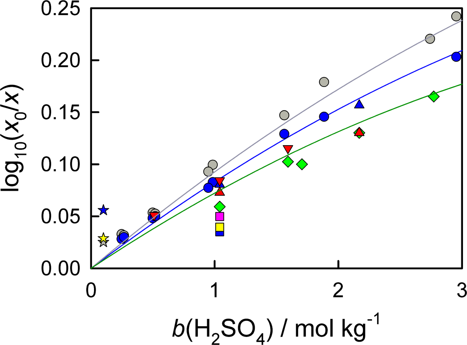
Effect of sulfuric acid on aqueous solubility of oxygen. Experimental data from Geffcken [45] (circles), Narita and Lawson [46] (triangles), Kaskiala [47] (squares), Lang and Zander [48] (diamonds), Kolny and Zembura [49] (stars), and Bruhn et al. [50] (triangles down): gray, 288 K; blue, 298 K; green, 310 K; yellow, 313 K; red, 323 K; purple, 328 K. Lines are calculated using eq. 20 at corresponding temperatures.

HNO₃ + CO₂.

The results by Geffcken [45] in the molality range (0 to 2.54) mol⋅kg⁻¹ and temperatures (288.15 and 298.15) K (Figure 4) were used to derive the equation:

$$k\left({\text{HNO}}_3\right)=-9.332\times {10}^{-3}+52.46\left(\frac{1}{T/\text{K}}-\frac{1}{298.15}\right)$$ (21)

The value by Onda et al. [51] at $T_{\text{h}}$ is consistent with Eq. 21.

Figure 4:

Effect of nitric acid on aqueous solubility of carbon dioxide. Experimental data from Geffcken [45] (circles) and Onda et al. [51] (triangles): blue, 288 K; yellow, 298 K. Lines are calculated with Eq. 21 at corresponding temperatures.

H₂SO₄ + CO₂.

The experimental data [45, 52, 53] are available in the temperature range of (288 to 350) K and at any acid content. Out of these results, the values in the temperature range (288 to 311) K and the molality range (0 to 3) mol. Kg⁻¹ are of interest for this work (Figure 5). Both Geffcken [45] and Shchennikova et al. [53] report that the Sechenov salt effect parameter decreases when the temperature increases. The results by Shchennikova et al. [53] have a relatively large scatter, sometimes have the same magnitude as the salting-out effect itself. Therefore, the resulting equation

$$k\left({\text{H}}_2{\text{SO}}_4\right)=0.06357-9.606\times {10}^{-3}\cdot b_{{\text{H}}_2{\text{SO}}_4}+77.71\left(\frac{1}{T/\text{K}}-\frac{1}{298.15}\right)$$ (22)

was obtained using the data of Geffcken [45] and Markham and Kobe [52].

Figure 5:

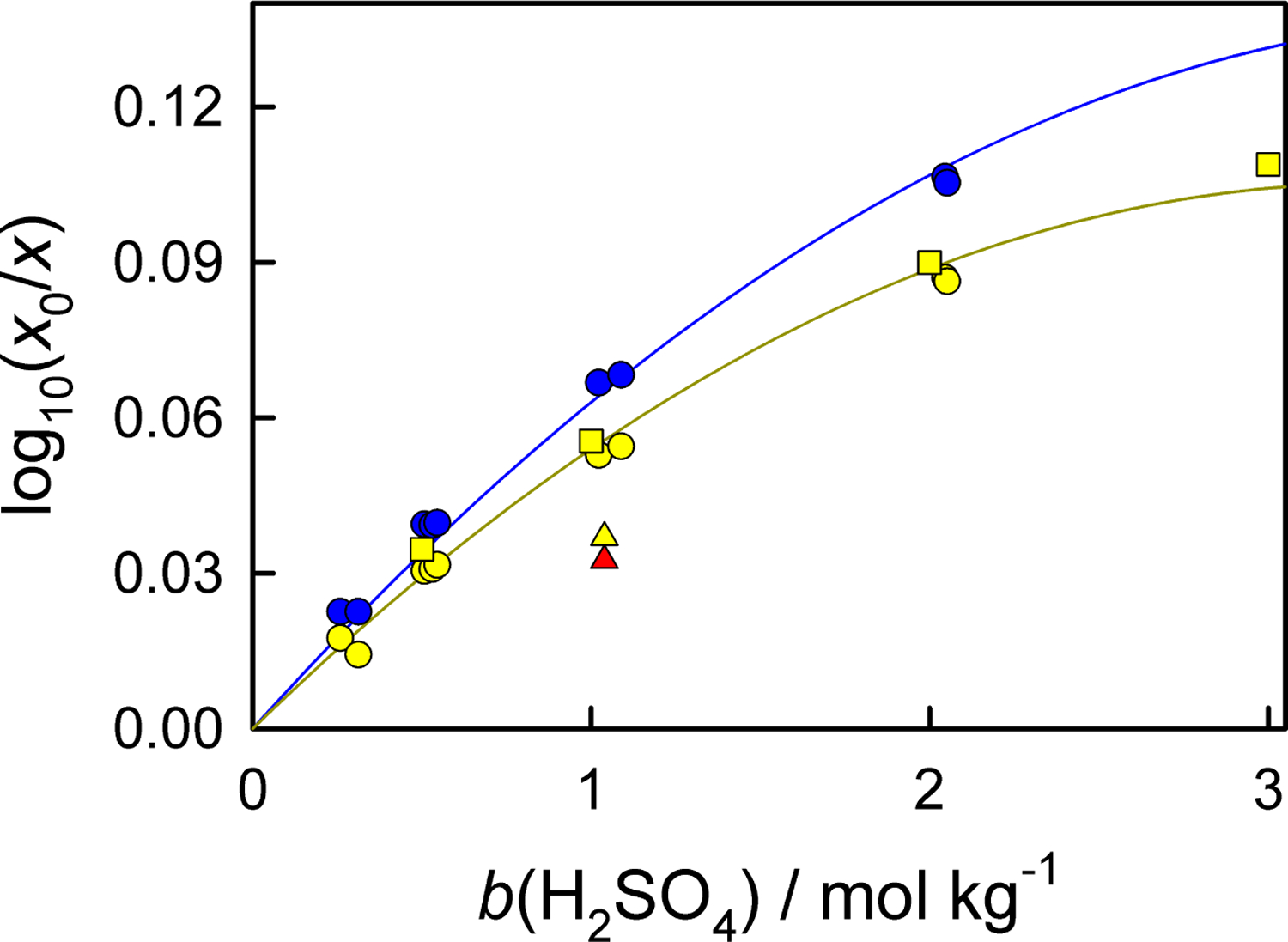
Effect of sulfuric acid on aqueous solubility of carbon dioxide. Experimental data from Geffcken [45] (circles), Markham and Kobe [52] (squares), and Shchennikova et al. [53] (triangles): blue, 288 K; yellow, 298 K; red, 313 K. For Ref. [53], the data are interpolated from the experimental results at different temperatures. Lines are calculated with Eq. 22 at corresponding temperatures

When composition of the liquid phase is available, the gas-phase composition and pressure are refined using Eqs. 7–11 and the virial equation. The activity of water $g$ is found using the model of Carslaw et al. [54], which is adequate for computation of component activities for the HNO₃ + H₂SO₄ + H₂O mixture and its binary endpoints at T = 298.15 K.

2.4. Evaluation of thermal properties (steps 68 to 100)

To find the standard specific energy of combustion, the energy of an isothermal bomb process is first calculated:

$${\Delta }_{\text{IBP}}u=\epsilon \left(t_{\text{i}}-t_{\text{f}}+\Delta t_{\text{corr}}\right)+{\epsilon }_{\text{cont}}^{\text{i}}\left(t_{\text{i}}-t_{\text{h}}\right)+{\epsilon }_{\text{cont}}^{\text{f}}\left(t_{\text{h}}-t_{\text{f}}+\Delta t_{\text{corr}}\right)+{\Delta }_{\text{ign}}u$$ (23)

Here, $\epsilon$ is the energy equivalent of the calorimeter; $t_{\text{i}}$ and $t_{\text{f}}$ are the temperatures in the middle of the initial and final periods; $\Delta t_{\text{corr }}$ is the temperature correction; and ${\Delta }_{\text{ign}}u$ is the ignition energy. All these quantities are determined experimentally and not discussed in this work. It is important to define the sign of $\Delta t_{\text{corr }}$ exactly as proposed in Ref. [5].

Heat capacities of the calorimeter contents, ${\epsilon }_{\text{cont}}$, at $T_{\text{h}}$ in the initial (superscript i) and final (superscript f) periods are estimated with the following equations:

$${\epsilon }_{\text{cont }}^{\text{i}}=C_V\left({\text{O}}_2\right)n^{\text{i}}\left({\text{O}}_2,\text{ tot }\right)+c_P\left({\text{H}}_2\text{O}\right)m^{\text{i}}\left({\text{H}}_2\text{O},\text{ tot }\right)+B{n}^{\text{i}}\left({\text{H}}_2\text{O},\text{ vap }\right)+c_P\left(\text{Pt}\right)m\left(\text{Pt}\right)+c_P\left(\text{ glass }\right)m\left(\text{ glass }\right)+\sum _{\text{compounds }}{c}_{P,i}{m}_i$$ (24)

$${\epsilon }_{\text{cont }}^{\text{f}}=C_V\left({\text{O}}_2+{\text{CO}}_2\right)\left(n^{\text{f}}\left({\text{O}}_2,\text{ tot }\right)+n^{\text{f}}\left({\text{N}}_2,\text{ tot }\right)+n^{\text{f}}\left({\text{CO}}_2,\text{ tot }\right)\right)+\Delta C_V{n}^{\text{f}}\left({\text{N}}_2,\text{ tot }\right)+c_P\left(\text{ soln }\right)+\left(\frac{M\left({\text{H}}_2\text{O}\right)c_P\left(\text{ soln }\right)}{m^{\text{f}}\left(\text{soln}\right)}+B\right)n^{\text{f}}\left({\text{H}}_2\text{O},\text{ vap }\right)+c_P\left(\text{Pt}\right)m\left(\text{Pt}\right)+c_P\left(\text{ glass }\right)m\left(\text{ glass }\right)$$ (25)

Here, the partial heat capacities of dissolved gases are assumed to be equal to those in the gas phase; the contributions due to the temperature dependence of gas solubilities are neglected. The heat capacities for the initial and final states refer to the initial and final pressures, respectively. The temperature dependence can also be considered. Typically, the information required to do these calculations is only partially available and reasonable approximations are introduced.

To obtain equations for the gas-phase heat capacity, the equation of state for (O₂ + CO₂) [55] and the pure-compound equations of state as implemented in REFPROP were used. In the temperature and pressure ranges of (288 to 308) K and (2 to 4) MPa, respectively, the isochoric heat capacity of O₂ is described by the equation

$$C_V\left({\text{O}}_2\right)/\left(\text{J}\cdot {\text{K}}^{-1}\cdot {\text{mol}}^{-1}\right)=21.30+0.077\left(\left(P/\text{MPa}\right)-3\right)+2.8\cdot {10}^{-3}\left(T-298.15\right)$$ (26)

The following equation describes the heat capacity of (O₂ + CO₂) in the same temperature and pressure ranges with the deviations from the values derived with the equation of state below ± 0.08 J⋅K^–1 mol⁻¹:

$$C_V\left({\text{O}}_2+{\text{CO}}_2\right)=C_V\left({\text{O}}_2\right)(1+a_{1}x\left(1+a_2\left(\left(T/K\right)-298.15\right)\right)+a_3{x}^2\left(1+a_4{(\left(\text{P}/\text{MPa}\right)-3)}^2\right))$$ (27)

where $a_1=0.382,a_2=2.54\cdot {10}^{-3},a_3=0.0982,a_4=0.462$, and $x$ is the mole fraction of CO₂. $\Delta C_V=-0.28\text{ J}\cdot {\text{K}}^{-1}\cdot {\text{mol}}^{-1}$ is the average difference between the isochoric heat capacities of N₂ and O₂ in the considered temperature and pressure ranges. Deviation from the average value do not exceed ±0.05 J·K⁻¹·mol⁻¹

The specific isobaric heat capacity of water at $P=3.0\text{ MPa}$ and $T=298.15$ K is $c_P\left({\text{H}}_2\text{O}\right)=4.1731\text{ J}\cdot {\text{K}}^{-1}\cdot {\text{g}}^{-1}$ [14]. In the temperature and pressure ranges of interest, the $c_P$ values deviate from this value by < ±0.17%. This deviation can be ignored because, for other condensed-phase compounds present in the bomb, the values of the isobaric heat capacity are generally available only at $P=0.1\text{MPa}$ and T = 298.15 K. The heat capacities of platinum $c_P\left(\text{Pt}\right)=0.1325\text{ J}\cdot {\text{K}}^{-1}\cdot {\text{g}}^{-1}$ and glass $c_P$ (glass) = 0.71 J⋅K⁻¹⋅g⁻¹ were taken from Refs. [56] and [5], respectively. Summation over compounds includes the main and auxiliary compounds used in an experiment.

The $B$ coefficient in Eqs. 24 and 25 describes the heat capacity contribution due to vaporization of water. Using Hoge’s approach [57], the vaporization correction can be found with the equation:

$${\Delta }_{\text{vap}}c=T\left(\frac{d\left(V_{\text{g}}d{P}_{\text{s}}/dT\right)}{dT}\right)$$ (28)

Assuming the gas volume $V_{\text{g}}$ weakly depends on temperature, the vapor behaves as an ideal gas, and eq. (8) holds, the following transformations are conducted:

$$\begin{gathered} {\Delta }_{\text{vap}}c\approx T{V}_{\text{g}}\left[\frac{d{P}_{\text{s}}}{dT}\left(-\frac{A_1}{T^2}+\frac{A_2}{T}\right)+P_{\text{s}}\left(\frac{2A_1}{T^3}-\frac{A_2}{T^2}\right)\right] \\ =T{V}_{\text{g}}{P}_{\text{s}}\left[{\left(-\frac{A_1}{T^2}+\frac{A_2}{T}\right)}^2+\left(\frac{2A_1}{T^3}-\frac{A_2}{T^2}\right)\right] \\ \approx n^{\text{f}}\left({\text{H}}_2\text{O},\text{vap}\right)R\left[{\left(-\frac{A_1}{T}+A_2\right)}^2+\left(\frac{2A_1}{T}-A_2\right)\right] \\ =n^{\text{f}}\left({\text{H}}_2\text{O},\text{vap}\right)B \end{gathered}$$ (29)

Here, $A_i$ are the coefficients of eq. 8.

The heat capacity of the final solution $c_P$ (soln) is found as

$$c_P\left(\text{ soln }\right)=c_P\left({\text{H}}_2\text{O}\right)m^{\text{f}}\left({\text{H}}_2\text{O}\right)+C_P\left({\text{H}}_2{\text{SO}}_4\right)n^{\text{f}}\left({\text{H}}_2{\text{SO}}_4\right)+C_P\left({\text{HNO}}_3\right)n^{\text{f}}\left({\text{HNO}}_3\right)$$ (30)

where $m^{\text{f}}\left({\text{H}}_2\text{O}\right),n^{\text{f}}\left({\text{H}}_2{\text{SO}}_4\right)$, and $n^{\text{f}}\left({\text{HNO}}_3\right)$ are the mass of water and amounts of acids in the liquid phase, respectively. The apparent heat capacity $C_P\left({\text{H}}_2{\text{SO}}_4\right)$ is calculated using interpolating equations for the molality ranges 0 to 0.02 mol⋅kg⁻¹,

$$C_P\left({\text{H}}_2{\text{SO}}_4\right)/\left(\text{J}\cdot {\text{K}}^{-1}\cdot {\text{mol}}^{-1}\right)=\frac{-286.2-658.57x+33642x^2}{1+3.7413x+444.18x^2},$$ (31)

0.02 to 1.8 mol⋅kg⁻¹,

$$C_P\left({\text{H}}_2{\text{SO}}_4\right)/\left(\text{J}\cdot {\text{K}}^{-1}\cdot {\text{mol}}^{-1}\right)=27.85+20.570x+10.268x^2+\frac{8.9759}{x}-\frac{1.3310}{x^2},$$ (32)

and 1.8 to 6.0 mol⋅kg⁻¹,

$$C_P\left({\text{H}}_2{\text{SO}}_4\right)/\left(\text{J}\cdot {\text{K}}^{-1}\cdot {\text{mol}}^{-1}\right)=\frac{-71.76-87.255x+31.085x^2}{1-1.1815x+0.39918x^2},$$ (33)

where $x=\sqrt{b_{{\text{H}}_2{\text{SO}}_4}}$. These equations interpolate values given in Table 8 of Ref. [58] within ±0.6 J⋅K⁻¹⋅mol⁻¹.

The apparent heat capacity $C_P\left({\text{HNO}}_3\right)$ is found with interpolating equations for the molality ranges 0 to 0.45 mol⋅kg⁻¹,

$$C_P\left({\text{HNO}}_3\right)/\left(\text{J}\cdot {\text{K}}^{-1}\cdot {\text{mol}}^{-1}\right)=-72.0+28.8705x+5.50256x^2,$$ (34)

and 0.45 to 6.9 mol⋅kg⁻¹,

$$C_P\left({\text{HNO}}_3\right)/\left(\text{J}\cdot {\text{K}}^{-1}\cdot {\text{mol}}^{-1}\right)=-61.81+27.9759x^2-2.48030x^4+0.112509x^6.$$ (35)

where $x=\sqrt{b_{{\text{HNO}}_3}}$. Using Eqs. 34 and 35 to interpolate values reported in Table V of Ref. [59] provides fitted values within ±0.4 J⋅K⁻¹⋅mol⁻¹.

The energy of combustion of a compound under bomb conditions is defined as follows:

$${\Delta }_{\text{B}}u={\Delta }_{\text{IBP}}u+{\Delta }_{\text{decomp }}{U}_{\text{m}}\left({\text{HNO}}_3\right)n_{\text{f}}\left({\text{HNO}}_3\right)+{\Delta }_{\text{c}}u\left(\text{ soot }\right)m\left(\text{ soot }\right)-\sum _{i>1}{\Delta }_{\text{c}}{u}_i^{\circ }{m}_i$$ (36)

where ${\Delta }_{\text{c}}{u}_i^{\circ }$ and $m_i$ are the standard specific energies of combustion and masses of the auxiliary compounds.

As presented in the NBS Tables [60], decomposition of 0.1 mol⋅kg⁻¹ aqueous nitric acid into water and gaseous elements is accompanied by a thermal effect of ${\Delta }_{\text{decomp }}{U}_{\text{m}}^{\circ }=59.7\text{ kJ}\cdot {\text{mol}}^{-1}$. This quantity is adjusted to the real molality of the final solution using the dilution enthalpies described below and used in eq. 36.

Sometimes, a small amount of soot is found in the products. The energy of combustion for soot is calculated as that for pure graphite (${\Delta }_{\text{c}}{u}^{\circ }=-32.76\text{ J}\cdot {\text{g}}^{-1}$ [61]). This may introduce an error of as large as 5% to this contribution. However, since the mass of soot is normally well below 1 mg, this assumption is acceptable. The term associated with soot was absent in the original description of the procedures. [5]

The standard specific energy of combustion of the main compound is a sum of two terms divided by the mass of the main compound, $m_1$ :

$${\Delta }_{\text{c}}{u}^{\circ }=\left({\Delta }_{\text{B}}u+\Delta u_{\text{corr }}\right)/m_1$$ (37)

The second term in Eq. 37 describes the corrections to the standard state. It is a combination of the following contributions:

$$\text{Δ}{u}_{\text{corr }}={\text{Δ}}_{\text{vap }}U\left({\text{H}}_2\text{O}\right)n^{\text{i}}\left({\text{H}}_2\text{O gas }\right) +\left[P^{\text{i}}\left(\text{gas }\right)-P^{\circ }\right]{\left(\frac{\partial U\left({\text{H}}_2\text{O liq }\right)}{\partial P}\right)}_T{n}^{\text{i}}\left({\text{H}}_2\text{O liq }\right)+\left[P^{\text{i}}\left(\text{ gas }\right)-P^{\circ }\right]\sum _i{m}_i{\left(\frac{\partial u_i}{\partial P}\right)}_T+P^{\text{i}}\left(\text{ gas }\right){\left(\frac{\partial U\left({\text{O}}_2\text{ gas }\right)}{\partial P}\right)}_T{n}^{\text{i}}\left({\text{O}}_2\text{ gas }\right)+{\text{Δ}}_{\text{sol }}U\left({\text{O}}_2\right)n^{\text{i}}\left({\text{O}}_2\text{ diss. }\right)-{\text{Δ}}_{\text{sol }}U\left({\text{CO}}_2\right)n^{\text{f}}\left({\text{CO}}_2\text{ diss. }\right)-{\text{Δ}}_{\text{sol }}U\left({\text{O}}_2\right)n^{\text{f}}\left({\text{O}}_2\text{ diss. }\right)-{\text{Δ}}_{\text{sol }}U\left({\text{ N}}_2\right)n^{\text{f}}\left({\text{N}}_2\text{ diss. }\right)+\left[P^{\circ }-P^{\text{f}}\left(\text{gas }\right)\right]{\left(\frac{\partial U\left(\text{ soln }\right)}{\partial P}\right)}_T{m}^{\text{f}}\left(\text{ soln }\right)+{\text{Δ}}_{\text{diln }}U\left({\text{HNO}}_3\right)n^{\text{f}}\left({\text{HNO}}_3\right)+{\text{Δ}}_{\text{diln }}U\left({\text{H}}_2{\text{SO}}_4\right)n^{\text{f}}\left({\text{H}}_2{\text{SO}}_4\right)-P^{\text{f}}\left(\text{ gas }\right){\left(\frac{\partial U\left(\text{ gas }\right)}{\partial P}\right)}_T^{\text{f}}\left(\text{ gas }\right)-{\text{Δ}}_{\text{vap }}U\left({\text{H}}_2\text{O}\right)n^{\text{f}}\left({\text{H}}_2{\text{O}}_{\text{gas }}\right)$$ (38)

Numerical values of all terms in eq. 38 for the benzoic acid and 3-methylthiophene examples can be found in Supplementary Material. For all instances, partial derivatives of internal energy with respect to pressure are estimated as

$${\left(\frac{\partial U}{\partial P}\right)}_T=-T{\left(\frac{\partial V}{\partial T}\right)}_P$$ (39)

where the derivative is assumed to be pressure-independent. For gases, Eqn. 39 transforms into

$${\left(\frac{\partial U}{\partial P}\right)}_T=-T{\left(\frac{\partial B_{\text{mix}}}{\partial T}\right)}_P.$$ (40)

The use of Eq. 40 introduces an error of < 1% relative to the rigorous calculations. For the condensed phases, the error of Eq. 39 is difficult to evaluate since the input quantity ${\left(\frac{\partial V}{\partial T}\right)}_P$ is often an estimate itself. However, this is typically not a problem since the contributions associated with compressibility of gases are two orders of magnitude larger than those of condensed phases.

Preliminary tests for the calculation of enthalpies of dilution for

$${\text{HNO}}_3\left(\text{aq},b_{{\text{HNO}}_3}\right)\to {\text{HNO}}_3\left(\text{aq},0.1\text{mol}\cdot {\text{kg}}^{-1}\right)$$ (41)

$${\text{H}}_2{\text{SO}}_4\left(\text{aq},b_{{\text{H}}_2{\text{SO}}_4}\right)\to {\text{H}}_2{\text{SO}}_4\left(\cdot 115{\text{H}}_2\text{O}\right)$$ (42)

demonstrated that the model by Carslaw et al. [54] for the (HNO₃ + H₂ SO₄ + H₂O) mixture has unacceptable deviation from the experimental dilution enthalpies for both acids. Thus, the enthalpies of processes described by Eqs. 41 and 42 have to be found independently.

The most precise experimental data for H₂SO₄ have been reported by Wu and Young [62]. They recommended apparent enthalpies, $L\left({\text{H}}_2{\text{SO}}_4\right)$, based on their experimental data as well as the results available in the literature at that time. Below $b_{{\text{H}}_2{\text{SO}}_4}=0.001\text{ mol}\cdot {\text{kg}}^{-1}$, no experimental data was available and a semi-theoretical extrapolation was applied.

The currently accepted enthalpy and equilibrium constant for the HSO4⁻ dissociation [58] at $T=298.15\text{ K}$ are ${\Delta }_{r}H=22.76\text{ kJ}\cdot {\text{mol}}^{-1}$ and $K_{\text{r}}=0.0105$ mol. Kg⁻¹, respectively. For the extrapolation, the activity coefficients of the sulfate ion and apparent enthalpies of the ions are estimated with the Debye-Hückel limiting law. At $b_{{\text{H}}_2{\text{SO}}_4}=0.0016\text{ mol}\cdot {\text{kg}}^{-1}$, the value is 40 J⋅mol⁻¹ higher than the one recommended by Wu and Young. We use this extrapolation below $0.0016\text{ mol}\cdot {\text{kg}}^{-1}$ and the values from Table 5 of Ref. [62] shifted by 40 J⋅mol⁻¹ above it.

The interpolating equations are as follows:

$$L\left({\text{H}}_2{\text{SO}}_4\right)/\left(\text{J}\cdot {\text{mol}}^{-1}\right)=24251.7-\frac{2041.761}{x}+\frac{88.77421}{x^2}-\frac{2.051916}{x^3}+\frac{0.01959695}{x^4}$$ (43)

$$L\left({\text{H}}_2{\text{SO}}_4\right)/\left(\text{J}\cdot {\text{mol}}^{-1}\right)=15582.5+15565.7x-13918.14x^2+5944.99x^3-778.57x^4;$$ (44)

where $x=\sqrt{b_{{\text{H}}_2{\text{SO}}_4}}$. Eqs. 43 and 44 are valid at the molality ranges of (0.0016 to 0.49) mol⋅kg⁻¹ and (0.49 to 9.0) mol⋅kg⁻¹, respectively. The maximum deviation from the corrected values of Wu and Young is 36 J⋅mol⁻¹ and the standard deviation is 11 J⋅mol⁻¹. The enthalpies of dilution are calculated as a difference of apparent enthalpies at corresponding molalities.

For Eq. 41, the (HNO₃ + H₂O) model by Clegg and Brimblecombe [59] is applied. The apparent enthalpies $L_{{\text{HNO}}_3}$ at $T_{\text{h}}$ tabulated in Table VII of the original paper were approximated within ±0.7 J⋅mol⁻¹ by the equations:

$$L\left({\text{HNO}}_3\right)/\left(\text{J}\cdot {\text{mol}}^{-1}\right)=1939.00x-2824.25x^2+1627.43x^3$$ (45)

$$L\left({\text{HNO}}_3\right)/\left(\text{J}\cdot {\text{mol}}^{-1}\right)=62.05+1484.36x-1628.70x^2+546.541x^3-1.73757x^6$$ (46)

where $x=\sqrt{b_{{\text{HNO}}_3}}$. Eqs. 45 and 46 are valid at the HNO₃ molality ranges of 0 to 0.22 mol⋅kg⁻¹ and 0.22 to 6.9 mol⋅kg⁻¹, respectively.

The molar energies of gas dissolution in water are calculated from the Henry’s law constants:

$$\begin{gathered} {\Delta }_{\text{sol}}{U}^{\circ }=-R{T}^2\frac{d\text{\hspace{0.17em}ln\hspace{0.17em}}{k}_{\text{H}}}{dT}+RT \\ =R\left(b+\frac{2c}{T}+T\right) \end{gathered}$$ (47)

The $b$ and $c$ coefficients are listed in Table 2. Eq. 47 is extended for gas dissolution in acidic solutions,

$${\Delta }_{\text{sol}}{U}^{\circ }=R(b+\frac{2c}{T}+T-T^2\text{\hspace{0.17em}ln\hspace{0.17em}}10(b\left({\text{H}}_2{\text{SO}}_4\right)\frac{dk\left({\text{H}}_2{\text{SO}}_4\right)}{dT}+b\left({\text{HNO}}_3\right)\frac{dk\left({\text{HNO}}_3\right)}{dT}))$$ (48)

where $k$ is provided by Eqs. 19–22. The change of internal energy for vaporization of water is ${\Delta }_{\text{vap }}{U}^{\circ }\left({\text{H}}_2\text{O}\right)=41.53\text{ J}\cdot {\text{mol}}^{-1}$ at $T_{\text{h}}$. [61]

The largest differences with the 1956 formulation include gas compression/decompression (steps 85 and 93), oxygen solution/dissolution (steps 84 and 88), and carbon dioxide dissolution (step 87). The changes are about −3 %, −40 %, and +10 %, respectively. Steps 85 and 93 are by far the largest contributions. The second pair of contributions is lower by more than an order of magnitude than the first one. However, a large decrease of the enthalpies of dissolution makes the change also significant. Within these pairs, the contributions are partially cancelled. The difference with the 1956 results will increase with the increasing pressure difference between the initial and final states. The changes for step 87 are also comparable with those for the pairs. Typically, the standard energies of combustion change by several J.g⁻¹ relative to the 1956 formulation.

While the described procedures are mathematically not very complicated, their implementation is time-consuming and prone to failure. A rigorously tested standard web-based tool that implements these procedures for convenient application is described next.

3. Web-based tool

A single-page web application that implements the procedures described above is freely available at https://trc.nist.gov/cctool/. [2] All that is required to use the web-based tool is a JavaScript enabled web browser and an internet connection. Once served, all calculations run on the client using JavaScript. The Vue web framework [63] is used to provide user interface reactivity that enables continuous validation of parameters and seamless switching between different modes (calibration and experiment) and options (e.g., using buoyancy corrected masses or balance readings) for calculations. Continuous validations are used to constrain entered values to reasonable ranges. For example, the pressure of O₂ must be (2 to 4) MPa. The tool has three tabs: the Calorimeter tab, the Compounds tab, and the Help tab.

The Calorimeter tab (Figure 6) provides a form with 15 or 16 parameters (depending on the buoyancy correction switch) associated with the experimental setup and conditions. It also provides a selection menu for the calorimeter mode (Experiment or Calibration) and buttons to save/load the state of the tool, display the report (described below), and reset the tool. The Save button will package the state of the tool and download a JSON file to the user file system. The JSON file can then be used to reload the calorimeter state by dragging and dropping the file on to the load button. The load button also supports file system navigation.

Figure 6:

Calorimeter tab of the Combustion Calorimetry Tool

The Compounds tab (Figure 7) has 24 parameters for three auxiliary compounds and 9 (experiment mode) or 10 parameters (calibration mode) for the main compound. Auxiliary compounds may contain only C, H, and O atoms while the main compound may contain those along with N and S. The molar mass and molecular formula are read-only values that continuously update with changes to the number of entered atoms.

Figure 7:

Compounds tab of the Combustion Calorimetry Tool

The Help tab contains brief description of the working procedures, downloadable examples of experiments and calibrations that can be used to get oriented with the tool. The examples are JSON files that can be used as described above.

The report (Figure 8), accessed from the Calorimeter tab, contains the information necessary to make the experiment and calculations traceable and verifiable. The report may be downloaded to the user’s computer in a csv format that can be loaded in an Excel spreadsheet. Well-executed studies contain similar tables for at least one experiment of a series. However, there are a considerable number of papers where this information is lost. Without intermediate results, possible errors and inconsistencies become hidden and the results become essentially useless. The NIST combustion calorimetry tool provides a convenient way to generate and save the expanded tables that include all essential information. Furthermore, these files (reports and the loadable state) could be easily submitted as supporting information for publications. The use of this tool will reduce a number of arithmetic errors in the computations and the final result and facilitate interlaboratory communication.

Figure 8:

Report of the Combustion Calorimetry Tool - Experiment Mode

4. Conclusions

Standard enthalpies of formation for organic compounds are generally determined from combustion calorimetry experiments conducted at a pressure close to 3 MPa. Correcting the results to the standard state is critical to the determination of useful enthalpies of formation. The original procedure was proposed in 1956 and is improved in this work.

The current work provides a correction procedure that avoids unnecessary simplifications and is more suitable for computer implementation. The pressure-based virial equation is explicitly used in all calculations for gas mixtures. Multiple tables are replaced with thermodynamic models and accurate interpolating functions. The reference values are updated using primary sources published by 2020. Compared to the original correction procedure, some contributions, such as gas compression/decompression, gas solubilities, and energies of solution of gases in pure water), are changed by several joules per 1 g of the burnt material (main and auxiliary compounds). Updated values of the standard energy of combustion are typically within 1 kJ⋅mol⁻¹ of those determined with the previous procedure.

Uncertainty of the correction term is hard to estimate. We believe the relative expanded uncertainty (0.95 level of confidence) to be a few per cent. State-of-the-art values used in the current work include: the virial coefficients of gases and their mixtures; gas solubilities and energies of solution of gases in pure water; reference values for water and platinum. Further improvement of these reference values is not required. The uncertainty for N- and S-containing compounds can be decreased if new experimental data on O₂, CO₂, and N₂ solubilities in aqueous HNO₃ and H₂SO₄ are available. An accurate thermodynamic model for (HNO₃ + H₂SO₄ + H₂O) will benefit measurements of SN-containing compounds.

The updated algorithm is presented in the form of a Web-based tool available through the NIST TRC Web site. This tool can be used to check consistency of the in-house software created in different laboratories. The files saved with this tool can be used for data exchange between laboratories and submitted as supporting information for publications. The generated report has essential information that is recommended for inclusion in the data tables of combustion calorimetry papers.

References

- [1].Sabbah R, Xu-wu A, Chickos JS, Planas Leitão ML, Roux MV, Torres LA, Reference Materials for Calorimetry and Differential Thermal Analysis, Thermochim. Acta 331 (1999) 93–204. doi: 10.1016/S0040-6031(99)00009-X. [DOI] [Google Scholar]
- [2].Paulechka E, Riccardi D, NIST Standard Reference Database 206: Combustion Calorimetry Tool, National Institute of Standards and Technology (2020). doi: 10.18434/M32043. URL https://trc.nist.gov/cctool [DOI] [Google Scholar]
- [3].Diky V, Bazyleva A, Paulechka E, Magee JW, Martinez V, Riccardi D, Kroenlein K, Validation of thermophysical data for scientific and engineering applications, J. Chem. Thermodyn 133 (2019) 208–222. doi: 10.1016/jjct.2019.01.029. [DOI] [PMC free article] [PubMed] [Google Scholar]
- [4].Paulechka E, Kazakov A, Critical Evaluation of the Enthalpies of Formation for Fluorinated Compounds Using Experimental Data and High-Level Ab Initio Calculations, J. Chem. Eng. Data 64 (2019) 4863–4875. doi: 10.1021/acs.jced.9b00386. [DOI] [PMC free article] [PubMed] [Google Scholar]
- [5].Hubbard WN, Scott DW, Waddington G, Experimental Thermochemistry, Vol. 1, Interscience Publishers, New York, 1956, Ch. 5. Standard States and Corrections for Combustions in a Bomb at Constant Volume. [Google Scholar]
- [6].Good WD, Scott DW, Experimental Thermochemistry, Vol. 2, Interscience Publishers, New York, 1962, Ch. 2. Combustion in a Bomb of Organic Fluorine Compounds. [Google Scholar]
- [7].Hajiev SN, Agarunov MJ, Nurullaev HG, p-chlorobenzoic Acid. Determination of Enthalpy of Combustion in the Presence of Hydrazine Di-hydrochloride, J. Chem. Thermodyn 6 (1974) 713–725. doi: 10.1016/0021-9614(74)90135-9. [DOI] [Google Scholar]
- [8].Bjellerup L, Experimental Thermochemistry, Vol. 2, Interscience Publishers, New York, 1962, Ch. 3. Combustion in a Bomb of Organic Bromine Compounds. [Google Scholar]
- [9].Hajiev SN, Bomb Calorimetry, Khimiya, Moscow, 1988. [Google Scholar]
- [10].Månsson M, Hubbard WN, Combustion Calorimetry, Vol. 1 of Expeirmental Chemical Thermodynamics, Pergamon Press, New York, 1979, Ch. 5. Strategies in the Calculation of Standard-State Energies of Combustion from the Experimentally Determined Quantitites. [Google Scholar]
- [11].Weighing the Right Way, Mettler Toledo, 2015. [Google Scholar]
- [12].Picard A, Davis RS, Glser M, Fujii K, Revised formula for the density of moist air (CIPM-2007), Metrologia 45 (2008) 149–155. doi: 10.1088/0026-1394/45/2/004. [DOI] [Google Scholar]
- [13].Meija J, Coplen TB, Berglund M, Brand WA, De Bièvre P, Gröning M, Holden NE, Atomic weights of the elements 2013 (IUPAC Technical Report), Pure Appl. Chem 88 (2016) 265–291. doi: 10.1515/pac-2015-0305. [DOI] [Google Scholar]
- [14].International Association for the Properties of Water and Steam, Revised Release on the IAPWS Formulation 1995 for the Thermodynamic Properties of Ordinary Water Substance for General and Scientific Use (2018). URL http://www.iapws.org/relguide/IAPWS95-2018.pdf
- [15].Wagner W, Pruß A, The IAPWS Formulation 1995 for the Thermodynamic Properties of Ordinary Water Substance for General and Scientific Use, J. Phys. Chem. Ref. Data 31 (2002) 387–535. doi: 10.1063/1.1461829. [DOI] [Google Scholar]
- [16].Lemmon EW, Bell IH, Huber ML, McLinden MO, NIST Standard Reference Database 23: Reference Fluid Thermodynamic and Transport Properties-REFPROP, Version 10.0, National Institute of Standards and Technology; (2018). doi: 10.18434/T4/1502528. URL https://www.nist.gov/srd/refprop [DOI] [Google Scholar]
- [17].Schmidt R, Wagner W, A new form of the equation of state for pure substances and its application to oxygen, Fluid Phase Equilib. 19 (1984) 175–200. doi: 10.1016/0378-3812(85)87016-3. [DOI] [Google Scholar]
- [18].Martin ML, Trengove RD, Harris KR, Dunlop PJ, Excess second virial coefficients for some dilute binary gas mixtures, Aust. J. Chem 35 (1982) 1525–1529. doi: 10.1071/CH9821525. [DOI] [Google Scholar]
- [19].Cottrell TL, Hamilton RA, Taubinger RP, The second virial coefficients of gases and mixtures. part 2. – Mixtures of carbon dioxide with nitrogen, oxygen, carbon monoxide, argon and hydrogen, Trans. Faraday Soc 52 (1956) 1310–1312. [Google Scholar]
- [20].Hellmann R, Reference Values for the Cross Second Virial Coefficients and Dilute Gas Binary Diffusion Coefficients of the Systems (H2O + O2) and (H2O + Air) from First Principles, J. Chem. Eng. Data 65 (2020) (in press). [DOI] [PMC free article] [PubMed] [Google Scholar]
- [21].Span R, Wagner W, A New Equation of State for Carbon Dioxide Covering the Fluid Region from the Triple-Point Temperature to 1100 K at Pressures up to 800 MPa, J. Phys. Chem. Ref. Data 25 (1996) 1509–1596. doi: 10.1063/1.555991. [DOI] [Google Scholar]
- [22].Crusius J-P, Castro-Palacio RHJC, Vesovic V, Ab initio inter-molecular potential energy surface for the CO2-N2 system and related thermophysical properties, J. Chem. Phys 148 (2018) 214306. doi: 10.1063/1.5034347. [DOI] [PubMed] [Google Scholar]
- [23].Meyer CW, Harvey AH, Dewpoint measurements for water in compressed carbon dioxide, AIChE J. 61 (2015) 2913–2925. doi: 10.1002/aic.14818. [DOI] [Google Scholar]
- [24].Span R, Lemmon EW, Jacobsen RT, Wagner W, Yokozeki A, A Reference Equation of State for the Thermodynamic Properties of Nitrogen for Temperatures from 63.151 to 1000 K and Pressures to 2200 MPa, J. Phys. Chem. Ref. Data 29 (2000) 1361–1433. doi: 10.1063/1.1349047. [DOI] [Google Scholar]
- [25].Hellmann R, First-Principles Calculation of the Cross Second Virial Co-efficient and the Dilute Gas Shear Viscosity, Thermal Conductivity, and Binary Diffusion Coefficient of the (H2O + N2) System, J. Chem. Eng. Data 64 (2019) 5959–5973. doi: 10.1021/acs.jced.9b00822. [DOI] [Google Scholar]
- [26].Hellmann R, Correction to first-Principles Calculation of the Cross Second Virial Coefficient and the Dilute Gas Shear Viscosity, Thermal Conductivity, and Binary Diffusion Coefficient of the (H2O + N2) System, J. Chem. Eng. Data 65 (2020) 2251–2252. doi: 10.1021/acs.jced.0c00248. [DOI] [Google Scholar]
- [27].Harvey AH, Lemmon EW, Correlation for the Second Virial Coefficient of Water, J. Phys. Chem. Ref. Data 33 (2004) 369–376. doi: 10.1063/1.1587731. [DOI] [Google Scholar]
- [28].Rettich TR, Battino R, Wilhelm E, Solubility of Gases in liquids. xvi. Henry’s Law Coefficients for Nitrogen in Water at 5 to 50° C, J. Solut. Chem 13 (1984) 335–348. doi: 10.1007/BF00645706. [DOI] [Google Scholar]
- [29].Rettich TR, Battino R, Wilhelm E, Solubility of gases in liquids. 22. High-precision determination of Henrys law constants of oxygen in liquid water from T = 274 K to T = 328 K, J. Chem. Thermodyn 32 (2000) 1145–1156. doi: 10.1006/jcht.1999.0581. [DOI] [Google Scholar]
- [30].Crovetto R, Evaluation of Solubility Data of the System CO2 –H2O from 273 K to the Critical Point of Water, J. Phys. Chem. Ref. Data 20 (1991) 575–589. doi: 10.1063/1.555905. [DOI] [Google Scholar]
- [31].Kell GS, Effects of isotopic composition, temperature, pressure, and dissolved gases on the density of liquid water, J. Phys. Chem. Ref. Data 6 (1977) 1109–1131. doi: 10.1063/1.555561. [DOI] [Google Scholar]
- [32].Zhou T, Battino R, Partial Molar Volumes of 13 Gases in Water at 298.15 K and 303.15 K, J. Chem. Eng. Data 46 (2001) 331–332. doi: 10.1021/je000215o. [DOI] [Google Scholar]
- [33].Enns T, Scholander PF, Bradstreet ED, Effect of Hydrostatic Pressure on Cases Dissolved in Water, J. Phys. Chem 69 (1965) 389–391. doi: 10.1021/j100886a005. [DOI] [PubMed] [Google Scholar]
- [34].Krichevsky IR, Kasarnovsky JS, Thermodynamical Calculations of Solubilities of Nitrogen and Hydrogen in Water at High Pressures, J. Am. Chem. Soc 57 (1935) 2168–2171. doi: 10.1021/ja01314a036. [DOI] [Google Scholar]
- [35].Moore JC, Battino R, Rettlch TR, Handa YP, Wilhelm E, Partial Molar Volumes of Gases at Infinite Dilution in Water at 298.15 K, J. Chem. Eng. Data 27 (1982) 22–24. doi: 10.1021/je00027a005. [DOI] [Google Scholar]
- [36].Bignell N, Partial molar volumes of atmospheric gases in water, J. Phys. Chem 88 (1984) 5409–5412. doi: 10.1021/j150666a060. [DOI] [Google Scholar]
- [37].Kritchevsky I, Iliinskaya A, Partial molar volumes of gases dissolved in liquids. (A contribution to the thermodynamics of dilute solutions of non-electrolytes), Acta Physicochim. U.S.S.R 20 (1945) 327–348. [Google Scholar]
- [38].Tiepel EW, Gubbins KE, Partial molal volumes of gases dissolved in electrolyte solutions, J. Phys. Chem 76 (1972) 3044–3049. doi: 10.1021/j100665a024. [DOI] [Google Scholar]
- [39].Barbero JA, Hepler LG, McCurdy KG, Tremaine PR, Thermodynamics of aqueous carbon dioxide and sulfur dioxide: heat capacities, volumes, and the temperature dependence of ionization, Can. J. Chem 61 (1983) 2509–2519. doi: 10.1139/v83-433. [DOI] [Google Scholar]
- [40].International Critical Tables of Numerical Data, Physics, Chemistry and Technology, Vol. 3, McGraw-Hill Book Company, New York, 1928. [Google Scholar]
- [41].Scharlin P, Cargill RW, Carbon dioxide in water and aqueous electrolyte solutions, Vol. 62 of Solubility Data Series, Oxford University Press, Oxford, UK, 1996. [Google Scholar]
- [42].Battino R, Oxygen and Ozone, Vol. 7 of Solubility Data Series, Pergamon Press, Oxford, UK, 1981. [Google Scholar]
- [43].Clever HL, Battino R, Miyamoto H, Yampolski Y, Young CL, IUPAC-NIST Solubility Data Series. 103. Oxygen and Ozone in Water, Aqueous Solutions, and Organic Liquids (Supplement to Solubility Data Series Volume 7), J. Phys. Chem. Ref. Data 43 (2014) 033102. doi: 10.1063/1.4883876. [DOI] [Google Scholar]
- [44].Pogrebnaya VL, Usov AP, Baranov AV, Machigin AA, Solubility of oxygen in nitric acid, Izv. Vyssh. Uchebn. Zaved. Khim. Khim. Tekhnol 15 (1972) 16–20. [Google Scholar]
- [45].Geffcken G, Beiträge zur Kenntnis der Löslichkeitsbeeinflussung, Z. Phys. Chem 49U (1904) 257–302. doi: 10.1515/zpch-1904-4925. [DOI] [Google Scholar]
- [46].Narita E, Lawson F, Han KN, Solubility of oxygen in aqueous electrolyte solutions, Hydrometallurgy 10 (1983) 21–37. doi: 10.1016/0304-386X(83)90074-9. [DOI] [Google Scholar]
- [47].Kaskiala T, Determination of oxygen solubility in aqueous sulphuric acid media, Miner. Eng 15 (2002) 853–857. doi: 10.1016/S0892-6875(02)00089-4. [DOI] [Google Scholar]
- [48].Lang W, Zander R, Salting-out of oxygen from aqueous electrolyte solutions: prediction and measurement, Ind. Eng. Chem. Fundamen 25 (1986) 775–782. doi: 10.1021/i100024a050. [DOI] [Google Scholar]
- [49].Kolny H, Zembura Z, Solubility and heat of dissolution of oxygen in airsaturated 0.1 M solution of sulfuric acid at 5–75° C, Rochniki Chemii 41 (1967) 639–641. [Google Scholar]
- [50].Bruhn G, Gerlach J, Pawlek F, Untersuchungen über die Löslichkeiten von Salzen und Gasen in Wasser und wäßrigen Lösungen bei Temperaturen oberhalb 100°C, Z. anorg. allgem. Chem 337 (1965) 68–79. doi: 10.1002/zaac.19653370111. [DOI] [Google Scholar]
- [51].Onda K, Sada E, Kobayashi T, Kito S, Ito K, Salting-out parameters of gas solubility in aqueous salt solutions, J. Chem. Eng. Jpn 3 (1970) 18–24. doi: 10.1252/jcej.3.18. [DOI] [Google Scholar]
- [52].Markham AE, Kobe KA, The Solubility of Carbon Dioxide in Aqueous Solutions of Sulfuric and Perchloric Acids at 25°, J. Am. Chem. Soc 63 (1941) 1165–1166. doi: 10.1021/ja01849a507. [DOI] [Google Scholar]
- [53].Shchennikova MK, Devyatykh GG, Korshunov IA, Determination of carbon dioxide solubility in aqueous solutions of sulfuric acid by the method of isotope dilution, Zh. Prikl. Khim 30 (1957) 881–886. [Google Scholar]
- [54].Carslaw KS, Clegg SL, Brimblecombe P, A Thermodynamic Model of the System HCl-HNO3-H2SO4-H2O, Including Solubilities of HBr, from < 200 to 328 K, J. Phys. Chem 99 (1995) 11557–11574. doi: 10.1021/j100029a039. [DOI] [Google Scholar]
- [55].Gernert J, Span R, EOS–CG: A Helmholz energy mixture model for humid gases and CCS mixtures, J. Chem. Thermodyn 93 (2019) 274–293. doi: 10.1016/jjct.2015.05.015. [DOI] [Google Scholar]
- [56].Thermal properties of compounds [cited April 30th, 2020]. URL http://www.chem.msu.ru/cgi-bin/tkv.pl
- [57].Hoge HJ, Heat capacity of a two-phase system, with applications to vapor corrections in calorimetry, J. Res. Nat. Bur. Stand 36 (1946) 111–118. doi: 10.6028/jres.036.003. [DOI] [PubMed] [Google Scholar]
- [58].Clegg SL, Rard JA, Pitzer KS, Thermodynamic Properties of 0–6 mol kg−1 Aqueous Sulfuric Acid from 273.15 to 328.15 K, J. Chem. Soc. Faraday Trans 90 (1994) 1875–1894. doi: 10.1039/FT9949001875. [DOI] [Google Scholar]
- [59].Clegg SL, Brimblecombe P, Equilibrium Partial Pressures and Mean Activity and Osmotic Coefficients of 0–100 % Nitric Acid as a Function of Temperature, J. Phys. Chem 94 (1990) 5369–5380. doi: 10.1021/j100376a038. [DOI] [Google Scholar]
- [60].Wagman DD, Evans WH, Parker VB, Schumm RH, Halow I, Bailey SM, Churney KL, Nuttall RL, The NBS tables of chemical thermodynamic properties. Selected values for inorganic and C1 and C2 organic substances in SI units, J. Phys. Chem. Ref. Data 11, Suppl. 2 (1982) 1–392. [Google Scholar]
- [61].Cox JD, Wagman DD, Medvedev VA, CODATA Key Values for Thermodynamics, Hemisphere Publishing Corp., New York, 1989. [Google Scholar]
- [62].Wu YC, Young TF, Enthalpies of Dilution of Aqueous Electrolytes: Sulfuric Acid, Hydrochloric Acid, and Lithium Chloride, J. Res. Nat. Bur. Stand 85 (1980) 11–17. doi: 10.6028/jres.085.002. [DOI] [PMC free article] [PubMed] [Google Scholar]
- [63].Vue.js, the Progressive JavaScript Framework, https://vuejs.org, accessed: 2020-06-23.
Associated Data
This section collects any data citations, data availability statements, or supplementary materials included in this article.