Behavioral Analytics for Myopic Agents

Abstract

Many multi-agent systems have a single coordinator providing incentives to a large number of agents. Two challenges faced by the coordinator are a finite budget from which to allocate incentives, and an initial lack of knowledge about the utility function of the agents. Here, we present a behavioral analytics approach for solving the coordinator’s problem when the agents make decisions by maximizing utility functions that depend on prior system states, inputs, and other parameters that are initially unknown. Our behavioral analytics framework involves three steps: first, we develop a model that describes the decision-making process of an agent; second, we use data to estimate the model parameters for each agent and predict their future decisions; and third, we use these predictions to optimize a set of incentives that will be provided to each agent. The framework and approaches we propose in this paper can then adapt incentives as new information is collected. Furthermore, we prove that the incentives computed by this approach are asymptotically optimal with respect to a loss function that describes the coordinator’s objective. We optimize incentives with a decomposition scheme, where each sub-problem solves the coordinator’s problem for a single agent, and the master problem is a pure integer program. We conclude with a simulation study to evaluate the effectiveness of our approach for designing a personalized weight loss program. The results show that our approach maintains efficacy of the program while reducing its costs by up to 60%, while adaptive heuristics provide substantially less savings.

1. Introduction

The increasing availability of data presents an opportunity to transform incentive design (i.e., costly inputs that are provided to agents to modify their behavior and decisions) from a single analysis into an adaptive and dynamic process whereby the incentive design is optimized as new data becomes available. Historically, this adaptive setting has been studied under the framework of repeated games (Radner, 1985; Fudenberg et al., 1994; Laffont & Martimort, 2002), where researchers have focused on the analysis and identification of structural properties of effective policies, and on equilibria. In contrast, continuing advances in optimization software and statistical estimation tools enable a new approach that has the potential to lead to practical tools for designing effective incentives in real-world settings. This approach, which we call behavioral analytics, is built around a three step framework: first, we develop a behavioral model that describes the decision-making process of an agent; next, we iterate repeatedly over two steps as new information is collected. In the second step, we use data to estimate behavioral model parameters for each agent and then use these estimates to predict future decisions of each agent; and in the third, we use the estimated behavioral model parameters to optimize a set of costly incentives to provide to each agent. In this paper, we describe a specific set of tools, models, and approaches that fit into this framework, and that adapt models and incentives as new information is collected while the second and third steps of the framework are repeated.

Specifically, we consider the following discrete-time setting: There is a large pool of agents each with a set of utility function parameters (which we will refer to as the motivational state) and system state at time t, and each agent makes a decision at t by maximizing a myopic utility function. A single coordinator makes noisy observations at t of the system states and decisions of each agent, and then assigns behavioral or financial incentives (e.g., bonuses, payments, performance goals, counseling sessions) at t to a subset of agents. The incentives change the motivational and system states of assigned agents at time t + 1, while the motivational and system states of non-assigned agents evolve at t + 1 according to some dynamics. This process repeats, and time t advances towards infinity in unit increments. Here, the coordinator’s problem is to decide what incentives to provide to which agents in order to minimize the coordinator’s loss function, a function that depends on the system states and decisions of all agents. This problem is challenging because the motivational states of agents are neither known nor measured by the coordinator, because agents make decisions by maximizing an unknown utility function, because measurements are noisy, and because the coordinator has a fixed budget (over a specified time horizon) from which to allocate incentives.

In general, the choice of incentive must align well with the goals of the coordinator and their relationship with the agents. One conceptual framing for this is through the model of Levers of Control (Simons, 1994, 1995), a framework originally developed in the context of managing a business enterprise but that can be applied in other contexts. Using this framework we can think of the the coordinator and agents’ objectives being intertwined in a form of belief system control for a shared outcome and the scope of their relationship being bound by a boundary system that limits what actions agents can take as part of the program. However since the agents are myopic the coordinator implements diagnostic controls through collecting the agent observations and setting goals. In order to ensure long term behavior change, the coordinator can then use interactive control measures (such as counseling visits or direct messaging) to realign the agents’ behaviors.

1.1. Potential Applications for Behavioral Analytics

The setting described above is found in many domains, including personalized healthcare and demand response programs. Below, we elaborate on these potential applications of our framework. First is the setting of weight loss program design. The coordinator is a clinician and the agents are individuals trying to lose body weight. Next, is the design of a demand response program in which the coordinator is an electric utility company and the agents are homeowners (since they consume electricity). A key feature of these settings that makes them suited to our framework is that social pressures can influence the behavior of each agent. For instance “body shaming” and societal expectations of weight could influence weight loss behavior while sensitivity to climate related issues could influence demand response behavior. Since individuals will be impacted differently by these factors based on their own cultural background, social class, and cognition capturing these nuances individually is key to changing agent behaviors for the coordinators ultimate goal. In particular, our framework explicitly considers variables we call motivational states, that capture the individual cognitive state of each agent that could have been influenced by existing societal dynamics.

1.1.1. Weight Loss Programs

In a clinically-supervised weight loss program, a clinician provides two types of behavioral incentives to a group of individuals who are trying to lose body weight. The first type of incentive, behavioral goals provided to each individual by the clinician, is costless when communication costs are negligible, as is the case with mobile phone-delivered programs (Fukuoka et al., 2015). The second type of incentive, counseling that the clinician can provide to individuals, is costly, and the clinician must decide how to allocate a limited budget of counseling sessions to the entire pool of individuals. However, these programs are difficult to design because variations in individual motivational states mean there is not just one set of optimal behavioral goals and assignment of counseling sessions, but rather that behavioral goals and the number/timing of counseling needs to be personalized to individuals’ motivational states to maximize weight loss.

Several adaptive methods have been proposed for designing personalized healthcare treatments, including: multi-armed bandits (Negoescu et al., 2014; Deo et al., 2013; Bastani & Bayati, 2015), robust optimization (Bertsimas & O’Hair, 2013), and dynamic programming (Engineer et al., 2009). One common approach for optimal treatment design and clinical appointment scheduling has been Markov decision process (MDP) models (Ayer et al., 2015; Lobo et al., 2017; Deo et al., 2013; Kucukyazici et al., 2011; Leff et al., 1986; Liu et al., 2010; Wang & Gupta, 2011; Gupta & Wang, 2008; Savelsbergh & Smilowitz, 2016). These methods are designed for situations with infrequent data collection (e.g., only during clinical visits), whereas in weight loss programs the data is collected daily (or more often) using mobile devices. Our work develops an approach that can leverage this increased data availability to better design incentives. Moreover, existing approaches focus either on motivational states characterizing adherence (Lobo et al., 2017) or health states describing prognosis (Ayer et al., 2012; Deo et al., 2013; Helm et al., 2015; Wu et al., 2013; Negoescu et al., 2014; Engineer et al., 2009; Ni et al., 2020). In contrast, we seek to combine motivational and health states into a single predictive model that is used for personalizing the weight loss program.

1.1.2. Demand Response (DR)

DR programs are used by electric utilities to alter homeowners’ electricity usage to better match electricity generation and reduce peak electricity demand. Utilities incentivize homeowners to shift or reduce electricity consumption using price-based programs (e.g., time-of-day electricity rates) and through exchange programs in which a homeowner’s inefficient appliances are replaced (for free by the electric utility) with efficient appliances (Palensky & Dietrich, 2011; Deng et al., 2015). Better targeting in a DR program may lead to improved efficacy with lower associated costs. For example, electric utilities have the capability to send an auditor to homes to assess what appliance upgrades are needed (PG&E, 2016), and use smart meters which allow for two way communication and remote monitoring (Lee et al., 2014; Darby, 2010). Consequently, an electric utility would be interested in finding the most effective way to schedule its auditors and set its rebates and tariffs using the available data.

DR programs are often designed using game-theoretic approaches (Saghezchi et al., 2015; Samadi et al., 2010, 2012), multi-armed bandits (Wijaya et al., 2013), convex optimization (Li et al., 2011; Mohsenian-Rad & Leon-Garcia, 2010; Ratliff et al., 2014), dynamic programming (Jiang & Low, 2011; Costa & Kariniotakis, 2007; Molderink et al., 2010), and MDP’s (O’Neill et al., 2010; Kim & Poor, 2011). These approaches commonly assume the electric utility has perfect information on the motivational state of each homeowner, and that the uncertainty is primarily in electricity generation and pricing. In contrast, our proposed methodology has the ability to estimate the motivational state of each homeowner to better design DR programs through improved targeting of price-based and appliance-replacement incentives. (Existing work also does not consider the option of the power company to provide rebates for upgrading inefficient equipment, while our framework can incorporate this scheduling problem.)

1.2. Literature Review

The behavioral analytics framework we develop in this paper builds upon existing literature on data driven and adaptive methods for stochastic optimization. Ban & Rudin (2016) and Vahn (2015) consider how predictive and data driven models can be incorporated into inventory management problems, and both parametric and nonparametric predictive models are used by a decision maker to estimate demand and compute an optimal reorder policy. These models are constructed to estimate demand through i.i.d observations; this differs from the setup in our paper where the observations are generated by temporal dynamics and are thus not i.i.d. A more general set of approaches are reinforcement learning and Bayesian optimization (Aswani et al., 2013; Frazier & Wang, 2016; Osband & Roy, 2015; Osband et al., 2016), which leverage statistical estimation to compute asymptotically optimal control inputs for systems with appropriate model structures. However, the relationship between the computed control inputs and the estimated model is often difficult to interpret because of the nonparametric nature of the estimation (Breiman et al., 2001). Our approach offers improved interpretability of the incentives computed by our framework because we simultaneously generate estimates of the parameters of the utility function (i.e., motivational states) for each agent. These estimates provide insights into the resulting incentive allocations computed by our framework because these parameters usually have behavioral or financial interpretations (e.g., responsiveness to incentives, production efficiency, level of risk aversion).

Our behavioral analytics framework is also related to stochastic control of multi-agent systems. Related methods include decentralized control (Li et al., 2012), approximate dynamic programming (Boukhtouta et al., 2011; George & Powell, 2007; Thul & Powell, 2021), game-theoretic approaches (Adlakha & Johari, 2013; Iyer et al., 2011, 2014; Zhou et al., 2016), and robust optimization (Blanchet et al., 2013; Bertsimas & Goyal, 2012; Lorca & Sun, 2015). This body of work studies settings where the agents can strategically interact with other agents (without the presence of a coordinator) and where the agents are able to consider long time horizons when making decisions. In contrast, our setting has a single coordinator that provides incentives to a group of agents that do not interact strategically with other agents, and where the agents are myopic (meaning they make decisions based on short time horizons). The examples of weight loss programs and demand response programs more closely match our setting.

1.3. Contributions

Our overall goal in this paper is to provide tools and approaches that form a specific implementation of the three steps of a behavioral analytics framework, and our secondary goal is to give an example that demonstrates how our implementation of behavioral analytics can be applied to a real-world engineering problem. Recall that these three steps involve designing a behavioral model, and then repeatedly estimating the parameters of this behavioral model, and using the estimated parameters to optimize the incentives provided to each agent. To do this, we first need to identify a general (and practically useful) class of models that describe agent behavior and can be incorporated into optimization models for incentive design. This is non-obvious because incentive design in principle requires solving bilevel programs, precluding the straightforward use of commercial optimization software packages. We address this by abstracting and generalizing predictive models initially designed for modeling the behavior of individuals participating in a weight loss program (Aswani et al., 2019). Given these behavioral models, we design an optimization approach that, rather than directly solving the relevant bilevel program, is built around formulations that incorporate the individual behavior model into mathematical programs that can be solved in a straightforward way with commercial solvers, and that lead to incentives that are asymptotically optimal as more data is collected. Below, we describe these contributions in further detail:

First, we develop and analyze an abstract model of agent behavior. This model consists of a myopic utility function (meaning the agent makes decisions based on a utility function that depends on states only one time period into the future) and temporal dynamics on the system states and on the parameters of the utility function. It abstracts and generalizes a predictive model initially designed for behavioral modeling for weight loss (Aswani et al., 2019). In addition, we explore (for the first time) theoretical questions related to statistical consistency of utility function parameter estimates. Such consistency is important because in order to design optimal incentives we need to be able to correctly estimate the parameters of the utility functions of each agent, and it was recently shown that not all approaches that have been proposed for estimating parameters of utility functions are statistically consistent (Aswani et al., 2018). Here, we provide mixed integer linear programming (MILP) formulations for estimating the parameters of the utility functions, and we prove these formulations generate estimates that are statistically consistent.

We also develop novel mathematical programs for incentive design that incorporate our model for agent behavior, and we prove that the incentives are asymptotically optimal (in time). Incentive design in principle requires solving a bilevel program, and the situation is complicated in our setting because the mathematical structure of our abstract model for agent behavior leads to incentive design problems that consist of bilevel mixed integer programs (BMIP’s). BMIP’s are computationally difficult to solve (Ralphs & Hassanzadeh, 2014; DeNegre & Ralphs, 2009; James & Bard, 1990; Moore & Bard, 1992) since solution techniques for continuous bilevel programming (Ahuja & Orlin, 2001; Aswani et al., 2018; Ouattara & Aswani, 2018; Dempe, 2002; Heuberger, 2004) cannot be used. Consequently, we develop an adaptive two-stage decomposition algorithm. In the first stage, we solve the coordinator’s problem for each agent considered individually by estimating the utility function parameters of an agent by solving a single MILP and then solving a series of MILP sub-problems. The second stage consists of an integer linear program (ILP) master problem that aggregates the sub-problem solutions and solves the coordinator’s problem for all agents considered jointly. We prove this asymptotically designs the optimal incentives.

To evaluate the efficacy of the behavioral models, parameter estimation techniques, and optimization models in our behavioral analytics framework, we perform computational experiments in the context of goal-setting and clinical appointment scheduling for individuals participating in a clinically-supervised weight loss program. Through a simulation study, we compare personalized treatment plans computed by our approach with treatment plans computed by an adaptive heuristic, and we find that our approach performs substantially better than the heuristic. Common heuristics implicitly assume monotonicity in individuals’ behaviors with respect to the treatment plan values, while actual behavior (captured by our predictive models) displays substantial non-monotonicity: For example, losing weight causes individuals to eat more and exercise less, so the speed of weight loss can impact the final weight loss outcomes.

2. Predictive Modeling of a Single Myopic Agent

In this section, we present our behavioral model for a single myopic agent. This forms the first step of our implementation of a behavioral analytics framework, and the key design problem is formulating a predictive model that is amenable to performing the second and third steps of our behavioral analytics framework of parameter estimation and incentive optimization. This model is an extension and abstraction of a behavioral model that was validated in the context of behavioral modeling for weight loss (Aswani et al., 2019), in which the authors used cross-validation (i.e., out-of-sample comparisons) to perform a data-based validation of the predictive accuracy of their behavioral model by comparison to a standard machine learning algorithm.

Let 𝒳, 𝒰, Π, Θ be compact finite-dimensional sets with 𝒳, 𝒰, Θ convex. We will refer to the agent’s system states x_t ∈ 𝒳, motivational states (or type) θ_t ∈ Θ, and decisions u_t ∈ 𝒰 at time t. The coordinator provides an incentive (or input) π_t ∈ Π to the agent at time t, and we assume that the motivational states are unknown to the coordinator but known to the agent. In our behavioral model, the system and motivational states are subject to temporal dynamics:

$$x_{t+1}=h\left(x_t,u_t\right),{\theta }_{t+1}=g\left(x_t,u_t,{\theta }_t,{\pi }_t\right)$$ (1)

The intuition of these dynamics is that future system states x_t+1 are deterministic functions of the current system states x_t and decision u_t, while future motivational states θ_t+1 are deterministic functions of the current system states x_t, decision u_t, motivational states θ_t, and incentives π_t. In this model, we assume that the dynamics are known to the coordinator, despite the coordinator having incomplete knowledge of the true states of the agent. This approach is applicable for systems where accurate initial models have been designed using data collected in controlled laboratory environments, but where the actual model coefficients for particular agents in real-world settings are initially unknown such as those described in the introduction.

The agents are modeled to be myopic in the sense that agents make decisions at time t by considering only their present utility function. We assume the agent’s utility function belongs to a parametrized class of functions $ℱ:=\{(x,u)\mapsto f(x,u,\theta ,\pi ):\theta \in \text{Θ},\pi \in \text{Π}\}$; and the agent’s utility function at time t is f(·, ·, θ_t, π_t). Thus at time t the agent’s decisions are

$$u_t\in \text{argmax}\left\{f\left(x_{t+1},u,{\theta }_t,{\pi }_t\right)\mid x_{t+1}=h\left(x_t,u\right),u\in 𝒰\right\},$$ (2)

which implies that the agent has perfect knowledge of the current system states, motivational states, and incentives x_t, θ_t, π_t, and that the agent’s decisions depend on this knowledge. For notational simplicity, we have assumed each agent has the same f, h, g; however, our behavioral analytics framework immediately generalizes to a setting where these functions are different for each agent. To reflect this in terms of notation, we would replace these functions with the functions f^a, h^a, g^a for a ∈ 𝒜, where 𝒜 is the set of agents. Another way of interpreting the myopic assumption is as encoding some sort of structured “irrationality” for how agents behave. In principle, if agents acted optimally with respect to their given information we could consider a long run discounted utility objective of the form ${\sum }_{t=1}^{\infty }{\alpha }^{t}f\left(x_{t+1},u_t,{\theta }_t,{\pi }_t\right)$ for some α ∈ [0, 1). The myopic assumption essentially implies that agents heavily discount their utility from future states in favor of immediate reward (i.e. setting α = 0). This type of temporal discounting bias is common in many behavioral applications especially in the cases of individual health behavior (Brock & Wartman, 1990; Chapman & Elstein, 1995) and in consumer level demand response (Frederiks & Hobman, 2015).

Though the coordinator also has perfect knowledge of the incentives ${\pi }_t$, the coordinator can only make noisy observations of past system states and agent decisions:

$$\begin{gathered} {\tilde{x}}_{t_i}=D{x}_{t_i}+{\nu }_{t_i}\forall i=0,\dots ,n_x, \\ {\tilde{y}}_{{\tau }_i}=C{u}_{{\tau }_i}+{\omega }_{{\tau }_i}\forall i=0,\dots ,n_u, \end{gathered}$$ (3)

where C, D are known output matrices, and x_ti, u_τi are the systems states and agent decisions generated by (1) and (2) with initial conditions (x₀, θ₀) and incentives (π₁, π₂, …). Here, the sequences ${\left\{t_i\right\}}_{i=0}^{n_x}$ and ${\left\{{\tau }_i\right\}}_{i=0}^{n_u}$ denote the time instances at which noisy measurements of the system state and agent’s decisions are made, respectively. Similarly, n_x and n_u are the number of measurements of the system state and agent’s decisions that have been made, respectively.

In our setting the coordinator has information about the dynamics of system and motivational states, and the state observations are noisy. This is a realistic assumption for many applications, such as the ones described in the introduction. For instance, a recent pilot study (Zhou et al., 2018b) and a rigorous clinical trial (Zhou et al., 2018a) were conducted to experimentally validate the efficacy of this behavioral analytics framework in a setting where the aim of the coordinator was to increase the physical activity of individuals through a mobile phone app. However, some settings may involve scenarios where the dynamics of system and motivational states are unknown to the coordinator, and our approach described in this paper will not be applicable to this more challenging scenario. If the dynamics are unknown, the coordinator would be required to use an approach such as reinforcement learning (Aswani et al., 2013; Frazier & Wang, 2016; Osband & Roy, 2015; Osband et al., 2016), but the disadvantage of reinforcement learning is that its convergence rate in time to the optimal policy will be slower because of the need to estimate dynamics. Interpreted in this way, our work develops an approach that lies between deterministic optimization with complete information and reinforcement learning in terms of the information known about the overall system.

For our subsequent optimization modeling and theoretical analysis, we make the following assumptions about this behavioral model:

Assumption 1. The sets 𝒳, 𝒰, Π, Θ are bounded and finite-dimensional. Moreover, the sets 𝒳, 𝒰, Θ are convex polyhedra described by a finite number of linear inequalities, and Π can be described by a finite number of mixed integer linear constraints.

This mild assumption ensures that states, decisions, and inputs are bounded; that the range of possible values for states and inputs are polytopes; and that the set of possible incentives is representable by mixed integer linear constraints. While relaxing this assumption could allow for more broad model formulation, this structure ensures that both the parameter estimation problem and incentive design problem components of the behavioral analytics framework can be solved with commercial MILP software.

Assumption 2. The function $f:𝒳\times 𝒰\times \text{Θ}\times \text{Π}\to \mathbb{R}$ is deterministic and can be expressed as

$$f(x,u,\theta ,\pi )=-{(x;u)}^T·Q·(x;u)+{(\theta ;\pi )}^T·H·(x;u)+\sum _{i=1}^K\underset{j\in J_i}{\min }\left\{F_{i,j}·(x;u;\theta ;\pi )+{\zeta }_{i,j}\right\},$$ (4)

where Q is a matrix such that ${(B;\mathbb{I})}^T·Q·(B;\mathbb{I})$ is positive definite, the F_i,j, H are matrices of appropriate dimension, the ζ_i,j are scalars, K is a positive scalar corresponding to the number of piecewise linear components, and the J_i are sets of indices where each index corresponds to a particular linear function which forms the piecewise linear component i.

The assumption on Q ensures that argmax_u∈𝒰 f(x_t+1, u, θ, π) is a singleton for all (θ, π) ∈ Θ × Π, under the next assumption, this aids in model identifiability and reduces the number of possible trajectories that can produce a set of observations. It also helps to model diminishing returns and ensure u_t is polynomial-time computable by the agent (Brock & Wartman, 1990; Gafni, 1990; Cawley, 2004). The specific form of f, a combination of concave quadratic and piecewise linear terms, is useful for modeling as it allows for a rich family of functions that in practice can be used to approximate various possible utility functions, while also ensuring that the states can be estimated using a MILP.

Assumption 3. The functions h: 𝒳 × 𝒰 → 𝒳 and g: 𝒳 × 𝒰 × Θ × Π → Θ are deterministic surjective functions of the form

$$\begin{gathered} h(x,u)=Ax+Bu+k \\ g(x,u,\theta ,\pi )=G_i·(x;u;\theta ;\pi )+{\xi }_i\text{when}{B}_i·(x;u;\theta ;\pi )\le {\psi }_i \end{gathered}$$ (5)

where A, B, G_i, B_i are matrices; γ_i, ψ_i, k are vectors; ξ_i are scalars; the interiors of the polytopes B_i · (x; u; θ; π) ≤ ψ_i are disjoint; and we have i = 1, …, L, where L is a positive scalar corresponding to the number of polytopic regions.

This condition on h, g allows us to formulate problems of statistical estimation as a MILP. The specific form of h (i.e., a linear function) and g (i.e., a piecewise linear function) is useful for modeling as it allows for a rich family of functions that in practice can be used to approximate various possible dynamics, while also ensuring that the states can be estimated using a MILP, and like the previous assumption contributing to identifiabiilty of the model.

Assumption 4. The ${\left\{{\nu }_{t_i}\right\}}_{i=0}^{n_x}$ and ${\left\{{\omega }_{{\tau }_i}\right\}}_{i=0}^{n_u}$ from the noise model (3) are sequences of i.i.d random vectors with i.i.d components with zero mean and finite variance. Moreover, the logarithm of their probability density functions can be expressed using integer linear constraints and integer linear objective terms.

This means the density functions can be reformulated so that the estimation problem is amenable to MILP solvers. Examples of distributions satisfying the integer linear representability assumption include the Laplace distribution, the shifted exponential distribution, and piecewise linear distributions. This assumption can be relaxed to requiring integer quadratic representability (such as is the case for Gaussian distributed noise), and the subsequent results change in that the optimization formulations become MIQP’s. In principle this assumption could be relaxed to allow some time dependence in the noise parameters, however this would increase the number of unknown parameters that would need to be estimated.

The second assumption is common for utility functions (Brock & Wartman, 1990; Gafni, 1990; Cawley, 2004). The third assumption says the system state dynamics are linear, and that the motivational state dynamics are piecewise affine, which are common models for control systems (Callier & Desoer, 1994; Mignone et al., 2000; Aswani & Tomlin, 2009). We believe all four assumptions are satisfied by agents in the cases of weight loss programs and demand response programs.

3. Estimating Model Parameters

In this section, we explore how the coordinator can estimate the agent’s current states (x_T, θ_T), and predict the agent’s future behavior for a fixed policy π. We refer to states (x_T, θ_T) as the agent model parameters (not to be confused with the structural parameters of the model: f, g, and h) since by Assumptions 1–4 these values completely characterize the the future behavior of the system and are not fully known to the coordinator. This forms the second step of our behavioral analytics framework, and we leverage the mathematical structure of the behavioral model described in Section 2 to construct methods for estimation and prediction. This second step is important because the estimated parameters of the behavioral model and subsequent predictions of future agent behavior are used to optimize incentives in the third step of our behavioral analytics approach. We assume the coordinator makes noisy and partial observations – according to the measurement model (3) – of the agent’s state and decisions for n time periods (with some missing observations). In Section 3.1, we present a Maximum Likelihood Estimation approach to estimate the agent’s current system states and motivational states. In Section 3.2, we consider a Bayesian setting where the coordinator has some prior knowledge about the possible values of the motivational states.

3.1. Maximum Likelihood Estimation

Let ${\left\{{\tilde{x}}_{t_i}\right\}}_{i=0}^{n_x}$, ${\left\{{\tilde{y}}_{{\tau }_i}\right\}}_{i=0}^{n_u}$ denote the processes of the state and behavior observations respectively. Our approach to estimating the agent’s current parameters will be to compute estimates by minimizing an appropriately chosen loss function ℒ. More specifically, we use the approach of Maximum Likelihood Estimation (MLE), which is equivalent to choosing a loss function that corresponds to the negative likelihood. Let p_ν, p_ω be the density functions of ν_ti, ω_τi; then the joint likelihood function for a fixed π is

$$ℒ=\prod _{i=0}^{n_x}{p}_{\nu }\left({\tilde{x}}_{t_i}-D{x}_{t_i}\right)\prod _{j=0}^{n_u}{p}_{\omega }\left({\tilde{y}}_{{\tau }_j}-C{u}_{{\tau }_j}\right)$$ (6)

Thus the coordinator’s estimation problem is given by the following:

$$\begin{gathered} \left({\widehat{x}}_T,{\widehat{\theta }}_T\right)\in \underset{{\left\{\left(x_t,{\theta }_t,u_t\right)\right\}}_{t=0}^T}{\text{argmax}}\sum _{i=0}^{n_x}\log p_{\nu }\left({\tilde{x}}_{t_i}-D{x}_{t_i}\right)+\sum _{j=0}^{n_u}\log p_{\omega }\left({\tilde{y}}_{{\tau }_j}-C{u}_{{\tau }_j}\right) \\ \text{s.t.}{u}_t\in \mathrm{argmax}\left\{f\left(x_{t+1},u,{\theta }_t,{\pi }_t\right)\mid x_{t+1}=h\left(x_t,u\right),u\in 𝒰\right\}0\le t\le T-1, \\ {x}_{t+1}=h\left(x_t,u_t\right)0\le t\le T-1, \\ {\theta }_{t+1}=g\left(x_t,u_t,{\theta }_t,{\pi }_t\right)0\le t\le T-1, \\ {x}_t\in 𝒳,{\theta }_t\in \text{Θ}0\le t\le T. \end{gathered}$$ (7)

Problem (7) is a bilevel optimization problem because the u_t are minimizers of f(x_t+1, ·, θ_t, π_t), and such bilevel problems frequently arise in the context of estimating utility functions (Keshavarz et al., 2011; Bertsimas et al., 2014; Aswani et al., 2018; Aswani, 2019). Note that the constraints are in effect for all t and not simply for the values where observations are collected, which ensures that the optimization problem can account for missing observations by imputing parameter values using the model dynamics. For our setting, we show that the bilevel program for MLE (7) can be exactly reformulated as a MILP.

Proposition 1. If Assumptions 1–4 hold; then the feasible region of (7) can be formulated as a set of mixed integer linear constraints with respect to (x_t, u_t, θ_t, π_t).

The complete proof of this proposition can be found in Appendix A, but here we present a sketch. First note that the constraints θ_t+1 = g(x_t, u_t, θ_t, π_t) can be reformulated as MILP constraints by using Assumption 3 and a sufficiently large positive constant M. For the constraints $u_t\in \text{argmax}\{f\left(x_{t+1},u,{\theta }_t,{\pi }_t\right)|x_{t+1}=h\left(x_t,u\right),u\in 𝒰\}$, we show that by Assumptions 2 and 4 we can represent the optimally conditions of this problem using a finite number of MILP constraints. An important consequence of this proposition is that it is possible to compute the global solution of the MLE problem (7) using standard optimization software.

Corollary 1. If Assumptions 1–4 hold, then the MLE problem (7) can be expressed as a MILP.

Remark 1. If the logarithm of the noise densities can be expressed using integer quadratic constraints (e.g., Gaussian distributions), then the MLE problem (7) can be expressed as a MIQP.

3.2. Bayesian Estimation

Solving the MLE problem (7) gives an estimate of the agent’s current system states and motivational states, which completely characterize the agent. However, the coordinator often has some prior knowledge about the possible values of the motivational states. In such a case, a Bayesian framework is a natural setting for making predictions of the agent’s future states.

Suppose the coordinator has interacted with the agent over T time periods, has measured ${\left\{{\tilde{x}}_{t_i}\right\}}_{i=0}^{n_x}$, ${\left\{{\tilde{y}}_{{\tau }_i}\right\}}_{i=0}^{n_u}$, and wants to predict the agent’s future states and decisions ${\left\{x_i,{\theta }_i,u_i\right\}}_{i=T+1}^{T+n}$ for some n > 0 time steps into the future. In principle, this means the coordinator wants to calculate the posterior distribution of ${\left\{x_i,{\theta }_i,u_i\right\}}_{i=T+1}^{T+n}$. But (x_T, θ_T) completely characterize the future behaviour of the agent in our model, and so we can predict the agent’s future states and decisions using the posterior distribution of (x_T, θ_T). Hence we focus on computing the posterior of (x_T, θ_T). (Note that a similar formulation can be used to compute the posterior of (x₀, θ₀).) A direct application of Bayes’s Theorem (Bickel & Doksum, 2006) followed by marginalizing (i.e., integrating over ${\left\{x_t\right\}}_{t=0}^{T-1}$ and ${\left\{{\theta }_t\right\}}_{t=0}^{T-1}$) gives

$$p\left(x_T,{\theta }_T\mid {\left\{{\tilde{x}}_{t_i}\right\}}_{i=0}^{n_x},{\left\{{\tilde{y}}_{{\tau }_i}\right\}}_{i=0}^{n_u},{\left\{{\pi }_i\right\}}_{i=0}^{T-1}\right)=Z^{-1}p\left({\left\{{\tilde{x}}_{t_i}\right\}}_{i=0}^{n_x},{\left\{{\tilde{y}}_{{\tau }_i}\right\}}_{i=0}^{n_u}\mid {\left\{x_t\right\}}_{t=0}^T,{\left\{{\theta }_t\right\}}_{t=0}^T,{\left\{{\pi }_i\right\}}_{i=0}^{T-1}\right)p\left(x_0,{\theta }_0\right).$$ (8)

Here Z is a normalization constant that ensures the right hand side is a probability distribution, and p(x₀, θ₀) reflects the coordinator’s prior beliefs about the initial conditions of the system states and motivational states. We begin with an assumption on p(x₀, θ₀).

Assumption 5. The function log p(x₀, θ₀) can be expressed using a finite number of mixed integer linear constraints, and p(x₀, θ₀) > 0 for all (x₀, θ₀) ∈ 𝒳 × Θ.

This is a mild assumption that holds for the Laplace, the shifted exponential, and piecewise linear distributions. Significantly, it is true when the prior distribution p(x₀, θ₀) is a histogram with data in each histogram bin (Aswani et al., 2019). The second portion of the assumption is necessary to ensure that the model will eventually converge on the true parameters as more data is collected. Next, we describe an optimization approach to computing the posterior distribution of (x_T, θ_T). Consider the following feasibility problem for fixed current states $\left({\overline{x}}_T,{\overline{\theta }}_T\right)$:

$$\begin{gathered} {\psi }_T\left({\overline{x}}_T,{\overline{\theta }}_T\right)=\underset{{\left\{\left(x_t,{\theta }_t,u_t\right)\right\}}_{t=0}^T}{\max }\sum _{i=0}^{n_x}\log p_{\nu }\left({\tilde{x}}_{t_i}-D{x}_{t_i}\right)+\sum _{j=0}^{n_u}\log p_{\omega }\left({\tilde{y}}_{{\tau }_j}-C{u}_{{\tau }_j}\right)+\log p\left(x_0,{\theta }_0\right) \\ \text{s.t.}{u}_t\in \mathrm{argmax}\left\{f\left(x_{t+1},u,{\theta }_t,{\pi }_t\right)\mid x_{t+1}=h\left(x_t,u\right),u\in 𝒰\right\}\text{,}0\le t\le T-1, \\ {x}_{t+1}=h\left(x_t,u_t\right),0\le t\le T-1, \\ {\theta }_{t+1}=g\left(x_t,u_t,{\theta }_t,{\pi }_t\right),0\le t\le T-1, \\ {x}_t\in 𝒳,{\theta }_t\in \text{Θ},0\le t\le T, \\ {x}_T={\overline{x}}_T,{\theta }_T={\overline{\theta }}_T. \end{gathered}$$ (9)

The above problem is almost the same as the MLE problem (7), with the only differences that the above has additional constraints $x_T={\overline{x}}_T$, ${\theta }_T={\overline{\theta }}_T$ and an additional term in the objective logp(x₀, θ₀). Thus we have that the above problem (9) can be expressed as a MILP or MIQP.

Corollary 2. If Assumptions 1–5 hold, then (9) can be formulated as a MILP.

Remark 2. Under appropriate relaxed representability conditions on the noise distributions and the prior distribution, the problem (9) can be formulated as a MIQP.

Solving (9) does not directly provide the posterior distribution of (x_T, θ_T) because it is not properly normalized so that ψ_T(·, ·) integrates to one. The normalization constant can be computed using numerical integration (see, for instance, the approach by Aswani et al. (2019)). But since the normalization constant only scales the function ψ_T(·, ·), we instead propose a simpler-to-compute approximate scaling. (We will prove that asymptotically this scaling becomes exact.) Let $\left({\widehat{x}}_T,{\widehat{\theta }}_T\right)\in {\text{argmax}}_{\left(x_T,{\theta }_T\right)}{\psi }_T\left(x_T,{\theta }_T\right)$ be the maximum a posteriori (MAP) estimates of the current states, and note that the above corollaries apply to the computation of the MAP because the corresponding optimization problem for computing the MAP is simply (9) but with the constraints $x_T={\overline{x}}_T$, ${\theta }_T={\overline{\theta }}_T$ removed. We propose using

$$\widehat{p}\left(x_T,{\theta }_T\mid {\left\{{\tilde{x}}_{t_i}\right\}}_{i=0}^{n_x},{\left\{{\tilde{y}}_{{\tau }_i}\right\}}_{i=0}^{n_u},{\left\{{\pi }_i\right\}}_{i=0}^{T-1}\right)=\frac{\exp \left({\psi }_T\left(x_T,{\theta }_T\right)\right)}{\exp \left({\psi }_T\left({\widehat{x}}_T,{\widehat{\theta }}_T\right)\right)}$$ (10)

as an estimate of the posterior distribution of (x_T, θ_T). Two useful properties of our estimate are that $\widehat{p}\left(x_T,{\theta }_T|{\left\{{\tilde{x}}_{t_i}\right\}}_{i=0}^{n_x},{\left\{{\tilde{y}}_{{\tau }_i}\right\}}_{i=0}^{n_u},{\left\{{\pi }_i\right\}}_{i=0}^{T-1}\right)\in [0,1]$ and that $\widehat{p}\left({\widehat{x}}_T,{\widehat{\theta }}_T|{\left\{{\tilde{x}}_{t_i}\right\}}_{i=0}^{n_x},{\left\{{\tilde{y}}_{{\tau }_i}\right\}}_{i=0}^{n_u},{\left\{{\pi }_i\right\}}_{i=0}^{T-1}\right)=1$ by construction. We show this estimate is statistically consistent in a Bayesian sense (Bickel & Doksum, 2006):

Definition 1. Let $\left(x_T^{\ast },{\theta }_T^{\ast }\right)$ be the true system and motivational states at time T. The posterior estimate (10) is consistent if for all ϵ, δ > 0 we have $\mathbb{P}\left(\widehat{p}\left(ℰ(\delta )|{\left\{{\tilde{x}}_{t_i}\right\}}_{i=0}^{n_x},{\left\{{\tilde{y}}_{{\tau }_i}\right\}}_{i=0}^{n_u},{\left\{{\pi }_i\right\}}_{i=0}^T\right)\ge ϵ\right)\to 0$ as T → ∞, where $\mathbb{P}(·)$ is the probability measure as induced by the assumed distributions, $ℰ(\delta )=\left\{\left(x_T,{\theta }_T\right)\notin ℬ\left(x_T^{\ast },{\theta }_T^{\ast },\delta \right)\right\}$, and $ℬ\left(x_T^{\ast },{\theta }_T^{\ast },\delta \right)$ is an open δ ball around $\left(x_T^{\ast },{\theta }_T^{\ast }\right)$.

This definition means that if $\left(x_T^{\ast },{\theta }_T^{\ast }\right)$ are the true current system and motivational states of the agent, then a consistent posterior estimate is such that it collapses until all probability mass is on the true current conditions. Statistical consistency of (10) needs an additional technical assumption:

Assumption 6. Let $\left(x_t^{\ast },{\theta }_t^{\ast }\right)$ be the agent’s true states at time t. The incentives π_t are such that

$$\underset{ℰ(\delta )}{\max }\underset{T\to \infty }{\lim }\sum _{i=0}^{n_x}\log \frac{p_{\nu }\left({\tilde{x}}_{t_i}-D{\overline{x}}_{t_i}\right)}{p_{\nu }\left({\tilde{x}}_{t_i}-D{x}_{t_i}^{\ast }\right)}+\sum _{j=0}^{n_u}\log \frac{p_{\omega }\left({\tilde{y}}_{{\tau }_j}-C{\overline{u}}_{{\tau }_j}\right)}{p_{\omega }\left({\tilde{y}}_{{\tau }_j}-C{u}_{{\tau }_j}^{\ast }\right)}=-\infty$$ (11)

for any δ > 0, almost surely, where ${\overline{x}}_t$, ${\overline{u}}_t$ are the maximizing states and decisions from solving (9).

This type of assumption is common in the adaptive control literature (Craig et al., 1987; Astrom & Wittenmark, 1995), and is known as a sufficient excitation or a sufficient richness condition. It is a mild condition because there are multiple ways of ensuring this condition holds (Bitmead, 1984; Craig et al., 1987; Astrom & Wittenmark, 1995). One simple approach (Bitmead, 1984) is to compute an input π_t and then add a small amount of random noise (whose value is known since it is generated by the coordinator) to the input before applying the input to the agent. Without this assumption, certain combinations of coordinator actions and agent states will not be observed frequently enough leading to miss-identification of certain parameters.

Proposition 2. If Assumptions 1–6 hold, then the estimated posterior distribution $\widehat{p}\left(x_T,{\theta }_T|{\left\{{\tilde{x}}_{t_i}\right\}}_{i=0}^{n_x},{\left\{{\tilde{y}}_{{\tau }_i}\right\}}_{i=0}^{n_u},{\left\{{\pi }_i\right\}}_{i=0}^{T-1}\right)$ and given in (10) is consistent.

The complete proof of this proposition can be found in Appendix A, however here we will present a sketch. First we show that under Assumption 5 ${\max }_{ℰ(\delta )}\log \widehat{p}\left(x_T,{\theta }_T|{\left\{{\tilde{x}}_{t_i}\right\}}_{i=0}^{n_x},{\left\{{\tilde{y}}_{{\tau }_i}\right\}}_{i=0}^{n_u},{\left\{{\pi }_i\right\}}_{i=0}^{T-1}\right)\to -\infty$ for any δ > 0 almost surely. Then we use a volume based integral bound to obtain the full consistency of the estimated posterior. This result leads to the following consistency result for the MAP estimator. The complete proof for this result can also be found in Appendix A.

Corollary 3. If Assumptions 1–6 hold, then $\left({\widehat{x}}_T,{\widehat{\theta }}_T\right)\stackrel{p}{\to }\left(x_T^{\ast },{\theta }_T^{\ast }\right)$ as T → ∞.

The above two results imply that future agent behavior can be reasonably predicted using the MAP parameters. Recall that calculating the MAP can be formulated as a MILP or MIQP, since the corresponding optimization problem is (9) with the constraints $x_T={\overline{x}}_T$, ${\theta }_T={\overline{\theta }}_T$ removed.

4. Optimizing Incentives

The final step of our behavioral analytics framework involves using estimates of behavioral model parameters for each agent to optimize the design of costly incentives provided to the agents by the coordinator. In Section 4.1, we develop an algorithm for the single agent case. In Section 4.2, we use this single-agent algorithm as a sub-problem in the multi-agent case. In both cases, we show that our algorithms are asymptotically optimal (as time continues and more data is collected) with respect to the coordinator’s loss function when the agents behave according to the model constructed in Section 2. The two algorithms we present in fact combine the second and third steps of our framework by first applying the parameter estimation algorithms (described in Section 3) that comprise the second step, and then optimizing incentives. The benefit of combining the second and third steps into a single algorithm is that this makes it easier to recompute the incentives as more data is collected over time from each agent.

4.1. Optimizing Incentives for a Single Agent

Consider the problem of designing optimal incentives for a single agent at time T by choosing ${\left\{{\pi }_i\right\}}_{i=T}^{T+n-1}\in {\Pi }^n$ to minimize a bounded loss function $\ell :{𝒳}^n\times {𝒰}^n\to \mathbb{R}$ of the agent’s system states and decisions over the next n time periods. In this and subsequent sections, we use the notation ℓ instead of ℒ for the loss functions in order to signify that we are interested in a function of the decision maker’s policy and not an estimation loss. We consider losses of a fairly general form:

Assumption 7. The loss function ℓ can be described by mixed integer linear constraints and objective terms.

As in the previous section, this assumption assures that ℓ can be expressed in a form that can be used with a MILP solver. Since the coordinator only has noisy and incomplete observations of the agent’s system states and decisions ${\left\{{\tilde{x}}_{t_i}\right\}}_{i=0}^{n_x}$, ${\left\{{\tilde{y}}_{{\tau }_i}\right\}}_{i=0}^{n_u}$, one design approach is to minimize the expected posterior loss

$$\min \left\{\mathbb{E}\left[\ell \left({\left\{x_t,u_t\right\}}_{t=T+1}^{T+n}\right)\mid {\left\{{\tilde{x}}_{t_i}\right\}}_{i=0}^{n_x},{\left\{{\tilde{y}}_{{\tau }_i}\right\}}_{i=0}^{n_u},{\left\{{\pi }_i\right\}}_{i=0}^{T-1}\right]\mid {\left\{{\pi }_i\right\}}_{i=T}^{T+n-1}\in {\text{Π}}^n\right\}.$$ (12)

However, the agent’s behavior is completely characterized by the current conditions (x_T, θ_T), and so by the sufficiency and the smoothing theorem (Bickel & Doksum, 2006), there exists $\phi :𝒳\times \text{Θ}\times {\text{Π}}^n\mapsto \mathbb{R}$ such that the design problem can be exactly reformulated as

$$\min \mathbb{E}\left[\phi \left(x_T,{\theta }_T,{\left\{{\pi }_i\right\}}_{i=T}^{T+n-1}\right)\mid {\left\{{\tilde{x}}_{t_i}\right\}}_{i=0}^{n_x},{\left\{{\tilde{y}}_{{\tau }_i}\right\}}_{i=0}^{n_u},{\left\{{\pi }_i\right\}}_{i=0}^{T-1}\right].$$ (13)

Calculating this expectation is difficult because the posterior distribution of (x_T, θ_T) does not generally have a closed form expression. In principle, discretization approaches from scenario generation (Kaut & Wallace, 2003) could be used to approximate the design problem as

$$\min \frac{{\sum }_{i=1}^M\phi \left(x_{i,T},{\theta }_{i,T},{\left\{{\pi }_i\right\}}_{i=T}^{T+n-1}\right)\exp \left({\psi }_T\left(x_{i,T},{\theta }_{i,T},{\left\{{\pi }_i\right\}}_{i=0}^{T-1}\right)\right)}{{\sum }_{i=1}^M\exp \left({\psi }_T\left(x_{i,T},{\theta }_{i,T},{\left\{{\pi }_i\right\}}_{i=0}^{T-1}\right)\right)}.$$ (14)

where (x_i,T, θ_i,T) is an exhaustive enumeration of 𝒳 × Θ. This approximation (14) is still challenging to solve because ψ_T is defined as the value function of a MILP, meaning that it does not have an easily computable closed form expression (Ralphs & Hassanzadeh, 2014). This means (14) is a Bi-level Mixed Integer Program (BMIP) with lower level problems that are MILP’s. This is a complex class of optimization problems for which existing algorithms can only solve small problem instances (James & Bard, 1990; Moore & Bard, 1992; DeNegre & Ralphs, 2009).

In this section, we develop a practical algorithm for optimizing incentives for a single agent. We first summarize our algorithm, and show it only requires solving two MILP’s. Next we prove this algorithm can be interpreted as solving an approximation of solving either (12) or the optimal incentive design problem under perfect noiseless information. More substantially, we also show that our algorithm provides a set of incentives that are asymptotically optimal as time advances.

4.1.1. Two Stage Adaptive Algorithm (2SSA)

Algorithm 1 summarizes our two stage adaptive approach (2SSA) for designing optimal incentives for a single agent. The idea of the algorithm is to first compute a MAP estimate of the agent’s initial conditions, use the MAP estimate as data for the first two arguments of φ, and then minimize φ. In fact, we can solve this minimization problem without having to explicitly compute φ. Because φ is defined as the composition of the agent’s dynamics with current conditions (x_T, θ_T) and the coordinator’s loss function ℓ, φ can be written as the value function of a feasibility problem:

$$\begin{gathered} \phi \left({\overline{x}}_T,{\overline{\theta }}_T,{\left\{{\overline{\pi }}_i\right\}}_{i=T}^{T+n-1}\right)=\underset{{\left\{\left(x_t,{\theta }_t,u_t,{\pi }_t\right)\right\}}_{t=T}^{T+n}}{\min }\ell \left({\left\{x_t,u_t\right\}}_{t=T+1}^{T+n}\right) \\ \text{s.t.}{u}_t\in \mathrm{argmax}\left\{f\left(x_{t+1},u,{\theta }_t,{\pi }_t\right)\mid x_{t+1}=h\left(x_t,u\right),u\in 𝒰\right\}0\le t\le T+n-1, \\ {x}_{t+1}=h\left(x_t,u_t\right)T\le t\le T+n-1, \\ {\theta }_{t+1}=g\left(x_t,u_t,{\theta }_t,{\pi }_t\right)T\le t\le T+n-1, \\ {x}_t\in 𝒳,{\theta }_t\in \text{Θ},{\pi }_t\in \text{Π}T\le t\le T+n, \\ {x}_T={\overline{x}}_T,{\theta }_T={\overline{\theta }}_T,{\pi }_t={\overline{\pi }}_{t}T\le t\le T+n-1. \end{gathered}$$ (15)

More importantly, the problem of minimizing this φ can be formulated as a MILP.

Algorithm 1.

Two Stage Single Agent Algorithm (2SSA)

Require: ${\left\{{\tilde{x}}_{t_i}\right\}}_{i=0}^{n_x}$, ${\left\{{\tilde{u}}_{{\tau }_i}\right\}}_{i=0}^{n_u}$, ${\left\{{\pi }_i\right\}}_{i=0}^{T-1}$

1: compute $\left({\widehat{x}}_T,{\widehat{\theta }}_T\right)\in {\mathrm{arg\; max}}_{\left(x_T,{\theta }_T\right)}{\psi }_T\left(x_T,{\theta }_T\right)$

2: return ${\pi }_{2SSA}(T)\in \mathrm{arg\; min}\phi \left({\widehat{x}}_T,{\widehat{\theta }}_T,{\left\{{\pi }_i\right\}}_{i=T}^{T+n-1}\right)$

Corollary 4. If Assumptions 1–7 hold, then $\phi \left(x_T,{\theta }_T,{\left\{{\pi }_i\right\}}_{i=T}^{T+n-1}\right)$ is lower semicontinuous in x_T, θ_T, ${\left\{{\pi }_i\right\}}_{i=T}^{T+n-1}$, and the problem $\min \phi \left(x_T,{\theta }_T,{\left\{{\pi }_i\right\}}_{i=T}^{T+n-1}\right)$ can be formulated as a MILP for all fixed (x_T, θ_T) ∈ 𝒳 × Θ.

Here we will present a sketch of the proof of this corollary, however the full proof can be found in Appendix A. We prove the first result by showing that Proposition 1 implies that $\phi \left({\overline{x}}_T,{\overline{\theta }}_T,{\left\{{\overline{\pi }}_i\right\}}_{i=T}^{T+n-1}\right)$ is the value function of a MILP in which x_T, θ_T, ${\overline{\pi }}_t$ belong to an affine term and is thus lower semi-continuous by standard results (Ralphs & Hassanzadeh, 2014). The second result follows by a similar argument and structural assumptions on Π and ℓ.

4.1.2. Asymptotic Optimality of 2SSA

The next result provides the underlying intuition of 2SSA. In particular, we are approximating $\mathbb{E}\left[\phi \left(x_T,{\theta }_T,{\left\{{\pi }_i\right\}}_{i=T}^{T+n-1}\right)|{\left\{{\tilde{x}}_{t_i}\right\}}_{i=0}^{n_x},{\left\{{\tilde{y}}_{{\tau }_i}\right\}}_{i=0}^{n_u},{\left\{{\pi }_i\right\}}_{i=0}^{T-1}\right]$ using $\phi \left({\widehat{x}}_T,{\widehat{\theta }}_T,{\left\{{\pi }_i\right\}}_{i=T}^{T+n-1}\right)$.

Proposition 3. Suppose that Assumptions 1–7 hold. Then as T → ∞ we have that $\phi \left(x_T^{\ast },{\theta }_T^{\ast },{\left\{{\pi }_i\right\}}_{t=T}^{T+n-1}\right)\underset{{\text{Π}}^n}{\overset{l-prob}{\to }}\mathbb{E}\left[\phi \left(x_T,{\theta }_T,{\left\{{\pi }_i\right\}}_{t=T}^{T+n-1}\right)\mid {\left\{{\tilde{x}}_{t_i}\right\}}_{i=0}^{n_x},{\left\{{\tilde{y}}_{{\tau }_i}\right\}}_{i=0}^{n_u},{\left\{{\pi }_i\right\}}_{i=0}^{T-1}\right]$; and $\phi \left({\widehat{x}}_T,{\widehat{\theta }}_T,{\left\{{\pi }_i\right\}}_{t=T}^{T+n-1}\right)\underset{{\text{Π}}^n}{\overset{l-prob}{\to }}\phi \left(x_T^{\ast },{\theta }_T^{\ast },{\left\{{\pi }_i\right\}}_{t=T}^{T+n-1}\right)$. Here, ${\text{Λ}}_n\underset{𝒳}{\overset{l-prob}{\to }}\text{Λ}$ means random function Λ_n is a lower semicontinuous approximation to function Λ (Vogel & Lachout, 2003a).

The full proof for this proposition is provided in Appendix A, here we will present a sketch. For the first result we show that by a similar argument to Corollary 4 φ is lower semicontinuous and by application of Proposition 2, Theorem 3.5 from (Vogel & Lachout, 2003b), and Proposition 5.1 from (Vogel & Lachout, 2003a). The second result follows directly from Corollaries 3,4, and Proposition 2.1.ii of (Vogel & Lachout, 2003b). In fact, we can show a stronger result for the solution generated by 2SSA. Let s* be the set of optimal incentives given the observed data, mathematically defined as:

$$s^{\ast }=\mathrm{arg\; min}\mathbb{E}\left[\phi \left(x_T,{\theta }_T,{\left\{{\pi }_i\right\}}_{i=T}^{T+n-1}\right)\mid {\left\{{\tilde{x}}_{t_i}\right\}}_{i=0}^{n_x},{\left\{{\tilde{y}}_{{\tau }_i}\right\}}_{i=0}^{n_u},{\left\{{\pi }_i\right\}}_{i=0}^{T-1}\right].$$ (16)

Theorem 1. If Assumptions 1–7 hold, then $\mathrm{dist}\left({\pi }_{2SSA}(T),s^{\ast }\right)\stackrel{p}{\to }0$ as T → ∞, for any π_2SSA(T) returned by 2SSA. Note dist(x, B) = inf_y∈B ‖x − y‖.

This result directly follows as a consequence of Proposition 3, a full proof for this theorem is provided in Appendix A. This result suggests that any solution returned by 2SSA is asymptotically included within the set of optimal incentives given the observed data. Restated, the result says 2SSA provides a set of incentives that are asymptotically optimal. This is a non-obvious result because in general pointwise-convergence of a sequence of stochastic optimization problems is not sufficient to ensure convergence of the minimizers of the sequence of optimization problems to the minimizer of the limiting optimization problem. Rockafellar & Wets (2009) provide an example in their Figure 7–1 that demonstrates this.

4.2. Policy Calculation With Multiple Agents

We next study the general setting where the coordinator designs incentives for a large group of agents. We let 𝒜 be the set of agents, and the quantities corresponding to a specific agent a ∈ 𝒜 are denoted using subscript a. Now suppose that at time T the coordinator measures ${\left\{{\tilde{x}}_{t_i}^a\right\}}_{i=0}^{n_x^a}$, ${\left\{{\tilde{y}}_{{\tau }_i}^a\right\}}_{i=0}^{n_u^a}$ for all agents a ∈ 𝒜. One approach to designing incentives is by solving

$$\min \{\mathbb{E}\left[\text{Φ}\left(x_T^a,{\theta }_T^a,{\left\{{\pi }_i^a\right\}}_{i=T}^{T+n-1}\text{for}a\in 𝒜\right)\mid {\left\{{\tilde{x}}_{t_i}^a\right\}}_{i=0}^{T_x^a},{\left\{{\tilde{y}}_{{\tau }_i}^a\right\}}_{i=0}^{T_u^a},{\left\{{\pi }_i^a\right\}}_{i=0}^{T-1}\text{for}a\in 𝒜\right]|\left\{{\left\{{\pi }_i^a\right\}}_{i=T}^{T+n-1}\text{for}a\in 𝒜\right\}\in \text{Ω}\}.$$ (17)

Here, $\text{Φ}:{𝒳}^{\text{\#}𝒜}\times {\theta }^{\text{\#}𝒜}\times \text{Ω}\to \mathbb{R}$ is a joint loss function that depends on the behavior of all agents. For the settings we are interested in, this loss function has a separable structure.

Assumption 8. The loss function Φ is either additively $\text{Φ}\left(x_T^a,{\theta }_T^a,{\left\{{\pi }_i^a\right\}}_{i=T}^{T+n-1}\text{for}a\in 𝒜\right)={\sum }_{a\in 𝒜}{\phi }^a\left(x_T^a,{\theta }_T^a,{\left\{{\pi }_i^a\right\}}_{i=T}^{T+n-1}\right)$ or multiplicatively separable $\text{Φ}\left(x_T^a,{\theta }_T^a,{\left\{{\pi }_i^a\right\}}_{i=T}^{T+n-1}\text{for}a\in 𝒜\right)={\prod }_{a\in 𝒜}{\phi }^a\left(x_T^a,{\theta }_T^a,{\left\{{\pi }_i^a\right\}}_{i=T}^{T+n-1}\right)$.

Without loss of generality, we assume Φ is additively separable since we can obtain similar results for the case of multiplicative separability by taking the logarithm of Φ. We also make an assumption that states Ω is decomposable in a simple way.

Assumption 9. There exist a finite set V = {v₁, v₂, …} with vector-valued, sets S_v ⊆ Πⁿ for v ∈ V, and a vector-valued constant β such that

$$\text{Ω}=\{{\left\{{\pi }_i^a\right\}}_{i=T}^{T+n-1}\text{for}a\in 𝒜:y_v^a\in \{0,1\},{\sum }_{v\in V}{y}_v^a=1\text{for}a\in 𝒜,{\sum }_{a\in 𝒜}{\sum }_{v\in V}v·y_v^a\le \beta {\left\{{\pi }_i^a\right\}}_{i=T}^{T+n-1}\in S_v\text{if}{y}_v^a=1\}.$$ (18)

Moreover, the sets S_v are compact and are representable by a finite number of mixed integer linear constraints.

This assumption ensures that the set V describes a vector of discrete elements that can be used as incentives, and β is the vector-valued budget on the discrete incentives. When the discrete incentives are fixed at v, the set S_v keeps the discrete incentives fixed and describes the feasible set of continuous incentives. The inclusion of Assumptions 8 and 9 provides us the structure necessary for the decomposition scheme of ABMA. Without these assumptions the coordinator would need to solve a single large MIP to compute the incentives for all agents simultaneously.

Even with these assumptions on separability and decomposibility, solving (17) is difficult because it is a BMIP with #𝒜 MILP’s in the lower level. Thus, we develop an adaptive algorithm (based on 2SSA) for optimizing incentives for multiple agents. We first summarize our algorithm, and demonstrate that it only requires solving a small number of MILP’s. Next we prove this algorithm provides a set of incentives that are asymptotically optimal as time advances.

4.2.1. Adaptive Algorithm for Multiple Agents

We design incentives for multiple agents with the Adaptive Behavioral Multi-Agent Algorithm (ABMA) presented in Algorithm 2. The main idea behind this method is to use the assumptions on Φ and Ω to decompose the problem into #𝒜 sub-problems that solve a single agent problem, and a master problem that combines these solutions into a global optimum across all agents. Because of the assumptions on Ω, each sub-problem can be further decomposed into #V sub-problems. For each sub-problem, we use 2SSA to solve the #𝒜 · #V sub-problems; however, we do not explicitly call 2SSA because it is more efficient to solve the MAP estimator once and then solve the incentive design problem for each single agent. Our first result concerns the computability of this algorithm.

Proposition 4. If Assumptions 1–9 hold, then the main computational steps of ABMA involve solving a total of #𝒜 · (#V + 1) MILP’s and 1 ILP.

A full proof for this proposition is provided in Appendix A, it can be seen that the result follows from Corollary 2, Corollary 4, and by construction of ABMA. This means ABMA performs incentive design for the multi-agent case by solving #𝒜 · (#V + 1) + 1 MILP’s, which is significantly less challenging than solving a BMIP with #𝒜 MILP’s in the lower level as would be required to solve (17). ABMA also has an alternative interpretation, and to better understand this consider the following feasibility problem:

$$\begin{gathered} \text{Λ}\left(x_T^a,{\theta }_T^a,{\left\{{\overline{\pi }}_i^a\right\}}_{i=T}^{T+n-1}\text{for}a\in 𝒜\right)=\underset{{\left\{{\pi }_i^a\right\}}_{i=T}^{T+n-1}\text{for}a\in 𝒜}{\min }\sum _{a\in 𝒜}{\phi }^a\left(x_T^a,{\theta }_T^a,{\left\{{\pi }_i^a\right\}}_{i=T}^{T+n-1}\right) \\ \text{s.t.}{\pi }_i^a={\overline{\pi }}_i^a,\forall a\in 𝒜,T\le i\le T+n-1 \\ \left\{{\left\{{\pi }_i^a\right\}}_{i=T}^{T+n-1}\text{for}a\in 𝒜\right\}\in \text{Ω.} \end{gathered}$$ (19)

Algorithm 2.

Adaptive Behavioral Multi-Agent Algorithm (ABMA)

Require: ${\left\{{\tilde{x}}_{t_i}^a\right\}}_{i=0}^{n_x^a}$, ${\left\{{\tilde{u}}_{{\tau }_i}^a\right\}}_{i=0}^{n_u^a}$, ${\left\{{\pi }_i^a\right\}}_{i=0}^{T-1}$ for a ∈ 𝒜
1:	for all a ∈ 𝒜 do
2:	compute $\left({\widehat{x}}_T^a,{\widehat{\theta }}_T^a\right)={\text{argmax}}_{\left(x_T,{\theta }_T\right)}{\psi }_T\left(x_T,{\theta }_T\right)$
3:	for all v ∈ V do
4:	set ${\pi }_v^a\in \mathrm{arg\; min}\left\{{\phi }^a\left({\widehat{x}}_T,{\widehat{\theta }}_T,{\left\{{\pi }_i\right\}}_{i=T}^{T+n-1}\right)|{\left\{{\pi }_i\right\}}_{i=T}^{T+n-1}\in S_v\right\}$
5:	set ${\varphi }_v^a={\phi }^a\left({\widehat{x}}_T^a,{\widehat{\theta }}_T^a,{\pi }_v^a\right)$
6:	end for
7:	end for
8:	compute $y\in \text{argmin}\{{\sum }_{a\in 𝒜}{\sum }_{v\in V}{\varphi }_v^a·y_v^a:{\sum }_{a\in 𝒜}{\sum }_{v\in V}v·y_v^a\le \beta ,{\sum }_{v\in V}{y}_v^a=1$ for a ∈ 𝒜, $y_v^a\in \left\{0,1\right\}$ for a, v ∈ 𝒜 × V}
9:	for all a ∈ 𝒜 and v ∈ V do
10:	set ${\pi }_{ABMA}^a(T)={\pi }_v^a$ if $y_v^a=1$
11:	end for
12:	return ${\pi }_{ABMA}^a(T)$ for a ∈ 𝒜

Our first result concerns regularity properties of the above.

Proposition 5. If Assumptions 1–9 hold, then $\text{Λ}(x_T^a,{\theta }_T^a,{\left\{{\overline{\pi }}_i^a\right\}}_{i=T}^{T+n-1}$ for a ∈ 𝒜) is lower semicontinuous in its arguments, and its optimization $\min \Lambda (x_T^a,{\theta }_T^a,{\left\{{\overline{\pi }}_i^a\right\}}_{i=T}^{T+n-1}$ for a ∈ 𝒜) can be formulated as a MILP for all fixed values of $\left(x_T^a,{\theta }_T^a\right)\in 𝒳\times \text{Θ}$ for a ∈ 𝒜.

A full proof of this proposition is provided in Appendix A, here we will provide a sketch. First using Assumption 9, Corollary 4, and MIP reformulation techniques (Wolsey & Nemhauser, 1999) to show that (19) can be reformulated as a single MILP that is affine in ($x_T^a,{\theta }_T^a,{\left\{{\overline{\pi }}_i^a\right\}}_{i=T}^{T+n-1}$ for a ∈ 𝒜). Thus by application of the results from (Ralphs & Hassanzadeh, 2014) we obtain the first result. The second result follows from a similar argument. Problem (19) and the above result provide an alternative interpretation of ABMA, formalized by the next corollary.

Corollary 5. If Assumptions 1–9 hold, then ABMA solves the problem $\min \text{Λ}({\widehat{x}}_T^a,{\widehat{\theta }}_T^a,{\left\{{\pi }_i^a\right\}}_{i=T}^{T+n-1}$ for a ∈ 𝒜).

This result is straightforward from the reformulation shown in (A.10). Thus, though (19) is a large MILP, our assumptions allow us to decompose the solution of this problem into a series of smaller MILP’s.

4.2.2. Asymptotic Optimality of ABMA

The optimization problem in (19) is a useful construction because it can also be used to compute the optimal set of incentives given the observed data. The set of optimal incentives given the observed data are

$${𝒮}^{\ast }=\text{argmin}\mathbb{E}\left[\text{Λ}\left(x_T^a,{\theta }_T^a,{\left\{{\pi }_i^a\right\}}_{i=T}^{T+n-1}\text{for}a\in 𝒜\right)\right)\mid {\left\{{\tilde{x}}_{t_i}^a\right\}}_{i=0}^{T_x^a},{\left\{{\tilde{y}}_{{\tau }_i}^a\right\}}_{i=0}^{T_u^a},{\left\{{\pi }_i^a\right\}}_{i=0}^{T-1}\text{for}a\in 𝒜].$$ (20)

More importantly, we have the following relationship to the solutions of ABMA:

Theorem 2. If Assumptions 1–9 hold, then $\text{dist}(\{{\pi }_{ABMA}^a(T)$ for $a\in 𝒜\},{𝒮}^{\ast })\stackrel{p}{\to }0$ as T → ∞, for any ${\pi }_{ABMA}^a(T)$ returned by ABMA. Recall that dist(x, B) = inf_y∈B ‖x − y‖.

A full proof of the theorem is provided in Appendix A, here we will provide a sketch of the proof. First we show that Λ is lower semicontinuous by a similar argument to Corollary 4 and Proposition 5. Then using Proposition 2, Corollary 3, and Proposition 5 we show Λ is lower semicontinuous in its arguments and is a lower semicontinuous approximation to Λ($x_T^{\ast ,a},{\theta }_T^{\ast ,a},{\left\{{\pi }_i^a\right\}}_{i=T}^{T+n-1}$ for a ∈ 𝒜). Thus by Corollary 5 and Theorem 4.3 from (Vogel & Lachout, 2003a) the result follows.

Thus any solution returned by ABMA is asymptotically included within the set of optimal incentives given the observed data. The above result states ABMA provides a set of incentives that are asymptotically optimal. This is a non-obvious result because in general pointwise-convergence of a sequence of stochastic optimization problems is not sufficient to ensure convergence of the minimizers of the sequence of optimization problems to the minimizer of the limiting optimization problem, Rockafellar & Wets (2009).

5. Computational Experiments: Weight Loss Program Design

We have completed computational experiments applying the tools and techniques developed in this paper that form a specific implementation of a behavioral analytics framework. We compare several approaches, including ours, for designing incentives for multiple myopic agents to the problem described in Section 1.1.1 of designing personalized behavioral incentives for a clinically-supervised weight loss program. The first step of our behavioral analytics approach is to construct a behavioral model of individuals in weight loss programs. We describe the data source used for the simulations, and then summarize a behavioral model (Aswani et al., 2019) for individuals participating in such loss programs. To demonstrate the second and third steps of our framework, we simulate a setting in which behavioral incentives chosen using ABMA are evaluated against behavioral incentives computed by (intuitively-designed) adaptive heuristics. Both our implementation of a behavioral analytics framework and the heuristic provide adaptation by recomputing the incentives at regular intervals as more data is collected from each individual. Our metric for comparison is the number of individuals who achieve clinically significant weight loss (i.e., a 5% reduction in body weight) at the end of the program. We also compare the percentage of weight loss for individuals who do not achieve clinically significant weight loss in order to better understand how clinical visits are allocated by the different methods. We include in the electronic companion a sensitivity analysis of design choices for the second and third steps of our behavioral analytics framework.

5.1. mDPP Program Trial Data Source

Our experiments used data from the mDPP trial (Fukuoka et al., 2015). This was a randomized control trial (RCT) conducted to evaluate the efficacy of a 5 month mobile phone based weight loss program among overweight and obese adults at risk for developing type 2 diabetes. Sixty one overweight adults were randomized into an active control group which only received an accelerometer (n=31) or a treatment group which receive the mDPP mobile app plus the accelerometer and clinical office visits (n=30). Details on demographics and other treatment parameters are available in (Fukuoka et al., 2015). Data available from the mDPP trial includes step data (from accelerometer measurements), body weight data (measured at least twice a week every week and recorded in the mobile app by individuals in the treatment group, as well as measured three times in a clinical setting at baseline, 3 month, and 5 month), and demographic data (i.e., age, gender, and height of each individual). This data matches the assumptions in Section 2.

5.2. Summary of Behavioral Model

We construct a behavioral model for each individual in the weight loss program. Using the terminology of Section 2, the system state of each individual x_t is their body weight on day t which we denote as w_t, and their decisions u_t = (f_t, s_t) on day t are how many calories they consume f_t and how many steps they walk s_t. Behavioral incentives π_t = (g_t, d_t) given to an individual on day t consist of (numeric) step goals g_t and an indicator d_t equal to one if a clinical visit was scheduled for that day. The motivational state (or type) is θ_t := (s_b, f_b,t, F_b,t, p_t, μ, δ, β). The state s_b captures the individual’s baseline preference for number of steps taken each day, while f_b,t, F_b,t capture the individual’s short term and long term caloric intake preference, respectively. The variable p_t captures the disutility an individual experiences from not meeting a step goal. The last set of motivational states describe the individual’s response to behavioral incentives. The states β, δ describe the amount of change in the individual’s caloric consumption and physical activity preferences, respectively, after undergoing a single clinical visit. The state μ describes the self efficacy effect (Bandura, 1998; Conner & Norman, 1996) from meeting exercise goals. While not explicitly stated, the motivational states could encode societal pressures on individuals to lose weight. For instance, a participant who is more sensitive to body shaming may have a higher p_t and respond more negatively to missing an exercise goal and not reducing their weight, while a participant who is influenced to distrust the medical establishment may have lower β, δ meaning they would not be as receptive to the advice given in the clinical visits.

The utility function of an individual on day t is given by $f\left(w_{t+1},f_t,s_t;{\theta }_t,{\pi }_t\right)=-w_{t+1}^2-r_s{\left(s_t-s_b\right)}^2-r_f{\left(f-f_{b,t}\right)}^2+p_t{\left(s_t-g_t\right)}^{-}$, where r_f ≥ 0 is a scalar that describes the strength of preference for meeting the current baseline of caloric consumption and r_s ≥ 0 is a scalar that describes the strength of preference for meeting the baseline of steps. The utility function qualitatively captures the notion that the individual tries to minimize his or her weight on the next day $\left(-w_{t+1}^2\text{term}\right)$, while staying close to preferred levels of caloric consumption (−r_f(f − f_b,t)² term) and steps (−r_s(s_t − s_b)² term); the p_t(s_t − g_t)⁻ term gives increasing utility the closer the number of steps s_t gets to the goal g_t, with no additional utility once the steps exceed the goal. Results from past modeling work (Aswani et al., 2019), have found that the predictions of this behavioral model were relatively insensitive to the value of r_f, r_s. And numerical experiments in (Aswani et al., 2019) found that fixing the value of r_f, r_s to be the same for each individual provided accurate predictions. So we assume that r_f, r_s is a fixed and known constant in our numerical experiments here. The temporal dynamics for an individual’s system and motivational states are given by:

$$w_{t+1}=a·w_t+b·s_t+c·f_t+k$$ (21)

$$F_{b,t+1}=(1-\alpha )·F_{b,t}+\alpha ·f_{b,t}$$ (22)

$$f_{b,t+1}=\gamma ·\left(f_{b,t}-F_{b,t}\right)+F_{b,t}-\beta ·d_n$$ (23)

$$p_{t+1}=\gamma ·p_t+\delta ·d_t+\mu ·\mathbb{1}\left(s_t\ge g_t\right).$$ (24)

Equation (21) is a “calories in minus calories out” description of weight change, and a standard physiological formula (Mifflin et al., 1990) is used to compute the values of a, b, c, k based on the demographics of the individual. Equation (22) models the long term caloric intake preference as an exponential moving average of the short term caloric intake preferences. We found that the predictions for different individuals were relatively insensitive to the value of α, and so in our numerical experiments we assume α is known and fixed to a value satisfying α < 1. In (23), we model the dynamics of baseline food consumption as always tending towards their initial value unless perturbed by a clinical visit. In (24) we model the tendency for meeting the step goal as tending towards zero unless there is a clinical visit or the individual has met the previous exercise goal, which increases their self efficacy and makes the individual more likely to meet their step goal in the future. In both (23) and (24), γ < 0 is assumed to be a known decay factor since previous results found that predictions were relatively insensitive to the value of γ (Aswani et al., 2019). Note that these temporal dynamics and utility functions satisfy the assumptions in Section 2.

For the MLE and MAP calculations, we assumed that step and weight data were measured with zero-mean noise distributed according to a Laplace distribution with known variance. We found that predictions of the behavioral model estimated when assuming the noise had a Gaussian distribution were of the same quality as those estimated when assuming Laplace noise, and so we assume Laplace noise so that the MAP and MLE problems can be formulated as MILP’s (as shown in Section 2). The prior distribution used for the MAP calculation for each individual was a histogram of the MLE estimates of all the other individual’s parameters. Note that this form for a prior distribution can be expressed using integer linear constraints (Aswani et al., 2019). The complete MILP formulations for MAP and MLE are provided in the appendix.

5.3. Weight Loss Program Design

Since the majority of implementation costs for weight loss programs are due to clinical visits, the clinician’s design problem is to maximize the expected number of individuals who reduce their weight by a clinically significant amount (i.e., 5% reduction in body weight). The clinician is able to personalize the step goals for each individual, and can change the number and timing of clinical visits for each individual. However, there is a budget constraint on the total number of visits that can be scheduled across all individuals. This constraint captures the costliness of clinical visits.

We optimize the weight loss program using ABMA to implement the second and third steps of our behavioral analytics framework. This requires choosing a loss function for each individual. We considered three loss functions that make varying tradeoffs between achieving the primary health outcome of number of individuals with clinically significant weight loss (i.e., 5% weight loss) at the end of the program versus the secondary health outcome of maximizing weight loss of individuals who were not able to achieve 5% weight loss. The first choice of a loss function is the step loss, given by

$$\phi =\{\begin{array}{ll}-1,& \text{if}{w}_{T+n}\le 0.95·{\tilde{w}}_0\\ 0,& \text{otherwise}\end{array}$$ (25)

This discontinuous choice of a loss function gives minimal loss to 5% or more reduction in body weight and maximal loss to less than 5% reduction in body weight. Next is the hinge loss, given by

$$\phi =\{\begin{array}{ll}-1,& \text{if}{w}_{T+n}<0.95·{\tilde{w}}_0\\ -0.2·\left(w_{T+n}/{\tilde{w}}_0-1\right),& \text{if}0.95·{\tilde{w}}_0\le w_{T+n}\le {\tilde{w}}_0\\ 0,& \text{if}{w}_{T+n}>{\tilde{w}}_0\end{array}$$ (26)

This choice of a continuous loss gives minimal loss to 5% or more reduction in body weight, maximal loss to less than 0% reduction in body weight, and an intermediate loss for intermediate reductions in body weight. The third choice of a loss function is the time-varying hinge loss, given by

$$\phi =\{\begin{array}{ll}-1,& \text{if}\frac{w_{T+n}}{{\tilde{w}}_0}<0.95-\frac{0.05}{\log T}\\ 10(\log T)\left(\frac{w_{T+n}}{{\tilde{w}}_0}-\left(0.95+\frac{0.05}{\log T}\right)\right),& \text{if}0.95-\frac{0.05}{\log T}\le \frac{w_{T+n}}{{\tilde{w}}_0}\le 0.95+\frac{0.05}{\log T}\\ 0,& \text{if}\frac{w_{T+n}}{{\tilde{w}}_0}>0.95+\frac{0.05}{\log T}\end{array}$$ (27)

Much like the hinge loss (26), it promotes intermediate amounts of weight loss that might not meet the 5% threshold of clinically significant weight loss. However, as more data is collected it approaches the step loss (25) to reflect a higher degree of confidence in the estimated parameters. Thus, this choice of loss function can be considered an intermediate between the hinge (26) and step (25) losses. There is one computational note. Since these losses are non-decreasing, we can modify Step 4 of ABMA to instead minimize the body weight of each individual and then compose the body weight with the loss function.

To compare program designs through simulations, we considered three additional designs for the weight loss program. The first design was an adaptive heuristic: Clinical visits were scheduled towards the end of the treatment at least one week apart, with more visits given to individuals closer to meeting the weight loss goal of a 5% weight reduction based on their latest observed weight, and step goals were set to be a 10% increase over a linear moving average of the individual’s observed step count over the prior week. The second design was a “do nothing” plan where individuals were given exactly one clinical visit after two weeks, and their step goals were a constant 10,000 steps each day. The third design was the original design of the mDPP trial: Clinical visits were scheduled on predetermined days during the treatment after 2, 4, 6, 19, 14, 18, and 20 weeks of the trials. The first two weeks of this design did not contain any clinical visits or exercise goals but instead served as an initialization period. After the first two weeks, exercise goals increased 20% each week, starting with a 20% increase over the average number of steps taken by individuals during the the two week initialization period. The exercise goals were capped at a maximum of 12,000 steps a day. Since the adaptive heuristic and ABMA are both adaptive, we recalculated both at the beginning of each month of the treatment and allowed both adaptive methods a 2 week initialization time similar to the mDPP trial.

5.4. Simulation Comparison

We compared the six different program designs using simulations of a weight loss program with a five month duration and 30 participants. Each individual in the simulation followed our behavioral model, and the parameters corresponding to the behavioral model for each individual were chosen to be those estimated by computing the MLE using the data from the mDPP trial. Since we also wanted to test how these different designs account for missing data, we assumed that the data available to each algorithm would be limited to days of the mDPP study where a particular individual reported their weight and steps. Since the adaptive heuristic and our behavioral analytics framework are both adaptive, we recalculated the program design at the beginning of each month of the program (by re-runnning the heuristic calculations and rerunning ABMA) and allowed both adaptive methods a two-week initialization time similar to the design of the program in the mDPP trial. All simulations were run using MATLAB on a laptop computer with a 2.4GHz processor and 16GB RAM. The Gurobi solver (Gurobi Optimization, 2015) in conjunction with the CVX toolbox for MATLAB (Grant & Boyd, 2014) were used to perform the initial estimation of the individual parameters, compute designs for the weight loss program, and perform simulations.

Figure 1a compares the primary outcome of interest to clinicians, which is the number of individuals that achieve clinically significant weight loss (i.e., 5% or more reduction in body weight). We repeated the simulations for our behavioral analytics framework and the adaptive heuristic under different constraints on the total number of clinical visits that could be allocated. The x-axis of Figure 1a is the average number of clinical visits provided to individuals. The horizontal line at 18 is the number of individuals who achieved 5% weight loss in the actual mDPP trial, in which each individual received 7 clinical visits. Figure 1a shows that all forms of behavioral analytics program and adaptive heuristic program designs outperform the “do nothing” policy. Furthermore, our behavioral analytics approach and the adaptive heuristic achieve results comparable to the original mDPP program design but with significantly less resources (i.e., less clinical visits). The simulations predict that using our behavioral analytics approach in which ABMA has a step (25) or time-varying hinge loss (27) to design the weight loss program can provide health outcomes comparable to current clinical practice while using only 40-60% of the resources (i.e., clinical visits) of current practice. In contrast, the adaptive heuristic would require 80-95% of resources (i.e., clinical visits) to attain health outcomes comparable to current clinical practice. This suggests that appropriate choice of the loss function for ABMA, as part of behavioral analytics approach, to personalize the design of a weight loss program could increase capacity (in terms of the number of individuals participating in the program for a fixed cost) by up to 60%, while achieving comparable health outcomes.

Figure 1.

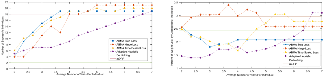
(a) Comparison of different program design methods with respect to number of successful individuals (i.e., lost 5% or more body weight)

(b) Comparison of different program design methods with respect to the percent weight lost by unsuccessful individuals (i.e., lost less than 5% body weight)

Figure 1b compares the different program designs using a secondary outcome of interest to clinicians of the average amount of weight loss of individuals who did not successfully achieve 5% weight loss. The original treatment plan of mDPP and the “do nothing” treatment plan slightly outperform the adaptive program designs at certain clinical visit budgets. This effect however is mainly due to these static plans not identifying individuals who are on the cusp of achieving 5% weight loss but might still achieve around 3-4% weight loss, while both adaptive program designs allocate clinical visits to these individuals and ensure they reach the weight loss goal of 5% weight loss. Restated, the lower weight loss of unsuccessful individuals under the behavioral analytics treatment plans is an artifact of the improved success rate of the behavioral analytics plans in helping individuals achieve 5% weight loss. This effect is further exemplified in the region of between an average of 2.8-4.2 visits per individual, where individuals who were not successful in achieving 5% weight loss in the behavioral analytics treatment plans on average lose more weight then those under the heuristic policy, while in the region of an average of 5.6-7 visits per individual individuals under the heuristic treatment lose more weight. The effect in this last region is due to the behavioral model used in our behavioral analytics framework, which is more effective at identifying the individuals who would most benefit from additional clinical visits. Therefore, more resources are spent on individuals who could potentially reach their 5% weight loss goal, while the adaptive heuristic uses these resources less effectively.

Figures 1a and 1b demonstrate a tradeoff between the primary and secondary outcomes, and how it differs between loss functions. Note the line for the step loss (25) is the first to achieve a primary outcome comparable to that of the original mDPP trial while fluctuating relatively little in terms of the secondary outcome. This matches intuition that the step loss function (25) is focused on ensuring individuals achieve 5% weight loss while not being concerned with their final weight. On the other hand, the line for the hinge loss (26) lags behind the other behavioral analytics policies in achieving comparable primary outcomes to the mDPP trial while having an effective secondary outcome. These results follow our intuition that this loss favors intermediate weight loss over achieving clinically significant weight loss. Finally, the line corresponding to the time-varying hinge loss function (27) has a transition at an average of 5 visits per individual from favoring the primary outcome to the secondary outcome. This indicates that using time scaling leads to interventions that focus on primary outcomes when resources are constrained but also accounts for secondary outcomes when resources are less scarce. Such behavior may be useful for implementing a behavioral analytics approach when the relative abundance of resources is not known a priori.

5.5. Discussion and Policy Insights

From our experimental results, it is clear that ABMA and the behavioral analytics framework provide several key insights to policy makers both in the context of personalized healthcare and more generally.

1. Personalized models allow for more efficient use of budgets. In the context of weight loss interventions, by using an ABMA approach we can achieve comparable results to the naive current clinical practice with at most 60% of the resource budget. Since the naive approach is also adaptive, it is clear that using a personalized model that can effectively estimate and compute individual policies ensures that resources are only allocated to the participants who would most benefit from them. While not examined in our experiments here, the effectiveness of an approach similar to ABMA has been shown to have potential in effecting energy consumption behavior in the context of HVAC systems (Mintz et al., 2018; Cabrera et al., 2018). This indicates that in contexts driven by individual decision making, personalized models can lead to more effective budget allocation.

2. An ABMA based approach is robust to missing data. One of the chief implementation challenges for personalized models is noisy and missing data. By using insights from the behavioral modeling literature, the predictive modeling in ABMA is able to predict the response of individuals to the policy set by the policy maker even in the presence of these data challenges. While other adaptive approaches exist that are less restrictive with their modeling assumptions, such as model free approaches (Osband & Roy, 2015; Osband et al., 2016), they tend to work poorly in environments such as those described in Section 1.1 since they either rely to heavily on data imputation of missing values causing them to over fit, or must compensate by requiring a large number of trajectories (or access to a simulator) in order to converge to a policy. Thus, an approach like ABMA, despite making stronger assumptions, leverages results from the existing literature to provide effective policies in these environments. Moreover, recent RCT’s have shown the effectiveness of ABMA with real human subjects in the context of physical activity interventions (Zhou et al., 2018b).

3. The structure of the behavioral analytics framework lends itself to parallelization and easy computation, making it viable for high risk decision making. Appendix E shows that the average run-time for our ABMA based approaches in the context of our simulation studies is approximately 17 seconds per patient for computing the candidate interventions and 13 seconds per patient for estimating their individual parameters, indicating that solving these problems at the level of the individual should only take a moderate amount of time, while the aggregate knapsack problem on average took 0.19 seconds to solve. While different applications with different formulations may deviate from these times, by decomposing the problem to individual level problems and using parallelization, these benchmarking results indicate the decomposition scheme makes ABMA an effective framework to be used for decision making at scale. Moreover, Appendix A.1 indicates that ABMA is capable of achieving effective outcomes while adapting decisions less frequently. This would again help with implementing these policies at scale since candidate interventions for larger number of participants may take more computational time, but can still be deployed effectively.

6. Conclusion

In this paper, we develop a behavioral analytics framework for multi-agent systems in which a single coordinator provides behavioral or financial incentives to a large number of myopic agents. Our framework is applicable in a variety of settings of interest to the operations research community, including the design of demand-response programs for electricity consumes and the personalized design of a weight loss program. The framework we develop involves the definition of a behavioral model, the estimation of model parameters, and the optimization of incentives. We show (among other results) that under mild assumptions, the incentives computed by our approach converge to the optimal incentives that would be computed knowing full information about the agents. We evaluated our approach for personalizing the design of a weight loss program, and showed via simulation that our approach can improve outcomes with reduced treatment cost.

Highlights.

• Adaptive and personalized incentives effective in influencing agent behavior

• Using a behavioral model based reinforcement learning, decision makers can implement asymptotically optimal interventions

• Personalized behavioral interventions more effective in helping weight loss trial participants then one size fits all

• A decomposition approach is proposed and shown to be optimal for solving bi-level optimization problems

Appendix A. Proofs of Propositions

Proof. Proof of Proposition 1: The constraints θ_t+1 = g(x_t, u_t, θ_t, π_t) can be reformulated using Assumption 3 as

$$\begin{gathered} {\theta }_{t+1}\le G_i·\left(x_t;u_t;{\theta }_t;{\pi }_t\right)+{\xi }_i+\left(1-{\iota }_i\right)·M \\ {\theta }_{t+1}\ge G_i·\left(x_t;u_t;{\theta }_t;{\pi }_t\right)+{\xi }_i-\left(1-{\iota }_i\right)·M \\ {B}_i·\left(x_t;u_t;{\theta }_t;{\pi }_t\right)\le {\psi }_i+\left(1-{\iota }_i\right)·M \\ {\iota }_i\in \{0,1\} \end{gathered}$$ (A.1)

where M > 0 is a large-enough constant. Such a finite M exists because 𝒳, 𝒰, Π, Θ, 𝒞 are compact. Hence it suffices to show u_t ∈ argmax{f(x_t+1, u, θ_t, π_t) | x_t+1 = h(x_t, u), u ∈ 𝒰} can be represented (by its optimality condition) using a finite number of mixed integer linear constraints. Suppose 𝒰 = {u: Ξu ≤ κ}, where Ξ is a matrix and κ is a vector. Recall Assumption 2

$$f(x,u,\theta ,\pi )=-{(x;u)}^T·Q·(x;u)+{(\theta ;\pi )}^T·H·(x;u)+\sum _{i=1}^K\underset{j\in J_i}{\min }\left\{F_{i,j}·(x;u;\theta ;\pi )+{\zeta }_{i,j}\right\}.$$ (A.2)

We cannot characterize optimality by differentiating f because it is generally not differentiable, but we can reformulate the maximization of (A.2) as the following convex quadratic program:

$$\begin{gathered} u_t\in \mathrm{arg\; max}-{\left(x_{t+1};u\right)}^T·Q·\left(x_{t+1};u\right)+{\left({\theta }_t;{\pi }_t\right)}^T·H·\left(x_{t+1};u\right)+\sum _{i=1}^K{w}_i \\ \text{s.t.}{w}_i\le F_{i,j}·\left(x_{t+1};u;{\theta }_t;{\pi }_t\right)+{\zeta }_{i,j}\text{for all}i,j \\ \text{Ξ}u\le \kappa \end{gathered}$$ (A.3)

Using Assumption 4, we can rewrite the above as

$$\begin{gathered} u_t\in \mathrm{arg\; max}-u^T·{\left(B;\mathbb{\text{I}}\right)}^T·Q·\left(B;\mathbb{\text{I}}\right)·u+\left({\left({\theta }_t;{\pi }_t\right)}^{T}H-2{\left(A{x}_t+k;0\right)}^{T}Q\right)·\left(B;\mathbb{I}\right)·u+\sum _{i=1}^K{w}_i \\ \text{s.t.}{w}_i\le F_{i,j}·\left(B;\mathbb{\text{I}};0;0\right)·u+F_{i,j}·\left(A{x}_t+k;0;{\theta }_t;{\pi }_t\right)+{\zeta }_{i,j}\text{for all}i,j \\ \text{Ξ}u\le \kappa \end{gathered}$$ (A.4)

where we have eliminated the constant (θ_t; π_t)^T · H · (Ax_t + k; 0) since x_t, θ_t, π_t are known to the agent. The above optimization problem is convex with a strictly concave objective function by assumption, and all constraints are linear for fixed π_t. Hence the optimality conditions for (A.4) can be characterized using the KKT conditions (Dempe, 2002; Boyd & Vandenberghe, 2004). Let λ_i,j and μ be the Lagrange Multipliers for the first and second set of constraints given in (A.4), and note the KKT conditions are

$$\begin{gathered} 2{\left(B;\mathbb{\text{I}}\right)}^T·Q·\left(B;\mathbb{\text{I}}\right)·u+{\left(B;\mathbb{\text{I}}\right)}^T·\left(2Q·\left(A{x}_t+k;0\right)-H^T·\left({\theta }_t;{\pi }_t\right)\right)+{\text{Ξ}}^T·\mu =\sum _{i=1}^K\sum _{j\in J_i}{\lambda }_{i,j}·{\left(B;\mathbb{\text{I}};0;0\right)}^T·F_{i,j}^T \\ \underset{j\in J_i}{\Sigma }{\lambda }_{i,j}=1\text{for}i=1,\dots ,K \\ {\lambda }_{i,j}·\left(w_i-F_{i,j}·\left(B;\mathbb{\text{I}};0;0\right)·u+F_{i,j}·\left(A{x}_t+k;0;{\theta }_t;{\pi }_t\right)+{\zeta }_{i,j}\right)=0\text{for all}i,j \\ {w}_i\le F_{i,j}·\left(B;\mathbb{\text{I}};0;0\right)·u+F_{i,j}·\left(A{x}_t+k;0;{\theta }_t;{\pi }_t\right)+{\zeta }_{i,j}\text{for all}i,j \\ \text{Ξ}u\le \kappa \text{and}{\lambda }_{i,j}\ge 0\text{for all}i,j \end{gathered}$$ (A.5)

Note that the only nonlinear conditions are those which represent complimentary slackness. However, these conditions can be reformulated as integer linear conditions by posing them as disjunctive constraints (Wolsey & Nemhauser, 1999): For sufficiently large M - which exists because of the compactness of 𝒳, 𝒰, Π, Θ – the complimentary slackness conditions are

$$\begin{gathered} {\lambda }_{i,j}\le M{\iota }_{i,j}\text{for all}i,j \\ {F}_{i,j}·(B;\mathbb{I};0;0)·u+F_{i,j}·\left(A{x}_t+k;0;{\theta }_t;{\pi }_t\right)+{\zeta }_{i,j}\le w_i+M·\left(1-{\iota }_{i,j}\right)\text{for all}i,j \\ {\iota }_{i,j}\in \{0,1\}\text{for all}i,j \end{gathered}$$ (A.6)

This shows that feasible region of (7) of can be represented using a finite number of mixed integer linear constraints. □

Proof. Proof of Proposition 2: Let $\left(x_T^{*},{\theta }_T^{*}\right)$ be the agent’s true current states, and observe that

$$\begin{gathered} \log \widehat{p}\left(x_T,{\theta }_T|{\left\{{\tilde{x}}_{t_i}\right\}}_{i=0}^{n_x},{\left\{{\tilde{y}}_{{\tau }_i}\right\}}_{i=0}^{n_u},{\left\{{\pi }_i\right\}}_{i=0}^{T-1}\right)=\log \widehat{p}\left(x_T^{\ast },{\theta }_T^{\ast }|{\left\{{\tilde{x}}_{t_i}\right\}}_{i=0}^{n_x},{\left\{{\tilde{y}}_{{\tau }_i}\right\}}_{i=0}^{n_u},{\left\{{\pi }_i\right\}}_{i=0}^{T-1}\right)+ \\ \sum _{i=0}^{n_x}\log \frac{p_{\nu }\left({\tilde{x}}_{t_i}-D{\overline{x}}_{t_i}\right)}{p_{\nu }\left({\tilde{x}}_{t_i}-D{x}_{t_i}^{\ast }\right)}+\sum _{j=0}^{n_n}\log \frac{p_{\omega }\left({\tilde{y}}_{{\tau }_j}-C{\overline{u}}_{{\tau }_j}\right)}{p_{\omega }\left({\tilde{y}}_{{\tau }_j}-C{u}_{{\tau }_j}^{\ast }\right)}+\log \frac{p\left({\overline{x}}_0,{\overline{\theta }}_0\right)}{p\left(x_0^{\ast },{\theta }_0^{\ast }\right)}, \end{gathered}$$ (A.7)

where $x_t^{*}$, $u_t^{*}$; are the true states and decisions, and ${\overline{x}}_t$, ${\overline{u}}_t$ are the maximizing states and decisions when solving (9). But $\log \frac{p\left({\overline{x}}_0,{\overline{\theta }}_0\right)}{p\left(x_0^{*},{\theta }_0^{*}\right)}$ is a constant by assumption, and $\log \widehat{p}\left(x_T^{*},{\theta }_T^{*}|{\left\{{\tilde{x}}_{t_i}\right\}}_{i=0}^{n_x},{\left\{{\tilde{y}}_{{\tau }_i}\right\}}_{i=0}^{n_u},{\left\{{\pi }_i\right\}}_{i=0}^{T-1}\right)\le 0$ since $\widehat{p}\left(x_T,{\theta }_T|{\left\{{\tilde{x}}_{t_i}\right\}}_{i=0}^{n_x},{\left\{{\tilde{y}}_{{\tau }_i}\right\}}_{i=0}^{n_u},{\left\{{\pi }_i\right\}}_{i=0}^{T-1}\right)\in [0,1]$ by construction. So using Assumption 5 gives ${\max }_{ℰ(\delta )}\log \widehat{p}\left(x_T,{\theta }_T|{\left\{{\tilde{x}}_{t_i}\right\}}_{i=0}^{n_x},{\left\{{\tilde{y}}_{{\tau }_i}\right\}}_{i=0}^{n_u},{\left\{{\pi }_i\right\}}_{i=0}^{T-1}\right)\to -\infty$ for any δ > 0 almost surely. Equivalently, ${\max }_{ℰ(\delta )}\widehat{p}\left(x_T,{\theta }_T|{\left\{{\tilde{x}}_{t_i}\right\}}_{i=0}^{n_x},{\left\{{\tilde{y}}_{{\tau }_i}\right\}}_{i=0}^{n_u},{\left\{{\pi }_i\right\}}_{i=0}^{T-1}\right)\to 0$ for any δ > 0 almost surely. Thus for any δ > 0 we have

$$\begin{gathered} \widehat{p}\left(ℰ(\delta )|{\left\{{\tilde{x}}_{t_i}\right\}}_{i=0}^{n_x},{\left\{{\tilde{y}}_{{\tau }_i}\right\}}_{i=0}^{n_u},{\left\{{\pi }_i\right\}}_{i=0}^{T-1}\right)={\int }_{ℰ(\delta )}\widehat{p}\left(x_T,{\theta }_T\mid {\left\{{\tilde{x}}_{t_i}\right\}}_{i=0}^{n_x},{\left\{{\tilde{y}}_{{\tau }_i}\right\}}_{i=0}^{n_u},{\left\{{\pi }_i\right\}}_{i=0}^{T-1}\right)\times d{x}_0\times d{\theta }_0\le \\ \text{volume}(𝒳\times \text{Θ})·{\max }_{ℰ(\delta )}\widehat{p}\left(x_T,{\theta }_T|{\left\{{\tilde{x}}_{t_i}\right\}}_{i=0}^{n_x},{\left\{{\tilde{y}}_{{\tau }_i}\right\}}_{i=0}^{n_u},{\left\{{\pi }_i\right\}}_{i=0}^{T-1}\right)\to 0 \end{gathered}$$ (A.8)

almost surely. This proves the result since (A.8) holds almost surely for any δ > 0. □

Proof. Proof of Corollary 3: Consider the events $E_1=\left\{\left({\widehat{x}}_T,{\widehat{\theta }}_T\right)\notin ℬ\left(x_T^{*},{\theta }_T^{*},\delta \right)\right\}$ and $E_2=\{{\max }_{ℰ(\delta )}\widehat{p}\left(x_T,{\theta }_T|{\left\{{\tilde{x}}_{t_i}\right\}}_{i=0}^{n_x},{\left\{{\tilde{y}}_{{\tau }_l}\right\}}_{i=0}^{n_u},{\left\{{\pi }_i\right\}}_{i=0}^{T-1}\right)\ge {\max }_{\left(x_T,{\theta }_T\right)\in ℬ\left(x_T^{*},{\theta }_T^{*},\delta \right)}\widehat{p}\left(x_T,{\theta }_T|{\left\{{\tilde{x}}_{t_i}\right\}}_{i=0}^{n_x},{\left\{{\tilde{y}}_{{\tau }_i}\right\}}_{i=0}^{n_u},{\left\{{\pi }_i\right\}}_{i=0}^{T-1}\right)\}$ where ℰ(δ) is defined as before for some δ > 0. Then observe that E₁ ⊂ E₂, therefore $\mathbb{P}\left(E_1\right)\le \mathbb{P}\left(E_2\right)$. By Proposition 2 as T → ∞, $\mathbb{P}\left(E_2\right)\to 0$ hence $\mathbb{P}\left(E_1\right)\to 0$. Thus the result of the corollary follows. □

Proof. Proof of Corollary 4: For the first result, note Proposition 1 implies the feasible region of (15) can be expressed as mixed integer linear constraints with respect to (x_t, u_t, θ_t, π_t). Thus $\phi \left({\overline{x}}_T,{\overline{\theta }}_T,{\left\{{\overline{\pi }}_i\right\}}_{i=T}^{T+n-1}\right)$ is the value function of a MILP in which x_T, θ_T, ${\overline{\pi }}_t$ belong to an affine term. Standard results (Ralphs & Hassanzadeh, 2014) imply the value function is lower semicontinuous with respect to x_T, θ_T, ${\left\{{\pi }_i\right\}}_{i=T}^{T+n-1}$.

To show the second result, note that the problem of $\min \phi \left(x_T,{\theta }_T,{\left\{{\pi }_i\right\}}_{i=T}^{T+n-1}\right)$ is equivalent to (15) but with removal of the constraints ${\pi }_t={\overline{\pi }}_t$ for t = T, …, T + n − 1. And so the result follows by Proposition 1 and by recalling the assumptions on Π and ℓ. □

Proof. Proof of Proposition 3: We begin by proving the first result. Fist by definition we have that

$$\begin{gathered} \mathbb{E}\left[\phi \left(x_T,{\theta }_T,{\left\{{\pi }_i\right\}}_{i=T}^{T+n-1}\right)\mid {\left\{{\tilde{x}}_{t_i}\right\}}_{i=0}^{n_x},{\left\{{\tilde{y}}_{{\tau }_i}\right\}}_{i=0}^{n_u},{\left\{{\pi }_i\right\}}_{i=0}^{T-1}\right]= \\ {\int }_{𝒳\times \text{Θ}}\phi \left(x_T,{\theta }_T,{\left\{{\pi }_i\right\}}_{i=T}^{T+n-1}\right)p\left(x_T,{\theta }_T\mid {\left\{{\tilde{x}}_{t_i}\right\}}_{i=0}^{n_x},{\left\{{\tilde{y}}_{{\tau }_i}\right\}}_{i=0}^{n_u},{\left\{{\pi }_i\right\}}_{i=0}^{T-1}\right)\times d{x}_T\times d{\theta }_T. \end{gathered}$$ (A.9)

Now note that a nearly identical argument as in the proof of Corollary 4 gives that φ is lower semicontinuous. Then, because of Proposition 2, the result follows directly by Theorem 3.5 from (Vogel & Lachout, 2003b) and Proposition 5.1 from (Vogel & Lachout, 2003a).

For the second result, recall that Corollary 3 implies $\left({\widehat{x}}_T,{\widehat{\theta }}_T\right)\stackrel{p}{\to }\left(x_T^{*},{\theta }_T^{*}\right)$. And Corollary 4 gives that $\phi \left(x_T,{\theta }_T,{\left\{{\pi }_i\right\}}_{i=T}^{T+n-1}\right)$ is lower semicontinuous in $x_T,{\theta }_T,{\left\{{\pi }_i\right\}}_{i=T}^{T+n-1}$. The result then follows by direct application of Proposition 2.1.ii of (Vogel & Lachout, 2003b). □

Proof. Proof of Theorem 1: The result follows by combining the first and second parts of our Proposition 3 with Theorem 4.3 from (Vogel & Lachout, 2003a). □

Proof. Proof of Proposition 4: Step 2 of ABMA is a MAP estimate, which can be computed by solving a single MILP by Corollary 2. A similar argument used to prove Corollary 4 shows that Steps 4 and 5 can be computed by solving a single MILP. Step 8 can be seen to be an ILP by construction. The remaining steps of ABMA are assignment steps and do not require solving any optimization problems. □

Proof. Proof of Proposition 5: Using the assumptions on decomposibility on the incentive set Ω (Assumption 9), we have that (19) can be reformulated as

$$\begin{gathered} \underset{{\left\{{\pi }_i^a\right\}}_{i=T}^{T+n-1},{\varphi }_v^a,y_v^a,\forall v,a\in V\times 𝒜}{\min }{\sum }_{a\in 𝒜}{\sum }_{v\in V}{\varphi }_v^a·y_v^a \\ \text{s.t.}\min \left\{{\phi }^a\left(x_T^a,{\theta }_T^a,{\left\{{\pi }_i^{v,a}\right\}}_{i=T}^{T+n-1}\right)|{\left\{{\pi }_i^{v,a}\right\}}_{i=T}^{T+n-1}\in S_v\right\}\le {\varphi }_v^a \\ {\sum }_{a\in 𝒜}{\sum }_{v\in V}v·y_v^a\le \beta \\ {\sum }_{v\in V}{y}_v^a=1\text{for}a\in 𝒜 \\ {y}_v^a\in \{0,1\}\text{for}v\in V,a\in 𝒜 \\ {\overline{\pi }}_i^a={\sum }_{v\in V}{\pi }_i^{v,a}·y_v^a\text{for}a\in 𝒜,T\le i\le T+n-1 \end{gathered}$$ (A.10)

Since ${\varphi }_v^a·y_v^a$ and ${\pi }_i^{v,a}·y_v^a$ are the product of a continuous and binary decision variable, standard integer programming reformulation techniques allow us to reformulate the above as

$$\begin{gathered} \underset{{\left\{{\pi }_i^a\right\}}_{i=T}^{T+n-1},{\varphi }_v^a,z_v^a,{\left\{{\eta }_i^{v,a}\right\}}_{i=T}^{T+n-1},y_v^a,\forall v,a\in V\times 𝒜}{\min }{\sum }_{a\in 𝒜}{\sum }_{v\in V}{z}_v^a \\ \text{s.t.}{\phi }^a\left(x_T,{\theta }_T,{\left\{{\pi }_i^{v,a}\right\}}_{i=T}^{T+n-1}\right)\le {\varphi }_v^a \\ {\left\{{\pi }_i^{v,a}\right\}}_{i=T}^{T+n-1}\in S_v\text{for}a\in 𝒜 \\ {\sum }_{a\in 𝒜}{\sum }_{v\in V}v·y_v^a\le \beta \\ {\sum }_{v\in V}{y}_v^a=1\text{for}a\in 𝒜 \\ {y}_v^a\in \{0,1\}\text{for}v\in V,a\in 𝒜 \\ {\overline{\pi }}_i^a={\sum }_{v\in V}{\eta }_i^{v,a}\text{for}a\in 𝒜,T\le i\le T+n-1 \\ {z}_v^a\ge {\varphi }_v^a-M·\left(1-y_v^a\right)\text{for}v\in V,a\in 𝒜 \\ {z}_v^a\le {\varphi }_v^a+M·\left(1-y_v^a\right)\text{for}v\in V,a\in 𝒜 \\ {z}_v^a\le M·y_v^a\text{for}v\in V,a\in 𝒜 \\ {z}_v^a\ge -M·y_v^a\text{for}v\in V,a\in 𝒜 \\ {\eta }_i^{v,a}\ge {\pi }_i^{v,a}-M·\left(1-y_v^a\right)\text{for}v\in V,a\in 𝒜 \\ {\eta }_i^{v,a}\le {\pi }_i^{v,a}+M·\left(1-y_v^a\right)\text{for}v\in V,a\in 𝒜 \\ {\eta }_i^{v,a}\le M·y_v^a\text{for}v\in V,a\in 𝒜 \\ {\eta }_i^{v,a}\ge -M·y_v^a\text{for}v\in V,a\in 𝒜 \end{gathered}$$ (A.11)

where M > 0 is a large-enough constant. Such a finite M exists because 𝒳, 𝒰, Π, Θ are compact, and because ℓ^a is representable by a finite number of mixed integer linear constraints. Since Corollary 4 (and its proof) implies we can represent ${\phi }^a\left(x_T,{\theta }_T,{\left\{{\pi }_i^{v,a}\right\}}_{i=T}^{T+n-1}\right)\le {\varphi }_v^a$ and ${\left\{{\pi }_i^{v,a}\right\}}_{i=T}^{T+n-1}\in S_v$ by mixed integer linear constraints, this means we can reformulate (19) as a MILP with linear constraints that are affine in ($x_T^a,{\theta }_T^a,{\left\{{\overline{\pi }}_i^a\right\}}_{i=T}^{T+n-1}$ for a ∈ 𝒜). And so standard results (Ralphs & Hassanzadeh, 2014) imply its value function is lower semicontinuous with respect to these variables, which is our first result. The second result follows by noting min Λ($x_T^a,{\theta }_T^a,{\left\{{\overline{\pi }}_i^a\right\}}_{i=T}^{T+n-1}$ for a ∈ 𝒜) is equivalent to (19) but with removal of the constraints ${\pi }_t^a={\overline{\pi }}_t^a$ for a ∈ 𝒜 and t = T, …, T + n − 1. □

Proof. Proof of Theorem 2: First, note that a nearly identical argument to the one in the proofs of Corollary 4 and Proposition 5 gives that Λ is lower semicontinuous. Then, because of Proposition 2, we have that Λ($x_T^{*,a},{\theta }_T^{*,a},{\left\{{\pi }_i^a\right\}}_{i=T}^{T+n-1}$ for a ∈ 𝒜) is a lower semicontinuous approximation to $\mathbb{E}[\Lambda (x_T^a,{\theta }_T^a,{\left\{{\overline{\pi }}_i^a\right\}}_{i=T}^{T+n-1}$ for $𝒜))|{\left\{{\tilde{x}}_{t_i}^a\right\}}_{i=0}^{T_i^a},{\left\{{\tilde{y}}_{{\tau }_i}^a\right\}}_{i=0}^{T_u^a},{\left\{{\pi }_i^a\right\}}_{i=0}^{T-1}$ for a ∈ 𝒜] by Theorem 3.5 from (Vogel & Lachout, 2003b) and Proposition 5.1 from (Vogel & Lachout, 2003a). Next note that Corollary 3 implies $\left({\widehat{x}}_T^a,{\widehat{\theta }}_T^a\right)\stackrel{p}{\to }\left(x_T^{*,a},{\theta }_T^{*,a}\right)$, and Proposition 5 states Λ is lower semicontinuous in its arguments. This means Λ(${\widehat{x}}_T^a,{\widehat{\theta }}_T^a,{\left\{{\pi }_i^a\right\}}_{i=T}^{T+n-1}$ for a ∈ 𝒜) is a lower semicontinuous approximation to Λ($x_T^{*,a},{\theta }_T^{*,a},{\left\{{\pi }_i^a\right\}}_{i=T}^{T+n-1}$ for a ∈ 𝒜) by Proposition 2.1.ii of (Vogel & Lachout, 2003b). But Corollary 5 shows that

$$\left\{{\pi }_{ABMA}^a(T)\text{for}a\in 𝒜\right\}\in \mathrm{arg\; min}\text{Λ}\left({\widehat{x}}_T^a,{\widehat{\theta }}_T^a,{\left\{{\pi }_i^a\right\}}_{i=T}^{T+n-1}\text{for}a\in 𝒜\right)\text{.}$$ (A.12)

This means that the result follows by applying Theorem 4.3 from (Vogel & Lachout, 2003a). □

Appendix A.1. Computational Performance and Sensitivity Analysis

The experiments assumed that treatment plans were updated at the beginning of each month by rerunning the second and third steps of our behavioral analytics approach (through applying ABMA), and so we conducted a sensitivity analysis to examine the effect of updating the program design more or less frequently. Figures A.2 and A.3 compare the health outcomes of using a program designed by our behavioral analytics framework with a time-varying hinge loss (27), where the treatment was recalculated once every two weeks, once a month, and once every two months. These results show that recomputing the treatment plan with lesser or higher frequency does not significantly impact the efficacy of the resulting treatment. This indicates that for practical implementation, the statistical convergence rate of estimated parameters in our behavioral model is sufficiently fast that it would suffice to rerun the algorithm at most once a month.

We also conducted time-benchmarks for the sub-problems involved in computing 2SSA, MAP, and ABMA, which are the algorithms comprising the second and third steps of our implementation o a behavioral analytics framework. The results of the time-benchmarks are summarized in Tables E.1, E.2, and E.3 in the appendix. On average, solving all sub-problems took 17s per individual. This is promising for practical implementation, particularly because each sub-problem calculation can be performed in parallel for each size constraint of the clinical visit schedule (from 1 to 7 visits). The results show that computation time increases with respect to the number of available visits and data available in the treatment plan calculation. However, the calculation times still remain below 30s on average per individual for each step of the program calculation. This would imply that our methodology for weight loss program calculation is suitable for large scale program design since the program design would be updated at most once every month.

Figure A.2:

Comparison of calculation schedules and their effects on the number of successful individuals (i.e., lost 5% or more body weight)

Figure A.3:

Comparison of calculation schedules and their effects on the weight lost by unsuccessful individuals (i.e., lost less than 5% body weight)

Appendix B. Complete MILP Formulation of MLE Problem

$$\min \frac{\sqrt{2}}{{\sigma }_1}\sum _{i=1}^{n_w}{\zeta }_{w,t_i}+\frac{\sqrt{2}}{{\sigma }_2}\sum _{i=1}^{n_s}{\zeta }_{s,t_i}$$ (B.1)

$$\text{s.t.}-{\zeta }_{w,t_i}\le {\tilde{w}}_{t_i}-w_{t_i}\le {\zeta }_{w,t_i}\forall 1\le t_i\le n_w$$ (B.2)

$$-{\zeta }_{s,t_i}\le {\tilde{s}}_{{\tau }_i}-s_{{\tau }_i}\le {\zeta }_{s,t_i}\forall 1\le t_i\le n_s$$ (B.3)

$$-b\left(a{w}_1+b{s}_0+c{f}_0+k\right)-r_s\left(s_0-s_b\right)=0$$ (B.4)

$$-\left(a{w}_1+b{s}_0+c{f}_0+k\right)-r_f\left(f_0-F_{b,1}\right)=0$$ (B.5)

$$-b\left(a{w}_t+b{s}_t+c{f}_t+k\right)-r_s\left(s_t-s_b\right)=0\forall 1\le t\le m$$ (B.6)

$$-\left(a{w}_t+b{s}_t+c{f}_t+k\right)-r_f\left(f_t-f_{b,t}\right)=0\forall 1\le t\le m$$ (B.7)

$$-2b\left(a{w}_t+b{s}_t+c{f}_t+k\right)-2r_s\left(s_t-s_b\right)+{\lambda }_{1,t}=0\forall m\le t\le n$$ (B.8)

$$-2\left(a{w}_t+b{s}_t+c{f}_t+k\right)-2\left(f_t-f_{b,t}\right)=0\forall m\le t\le n$$ (B.9)

$$\left(g_t-ϵ\right)-M{x}_{1,t}\le s_t\le g_t-ϵ+M\left(1-x_{1,t}\right)\forall m\le t\le n$$ (B.10)

$$\left(g_t-ϵ\right)-M\left(1-x_{2,t}\right)\le s_t\le g_t+ϵ+M\left(1-x_{2,t}\right)\forall m\le t\le n$$ (B.11)

$$\left(g_t+ϵ\right)-M\left(1-x_{3,t}\right)\le s_t\le g_t+ϵ+M{x}_{3,t}\forall m\le t\le n$$ (B.12)

$$p_t-M\left(1-x_{t,1}\right)\le {\lambda }_{1,t}\le M\left(1-x_{3,t}\right)\forall m\le t\le n$$ (B.13)

$$0\le {\lambda }_{1,t}\le p_t\forall m\le t\le n$$ (B.14)

$$x_{t,1}+x_{t,2}+x_{t,3}=1\forall m\le t\le n$$ (B.15)

$$p_{t+1}\ge \gamma p_t+\delta d_{t+1}\forall m\le t\le n$$ (B.16)

$$p_{t+1}\le \gamma p_t+\delta d_{t+1}+M\left(1-x_{1,t}\right)\forall m\le t\le n$$ (B.17)

$$p_{t+1}\ge \gamma p_t+\delta d_{t+1}+\mu -M{x}_{1,t}\forall m\le t\le n$$ (B.18)

$$p_{t+1}\le \gamma p_t+\delta d_{t+1}+\mu \forall m\le t\le n$$ (B.19)

$$F_{b,t+1}=(1-\alpha )F_{b,t}+\alpha f_{b,t}\forall t$$ (B.20)

$$f_{b,t+1}=\gamma \left(f_{b,t}-F_{b,t}\right)+F_{b,t}-\beta d_t\forall t$$ (B.21)

$$x_{t+1,1}\ge x_{t,1}-d_{t+1}-\mathbb{1}\left(g_{t+1}-g_t<0\right)\forall m\le t\le n$$ (B.22)

$$x_{t+1,2}\le x_{t,2}-d_{t+1}+\mathbb{1}\left(g_{t+1}-g_t<0\right)\forall m\le t\le n$$ (B.23)

$$x_{t+1,3}\le x_{t,3}-d_{t+1}+\mathbb{1}\left(g_{t+1}-g_t<0\right)\forall m\le t\le n$$ (B.24)

$$w_t,s_t,f_t,F_{b,t},f_{b,t},p_t\ge 0\forall t$$ (B.25)

$$x_{t,1},x_{t,2},x_{t,3}\in \mathbb{B}\forall t$$ (B.26)

Appendix C. Complete MILP Formulation of MAP Problem

$$\min \frac{\sqrt{2}}{{\sigma }_1}\sum _{i=1}^{n_w}{\zeta }_{w,t_i}+\frac{\sqrt{2}}{{\sigma }_2}\sum _{i=1}^{n_s}{\zeta }_{s,t_i}-\sum _{x\in \theta }\sum _{i=1}^{m_x}{z}_{i,x}\log {\varphi }_i^x$$ (C.1)

$$\text{s.t.}-{\zeta }_{w,t_i}\le {\tilde{w}}_{t_i}-w_{t_i}\le {\zeta }_{w,t_i}\forall 1\le t_i\le n_w$$ (C.2)

$$-{\zeta }_{s,t_i}\le {\tilde{s}}_{{\tau }_i}-s_{{\tau }_i}\le {\zeta }_{s,t_i}\forall 1\le t_i\le n_s$$ (C.3)

$$-b\left(a{w}_1+b{s}_0+c{f}_0+k\right)-r_s\left(s_0-s_b\right)=0$$ (C.4)

$$-\left(a{w}_1+b{s}_0+c{f}_0+k\right)-r_f\left(f_0-F_{b,1}\right)=0$$ (C.5)

$$-b\left(a{w}_t+b{s}_t+c{f}_t+k\right)-r_s\left(s_t-s_b\right)=0\forall 1\le t\le m$$ (C.6)

$$-\left(a{w}_t+b{s}_t+c{f}_t+k\right)-r_f\left(f_t-f_{b,t}\right)=0\forall 1\le t\le m$$ (C.7)

$$-2b\left(a{w}_t+b{s}_t+c{f}_t+k\right)-2r_s\left(s_t-s_b\right)+{\lambda }_{1,t}=0\forall m\le t\le n$$ (C.8)

$$-2\left(a{w}_t+b{s}_t+c{f}_t+k\right)-2\left(f_t-f_{b,t}\right)=0\forall m\le t\le n$$ (C.9)

$$\left(g_t-ϵ\right)-M{x}_{1,t}\le s_t\le g_t-ϵ+M\left(1-x_{1,t}\right)\forall m\le t\le n$$ (C.10)

$$\left(g_t-ϵ\right)-M\left(1-x_{2,t}\right)\le s_t\le g_t+ϵ+M\left(1-x_{2,t}\right)\forall m\le t\le n$$ (C.11)

$$\left(g_t+ϵ\right)-M\left(1-x_{3,t}\right)\le s_t\le g_t+ϵ+M{x}_{3,t}\forall m\le t\le n$$ (C.12)

$$p_t-M\left(1-x_{t,1}\right)\le {\lambda }_{1,t}\le M\left(1-x_{3,t}\right)\forall m\le t\le n$$ (C.13)

$$0\le {\lambda }_{1,t}\le p_t\forall m\le t\le n$$ (C.14)

$$x_{t,1}+x_{t,2}+x_{t,3}=1\forall m\le t\le n$$ (C.15)

$$p_{t+1}\ge \gamma p_t+\delta d_{t+1}\forall m\le t\le n$$ (C.16)

$$p_{t+1}\le \gamma p_t+\delta d_{t+1}+M\left(1-x_{1,t}\right)\forall m\le t\le n$$ (C.17)

$$p_{t+1}\ge \gamma p_t+\delta d_{t+1}+\mu -M{x}_{1,t}\forall m\le t\le n$$ (C.18)

$$p_{t+1}\ge \gamma p_t+\delta d_{t+1}+\mu \forall m\le t\le n$$ (C.19)

$$F_{b,t+1}=(1-\alpha )F_{b,t}+\alpha f_{b,t}\forall t$$ (C.20)

$$f_{b,t+1}=\gamma \left(f_{b,t}-F_{b,t}\right)+F_{b,t}-\beta d_t\forall t$$ (C.21)

$$x_{t+1,1}\ge x_{t,1}-d_{t+1}-\mathbb{1}\left(g_{t+1}-g_t<0\right)\forall m\le t\le n$$ (C.22)

$$x_{t+1,2}\le x_{t,2}-d_{t+1}+\mathbb{1}\left(g_{t+1}-g_t<0\right)\forall m\le t\le n$$ (C.23)

$$x_{t+1,3}\le x_{t,3}-d_{t+1}+\mathbb{1}\left(g_{t+1}-g_t<0\right)\forall m\le t\le n$$ (C.24)

$$z_{i,x}{h}_{lb,i}^x\le x_i\le z_{i,x}{h}_{ub,i}^x\forall x\forall i$$ (C.25)

$$\sum _{i=1}^{m_x}{z}_{i,x}=1\forall x\forall i$$ (C.26)

$$\sum _{i=1}^{m_x}{x}_i=x\forall x\forall i$$ (C.27)

$$z_{i,x}\in \mathbb{B}\forall x\forall i$$ (C.28)

$$w_t,s_t,f_t,F_{b,t},f_{b,t},p_t\ge 0\forall t$$ (C.29)

$$x_{t,1},x_{t,2},x_{t,3}\in \mathbb{B}\forall t$$ (C.30)

Appendix D. Complete MILP Formulation of Personalized Treatment Plan Design Problem

$$\min w_n$$ (D.1)

$$\text{s.t.}{F}_{b,t+1}=(1-\alpha )F_{b,t}+\alpha f_{b,t}\forall t>T$$ (D.2)

$$f_{b,t+1}=\gamma \left(f_{b,t}-F_{b,t}\right)+F_{b,t}-\widehat{\beta }{d}_t\forall t>T$$ (D.3)

$$p_{t+1}=\gamma p_t+\widehat{\delta }{d}_t+\widehat{\mu }\left(1-x_{1,t}\right)\forall t>T$$ (D.4)

$$d_t\le \mathbb{1}[\mathrm{mod}(t,7)=1]\forall t>T$$ (D.5)

$$d_t\le 1-d_{\tau }\forall \tau >T,\tau +1\le t\le \tau +6\forall t>T$$ (D.6)

$$-2b\left(a{w}_t+b{s}_t+c{f}_t+k\right)-2r_s\left(s_t-s_b\right)+{\lambda }_{1,t}+{\lambda }_{4,t}=0\forall t>T$$ (D.7)

$$-2\left(a{w}_t+b{s}_t+c{f}_t+k\right)-2\left(f_t-f_{b,t}\right)+{\lambda }_{3,t}=0\forall t>T$$ (D.8)

$$\left(g_t-ϵ\right)-M{x}_{1,t}\le s_t\le g_t-ϵ+M\left(1-x_{1,t}\right)\forall t>T$$ (D.9)

$$\left(g_t-ϵ\right)-M\left(1-x_{2,t}\right)\le s_t\le g_t+ϵ+M\left(1-x_{2,t}\right)\forall t>T$$ (D.10)

$$\left(g_t+ϵ\right)-M\left(1-x_{3,t}\right)\le s_t\le g_t+ϵ+M{x}_{3,t}\forall t>T$$ (D.11)

$$p_t-M\left(1-x_{t,1}\right)\le {\lambda }_{1,t}\le M\left(1-x_{3,t}\right)\forall t>T$$ (D.12)

$$0\le f_t\le M\left(1-x_{f,t}\right)\forall t>T$$ (D.13)

$$0\le s_t\le M\left(1-x_{s,t}\right)\forall t>T$$ (D.14)

$$0\le {\lambda }_{3,t}\le M{x}_{f,t}\forall t>T$$ (D.15)

$$0\le {\lambda }_{4,t}\le M{x}_{s,t}\forall t>T$$ (D.16)

$$0\le {\lambda }_{1,t}\le p_t\forall t>T$$ (D.17)

$$x_{t,1}+x_{t,2}+x_{t,3}=1\forall t>T$$ (D.18)

$$g_{t+1}-g_t\le M\left(1-g_{ind,t}\right)\forall t>T$$ (D.19)

$$g_{t+1}-g_t\ge -M{g}_{ind,t}\forall t>T$$ (D.20)

$$x_{t+1,1}\ge x_{t,1}-d_{t+1}-g_{ind,t}\forall t>T$$ (D.21)

$$x_{t+1,2}\le x_{t,2}-d_{t+1}+g_{ind,t}\forall t>T$$ (D.22)

$$x_{t+1,3}\le x_{t,3}-d_{t+1}+g_{ind,t}\forall t>T$$ (D.23)

$$g_{ind,t}\in \mathbb{B}$$ (D.24)

$$x_{t,1},x_{t,2},x_{t,3},x_{f,t},x_{s,t}\in \mathbb{B}$$ (D.25)

$$d_t={\overline{d}}_t;g_t={\overline{g}}_t;w_t={\widehat{w}}_t;s_t={\widehat{s}}_t;f_t={\widehat{f}}_t;{\theta }_t={\widehat{\theta }}_t\forall t\le T$$ (D.26)

Appendix E. Benchmarking Performance Tables

Table E.1.

Average Runtimes for Candidate Treatment Plan Calculation (in seconds)
		Date of Calculation During the Program
		15	30	60	90	120	Average
	54	21.715	9.3363	8.8984	9.5618	10.003	11.903
	63	21.715	7.7624	14.714	18.736	16.692	15.924
	72	21.715	8.8894	21.239	26.186	16.091	18.824
	81	21.715	11.408	43.147	28.112	23.284	25.533
	90	21.715	10.274	23.935	13.421	33.6	20.589
	99	21.715	9.3366	26.251	14.16	19.855	18.263
	108	21.715	9.4194	24.208	12.774	21.757	17.975
	117	21.715	9.9031	22.962	9.9226	31.865	19.273
Visit Budget	126	21.715	10.217	21.749	10.199	28.664	18.509
	135	21.715	9.973	16.307	23.129	18.893	18.003
	144	21.715	11.208	14.626	14.851	8.9203	14.264
	153	21.715	12.978	13.913	13.892	8.0501	14.11
	162	21.715	12.403	14.674	14.434	10.965	14.838
	171	21.715	13.305	12.102	11.585	23.78	16.497
	180	21.715	14.879	12.116	11.964	18.473	15.829
	189	21.715	11.731	11.835	12.221	21.715	15.843
	Average	21.715	10.814	18.917	15.322	19.538	17.261

Table E.2.

Average Runtimes for MAP Calculation (in seconds)
		Data of Calculation During the Program
		15	30	60	90	120	Average
	54	16.365	11.416	9.537	11.479	7.6851	11.296
	63	16.365	13.249	12.816	17.157	11.493	14.216
	72	16.365	11.913	14.15	13.846	12.884	13.832
	81	16.365	17.448	16.11	11.936	17.237	15.819
	90	16.365	12.251	9.9218	8.9877	16.463	12.798
	99	16.365	9.9473	10.59	9.3482	13.666	11.983
	108	16.365	10.412	10.199	9.377	14.746	12.22
	117	16.365	10.696	9.5879	8.9027	23.187	13.748
Visit Budget	126	16.365	10.36	10.737	9.6123	23.524	14.12
	135	16.365	9.7085	10.241	12.753	18.221	13.458
	144	16.365	9.3022	13.258	12.135	11.654	12.543
	153	16.365	8.5183	11.297	11.527	11.152	11.772
	162	16.365	9.4638	8.4174	11.279	14.812	12.068
	171	16.365	8.0878	11.092	9.8865	18.003	12.687
	180	16.365	8.8929	7.5454	6.5939	12.739	10.427
	189	16.365	7.679	7.6401	6.9321	16.365	10.996
	Average	16.365	10.584	10.821	10.735	15.239	12.749

Table E.3.

Average Runtimes for Knapsack Calculation (in seconds)
		Date of Calculation During the Program
		15	30	60	90	120	Average
	54	0.21791	0.19278	0.14949	0.1666	0.19679	0.18471
	63	0.19295	0.16084	0.19613	0.23577	0.22246	0.20163
	72	0.21302	0.2516	0.17474	0.18052	0.3125	0.22648
	81	0.25345	0.3542	0.18128	0.17449	0.25997	0.24468
	90	0.21698	0.17154	0.168	0.16942	0.21394	0.18798
	99	0.17072	0.17607	0.15058	0.15699	0.20012	0.1709
	108	0.17086	0.17178	0.17235	0.15172	0.19029	0.1714
	117	0.17958	0.17073	0.16465	0.16171	0.20232	0.1758
Visit Budget	126	0.18599	0.24335	0.17326	0.16726	0.20706	0.19538
	135	0.20403	0.16143	0.16626	0.16681	0.19607	0.17892
	144	0.17733	0.14174	0.16112	0.1618	0.18708	0.16581
	153	0.18841	0.15411	0.17753	0.17965	0.18822	0.17758
	162	0.17892	0.2167	0.18539	0.17419	0.21756	0.19455
	171	0.1771	0.29787	0.21357	0.2248	0.21789	0.22625
	180	0.20535	0.18508	0.22285	0.16565	0.19392	0.19457
	189	0.18554	0.2104	0.19875	0.17776	0.20053	0.1946
	Average	0.19488	0.20376	0.1785	0.17595	0.21292	0.1932

References

- Adlakha S, & Johari R (2013). Mean field equilibrium in dynamic games with strategic complementarities. OR, 61, 971–989. [Google Scholar]
- Ahuja R, & Orlin J (2001). Inverse optimization. OR, 49, 771–783. [Google Scholar]
- Astrom K, & Wittenmark B (1995). Adaptive Control. Addison–Wesley. [Google Scholar]
- Aswani A (2019). Statistics with set-valued functions: applications to inverse approximate optimization. Mathematical Programming, 174, 225–251. [Google Scholar]
- Aswani A, Gonzalez H, Sastry S, & Tomlin C (2013). Provably safe and robust learning-based model predictive control. Automatica, 49, 1216–1226. [Google Scholar]
- Aswani A, Kaminsky P, Mintz Y, Flowers E, & Fukuoka Y (2019). Behavioral modeling in weight loss interventions. EJOR, 272, 1058–1072. Available at SSRN: https://ssrn.com/abstract=2838443. [DOI] [PMC free article] [PubMed] [Google Scholar]
- Aswani A, Shen Z-J, & Siddiq A (2018). Inverse optimization with noisy data. OR, 66, 870–892. [Google Scholar]
- Aswani A, & Tomlin C (2009). Monotone piecewise affine systems. IEEE TAC, 54, 1913–1918. [Google Scholar]
- Ayer T, Alagoz O, & Stout N (2012). A POMDP approach to personalize mammography screening decisions. OR, 60, 1019–1034. [Google Scholar]
- Ayer T, Alagoz O, Stout N, & Burnside E (2015). Heterogeneity in women’s adherence and its role on optimal breast cancer screening policies. MS, . [Google Scholar]
- Ban G, & Rudin C (2016). The big data newsvendor: Practical insights from machine learning.
- Bandura A (1998). Health promotion from the perspective of social cognitive theory. Psychology and Health, 13, 623–649. [Google Scholar]
- Bastani H, & Bayati M (2015). Online decision-making with high-dimensional covariates. Available at SSRN 2661896, . [Google Scholar]
- Bertsimas D, & Goyal V (2012). On the power and limitations of affine policies in two-stage adaptive optimization. Mathematical programming, 134, 491–531. [Google Scholar]
- Bertsimas D, Gupta V, & Paschalidis I (2014). Data-driven estimation in equilibrium using inverse optimization. Mathematical Programming, (pp. 1–39). [Google Scholar]
- Bertsimas D, & O’Hair A (2013). Personalized diabetes management: A robust optimization approach. Submitted.
- Bickel P, & Doksum K (2006). Mathematical Statistics: Basic Ideas And Selected Topics volume 1. (2nd ed.). Pearson Prentice Hall. [Google Scholar]
- Bitmead R (1984). Persistence of excitation conditions and the convergence of adaptive schemes. IEEE Transactions on Information Theory, 30, 183–191. [Google Scholar]
- Blanchet J, Gallego G, & Goyal V (2013). A markov chain approximation to choice modeling. In EC (pp. 103–104). Citeseer. [Google Scholar]
- Boukhtouta A, Berger J, Powell W, & George A (2011). An adaptive-learning framework for semi-cooperative multi-agent coordination. In ADPRL (pp. 324–331). IEEE. [Google Scholar]
- Boyd S, & Vandenberghe L (2004). Convex Optimization. Cambridge University Press. [Google Scholar]
- Breiman L et al. (2001). Statistical modeling: The two cultures (with comments and a rejoinder by the author). Statistical Science, 16, 199–231. [Google Scholar]
- Brock D, & Wartman S (1990). When competent patients make irrational choices. NEJM, 322, 1595–1599. [DOI] [PubMed] [Google Scholar]
- Cabrera JA, Mintz Y, Pedrasa JR, & Aswani A (2018). Designing real-time prices to reduce load variability with hvac. In 2018 Annual American Control Conference (ACC) (pp. 6170–6175). IEEE. [Google Scholar]
- Callier F, & Desoer C (1994). Linear System Theory. Springer Texts in Electrical Engineering. Springer New York. [Google Scholar]
- Cawley J (2004). An economic framework for understanding physical activity and eating behaviors. AJPM, 27, 117–125. [DOI] [PubMed] [Google Scholar]
- Chapman G, & Elstein A (1995). Valuing the future: temporal discounting of health and money. Medical Decision Making, 15, 373–386. [DOI] [PubMed] [Google Scholar]
- Conner M, & Norman P (1996). Predicting health behaviour: research and practice with social cognition models. Open University Press. [Google Scholar]
- Costa L, & Kariniotakis G (2007). A stochastic dynamic programming model for optimal use of local energy resources in a market environment. In Power Tech, 2007 IEEE Lausanne (pp. 449–454). IEEE. [Google Scholar]
- Craig J, Hsu P, & Sastry S (1987). Adaptive control of mechanical manipulators. The International Journal of Robotics Research, 6, 16–28. [Google Scholar]
- Darby S (2010). Smart metering: What potential for householder engagement? Building Research and Information, 38, 442–457. [Google Scholar]
- Dempe S (2002). Foundations of Bilevel Programming. Springer. [Google Scholar]
- DeNegre S, & Ralphs T (2009). A branch-and-cut algorithm for bilevel integer programming. In Proceedings of the Eleventh INFORMS Computing Society Meeting (pp. 65–78). [Google Scholar]
- Deng R, Yang Z, Chow MY, & Chen J (2015). A survey on demand response in smart grids: Mathematical models and approaches. IEEE Transactions on Industrial Informatics, 11, 570–582. [Google Scholar]
- Deo S, Jiang T, Iravani S, Smilowitz K, & Samuelson S (2013). Improving health outcomes through better capacity allocation in a community-based chronic care model. OR, 61, 1277–1294. [Google Scholar]
- Engineer F, Keskinocak P, & Pickering L (2009). OR Practice – Catch-up scheduling for childhood vaccination. OR, 57, 1307–1319. [Google Scholar]
- Frazier P, & Wang J (2016). Bayesian optimization for materials design. In Information Science for Materials Discovery and Design (pp. 45–75). Springer. [Google Scholar]
- Frederiks E, & Hobman KSE (2015). Household energy use: Applying behavioural economics to understand consumer decision-making and behaviour. Renewable and Sustainable Energy Reviews, 41, 1385–1394. [Google Scholar]
- Fudenberg D, Levine D, & Maskin E (1994). The folk theorem with imperfect public information. Econometrica, 62, 997–1039. [Google Scholar]
- Fukuoka Y, Gay C, Joiner K, & Vittinghoff E (2015). A novel diabetes prevention intervention using a mobile app: A randomized controlled trial with overweight adults at risk. AJPM, 49, 223–237. [DOI] [PMC free article] [PubMed] [Google Scholar]
- Gafni A (1990). Correspondence to “competent patients and irrational choices”. NEJM, 323, 1353–1355. [PubMed] [Google Scholar]
- George A, & Powell W (2007). An adaptive-learning framework for semi-cooperative multi-agent coordination, .
- Grant M, & Boyd S (2014). CVX: Matlab software for disciplined convex programming, version 2.1. http://cvxr.com/cvx.
- Gupta D, & Wang L (2008). Revenue management for a primary-care clinic in the presence of patient choice. OR, 56, 576. [Google Scholar]
- Gurobi Optimization, I. (2015). Gurobi optimizer reference manual. URL: http://www.gurobi.com.
- Helm JE, Lavieri MS, Oyen MPV, Stein JD, & Musch DC (2015). Dynamic forecasting and control algorithms of glaucoma progression for clinician decision support. OR, . [Google Scholar]
- Heuberger C (2004). Inverse combinatorial optimization: A survey on problems, methods, and results. Journal of Combinatorial Optimization, 8, 329–361. [Google Scholar]
- Iyer K, Johari R, & Moallemi C (2014). Information aggregation and allocative efficiency in smooth markets. MS, 60, 2509–2524. [Google Scholar]
- Iyer K, Johari R, & Sundararajan M (2011). Mean field equilibria of dynamic auctions with learning. ACM SIGecom Exchanges, 10, 10–14. [Google Scholar]
- James JM, & Bard J (1990). The mixed integer linear bilevel programming problem. OR, 38, 911–921. doi: 10.1287/opre.38.5.911. [DOI] [Google Scholar]
- Jiang L, & Low S (2011). Real-time demand response with uncertain renewable energy in smart grid. In Communication, Control, and Computing (Allerton) (pp. 1334–1341). IEEE. [Google Scholar]
- Kaut M, & Wallace S (2003). Evaluation of scenario-generation methods for stochastic programming, . [Google Scholar]
- Keshavarz A, Wang Y, & Boyd S (2011). Imputing a convex objective function. In IEEE Multi-Conference on Systems and Control (pp. 613–619). [Google Scholar]
- Kim T, & Poor H (2011). Scheduling power consumption with price uncertainty. IEEE Transactions on Smart Grid, 2, 519–527. [Google Scholar]
- Kucukyazici B, Verter V, & Mayo N (2011). An analytical framework for designing community-based care for chronic diseases. POMS, 20, 474. [Google Scholar]
- Laffont J-J, & Martimort D (2002). The Theory of Incentives: The Principal-Agent Model. Princeton. [Google Scholar]
- Lee M, Aslam O, Foster B, Kathan D, & Young C (2014). Assessment of demand response and advanced metering. Federal Energy Regulatory Commission, Staff Rep, . [Google Scholar]
- Leff H, Dada M, & Graves S (1986). An LP planning model for a mental health community support system. Management Science, 32, 139. [Google Scholar]
- Li N, Chen L, & Low SH (2011). Optimal demand response based on utility maximization in power networks. In 2011 IEEE power and energy society general meeting (pp. 1–8). IEEE. [Google Scholar]
- Li P, Lim AEB, & Shanthikumar JG (2012). Decentralized control of a stochastic multi-agent queueing system. IEEE TAC, 57, 2762–2777. doi: 10.1109/TAC.2012.2192358. [DOI] [Google Scholar]
- Liu N, Ziya S, & Kulkarni V (2010). Dynamic scheduling of outpatient appointments under patient no-shows and cancellations. M&SOM, 12, 347. [Google Scholar]
- Lobo JM, Denton BT, Wilson JR, Shah ND, & Smith S (2017). Using claims data linked with electronic health records to monitor and improve adherence to medication. IISE Transactions on Healthcare Systems Engineering, 7, 194–214. [Google Scholar]
- Lorca A, & Sun X (2015). Adaptive robust optimization with dynamic uncertainty sets for multi-period economic dispatch under significant wind. IEEE Transactions on Power Systems, 30, 1702–1713. [Google Scholar]
- Mifflin M, St Jeor S, Hill L, Scott B, Daugherty S, & Koh Y (1990). A new predictive equation for resting energy expenditure in healthy individuals. “The American Journal of Clinical Nutrition, 51, 241–247. [DOI] [PubMed] [Google Scholar]
- Mignone D, Ferrari-Trecate G, & Morari M (2000). Stability and stabilization of piecewise affine and hybrid systems: An lmi approach. In Conference on Decision and Control (pp. 504–509). IEEE; volume 1. [Google Scholar]
- Mintz Y, Cabrera JA, Pedrasa JR, & Aswani A (2018). Control synthesis for bilevel linear model predictive control. In 2018 Annual American Control Conference (ACC) (pp. 2338–2343). IEEE. [Google Scholar]
- Mohsenian-Rad A, & Leon-Garcia A (2010). Optimal residential load control with price prediction in real-time electricity pricing environments. IEEE transactions on Smart Grid, 1, 120–133. [Google Scholar]
- Molderink A, Bakker V, Bosman M, Hurink J, & Smith G (2010). Management and control of domestic smart grid technology. IEEE transactions on Smart Grid, 1, 109–119. [Google Scholar]
- Moore J, & Bard J (1992). An algorithm for the discrete bilevel programming problem. Naval Research Logistics, 39, 419?435. [Google Scholar]
- Negoescu D, Bimpikis K, Brandeau M, & Iancu D (2014). Dynamic learning of patient response types: An application to treating chronic diseases. [DOI] [PMC free article] [PubMed] [Google Scholar]
- Ni J, Chen B, Allinson NM, & Ye X (2020). A hybrid model for predicting human physical activity status from lifelogging data. European Journal of Operational Research, 281, 532–542. [Google Scholar]
- O’Neill D, Levorato M, Goldsmith A, & Mitra U, U. (2010). Residential demand response using reinforcement learning. In SmartGridComm (pp. 409–414). IEEE. [Google Scholar]
- Osband I, Blundell C, Pritzel A, & Roy BV (2016). Deep exploration via bootstrapped DQN. arXiv preprint arXiv:1602.04621, . [Google Scholar]
- Osband I, & Roy BV (2015). Bootstrapped Thompson sampling and deep exploration. arXiv preprint arXiv:1507.00300, . [Google Scholar]
- Ouattara A, & Aswani A (2018). Duality approach to bilevel programs with a convex lower level. In ACC (pp. 1388–1395). [Google Scholar]
- Palensky P, & Dietrich D (2011). Demand side management: Demand response, intelligent energy systems, and smart loads. IEEE transactions on industrial informatics, 7, 381–388. [Google Scholar]
- PG&E (2016). Save energy and money. URL: https://www.pge.com/en_US/residential/save-energy-money.
- Radner R (1985). Repeated principal-agent games with discounting. Econometrica, 53, 1173–1198. [Google Scholar]
- Ralphs T, & Hassanzadeh A (2014). On the value function of a mixed integer linear optimization problem and an algorithm for construction. Technical Report. [Google Scholar]
- Ratliff L, Dong R, Ohlsson H, & Sastry S (2014). Incentive design and utility learning via energy disaggregation. IFAC Proceedings Volumes, 47, 3158–3163. [Google Scholar]
- Rockafellar R, & Wets R-B (2009). Variational analysis volume 317. Springer Science & Business Media. [Google Scholar]
- Saghezchi F, Saghezchi F, Nascimento A, & Rodriguez J (2015). Game-theoretic based scheduling for demand-side management in 5G smart grids. In ISCC (pp. 8–12). IEEE. [Google Scholar]
- Samadi P, Mohsenian-Rad A, Schober R, Wong V, & Jatskevich J (2010). Optimal real-time pricing algorithm based on utility maximization for smart grid. In SmartGridComm (pp. 415–420). IEEE. [Google Scholar]
- Samadi P, Mohsenian-Rad H, Schober R, & Wong V (2012). Advanced demand side management for the future smart grid using mechanism design. IEEE Transactions on Smart Grid, 3, 1170–1180. [Google Scholar]
- Savelsbergh M, & Smilowitz K (2016). Stratified patient appointment scheduling for mobile community-based chronic disease management programs. IIE Transactions on Healthcare Systems Engineering, 6, 65–78. doi: 10.1080/19488300.2016.1156200. [DOI] [Google Scholar]
- Simons R (1994). Levers of control: How managers use innovative control systems to drive strategic renewal. Harvard Business Press. [Google Scholar]
- Simons R (1995). Control in an age of empowerment. Harvard business review, 73, 80–88. [Google Scholar]
- Thul L, & Powell W (2021). Stochastic optimization for vaccine and testing kit allocation for the covid-19 pandemic. European journal of operational research, . [DOI] [PMC free article] [PubMed] [Google Scholar]
- Vahn G (2015). The data-driven (s, S) policy: Why you can have confidence in censored demand data. Available at SSRN, . [Google Scholar]
- Vogel S, & Lachout P (2003a). On continuous convergence and epi-convergence of random functions. part i: Theory and relations. Kybernetika, 39, [75]–98. [Google Scholar]
- Vogel S, & Lachout P (2003b). On continuous convergence and epi-convergence of random functions. part ii: Sufficient conditions and applications. Kybernetika, 39, 99–118. [Google Scholar]
- Wang W-Y, & Gupta D (2011). Adaptive appointment systems with patient preferences. M&SOM, 13, 373. [Google Scholar]
- Wijaya T, Papaioannou T, Liu X, & Aberer K (2013). Effective consumption scheduling for demand-side management in the smart grid using non-uniform participation rate. In SustainIT; (pp. 1–8). IEEE. [Google Scholar]
- Wolsey L, & Nemhauser G (1999). Integer and Combinatorial Optimization. Wiley-Interscience. [Google Scholar]
- Wu S, Ell K, Gross-Schulman S, Sklaroff L, Katon W, Nezu A, Lee P-J, Vidyanti I, Chou C-P, & Guterman J (2013). Technology-facilitated depression care management among predominantly Latino diabetes patients within a public safety net care system: Comparative effectiveness trial design. Contemporary Clinical Trials, . [DOI] [PubMed] [Google Scholar]
- Zhou M, Fukuoka Y, Mintz Y, Goldberg K, Kaminsky P, Flowers E, & Aswani A (2018a). Evaluating machine learning-based automated personalized daily step goals delivered through a mobile phone app: Randomized controlled trial. JMIR Mhealth Uhealth, 6, e28. URL: http://mhealth.jmir.org/2018/1/e28/. doi: 10.2196/mhealth.9117. [DOI] [PMC free article] [PubMed] [Google Scholar]
- Zhou M, Mintz Y, Fukuoka Y, Goldberg K, Flowers E, Kaminsky P, Castillejo A, & Aswani A (2018b). Personalizing mobile fitness apps using reinforcement learning. In HUMANIZE. [PMC free article] [PubMed] [Google Scholar]
- Zhou Z, Bambos N, & Glynn P (2016). Dynamics on linear influence network games under stochastic environments. In GameSec (pp. 114–126). [Google Scholar]