Automatic Spine Segmentation and Parameter Measurement for Radiological Analysis of Whole-Spine Lateral Radiographs Using Deep Learning and Computer Vision

Abstract

Radiographic examination is essential for diagnosing spinal disorders, and the measurement of spino-pelvic parameters provides important information for the diagnosis and treatment planning of spinal sagittal deformities. While manual measurement methods are the golden standard for measuring parameters, they can be time consuming, inefficient, and rater dependent. Previous studies that have used automatic measurement methods to alleviate the downsides of manual measurements showed low accuracy or could not be applied to general films. We propose a pipeline for automated measurement of spinal parameters by combining a Mask R-CNN model for spine segmentation with computer vision algorithms. This pipeline can be incorporated into clinical workflows to provide clinical utility in diagnosis and treatment planning. A total of 1807 lateral radiographs were used for the training (n = 1607) and validation (n = 200) of the spine segmentation model. An additional 200 radiographs, which were also used for validation, were examined by three surgeons to evaluate the performance of the pipeline. Parameters automatically measured by the algorithm in the test set were statistically compared to parameters measured manually by the three surgeons. The Mask R-CNN model achieved an average precision at 50% intersection over union (AP50) of 96.2% and a Dice score of 92.6% for the spine segmentation task in the test set. The mean absolute error values of the spino-pelvic parameters measurement results were within the range of 0.4° (pelvic tilt) to 3.0° (lumbar lordosis, pelvic incidence), and the standard error of estimate was within the range of 0.5° (pelvic tilt) to 4.0° (pelvic incidence). The intraclass correlation coefficient values ranged from 0.86 (sacral slope) to 0.99 (pelvic tilt, sagittal vertical axis).

Introduction

Spinal diseases have become an important problem due to a rising aging population, particularly in the elderly, where adult spinal deformity (ASD) is reported with a high prevalence of up to 60% in those over 60 years old [1]. In previous research, spino-pelvic parameters have been consistently identified as clinical markers for adult ASD. These studies have also demonstrated a significant correlation between spino-pelvic parameters in ASD patients and their health-related quality of life (HRQL) scores [2–4]. The sagittal vertical axis (SVA), which describes the anterior–posterior imbalance of the spine, is a crucial parameter of spinal disorders and significantly associated with pain and various disabilities such as back pain, fatigue, and walking difficulties [5, 6]. Lafage et al. have reported the fundamental role of the pelvis in regulating a series of correlations between the spine and lower limbs. The HRQL strongly correlates with parameters such as pelvic tilt (PT) and SVA, while the frequently used coronal Cobb angle measure lacks correlation with HRQL measures. Malalignment in the sagittal plane consistently results in disability in ASD patients. The correlation between PT and HRQL measures highlights the importance of evaluating pelvic parameters when considering treatment [7]. Additionally, Schwab et al. suggested the following goals to achieve during spinal realignment surgery: postoperative SVA < 5 cm, PT < 25°, and lumbar lordosis (LL) proportional to pelvic incidence (PI) [8]. Therefore, accurately measuring spino-pelvic parameters, including sagittal vertical axis, is essential for diagnosis and treatment planning.

Measurements of sagittal radiographic parameters are usually performed directly on X-ray films or digital images [9]. These measurements are generally done manually, which can lead to significant variability due to differences in X-ray image quality and individual discrepancies [10–12]. The advent of digital radiography and computer-aided measurement software has improved parametric measurements by simplifying the extraction process of spinal parameters and reducing measurement errors caused by human observers [13–15]. However, a study found that the use of computer-aided measurement software for manual evaluation did not significantly improve accuracy [16].

Recently, there has been a growing interest in fully automated measurement that do not require manual intervention. In a study by Galbusera et al., a fully automated sagittal radiographic parametric analysis was conducted, calculating six parameters by predicting 78 landmark coordinates from biplanar radiograph data obtained using the EOS imaging system (EOS Imaging, Paris, France) [17, 18]. However, highly developed imaging devices, such as the EOS imaging system, are not universally available and have limited accessibility. Yeh et al. predicted 45 landmark coordinates from whole-spine lateral radiographs and automatically measured 18 spino-pelvic parameters [19]. Korez et al. performed anatomical landmark detection of sagittal spino-pelvic parameters using U-net [20]. These automatic measurement tools can process large amounts of medical data, such as X-ray images, and improve the quality of medical care. However, few groups have attempted fully automated measurements of spino-pelvic parameters, including the SVA, which are strongly correlated with HRQL [19].

In this study, we propose a computer vision pipeline that automatically measures spino-pelvic parameters, including SVA, without manual intervention. This pipeline comprises an instance segmentation model that segments the vertebral bodies, sacrum, and femoral heads from whole-spine lateral radiographs, and a computer vision algorithm that automatically extracts clinically relevant anatomical parameters from the segmented binary masks, as shown in Fig. 1. To improve the clinical utility of this task, we label C7 in addition to the sacral and femoral heads and measure spino-pelvic parameters, such as SVA and PT, which are important for treatment consideration. We also validate the algorithm’s measurements by comparing them with the measurements made by three surgeons.

Fig. 1.

A flowchart illustrating an automated measurement pipeline, which consists of instance segmentation models and computer vision algorithms

Methods

Dataset

This dataset consists of radiographs of patients who have not undergone any surgical treatment. All ground truth binary masks were manually labeled, ranging from the C7 and T4 vertebrae to the femoral head in a standing lateral-view of each X-ray image. A total of 2007 lateral-view X-ray images in Digital Imaging and Communications in Medicine (DICOM) format were collected from 1810 patients at Gil Medical Center. All patient information was anonymized, and the SRS-Schwab sagittal modifiers were measured (Table 1) [2]. This study was approved by the institutional review board of Gil Medical Center (GDIRB2022-190).

Table 1.

Distribution of patients according to the severity of sagittal deformity using the SRS-Schwab classification sagittal modifiers

Sagittal modifiers of the SRS-Schwab ASD		Mild or none		Moderate		Marked
		n	Mean (SD)	n	Mean (SD)	n	Mean (SD)
PI-LL	0: within 10°  + : Moderate 10–20°  +  + : Marked > 20°	1194	− 1.4 (7.7)	295	14.2 (2.7)	163	29.4 (9.2)
PT	0: < 20°  + : 20–30°  +  + : > 30°	1216	11.3 (6.0)	351	23.8 (2.6)	80	36.1 (6.8)
SVA	0: < 4 cm  + : 4–9.5 cm  +  + : > 9.5 cm	1271	1.5 (23.8)	328	59.0 (14.5)	53	121.3 (23.9)

Severity: 0 mild or none, + moderate, +  + marked

ASD adult spine deformity, SRS Scoliosis Research Society, PI-LL pelvic incidence-lumbar lordosis, PT pelvic tilt, SVA sagittal vertical axis

The spine area was labeled with a binary mask by three surgeons, including a neurosurgeon with over 20 years of practice experience (criterion standard), as well as two other neurosurgeons (surgeon 1 and surgeon 2) with over 10 years of practice experience each. A total of 2007 radiographic images were used for the training set (1607 radiographs), validation set (200 radiographs), and test set (200 radiographs) of the instance segmentation model (Fig. 2). The training set included all 197 X-ray re-examination data, while the validation and test sets contained images from unique patients, ensuring that no patient had images in both sets. All ground truth binary masks were labeled with four classes: C7 vertebra, T4-L5 vertebrae, sacrum, and femoral heads. The T4-L5 vertebrae class encompasses thoracic and lumbar vertebrae.

Fig. 2.

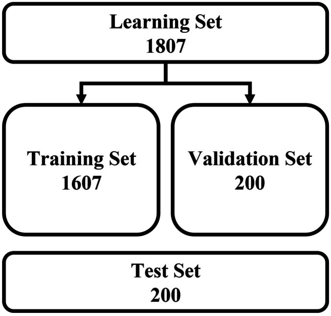
Overview of image data allocation for training the Mask R-CNN model

Sagittal Radiographic Parameters

Spino-pelvic parameters were selected with reference to the Scoliosis Research Society (SRS) Schwab ASD classification based on spino-pelvic parameters, which are widely used to evaluate and treat patients with spinal deformity, as proposed by Schwab et al. [2]. Thoracic kyphosis (TK), thoracic lumbar kyphosis (TLK), sacral slope (SS), LL, PT, PI, and SVA were included as measurement parameters.

SVA is defined as the length of a horizontal line connecting the posterior superior sacral endplate to a vertical plumbline dropped from the centroid of the C7 vertebral body (Fig. 3a). TK is the Cobb’s angle measured between the T4 upper endplate and the T12 lower endplate. TLK is between the T10 upper endplate and the L2 lower endplate, and LL is between the L1 upper endplate and the sacral endplate (Fig. 3b). SS denotes the slope of the sacral endplates, the angle between which is measured relative to the horizontal reference line. Furthermore, PT was measured as the angle between the vertical reference line and the line connecting the hip axis (HA) to the midpoint of the sacral endplate, where the sagittal coordinates of the HA were measured as the center of gravity of the two femoral heads. PI is the angle between the line connecting the HA to the midpoint of the sacral endplate and the orthogonal line passing through the midpoint of the sacral endplate, calculated as the sum of the SS and PT (Fig. 3c).

Fig. 3.

Methods for measuring spinal parameters. a SVA was measured from the C7 and sacral vertebrae. b TK, TLK, and LL were measured in T4-T12, T10-L2, and L1-sacrum, respectively. c SS is the slope of the straight line through the left and top points (red points) of the sacral endplate, and PT was estimated from the line through the HA at the midpoint (green points) of the sacral endplate. d An example of upper and lower endplate slope measurement

Development of an Automated Measurement Pipeline for Alignment Analysis in Whole-Spine Lateral Radiographs

Mask R-CNN [21], a popular algorithm for instance segmentation, is used to detect individual ROIs corresponding to each class (C7 vertebra, T4-L5 vertebrae, sacrum, and femoral heads) and create a mask. Mask R-CNN is adapted from the MMDetection tool, a set of tools for object detection developed by open-mmlab [22].

Mask R-CNN consists of two steps. The first stage consists of a region proposal network (RPN), which generates proposals of regions of interest. The second step predicts the object’s class and creates a bounding box and binary mask. Contrast-limited adaptive histogram equalization is applied to all input images for Mask R-CNN, and ResNeXt-101(32 × 4d)-FPN (Feature Pyramid Network) [23] is used as the backbone of the proposed Mask R-CNN. Then, using the generated feature maps, RPN finds all candidate regions. Next, high-quality instance segmentation masks of detected objects are generated via ROI classifier and bounding box regressor (Fig. 4).

Fig. 4.

Block diagram of Mask R-CNN algorithm for spine segmentation (FM = feature maps; RPN = region proposal network; FCN = fully connected network; FC layer = fully connected layer)

A computer vision pipeline has been developed to identify key landmarks on the vertebral bodies and femoral heads' binary masks generated by the instance segmentation model, and measure and visualize the spino-pelvic parameters. First, an algorithm for handling exceptions in incorrect parameter measurements was developed based on the open-source computer vision library (OpenCV). This algorithm checks the overlap degree, distance, and the number of vertebral bodies closest to the sacrum in the binary mask, using this information to detect segmentation errors and exclude them from the relevant measurements. In the binary masks meeting these conditions, the algorithm to identify key landmarks uses the OpenCV function findContours to locate the contours of the vertebral bodies and femoral heads. The contour coordinates are approximated to polygons with fewer vertices using the OpenCV function approxPolyDP [24] to obtain the end points of the vertebral endplates (${P1}_{\mathit{endplate}}$, ${P2}_{\mathit{endplate}}$). The obtained key points are then used to calculate the slope of the vertebral endplates for calculating TK, TLK, and LL.

Figure 5 shows the process of the DP algorithm. Point $P_1$ with the maximum vertical distance from the line connecting the start point $P_{\mathit{start}}$ and end point $P_{\mathit{end}}$ of the contour was acquired. $l_1$ is a straight line connecting the $P_{\mathit{start}}$ and$P_1$. Point $P_2$ with the maximum vertical distance from $l_1$ was found then verified if ${\mathit{Dist}}_{\mathit{max}}$ was less than $\epsilon$. If ${\mathit{Dist}}_{\mathit{max}}$ was less than$\epsilon$, then $P_{\mathit{start}}$ and $P_2$ were inserted into the point list of the polygon approximation. If ${\mathit{Dist}}_{\mathit{max}}$ was greater than or equal to$\epsilon$, a new baseline $l_2$ with points $P_{\mathit{start}}$ and $P_2$ was drawn, and ${\mathit{Dist}}_{\mathit{max}}$ was recalculated based on $l_2$ and then repeated. As a result, the vertebral body was approximated with four points, with coordinates corresponding to each vertex. For example, in Fig. 3d, the endpoints of the upper endplate were two red points, separated by the left point ${P1}_{\mathit{endplate}}$ ($x_1$,$y_1$) and the right point ${P2}_{\mathit{endplate}}$ ($x_2$,$y_2$). The slope of the sacral endplate was calculated from two points: the left point with the smallest x-coordinate and the top point with the smallest y-coordinate among the detected contour coordinates. The slope of the endplates can be obtained using Eq. (1):

$$m=\frac{y_2-y_1}{x_2-x_1}$$ 1

where m represents the slope of the straight line connecting the two points. The angle of intersection of $m_1$ and $m_2$ corresponding to the two endplate slopes is calculated using Eq. (2) as:

$$Angle={\tan }^{-1}\left|\frac{m_1-m_2}{1+m_1{m}_2}\right|$$ 2

Fig. 5.

Vertebral body polygon approximation procedure of DP algorithm. a When ${\mathit{Dist}}_{\mathit{max}}$ ≥ $\epsilon$ from $l_1$, $P_{\mathit{start}}$ and $P_2$ are then used for the baseline. b ${\mathit{Dist}}_{\mathit{max}}$ is computed at the points between $P_{\mathit{start}}$ and $P_2$. When ${\mathit{Dist}}_{\mathit{max}}$ < $\epsilon$ from $l_2$, $P_2$ becomes the starting point. c When ${\mathit{Dist}}_{\mathit{max}}$ ≥ $\epsilon$ from $l_2$, $P_2$ and $P_3$ are used for the next baseline. d ${\mathit{Dist}}_{\mathit{max}}$ is calculated at the points between $P_2$ and $P_3$. When ${\mathit{Dist}}_{\mathit{max}}$ < $\epsilon$ from $l_2$, $P_3$ becomes the starting point. e, f The repetition of the above process

The sagittal coordinates of the HA for the calculation of pelvic parameters are obtained from the centroid of the binary mask. The centroid coordinates of the C7 vertebra for calculating the SVA and the sagittal coordinates of the posterior superior sacral endplate are also obtained based on the position information of the detected contour coordinates by computer vision algorithms. Subsequently, the spinal parameters are automatically calculated and visualized (see Fig. 6). Finally, this computer vision pipeline was integrated with an instance segmentation model to build an automated parameter measurement pipeline without manual intervention.

Fig. 6.

Computer vision analysis results for predicted and ground truth masks. a Lateral X-ray images. b Ground truth images. c Predicted images of Mask R-CNN model. d Vertebral bodies in the T4-L5 vertebrae class are identified based on the central coordinates of the sacral. e The results of parameter measurement of the computer vision algorithm were visualized

Training Model and Evaluation Methods

X-ray images of various sizes in the dataset are automatically resized to a maximum of 1333 × 800 scale [25]. The Mask R-CNN model is trained for 36 epochs, and the optimizer is stochastic gradient descent (SGD) with momentum. A Linux workstation with two NVIDIA RTX 2080TI GPUs was used to train and test the Mask R-CNN model. Torchvision 0.13.1, openCv 4.6.0, mmcv 1.6.1, and MMDetection 2.25.2 are installed in the experimental environment. The details of the training parameters presented in Table 2.

Table 2.

Hyperparameter setting

Hyperparameter	Configuration
Optimizer	Stochastic gradient descent (SGD)
Learning rate	0.005
Learning rate decay	0.0001
Epoch	36
Momentum parameter	0.9
Batch size	2

In general, the multi-task loss (L) of the Mask R-CNN model is defined as the sum of classification (L_cls), localization (L_box), and segmentation mask (L_mask) losses. L_cls and L_mask are classical binary cross-entropy losses, while L_box is a smoothL1 loss [21]. The first evaluation metrics, including precision, recall, loss, and confidence scores, were measured using the MMDetection tool. Additionally, the Dice similarity coefficient (DSC) was calculated. DSC is a validated metric for segmentation that evaluates the quality of the segmentation model compared to reality. DSC can be calculated as the Area of overlap divided by the sum of the number of pixels in the predicted mask and the ground truth mask. The second evaluation metric includes average precision (AP) and average recall (AR). AP represents the area under the precision-recall curve for each class, while AR is defined as twice the area under the Recall-Intersection over Union (IoU) curve for each class. For the COCO format, both AP and AR calculations are averaged across all categories, considering IoU thresholds ranging from 0.5 to 0.95 at intervals of 0.05 [26, 27].

Statistical Analysis

Sagittal radiographic parameters were measured on a test set of radiographs. The measurements obtained from an automated measurement algorithm and two other surgeons (surgeon 1 and surgeon 2) were compared to the measurements of the criterion standard surgeon. Furthermore, the average of the three surgeons' manual measurements was also compared to the algorithm’s measurements. Performance was evaluated by comparing manual measurements with those from an automated measurement algorithm using computer-vision. Pearson’s correlation analysis was used to investigate the correlation between automated and manual measurements. The significance level was set at p < 0.05. Moreover, Bland–Altman plots were used to evaluate the similarity of measurements between the criterion standard and the automated measurement algorithm [28]. The intraclass correlation coefficient (ICC) values were used to evaluate the reliability between the criterion standard and automated measurement algorithm. ICC of 0.0–0.24, 0.25–0.49, 0.50–0.69, 0.70–0.89, and 0.90–1.0 were classified as absent to poor, low, fair/moderate, good, and excellent reliability, respectively [18, 29]. Statistical analyses were performed using Statistical Package for Social Sciences (Version 21.0; IBM, Armonk, NY, USA).

Results

Performance of Spine Segmentation

The manual measurements by a human observer were performed using 200 test images. As a result of the Mask R-CNN model, predictive image generation was performed from C7 to the femoral head. Mask R-CNN model achieved an AP⁵⁰ of 96.2% and DSC of 92.6% for the spine segmentation task in the test set (Table 3).

Table 3.

Parameters for evaluating the experimental results of the spine segmentation

Annotation type	AP	AP50	AP75	AR	DSC
Segmentation mask	64.90%	96.20%	75.70%	70.40%	92.60%
Detection box	71.60%	97%	83.60%	77.30%
Class-wise AP	C7		T4-L5 vertebrae	Sacrum	Femoral heads
Segmentation mask	47.50%		79.70%	63.70%	68.80%
Detection box	54.80%		81.50%	77.50%	73%

AP and AR are averaged over 10 intersection over union (IoU) thresholds, ranging from 0.5 to 0.95 at intervals of 0.05. AP⁵⁰ is computed at a single IoU of 0.5. AP⁷⁵ is computed at a single IoU of 0.75

The number of individually identified vertebral bodies in class T4-L5 vertebrae was 14, with nine vertebral bodies including T4-T12 and five vertebral bodies including L1-L5. However, if the number of individually identified vertebral bodies in class T4-L5 vertebrae because of sacralization or lumbarization was 13 or 15, we identified four or six lumbar vertebrae. In a total of 200 test set radiographs, six images had 13 class T4-L5 vertebrae instead of the expected 14. Despite these discrepancies, these images were also able to measure parameters normally in our computer vision-based automated measurement algorithm. However, these cases were excluded from statistical analysis for comparison with manual measurement methods. Six failure cases of the spine segmentation model were also excluded from statistical analysis. There was one case of unsuccessful segmentation in which T4 vertebral body segmentation failed and five cases in which the sacral and L5 masks overlapped (Fig. 7). The reason for the failure in T4 segmentation is a continuation of the thoracic vertebrae identification problem caused by radiopaque artifacts, and the overlapping issue between the sacrum and L5 is inferred to be a problem arising from the small number of sacralization cases in the training set.

Fig. 7.

There were two types of failed inference results from the Mask R-CNN model on the test-set. a T4 segmentation failure image. b Case of segmentation failure where the sacrum and L5 overlap

Descriptive Statistics

The sagittal radiographic parameters for the test dataset (200 images), as determined by the criterion standard surgeon, are presented in Table 4, including the mean and median values. The algorithms, surgeon 1, and surgeon 2 were compared to the criterion standard surgeon, and the absolute differences in measurements were expressed as mean and median values in Table 5. The largest mean and median values of difference were 3.0° and 2.5°, respectively. The values of mean absolute error (MAE) ranged from 0.4° to 3.0° for all parameters compared with the criterion standard. In general, the algorithm’s measurement results showed a strong correlation with manual measurements in all cases, with p < 0.001. The slope of the regression line was between 44° and 49°, which was relatively close to the ideal 45°. The standard error of estimate (SEE), defined as the standard deviation of the difference between an estimate using an automated measurement algorithm and the ground truth, was within the 0.5° to 4.0° range compared with manual angle measurement (Table 6). The SEE value of SVA showed 1.2 mm. PI exhibited the largest SEE (4.0°); however, the MAE between the measured and predicted values was 3.0°, similar results were observed for the LL (SEE = 3.9°, MAE = 3.0°) and SS (SEE = 3.9°, MAE = 2.9°). Furthermore, SEE (0.5°) and MAE (0.4°) demonstrated the lowest PT values.

Table 4.

Descriptive statistics of sagittal radiographic parameters as determined by the criterion standard surgeon

Parameters	Manual measurement (°)
	Mean (SD)	Min	Median (IQR)	Max
TK	29.0 (10.2)	0.2	29.7 (13.5)	54.1
TLK	9.7 (7.6)	0.1	7.9 (10.6)	37.1
LL	46.8 (10.7)	11.7	47.5 (12.8)	74.9
PI	51.8 (9.4)	26.0	51.4 (11.7)	84.6
PT	16.0 (7.7)	− 8.4	15.0 (10.6)	40.0
SS	35.8 (6.4)	15.5	36.0 (7.2)	57.6
SVA (mm)	13.3 (35.9)	− 100.5	10.0 (41.7)	129.7

TK thoracic kyphosis (T4-T12), TLK thoracic lumbar kyphosis (T10-L2), LL lumbar lordosis (L1-Sacrum), SS sacral slope, PT pelvic tilt, PI pelvic incidence, SVA sagittal vertical axis

Table 5.

Performance evaluation of the sagittal radiographic parameters of the algorithm

Parameters		Operator	Absolute difference		Correlation analysis		ICC (95% CI)
			Mean (SD)	Median (IQR)	R	p value
Relative to criterion standard (°)
TK	Algorithm		2.7 (1.7)	2.5 (2.3)	0.980		0.97 (0.72–0.99)
	Surgeon 1		4.6 (3.0)	4.5 (3.8)	0.879	< 0.001*	0.93 (0.91–0.95)
	Surgeon 2		5.1 (3.3)	4.9 (4.1)	0.850		0.92 (0.89–0.94)
TLK	Algorithm		1.5 (1.1)	1.2 (1.7)	0.971		0.98 (0.98–0.99)
	Surgeon 1		4.1 (3.2)	3.4 (4.8)	0.818	< 0.001*	0.89 (0.86–0.92)
	Surgeon 2		4.6 (3.5)	3.8 (5.5)	0.810		0.88 (0.84–0.91)
LL	Algorithm		3.0(2.8)	2.2(3.5)	0.930		0.95 (0.94–0.97)
	Surgeon 1		4.3 (3.9)	3.2 (4.9)	0.883	< 0.001*	0.93 (0.91–0.95)
	Surgeon 2		4.9 (4.4)	3.7 (5.8)	0.859		0.92 (0.89–0.94)
PI	Algorithm		3.0(2.9)	2.1(3.4)	0.904		0.95 (0.93–0.96)
	Surgeon 1		4.6 (3.9)	3.4 (5.1)	0.827	< 0.001*	0.90 (0.87–0.93)
	Surgeon 2		4.4 (4.4)	3.2 (4.8)	0.824		0.90 (0.86–0.92)
PT	Algorithm		0.4(0.4)	0.3(0.3)	0.998		0.99 (0.99–0.99)
	Surgeon 1		1.8 (1.8)	1.4 (1.6)	0.945	< 0.001*	0.97 (0.96–0.98)
	Surgeon 2		1.6 (1.6)	1.2 (1.4)	0.961		0.98 (0.97–0.98)
SS	Algorithm		2.9(2.7)	2.1(3.4)	0.797		0.86 (0.81–0.90)
	Surgeon 1		4.4 (4.2)	3.2 (5.3)	0.702	< 0.001*	0.80 (0.74–0.85)
	Surgeon 2		3.9 (3.6)	2.8 (4.5)	0.735		0.84 (0.78–0.88)
SVA (mm)	Algorithm		1.2(1.1)	1.0(1.1)	0.999		0.99 (0.99–0.99)
	Surgeon 1		4.1 (3.6)	3.4 (3.6)	0.989	< 0.001*	0.99 (0.99–0.99)
	Surgeon 2		3.9 (3.4)	3.2 (3.3)	0.990		0.99 (0.99–0.99)
Relative to surgeon average (°)
TK			3.1 (3.0)	2.2 (3.6)	0.943		0.95 (0.85–0.98)
TLK			2.2 (2.3)	1.4 (2.1)	0.918		0.95 (0.94–0.97)
LL			2.9 (3.9)	1.4 (4.3)	0.912		0.94 (0.92–0.95)
PI	Algorithm		2.8 (3.1)	1.7 (3.3)	0.899	< 0.001*	0.94 (0.93–0.96)
PT			0.7 (0.8)	0.4 (0.8)	0.991		0.99 (0.99–0.99)
SS			2.6 (3.1)	1.3 (4.1)	0.793		0.86 (0.82–0.90)
SVA	(mm)		1.7 (1.6)	1.3 (1.6)	0.998		0.99 (0.99–0.99)

The asterisk (*) indicates statistical significance between the groups

TK thoracic kyphosis (T4-T12), TLK thoracic lumbar kyphosis (T10-L2), LL lumbar lordosis (L1-Sacrum), SS sacral slope, PT pelvic tilt, PI pelvic incidence, SVA sagittal vertical axis, ICC intraclass correlation coefficient

Table 6.

Regression analysis

Parameters	Slope of the regression line	Standard error of the estimate	R2
TK	47°	2.0°	0.961
TLK	46°	1.8°	0.942
LL	49°	3.9°	0.864
PI	44°	4.0°	0.817
PT	45°	0.5°	0.996
SS	46°	3.9°	0.635
SVA	44°	1.2 mm	0.999

TK thoracic kyphosis (T4-T12), TLK thoracic lumbar kyphosis (T10-L2), LL lumbar lordosis (L1-Sacrum), SS sacral slope, PT pelvic tilt, PI pelvic incidence, SVA sagittal vertical axis

Performance Evaluation of the Sagittal Radiographic Parameters

Pearson correlation analysis, Bland–Altman plot, and ICC analysis were used to validate the performance of the automated analysis algorithms for TK, TLK, LL, SS, PT, PI, and SVA The Pearson correlation between manual measurement and the computer vision algorithm exhibited strong quantitative correlation coefficients for all parameters (p < 0.001) (Table 5).

As shown in the Bland–Altman plot (Fig. 8), the mean differences between the Criterion Standard Surgeon and automated measurement algorithm were negligible relative to the magnitude of all the parameters. The small mean difference between actual and predicted values did not demonstrate any consistent bias between the two methods. However, the 95% confidence interval showed large limits of agreement amplitudes of 16.1°, 15.8°, and 15.1° for LL, PI, and SS measurements, respectively. This variability diminishes the direct clinical usefulness of automated measurement algorithms. Additionally, TK, TLK, and SVA had limits of agreement amplitudes of 8.2°, 7.2°, and 6.3 mm, respectively, while PT had a value of 2.0°, which could be estimated more reliably. The Bland–Altman plot also implies that the measured and expected results were very similar because most values were within a narrow 95% confidence interval. ICCs between manual and algorithm measurements were achieved good and excellent reliability in all parameters (Table 5).

Fig. 8.

Bland–Altman plots: kyphosis and spino-pelvic parameters

Discussion

Radiographic examination is a crucial tool in diagnosing spinal disorders, and accurate measurement of spinal-pelvic parameters using radiographs is essential for characterizing clinical entities and planning treatment. In this study, we present a fully automated pipeline for measuring spinal parameters from whole-spine lateral radiographs. Our pipeline utilizes Mask R-CNN [21] for vertebrae segmentation, and achieves an average Dice Similarity Coefficient (DSC) of 92.6% on a test set of 1,607 images. Previously reported methods for spinal segmentation have shown a DSC range of 82.1–95.1%, which is similar to the prediction accuracy of our model [30–33]. Consequently, the automatically segmented ROIs in our study provided reliable spino-pelvic parameter measurements. Results of Bland–Altman analysis on our predicted segmentations showed low bias and agreement limits within 10% compared to the mean of the measured values, with the highest value of 8.3% for TK and the remaining measurements ranging from 0.6 to 2.8% (Fig. 8). Our results showed ICC with values greater than 0.900 for all parameters but SS, indicating excellent inter-observer reliability between the automated measurement algorithm and human observer. While the inter-observer reliability value of SS indicated sufficient performance when measuring SS, the ICC of SS being the lowest out of all parameters indicated relatively high variability in the current sacral segmentation performance or sacral slope estimation of the computer vision algorithm. Issues in determining SS parameters can be attributed to common segmentation failures that occurred at the sacral endplate. While failure cases were excluded from the statistics, ICC results suggest that the segmentation performance of the sacral endplate requires improvement. Additional reinforcement of training datasets with additional clinical cases can reduce these problems. Alternatively, new considerations in computer vision techniques for estimating sacrum endplates may be required.

Manual measurements obtained by our three surgeons show a trend consistent with previous studies. A previous study found that in manual measurements of spino-pelvic parameters in 49 adult whole-spine digital radiographs, including SS, PT, PI, and TK, the ICC score ranged from 0.82 to 0.99, and the standard error of measurement was between 0.8° and 4.9°. For SVA, the range was between 2.2 and 5.8 mm [34]. In another study examining SS, PT, PI, LL, and TK in 50 ASD patients, the ICC score ranged from 0.91 to 0.98, the MAE ranged from 0.12° to 5.25°, and for SVA, it was 2.04 mm [35]. In our study, the ICC scores ranged from 0.80 to 0.99, the MAE ranged from 1.6° to 5.1°, and the range for SVA was between 3.9 and 4.1 mm.

The results of our automated spinal parameter measurement pipeline demonstrated a performance comparable to that of the criterion standard surgeon. The MAE and SEE values for the parameters, obtained using our automated method, ranged from 0.4° to 3.0° and 0.5° to 4.0°, respectively, while the SVA value was 1.2 mm. Furthermore, due to its non-stochastic nature, the computer vision-based measurement algorithm exhibited perfect reproducibility, with an intraclass correlation coefficient of one. The algorithm showed a smaller MAE than surgeon 1 and surgeon 2 for all measurements compared to the criterion standard. Moreover, when compared to the overall surgeon average, the algorithm also exhibited smaller mean and median absolute differences for all measurements, suggesting that it generalizes well to surgeon measurements.

Recently, there has been a growing interest in fully automated software tools. A previous study applied to measuring spinal parameters, Galbusera et al. was able to apply a fully connected network to extract 78 landmarks from biplanar X-ray images acquired using an EOS imaging system, including images from various age groups and spinal deformities. For TK, LL, SS, PT, and PI, the ME and SEE ranged from 2.7° to 11.5° and 0.7° to 7.6°, respectively [17]. Cho et al. used a U-Net segmentation model to identify the L1 and sacrum. Their automated measurement algorithm achieved mean and median absolute errors of 8.055° and 6.965°, respectively [30]. Korez et al. utilized two machine learning algorithms, RetinaNet and U-Net, to determine SS, PT, and PI, achieving MAE values in the range of 2.7° to 5.5° [20]. Schwartz et al. trained the MultiResUNet segmentation model. Images with spinal instruments and hip arthroplasty were included in the data set. For LL, SS, PT, and PI, MAE values range from 2.1° to 4.8° [31]. Yeh et al. predicted 45 landmark coordinates from whole-spine lateral radiographs and automatically measured 18 spino-pelvic parameters. For T5-T12 main thoracic kyphosis, LL, PT, and PI, the MAE values range from 1.1° to 5.1°. For the SVA, the MAE value is 1.9 mm [19]. Compared to previous studies of automatic parameter measurement, our results show similar or better performance. In particular, our automated measurement pipeline is applicable to general X-ray images, and it is suitable for universal use.

Even in extreme cases of images with spinal instruments, bone cements, and fractures, our model was able to produce partially successful results, which can be further built upon for a more accurate parameter evaluation (Fig. 9) [36]. Finally, very few studies have comprehensively measured fundamental spino-pelvic parameters using whole-spine radiographs, often excluding parameters such as SVA, an important and reliable radiological predictor for assessing sagittal balance. Providing surgeons with reproducible visualizations of these important predictors and spine segmentation results can be clinically useful for diagnosis and treatment planning such as vertebral body identification.

Fig. 9.

Vertebral segmentation results of Mask R-CNN in an untrained clinical case. a Spinal instruments. b Fractured vertebrae. c Bone cement

The limitations of this study are as follows. Images with severe spinal deformities and implants were excluded from the training data, and T1 to T3 vertebral bodies were not labeled because of visual inspection and training data construction difficulties. While this simplifies the labeling task and computer vision algorithms for better results, it reduces the clinical usefulness of our tool in postoperative follow-up studies. Particularly, the automatic segmentation of T1–T3 may require a completely novel method because of anatomical obstruction present in X-rays preventing even manual delineation of T1-T3. Follow-up studies monitoring patients' spinal parameters over time or before and after surgical or non-surgical treatments are essential for the automatic parameter measurement algorithm to perform effectively in clinical workflows. Hence, it is essential to obtain a training dataset of images that includes all vertebral malformations and implants.

Conclusions

We propose a computer vision pipeline that automatically measures spino-pelvic parameters, including SVA, from whole-spine lateral radiographs. The proposed fully automated pipeline was able to measure spinal parameters reproducibly and with reduced inter-rater variability. In addition, the results of spine segmentation can play an auxiliary role in visually helping surgeons to interpret images more quickly and accurately. Therefore, the spine segmentation-based automated measurement and analysis pipeline with the computer vision algorithm presented in this study can be integrated into clinical and digitally assisted diagnostic pipelines.

Author Contribution

Yong-Tae Kim: conceptualization, methodology, formal analysis, data curation, investigation, software, validation, visualization, writing—original draft, writing—review and editing. Tae Seok Jeong: conceptualization, methodology, formal analysis, data curation, investigation, writing—original draft, writing—review and editing. Young Jae Kim: conceptualization, methodology, project administration, formal analysis, data curation, supervision, writing—review and editing. Woo Seok Kim: conceptualization, methodology, project administration, formal analysis, data curation, supervision, writing—review and editing. Kwang Gi Kim: conceptualization, methodology, supervision, funding acquisition, project administration, writing—review and editing. Gi Taek Yee: conceptualization, methodology, supervision, funding acquisition, project administration, writing—review and editing.

Funding

This work was supported by the Gachon University (GCU-202205980001).

Availability of Data and Material

Not applicable.

Code Availability

Not applicable.

Declarations

Ethics Approval

The study was conducted according to the guidelines of the Declaration of Helsinki and approved by the Institutional Review Board of Gil Medical Center (GDIRB-2022-190).

Consent to Participate

Informed consent was obtained from all individual participants included in the study.

Consent for Publication

Patients signed informed consent regarding publishing their data.

Conflict of Interest

The authors declare no competing interests.

References

- 1.Schwab F, Dubey A, Gamez L, El Fegoun AB, Hwang K, Pagala M, Farcy JP. Adult scoliosis: prevalence, SF-36, and nutritional parameters in an elderly volunteer population. Spine. 2005;30(9):1082–1085. doi: 10.1097/01.brs.0000160842.43482.cd. [DOI] [PubMed] [Google Scholar]
- 2.Schwab F, Ungar B, Blondel B, Buchowski J, Coe J, Deinlein D, DeWald C, Mehdian H, Shaffrey C, Tribus C, Lafage V. Scoliosis Research Society—Schwab adult spinal deformity classification: a validation study. Spine. 2012;37(12):1077–1082. doi: 10.1097/BRS.0b013e31823e15e2. [DOI] [PubMed] [Google Scholar]
- 3.Schwab FJ, Blondel B, Bess S, Hostin R, Shaffrey CI, Smith JS, Boachie-Adjei O, Burton DC, Akbarnia BA, Mundis GM, Ames CP. Radiographical spinopelvic parameters and disability in the setting of adult spinal deformity: a prospective multicenter analysis. Spine. 2013;38(13):E803–E812. doi: 10.1097/BRS.0b013e318292b7b9. [DOI] [PubMed] [Google Scholar]
- 4.Smith JS, Bess S, Shaffrey CI, Burton DC, Hart RA, Hostin R, Klineberg E, International Spine Study Group. Dynamic changes of the pelvis and spine are key to predicting postoperative sagittal alignment after pedicle subtraction osteotomy: a critical analysis of preoperative planning techniques. Spine. 2012 May 1;37(10):845–53. 10.1097/BRS.0b013e31823b0892 [DOI] [PubMed]
- 5.Glassman SD, Bridwell K, Dimar JR, Horton W, Berven S, Schwab F. The impact of positive sagittal balance in adult spinal deformity. Spine. 2005;30(18):2024–2029. doi: 10.1097/01.brs.0000179086.30449.96. [DOI] [PubMed] [Google Scholar]
- 6.Lamartina C, Berjano P, Petruzzi M, Sinigaglia A, Casero G, Cecchinato R, Damilano M, Bassani R. Criteria to restore the sagittal balance in deformity and degenerative spondylolisthesis. European spine journal. 2012;21(1):27–31. doi: 10.1007/s00586-012-2236-9. [DOI] [PMC free article] [PubMed] [Google Scholar]
- 7.Lafage V, Schwab F, Patel A, Hawkinson N, Farcy JP. Pelvic tilt and truncal inclination: two key radiographic parameters in the setting of adults with spinal deformity. Spine. 2009;34(17):E599–606. doi: 10.1097/BRS.0b013e3181aad219. [DOI] [PubMed] [Google Scholar]
- 8.Schwab F, Patel A, Ungar B, Farcy JP, Lafage V. Adult spinal deformity—postoperative standing imbalance: how much can you tolerate? An overview of key parameters in assessing alignment and planning corrective surgery. Spine. 2010;35(25):2224–2231. doi: 10.1097/BRS.0b013e3181ee6bd4. [DOI] [PubMed] [Google Scholar]
- 9.Carman DL, Browne RH, Birch JG. Measurement of scoliosis and kyphosis radiographs. Intraobserver and interobserver variation. JBJS. 1990;72(3):328–333. [PubMed] [Google Scholar]
- 10.Chen YL. Vertebral centroid measurement of lumbar lordosis compared with the Cobb technique. Spine. 1999;24(17):1786. doi: 10.1097/00007632-199909010-00007. [DOI] [PubMed] [Google Scholar]
- 11.Harrison DE, Harrison DD, Cailliet R, Troyanovich SJ, Janik TJ, Holland B. Cobb method or Harrison posterior tangent method: which to choose for lateral cervical radiographic analysis. Spine. 2000;25(16):2072–2078. doi: 10.1097/00007632-200008150-00011. [DOI] [PubMed] [Google Scholar]
- 12.Harrison DE, Cailliet R, Harrison DD, Janik TJ, Holland B. Reliability of centroid, Cobb, and Harrison posterior tangent methods: which to choose for analysis of thoracic kyphosis. Spine. 2001;26(11):e227–e234. doi: 10.1097/00007632-200106010-00002. [DOI] [PubMed] [Google Scholar]
- 13.Krupinski EA. Current perspectives in medical image perception. Attention, Perception, & Psychophysics. 2010;72(5):1205–1217. doi: 10.3758/APP.72.5.1205. [DOI] [PMC free article] [PubMed] [Google Scholar]
- 14.Shea KG, Stevens PM, Nelson M, Smith JT, Masters KS, Yandow S. A comparison of manual versus computer-assisted radiographic measurement: intraobserver measurement variability for Cobb angles. Spine. 1998;23(5):551–555. doi: 10.1097/00007632-199803010-00007. [DOI] [PubMed] [Google Scholar]
- 15.Vrtovec T, Pernuš F, Likar B. A review of methods for quantitative evaluation of spinal curvature. European spine journal. 2009;18:593–607. doi: 10.1007/s00586-009-0913-0. [DOI] [PMC free article] [PubMed] [Google Scholar]
- 16.Gstoettner M, Sekyra K, Walochnik N, Winter P, Wachter R, Bach CM. Inter-and intraobserver reliability assessment of the Cobb angle: manual versus digital measurement tools. European Spine Journal. 2007;16:1587–1592. doi: 10.1007/s00586-007-0401-3. [DOI] [PMC free article] [PubMed] [Google Scholar]
- 17.Galbusera F, Niemeyer F, Wilke HJ, Bassani T, Casaroli G, Anania C, Costa F, Brayda-Bruno M, Sconfienza LM. Fully automated radiological analysis of spinal disorders and deformities: a deep learning approach. European Spine Journal. 2019;28(5):951–960. doi: 10.1007/s00586-019-05944-z. [DOI] [PubMed] [Google Scholar]
- 18.Illés T, Somoskeöy S. The EOS™ imaging system and its uses in daily orthopaedic practice. International orthopaedics. 2012;36(7):1325–1331. doi: 10.1007/s00264-012-1512-y. [DOI] [PMC free article] [PubMed] [Google Scholar]
- 19.Yeh YC, Weng CH, Huang YJ, Fu CJ, Tsai TT, Yeh CY. Deep learning approach for automatic landmark detection and alignment analysis in whole-spine lateral radiographs. Scientific reports. 2021;11(1):1–5. doi: 10.1038/s41598-021-87141-x. [DOI] [PMC free article] [PubMed] [Google Scholar]
- 20.Korez R, Putzier M, Vrtovec T. A deep learning tool for fully automated measurements of sagittal spinopelvic balance from X-ray images: performance evaluation. European Spine Journal. 2020;29(9):2295–2305. doi: 10.1007/s00586-020-06406-7. [DOI] [PubMed] [Google Scholar]
- 21.He K, Gkioxari G, Dollár P, Girshick R. Mask r-cnn. InProceedings of the IEEE international conference on computer vision 2017 (pp. 2961–2969). 10.1109/ICCV.2017.322
- 22.Chen K, Wang J, Pang J, Cao Y, Xiong Y, Li X, Sun S, Feng W, Liu Z, Xu J, Zhang Z. MMDetection: Open mmlab detection toolbox and benchmark. arXiv preprint arXiv:1906.07155. 2019 Jun 17. 10.48550/arXiv.1906.07155
- 23.Xie S, Girshick R, Dollár P, Tu Z, He K. Aggregated residual transformations for deep neural networks. InProceedings of the IEEE conference on computer vision and pattern recognition 2017 (pp. 1492–1500).
- 24.Ramer U. An iterative procedure for the polygonal approximation of plane curves. Computer graphics and image processing. 1972;1(3):244–256. doi: 10.1016/S0146-664X(72)80017-0. [DOI] [Google Scholar]
- 25.Kozlov A. Working with scale: 2nd place solution to Product Detection in Densely Packed Scenes [Technical Report]. arXiv preprint arXiv:2006.07825. 2020 Jun 14. 10.48550/arXiv.2006.07825
- 26.Hui J. mAP (mean Average Precision) for object detection. Jonathan Hui. 2018 Mar 7. [online] Available: https://medium.com/jonathan_hui/map-mean-average-precision-for-object-detection-45c121a31173.
- 27.Lin TY, Maire M, Belongie S, Hays J, Perona P, Ramanan D, Dollár P, Zitnick CL, Microsoft coco: Common objects in context. InEuropean conference on computer vision, 6. Cham: Springer; 2014. pp. 740–755. [Google Scholar]
- 28.Altman DG, Bland JM. Measurement in medicine: the analysis of method comparison studies. Journal of the Royal Statistical Society: Series D (The Statistician). 1983;32(3):307–317. doi: 10.2307/2987937. [DOI] [Google Scholar]
- 29.Kuklo TR, Potter BK, O'Brien MF, Schroeder TM, Lenke LG, Polly Jr DW, Spinal Deformity Study Group. Reliability analysis for digital adolescent idiopathic scoliosis measurements. Clinical Spine Surgery. 2005 Apr 1;18(2):152–9. 10.1097/01.brs.0000153702.99342.9c [DOI] [PubMed]
- 30.Cho BH, Kaji D, Cheung ZB, Ye IB, Tang R, Ahn A, Carrillo O, Schwartz JT, Valliani AA, Oermann EK, Arvind V. Automated measurement of lumbar lordosis on radiographs using machine learning and computer vision. Global Spine Journal. 2020;10(5):611–618. doi: 10.1177/2192568219868190. [DOI] [PMC free article] [PubMed] [Google Scholar]
- 31.Schwartz JT, Cho BH, Tang P, Schefflein J, Arvind V, Kim JS, Doshi AH, Cho SK. Deep learning automates measurement of spinopelvic parameters on lateral lumbar radiographs. Spine. 2021;46(12):E671–E678. doi: 10.1097/BRS.0000000000003830. [DOI] [PubMed] [Google Scholar]
- 32.Kim DH, Jeong JG, Kim YJ, Kim KG, Jeon JY. Automated vertebral segmentation and measurement of vertebral compression ratio based on deep learning in X-ray images. Journal of Digital Imaging. 2021;34:853–861. doi: 10.1007/s10278-021-00471-0. [DOI] [PMC free article] [PubMed] [Google Scholar]
- 33.Zhang L, Shi L, Cheng JC, Chu WC, Yu SC. LPAQR-Net: efficient vertebra segmentation from biplanar whole-spine radiographs. IEEE Journal of Biomedical and Health Informatics. 2021;25(7):2710–2721. doi: 10.1109/JBHI.2021.3057647. [DOI] [PubMed] [Google Scholar]
- 34.Kyrölä KK, Salme J, Tuija J, Tero I, Eero K, Arja H. Intra-and interrater reliability of sagittal spinopelvic parameters on full-spine radiographs in adults with symptomatic spinal disorders. Neurospine. 2018 Jun;15(2):175. 10.14245/ns.1836054.027 [DOI] [PMC free article] [PubMed]
- 35.Lafage R, Ferrero E, Henry JK, Challier V, Diebo B, Liabaud B, Lafage V, Schwab F. Validation of a new computer-assisted tool to measure spino-pelvic parameters. The Spine Journal. 2015;15(12):2493–2502. doi: 10.1016/j.spinee.2015.08.067. [DOI] [PubMed] [Google Scholar]
- 36.Konya S, Natarajan TS, Allouch H, Nahleh KA, Dogheim OY, Boehm H. Convolutional neural network-based automated segmentation and labeling of the lumbar spine X-ray. Journal of Craniovertebral Junction & Spine. 2021;12(2):136. doi: 10.4103/jcvjs.jcvjs_186_20. [DOI] [PMC free article] [PubMed] [Google Scholar]
Associated Data
This section collects any data citations, data availability statements, or supplementary materials included in this article.
Data Availability Statement