Principal Component Analysis of 1D ¹H Diffusion Edited NMR Spectra of Protein Therapeutics

Abstract

The one-dimensional (1D) diffusion edited proton NMR method, Protein Fingerprint by Lineshape Enhancement (PROFILE) has been demonstrated to be suitable for higher order structure (HOS) characterization of protein therapeutics including monoclonal antibodies. Recent reports in the literature have demonstrated its advantages for HOS characterization over traditional methods such as circular dichroism and Fourier-transform infrared spectroscopy. Previously, we have demonstrated that the PROFILE method is complementary with high resolution 2D methyl correlated NMR methods and how both may be deployed as a multi-modal platform to further the utility of NMR for HOS characterization. A major limitation of the PROFILE method remains its need for high signal to noise data due to its reliance on convolution difference processing and linear correlation metrics to assess spectral similarity. Here we present an alternative method for analyzing 1D diffusion edited spectra, which overcomes this limitation by using nonlinear iterative partial least squares (NIPALS) principal component analysis, and which we dub PROtein Fingerprint Observed Using NIPALS Decomposition (PROFOUND). We demonstrate that results from the PROFOUND method are robust with respect to instrument, operator and in the presence of high experimental noise and how it may be employed to provide quantitative assessment of spectral similarity.

Introduction

One-dimensional (1D) ¹H NMR methods are, in principle, well suited for the characterization of higher order structure (HOS) of protein therapeutics, including monoclonal antibodies (mAbs).^1–8 In contrast to current standard analytical technologies used to assess HOS of biotherapeutics, namely circular dichroism (CD) and Fourier transform infrared spectroscopy (FTIR), 1D ¹H NMR has the ability to report on all chemical environments of the protein analyte and is sensitive to all elements of HOS (i.e. 2°-4°) as well as sequence and post-translational modifications. Indeed, one recent study⁹ has demonstrated that the 1D ¹H NMR method, Protein Fingerprint by Lineshape Enhancement (PROFILE),² is fit-for-purpose at detecting higher order structural variation in biotherapeutic products as benchmarked against common biophysical techniques such as CD and FTIR.

We have recently reported on an inter-laboratory study¹⁰ comparing the performance of the 1D PROFILE method with the 2D ¹H-¹³C methyl HSQC method¹¹ for HOS characterization of mAbs. In that study, spectral similarity was assessed by linear correlation analysis using the maximum value of the normalized cross-correlation coefficient between two test spectra, as originally described for the PROFILE method. While it was useful to benchmark the two methods using this metric, it has been well documented that linear correlation analysis is poorly suited to assess similarity of 2D spectra of biotherapeutics, given the poor tolerance of linear-correlation to experimental noise.^12,13 Indeed, for the PROFILE method, based on results from the inter-laboratory study, it is recommended to collect initial spectra at signal to noise of greater than 2000:1, which at 600 MHz and employing an inverse cryogenically cooled probe can require ca. 512-1024 scans and an hour or more of measurement time for one experiment for typical mAb samples at 37 °C. For 2D methyl spectra, it has been demonstrated that assessment of spectral similarity by Principal Component Analysis (PCA) overcomes limitations of linear correlation analysis, being simultaneously extremely tolerant to high experimental noise and more sensitive to spectral variation.

PCA has previously been applied to 1D spectra of mAb therapeutics. In an elegant study, Chen and colleagues¹ analyzed 1D ¹H NOESY spectra of rituximab and infliximab via PCA to examine intra and inter-lot variability as well as biosimilar-originator comparison and identified spectral signatures of aggregation. While that study demonstrated the feasibility of such methods, due to the use of a 1D NOESY experiment, which yields good signal to noise (S/N), superior water suppression and baseline performance,¹⁴ it required deformulation and blanking of spectral regions with residual excipient signals. When characterization under formulated conditions is a paramount concern, the 1D ¹H diffusion edited Pulsed Field-Gradient Stimulated Echo (PFG-STE) based experiments such as employed in the PROFILE method is preferred given its ability to filter out most common excipient signals.^2,3 Given the considerable difference in performance and properties between the two experiments, additional study of PCA applied to 1D ¹H PFG-STE spectra biotherapeutics is warranted. To that end, using representative data from the previous interlaboratory study, as well as a panel of new mAb samples, we investigate the use of NIPALS¹⁵ based PCA applied directly to 1D diffusion edited ¹H NMR spectra for HOS assessment of biotherapeutics, specifically evaluating performance and robustness as a function of experimental S/N. We further demonstrate the quantitative use of PCA Z-score distances and confidence surface overlap as a measure of spectral similarity.¹⁶ It is expected that this new approach will outperform PROFILE to deliver a quantitative and reproducible metrics of spectral, and thus structural similarity, even when high S/N cannot be achieved. Given the integral nature of convolution difference (i.e. Lineshape Enhancement) and linear correlation analysis to spectral analysis by PROFILE, we dub this alternative PCA-based method PROtein Fingerprint Observed Using NIPALS Decomposition (PROFOUND).

Experimental

Sample Preparation

Samples were prepared as previously described.¹⁰ Briefly, the sample set consisted of NISTmAb PS-8670 (mAb-1) and a second IgG1k (mAb-2) with 86.4% sequence identity to NISTmAb, papain digest fragments of each mAb (Digest-1 and Digest-2) and Endo-S treated isoforms of both mAbs (EndoGly-1 and EndoGly-2). All samples were prepared at 40 mg/mL in 10 mmol/L sodium acetate-d₃, pH 5.2 with 3% D₂O. Additional sets of NISTmAb PS-8670 where prepared at 40 mg/mL in 25 mmol/L L-histidine, pH 6.0, 3% D₂O (mAb-1*). Unless otherwise noted, 180 μL of each samples were placed in 4 mm D₂O susceptibility matched symmetric microtubes (Wilmad, Vineland NJ), or 20 μL of each sample in capillary NMR tubes for microprobe data.

NMR Data Acquisition

Data were collected on a 600 MHz Bruker Avance I spectrometer equipped with a TXI room temperature inverse HCN probe or TXI room temperature 1.0 mm inverse HCN microprobe both with z-axis gradient systems, a 600 MHz Bruker Avance III spectrometer equipped with a TCI cryogenically cooled inverse HCN probe and z-axis gradient system and a 400 MHz Bruker Avance III with an inverse BBI HX probe and z-axis gradient system. All 1D ¹H PFG-STE spectra were acquired as previously described.¹⁰ Briefly, data were acquired with 31248 points (2.0 and 1.3 ms ¹H acquisition at 400 MHz and 600 MHz respectively) over a spectral width of 20 ppm centered on the water line, with a recycle delay of 2.5 s and a diffusion delay of 100 ms and a bipolar gradient strength of 65 G/cm. 1024 transients were collected unless otherwise described in the text. All data were acquired at 37 °C unless otherwise noted. Selected spectra are shown in Figure S1.

Data Processing and Statistical Analysis

All spectral processing in the present work was automated via C-shell and TCL scripts using the facilities of NMRPipe software (version 10.8 or higher) and its custom TCL interpreter nmrWish, so that the procedure presented here is fully customizable.^17–19 Workflow details are illustrated in Figure S2, and example commands are given in Figure S3. NMRPipe software, scripts, and data are available for download²⁰, and the software is also available on the NMRbox cloud computing platform.²¹ The only input required is a metadata table of spectra to process (Figure S4), and using this input, the steps of Fourier processing, phase and baseline correction, spectral alignment, and scaling were all performed automatically. Processing starts with conversion of vendor-format time-domain NMR data to a common format, so that all subsequent steps are vendor-neutral. Automated format conversion is available for Agilent/Varian, Bruker, and JEOL time-domain NMR data, and other formats can be accommodated.

Spectra were processed with a polynomial baseline correction and a 2 Hz exponential line broadening function. The water signal was removed by convolution with a masking step-function set to zero between 4 ppm and 5 ppm and exponentially ramped up to one from 3 ppm to 4 ppm and 5 ppm to 6 ppm. Data were aligned by iterative minimization of spectral root mean squared difference as outlined in Figure S2. Each spectrum was scaled to match the intensity of the reference-class (Figure S4) average spectrum using least-squares minimization, and the full digital resolution of the processed spectrum was retained, without binning or mean centering prior to PCA. The effect of the scaling and alignment procedures on subsequent PCA result is illustrated in Figure S5. For a collection of 25 spectra from five classes, the whole procedure took less than two minutes on a laptop computer, and PCA was accomplished in seconds. An example script and further details for the procedure is shown in Supplemental Information. It should be emphasized that the success of this automated procedure depends critically on good measurement technique that yields spectra without baseline roll, since such systematic distortions hinder automated phase correction and directly interfere with PCA.¹⁶

PCA was performed using the NIPALS algorithm¹⁵ in NMRPipe. NIPALS extracts components one at a time by finding a single component spectrum that best matches the series in a least-squares sense. This component spectrum is a linear combination of all the spectra in the series, and the coefficients for combining the spectra are the PCA score values for that component. Once a component has been calculated in this way, the component spectrum is scaled and subtracted from each spectrum in the series, and additional components can be calculated by repeating the procedure on the residual series from the previous component. Since the PCA scores are linear coefficients in a least-squares solution, adding random noise to the starting data does not change the underlying ideal value of the scores, it will only change the uncertainties in deriving them.

Quantitative analysis of PCA results was accomplished using variance-normalized Principal Component (PC) scores,

$$PC{N}_{i,j}=\frac{x_{i,j}-u_i}{{\sigma }_{total,i}}$$ eq. 1

where ${\text{x}}_{\text{i},\text{j}}$ is the a given PC score of the i^th PC in the j^th class, ${\text{u}}_{\text{i}}$ is the mean value over all classes in the i^th PC and ${\sigma }_{\mathrm{total},\text{I}}$ is the total standard deviation over all classes in the i^th PC, as well as PC Z-scores,¹⁶

$$X_{i,j}=\frac{x_{i,j}-u_{i,j}}{\sqrt{\frac{{\sigma }_{i,j}+\cdots {\sigma }_{i,n}}{n-1}}}$$ eq. 2

where ${\text{X}}_{\text{i},\text{j}}$ is a given Z score of the i^th principal component in the j^th class, ${\text{u}}_{\text{i},\text{j}}$ is the average value of the j^th class in the i^th principal component and ${\sigma }_{\text{i},\text{j}}$ is the standard deviation of the j^th class in the i^th PC and n is the total number of classes. The interclass separation was computed as the Euclidean distance of the 1^st and 2^nd or 2^nd and 3^rd Principal Component Z –scores as described in the text,

$$D_{i,j}=\sqrt{{\sum }_{P{C}_N=1}^n\left(X_{P{C}_N,i}-X_{P{C}_N,j}\right)}$$ eq. 3

Where ${\text{D}}_{\text{i},\text{j}}$ is the distance between the i^th and j^th classes. Associated errors were propagated from standard deviations about the class average values according to

$${\delta }_{i,j}=\frac{1}{D_{i,j}}\sqrt{\left[\left(X_{2,i}-X_{2,j}\right)*\left({\sigma }_{2,i}{}^2+{\sigma }_{2,j}{}^2\right)\right]+\left[\left(X_{3,i}-X_{3,j}\right)*({\sigma }_{3,i}{}^2+{\sigma }_{3,j}{}^2\right]}$$ eq. 4

The degree of agreement of comparisons between distances from various datasets was assessed via a Quality-factor²²

$$Q=\frac{\sqrt{\sum (\frac{{D_i-D_k)}^2}{N})}}{0.5\ast \left[\sqrt{\frac{\sum D_i{}^2}{N}}+\frac{\sum D_k{}^2}{N}\right]}$$ eq. 5

Where ${\text{D}}_{\text{k}}$ and ${\text{D}}_{\text{l}}$ are corresponding distances from datasets k and l and N is the total number of distances being compared.

PCA scoring plots were visualized using MATLAB (R2019A) as previously described.²³ S/N was calculated in Topspin (v.3.6.2) using the sino function over the signal region of 12 ppm to −2 ppm and noise region of −2.2 ppm to −4.5 ppm following initial processing with a Gaussian multiplication window function with a Lorentzian broadening factor of −1 and a Gaussian broadening factor of 0.005 with digital water filtering by time-domain Gaussian convolution difference with 0.1 ppm filter width applied to data prior to Fourier transform followed by manual phasing.

Results and Discussion.

The PROFILE method is based upon convolution difference.²⁴ Data are decomposed by multiplying the initially collected 1D ¹H diffusion edited spectrum (Figure 1A) with a Gaussian broadening function to produce a low resolution ‘contour’ component spectrum (Figure 1B). The contour component spectrum is then subtracted from the original spectrum to produce a highly resolved ‘fingerprint’ component spectrum (Figure 1C). Similarity between a pair of spectra is then assessed as the product of the cross-correlation coefficients between the two contour and two fingerprint component spectra.² While this increases the sensitivity to spectral variation of the method relative to direct comparison of the original data, it results in significantly lower S/N in the fingerprint sub-spectrum. Given the high S/N requirements to derive meaningful comparison from linear correlation analysis, this puts a substantial burden on collecting the initial data with adequate sensitivity. Coupled with the need to collect enough replicated measurements to statistically define the inherent measurement variability, for standard mAb samples, this can result in measurement times of approximately 6 hours per sample or about only three times faster than is required to collected the same number of 2D ¹H-¹³C methyl HSQC experiments. Such requirements severely limit the applicability of the method and fails to deliver on one of the main advantages of 1D ¹H approaches over a higher resolution 2D approach; significantly increased sensitivity/reduced experimental duration.

Figure 1.

Illustration of spectral decomposition by PROFILE using convolution difference (A-C) and by PROFOUND using NIPALS-PCA (D and E). The PROFILE method works by convolution difference of a 1D ¹H diffusion edited PFG-STE spectrum (A) by first generating a broadened contour spectrum by convolution with a Gaussian broadening function (B). The contour spectrum is then subtracted from the original spectrum to produce the fingerprint spectrum (C). The PRODOUND method employs PCA applied directly to a spectral intensity matrix from a series of spectra to produce a series average spectrum as a loading of the 1^st principal component (D). This average spectrum is then subtracted from all spectra in the series to produce 2^nd PC spectra; the second PC loading spectrum is the average of these spectra (E).

As an alternative, 1D diffusion edited spectra can be analyzed by PCA. While it might be considered that PCA could be applied to the sub-spectra following the convolution difference step, it can be rationalized that this only introduces additionally complexity and variability and that the initially collected PFG-STE data are the best input. If we consider the process of PCA, it can be justified why this is the case. If data are input directly following Fourier Transform and appropriate normalization (see Experimental: Data Processing and Statistical Analysis section), and not mean-centered beforehand, the first Principal Component (PC) represents the distribution of spectra about the average of the input series, and the first PC loading is the least-squares average spectrum of the input spectral series (Figure 1D). Conceptually, this is analogous to creating a Gaussian broadened contour spectrum to model the highly similar aspect of the spectra, except that with PCA the data alone determine the shape of the average spectrum and there is no dependence on an arbitrary broadening function. To determine the second PC, the first PC loading spectrum (Figure 1D) is subtracted from each of the original spectra (Figure 1A) in the series. This produces second PC sub-spectra that are highly reminiscent of the PROFILE ‘fingerprint’ sub-spectra (Figure 1E). Going forward, the series average second PC spectrum is then subtracted from all second PC sub-spectra to produce the third PC sub-spectra and so on until only noise is left. Thus, it can be seen that PCA and PROFILE at heart, decompose the data in a conceptually similar manner, only PCA incorporates additional dimensions of variability making it more sensitive to spectral variation and less susceptible to noise.

Preparation of Spectra for Comparison Using the Direct Spectra Matrix

PROFILE computes similarity from Fourier cross-correlation, which is not affected by spectral alignment. PCA, however correlates spectra directly, point by point, in the frequency domain, so scaling and alignment must be performed carefully. Critically, measurement and processing techniques need to be optimized to yield spectra without baseline distortion or phase distortion. Additionally, automation of processing and analysis is most effective if acquisition details generate spectra with no need for first-order phase correction, and with ample empty baseline on either side of the spectrum. The residual water signal must also be removed. While this may be accomplished by conventional digital filtering during processing, given the limited control of the water signal inherent to the PFG-STE experiment, the parameters that yield good removal may be highly sample dependent; a condition unfavorable for consistent and automated processing. As an alternative and employed in this study, the water signal can be masked by convolution with a step function that removes spectral intensity at the water resonance but retains intensity across the protein spectrum. Water masking may be applied automatically to remove residual water signal in a consistent manner across spectra regardless of experimental water suppression efficiency. In practice it is not possible to leave all protein signals untouched, and signals in the vicinity of +/− 1 ppm of water will therefore be removed as well. In particular, for glycoproteins such as mAbs, this will result in a large portion of the glycan signal being removed. However, this is potentially advantageous as glycan signals report primarily on chemical composition and not higher order structure. Meanwhile, the full methyl and amide regions, encompassing the traditional protein structural fingerprint regions are preserved.

PCA of 1D PFG-STE Data

To demonstrate the use of PCA on diffusion edited 1D spectra, we first reanalyzed a subset of data from our previous inter-laboratory study comparing PROFILE to the 2D methyl HSQC approach.¹⁰ From this study, we considered data collected on two different 600 MHz spectrometers by separate operators for nine distinct samples; two IgG1k mAbs (mAb-1 and mAb-2), their papain digest fragments (Digest-1 and Digest-2), their Endo-S treated isoforms (EndoGly-1 and EndoGly-2) and three blends of mAb-1 and mAb-2 (95/5 Blend-1, 90/10 Blend-2,80/20 Blend-3). Figure 2 shows the scoring plot of the 2^nd and 3^rd principal components that result from PCA on the data recorded on a single spectrometer, which we dub set 1. For both 1D and 2D data, samples are visually differentiated from one another in the 2^nd and 3^rd PC. For the 1D diffusion edited spectra, we observe that spectra of samples that are derived from mAb 1 (mAb-1, Digest-1, EndoGly-1 and Blend-1-3) have lower PC coefficients than samples derived from mAb 2 (mAb-2, Digest-2) and thus the ordering of the samples is dominated by chemical identity (sequence/PTMs) in the 2^nd PC. In the 3^rd PC we observe that spectra from samples of intact mAbs (mAb-1 and 2, EndoGly-1 and 2 and Blend-1-3) have lower PC coefficients than spectra from samples of the digested mAbs (Digest-1 and 3) and thus are ordered by rotational correlation time in the 3^rd PC. When we compare this to the 2D ¹H-¹³C methyl HSQC data on the same set of samples, we observe a similar clustering of samples as well as ordering in the 2^nd and 3^rd PC. However, the ordering is opposite of the 1D data, with rotational correlation time dominant in the 2^nd PC and identity in the 3^rd PC. This is in agreement with previous results from linear correlation analysis that suggested that 1D diffusion edited data are more sensitive to chemical identity while 2D methyl data are more sensitive to rotation correlation time.¹⁰ The PCA score space can be thought of as a projection of a higher dimensional space along directions of maximum variance. The differences in ordering and direction of components between the 1D and 2D data can be understood by the fact that the pattern of different classes in high dimensional PCA space are approximately the same for the 1D and 2D case, but stretched or compressed according to the relative sensitivities of 1D and 2D spectra. This means that the directions of maximum variance can be different in the two cases, yielding different projections of the same pattern.

Figure 2.

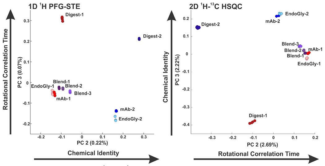
Scoring plots of the 2^nd and 3^rd principal components from PCA on the interlaboratory study dataset from left, 1D ¹H diffusion edited spectra and right, 2D ¹H-¹³C methyl HSQC spectra. For both plots, samples are generally visually differentiated from each other. 1D data are ordered in the 2^ndPC by chemical identity, and in the 3^rd PC by molecular weight, while for the 2D data the converse is true.

When the same analysis is repeated on an expanded set containing data from both 600 MHz spectrometers (Figure S6), samples for the most part remain visually differentiated from one another, but a clear sub-clustering based upon spectrometer is observed for both 1D and 2D datasets. While this suggests, that direct assessment of PCA performed on the full spectral matrix is not robust across instruments, it can be seen that the relative distribution of samples in PC spaces is conserved between instruments. To assess whether these distributions themselves may be a more robust measure for spectral assessments, pairwise Euclidean distances between samples sets were calculated using the respective 2^nd and 3^rd variance-normalized PC coordinates. Variance normalization of PCA scores (eq. 1) was applied to minimize experimental and system-dependent contributions to the observed variance (assuming they are second order with respect to inter-sample variance of interest). As shown in Figure S7A and B and Table S1, results between the two spectrometers are highly similar with average deviations less than 6% for both 1D and 2D datasets, suggesting the variance-normalized Euclidean distance (vNED) may indeed be a robust measure of spectral similarity. Using the vNED, we can further compare the 1D and 2D sets (Figure S7C). Remarkably, while systematic differences are observed as expected, their vNED are highly correlated, with deviation on the order of only 15%. Thus while, potential sources of structural variance (i.e. chemical identity and rotational correlation time) impact 1D and 2D spectra with different sensitivity, leading to differential ordering in the 2^nd and 3^rd PC, iterative decomposition of the data by PCA is able to deconvolute and expose these features for assessment regardless of spectral modality.

Robustness of PC Euclidean Distances

To further investigate the robustness of vNED, a new set of samples was prepared based upon a subset of the samples from the previous example; the two IgG1k mAbs, as well as the papain digest and EndoGly isoform of mAb-1. Data were then recorded on three separate spectrometers at two different fields, with different probe types and variable numbers of scans. To establish a benchmark, data were first acquired at 600 MHz using a room temperature HCN inverse probe with 1024 scans (Table 1, Figure S1). As shown in Figure 3A, all samples cluster by sample type and conform to the expected ordering in the 2^nd and 3^rd PCs established with the previous study data. To determine the applicability of the method to be employed at lower fields, data were then collected at 400 MHz using a room temperature HX inverse probe, with both 512 and 256 scans. While data from different fields cannot be directly assessed together by PCA of the total spectral matrix without sub-clustering by field,²⁵ visual comparison of the distribution of clusters in the 2^nd and 3^rd PC between the 600 MHz (Figure 3A) and 400 MHz data (Figure 3B)reveals a high level of commonality . To more quantitatively assess the similarity of these results, vNED were computed pairwise between the class average positions for both the 256 and 512 scan datasets (Tables S2). As show in Figure 4D, there is a high degree of agreement between both 400 MHz datasets, with deviations less than 3% on average(Q=0.025). Visual assessment of PCA results (Figure 3B) reveals that data cluster by sample class well regardless of number of scans. When the averages of the two 400 MHz datasets are compared to the benchmark 600 MHz dataset (Figure 4B), as slight increase in deviation is observed, but is still less than 5% (Q=0.045), indicating that field effects are negligible and that even with the lower resolution and sensitivity (Table 1, Figure S1), 400 MHz 1D PFG-STE data may still be suitable for HOS characterization when employing a PCA-based approach.

Table 1.

Signal to Noise Values for Experimental Datasets

Dataset	mAb-1	mAb-2	Digest-1	EndoGly-1
400 MHz RT 256 scans	382.09 ± 23.72	344.83 ± 26.55	314.82 ± 12.91	290.20 ± 13.60
400 MHz RT 512 scans	490.36 ± 46.89	482.93 ± 43.41	472.78 ± 15.87	400.21 ± 22.86
600 MHz micro 256 scans	46.58 ± 2.46	39.32 ± 2.78	49.15 ± 4.37	39.25 ± 2.92
600 MHz micro 512 scans	66.08 ± 1.81	54.16 ± 5.15	70.55 ± 3.77	49.1 ± 4.37
600 MHz micro 1024 scans	92.64 ± 7.59	83.44 ± 3.23	97.85 ± 5.05	77.85 ± 1.52
600 MHz RT 1024 scans	768.78 ± 77.59	664.13 ± 27.69	912.97 ± 41.68	693.38 ± 44.69

Sample Tubes†
	298 K	310 K	323 K
600 MHz cryo u5 mm	4472.5 (16.0)‡	2496.5 (8.9) ‡	835.8 (3.0) ‡
600 MHz cryo u4 mm	3972.5 (22.1) ‡	4777.3 (26.5) ‡	5231.6 (29.1) ‡
600 MHz cryo 3 mm	2810.1 (17.6) ‡	3171.5 (19.9) ‡	3910.7 (24.4) ‡

^†mAb-1 only

^‡Replicate data were not acquired to determine uncertainties. Values are normalized to μL of sample in parenthesis

Figure 3.

Scoring plots of the 2^nd and 3^rd principal components from PCA of new data collected on A) 600 MHz RT-TXI probe, 1024 scans, B) 600 MHz RT-TCI microprobe 1024, 512 and 256 scans and C) 400 MHz RT-BBI probe 512 and 256 scans. There is good qualitative agreement in the distribution of sample clusters in PC space between the three spectrometer setups with all spectra clustering by sample and without significant subclustering by number of scans.

Figure 4.

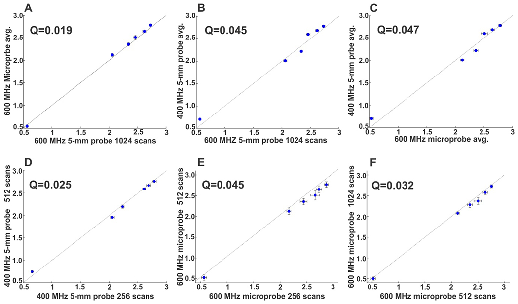
Linear correlation analysis of pairwise variance-normalized PC Euclidean distances (vNED) between sample cluster average positions obtained from the various spectrometer configurations. A) 600 MHz 5 mm probe benchmark set versus 600 MHz Microprobe data averaged over all three sets (256, 512 and 1024 scans). B) 600 MHz 5 mm probe benchmark set versus 400 MHz 5 mm probe data averaged over both sets (2512 and 1024 scans). C) 600 MHz Microprobe data averaged over all three sets versus 400 MHz 5 mm probe data averaged over both sets. D) 400 MHz 5 mm probe 256 scans set versus 400 MHz 5 mm probe 512 scans set. E) 600 MHz Microprobe 256 scans set versus 600 MHz Microprobe 512 scans set. F) 600 MHz Microprobe 512scans set versus 600 MHz Microprobe 1024 scans set. The degree of agreement was assessed by a Q-factor as shown, with the dotted line corresponding to the 1:1 fit.

Clinical formulations of mAbs tend to be at concentrations favorable for NMR analysis (10-100 mg/mL). However, in early development stages, prior to scale-up of manufacture, quantities available for analytical testing may be considerably more limited. Likewise, with the introduction of new modalities such as Bispecific T-Cell Engagers (BiTEs), exhibiting increased potency, lower dosage concentrations are becoming common (1 mg/mL and below).²⁶ To demonstrate the possibility of performing measurement on limited-quantity materials and to test the bounds of sensitivity, 20 μL (800 μg at 40 mg/mL) of each of the test samples was transferred to capillary-NMR tubes and data were acquired on a room temperature HCN inverse 1 mm micro-probe at 600 MHz with a variable number of scans (256, 512, 1024). Although field effects are absent relative to the 600 MHz benchmark data, because of the extreme difference in sample tube and probe architecture, data cannot be compared directly without sub-clustering by probe. However, despite the extremely low S/N (Table 1, Figure S1), as with the 400 MHz data, comparison of the distribution of samples in the 2^nd and 3^rd PC are similar to the benchmark 600 MHz results and do not sub-cluster based upon number of scans (Figure 3C). Indeed, when pairwise vNED are compared between the different microprobe datasets (Figure 4E and 4F), a high degree of correlation is observed, with deviation of less than 5%. We do note the impact of the extremely low S/N of the 256 scan dataset, which results in noticeably large errors in the vNED, and a higher Q-value between the 256-512 (0.045) comparison than the 512-1024 comparison (0.032). Additionally, a slight biasing is observed towards higher vNED for the 256 scan data, still the bias is on the order of the experimental precision (Figure 4E). However, when the average across the datasets (i.e. 1024, 512 and 256 scans) is compared to the benchmark 600 MHz data, a very tight correlation is observed, with deviations less than 2% on average (Figure 4A). Similarly, when compared against the average of the 400 MHz data (Figure 4C), as similar correlation Q-factor is observed as that of the 400 MHz to 600 MHz benchmark data. Taken together this suggests that PCA applied to 1D proton diffusion data substantially eliminates the burden of high S/N relative to PROFILE analysis and enables expanded applications of the method including increased throughput for screening and analysis and for HOS characterization to biopharmaceutical modalities other than mAbs. In particular, it should be stressed that by increasing the sensitivity of the method, it may help to overcome what is often seen as a major limitation of NMR and drive greater adoption of drug product HOS characterization by NMR.

Quantitative Pairwise PCA

In the two examples considered thus far, a different number of sample classes was employed for the analysis of original interlaboratory study data relative to that of the new sample sets. As such, the variance encompassed in the second and third PCs is not consistent between the two analyses and likewise the resulting vNED are not consistent; for example, the Digest 1-mAb 2 distance is ca. 3.65 for the first analysis with nine sample classes and ca. 2.75 for the second analysis with only four classes. As previously reported,¹⁶ the only way to employ PC distances in a rigorously quantitative fashion is to perform PCA on only two sample classes at a time. When this is done, the sample variance can be completely described in the first two principal components (PC1 and PC2). Therefore, to demonstrate the quantitative use of PCA for spectral similarity assessment, we performed pairwise PCA on each of the sample using the 600 MHz microprobe data.

For the vNED analysis, the samples set was both consistent for all PCA examples and contained multiple classes of structural variation. Therefore, it is expected that the inter-sample variation was much greater than the intra-sample, or measurement variation. When pairwise PCA is performed on the same sample set, neither condition is true, with repercussions on how variance normalization should be accomplished. As illustrated in Figure S8, pairwise PCA yields remarkably similar total variation, especially for the second PC, regardless of the nature of the two samples being compared. The magnitude of the intra-sample variation, however, changes considerable, such that a larger variance is observed for highly similar samples while a smaller variance is seen for highly dissimilar samples. Thus, it is necessary to normalize against the measurement variance to obtain meaningful inter-sample distances. In a previous report on pairwise PCA of 2D ¹H-¹³C HSQC data, the measurement variance was estimated from the sum of squares of the total intra-sample variance (eq. 2) for the PCA comparison (i.e. from the two given samples in the pairwise comparison), resulting in a so-called Z-score distance.¹⁶ However, when that measure of variance (internal-self) is employed here, we observe a large scaling in comparison of pairwise distances obtained using 1024, 512 and 256 scans as evidenced by slopes of less than one for linear regression between the 1024 versus 512 scan and 1024 versus 256 scan datasets (Figure 5A, Table S3) Likewise, notable deviations are manifested between the three datasets as indicated by the reduced correlation coefficients from the linear regression between the 1024, 512 and 256 scan datasets (Figure 5B). This suggests that the reproducibility of a 1D PFG-STE experiment on single sample collected five times in series is a poor measure of the true measurement variability of this dataset. In the present case, because data were collected over a wide range of S/N, it might be better to use measure of variance which likewise incorporates a wide range of S/N. To that end, data were reanalyzed using a modified Z-score in which one sample set (mAb-1) was used as an independent variance class (internal-mAb1) such that after the pairwise PCA was performed the variance class was mapped into the resulting PC space and incorporated as a third class in the sum of squares variance normalization (eq. 2). This resulted in an improvement in both the scaling between the microprobe datasets as well as the strength of correlation between them, but significant deviations were still manifested. To more completely probe the measurement variance, three new independent variance sample sets of mAb1 formulated in a different buffer (mab1*, see experimental) were prepared and aliquoted such that one sample was placed into four independent sample tubes, and the second and third independent samples each placed into a single tube. Data were then reanalyzed with serial addition of variance reference sets. As summarized in Figure 5 and Table S3, additional improvements in scaling and correlation between the microprobe datasets are observed for up to two independent tube reference variance sets (External-mAb1* 1 and 2). Addition of a third and fourth independent tube sets gave only minimal improvement in either measure (External-mAb1* 3 and 4). When additional independent sample sets are included further gains are observed for both scaling and correlation, improving with each additional set (External-mAb1* 4+1 and 4+2). Thus, the true measurement variance of this set would seem to include variance from differences in both sample tube (sample height in tube, position of tube in receiver probe, etc.) as well as from non-structural differences in sample composition such as small differences in relative concentration of buffer components.

Figure 5.

Comparison of the effects of different variance reference sets. A) The slope of the best fit linear regression for 1024 vs 512 scan data (blue circles) and 1024 vs 256 scan data (red squares). B) The correlation coefficient for the linear regression of 1024 vs 512 scan data (blue circles) and 1024 vs 256 scan data (red squares). Data were fit such that the intercept was set to zero. C) The percentage overlap of the confidence surfaces between mAb-1 and mAb-1* for 1024 (blue) 512 (red) and 256 (yellow) scan data. The gray area denotes overlap at or below the 95% confidence surface as described in the text.

While increasing the magnitude of variance from the external reference set necessarily dilutes the contributions from the intra-sample variance and thus leads to improved metrics of comparison for the microprobe data sets, it will also, by definition, decrease the inter-sample variance that can be deemed meaningful. To examine the effect of the variance references set on spectral differentiation, we consider the overlap of spectral confidence surfaces (Figure S9). Spectral confidence surfaces can be computed from sample class Z-score distributions as previously described and can serve as a metric for statistically significant class separation.¹⁶ The average overlap was determined between mAb-1 and the mAb-1* samples (Figure 5C, Table S3). For all three microprobe datasets, virtually no overlap was observed between mAb-1 and mAb-1* when variance was measured directly from intra-sample variance (Internal-Self). When the Internal-mAb1 variance class was employed, a small degree of overlap (1-3%) was observed in the 256 and 512 scan datasets, but not in the 1024 scan dataset. With the use of the External-mAb1* variance classes, increases in overlap were observed for the addition of the first two sample tubes (External-mAb1* 1 and 2) and then plateaued for the additional third and fourth tubes (External-mAb1* 3 and 4), with increases most notable on the 256 and 512 scan sets. Inclusion of the additional independent samples (External-mAb1* 4+1 and 4+2) resulted in further increases in overlap, with gains most substantial on the 512 and 1024 scan sets (Figure 5C).

This raises the question as to what constitutes a statistically significant cluster separation, or what the minimum distance at which two cluster might be deemed statistically different is. Although that specification will ultimately be governed in the context of a specific system and given application, we consider here the case where an overlap at the 95% confidence surface is the cutoff. To establish upper bounds for the cutoff criteria, we first estimate from the case where two clusters each with identical spread in PC1 and PC2 (i.e. having circular confidence surfaces) are separated from one another in one dimension only such that their 95% confidence surfaces touch. By definition, this will be at an inter-cluster distance of approximately 4σ and will give rise to an overlap of 9%. However, the true relationship between degree of overlap as well as the inter-sample distance is complex, depending on sample distributions in both PC1 and PC2 as well as the angle between sample centers and the PC coordinate normal. Indeed, when the correlation between sample distance and degree of overlap is plotted, we find that the data follow a broader trend resulting in greater overlap at larger distances (Figure S10) and we also observe overlap of the 95% confidence surface at distance of 9σ and overlap of 3.9% (Figure S9). Notably, using these values as a cutoff implies that for the lowest, 256 scan set, mAb1 and mAb1* are not statistically differentiated once an external variance reference is employed, while for the highest, 1024 scan, set, the samples remain differentiated even when using the greatest variance set (External-mAb1* 4+2). Thus, while limitations of S/N have been greatly ameliorated by PROFOUND, minimum thresholds should still be considered within the context of specific sample differences, inherent measurement variation and degree of statistical rigor desired, which in the present application would be greater than ca. 50:1.

Effects of Sample Tube on Experimental S/N

A major limitation of employing the diffusion edited PFG-STE experiment is the need to use 4 mm susceptibility matched symmetric microtubes. In addition to being of limited commercial availability, they are less ideal for a variety of other NMR experiment, the 2D ¹H-¹³C methyl HSQC chief among them. The use of 4 mm microtubes has been recommended due to the superior properties of narrow radius tubes and susceptibility matched symmetric microtubes in minimizing Rayleigh-Benard convection,^27,28 thus maximizing sensitivity of the PFG-STE experiment. As we have demonstrated here that we can tolerate considerable experimental noise and still achieve reasonable results by PROFOUND, this limitation may no longer be necessary. To assess the relative performance of other NMR tube architectures, PFG-STE spectra of the mAb-1 sample were recorded at 600 MHz with an inverse HCN TCI cryoprobe with 1024 scans in three different NMR tubes; a 5 mm microtube, a 4 mm microtube and a standard 3 mm tube. For each tube data were collected at 298 K, 310 K and 323 K. Results are summarized in Table 1 and Figure 6. On an absolute basis (Figure 6A), at 298 K we find the 5 mm microtube performs best, followed by the 4 mm microtube then the 3 mm standard tube. However, at this temperature, on a per volume basis (Figure 6B), we observe that all tubes perform similarly, suggesting that convections effects are minimal. At 310 K, convection differences in tubes become manifested, with the 4 mm microtube performing slightly better than the 3 mm on a per volume basis, but with the 5 mm microtube performing considerably worse. Still, with S/N of approximately half of the 4 mm microtube, the 5 mm microtube should still be adequate for many applications. At 323 K, the 4 mm microtube again perform slightly better than the 3 mm microtube on a per volume basis. The 5 mm microtube however drops to just 17 % of the S/N of the 4 mm microtube. While the absolute S/N of the 5 mm microtube at 323 K should be adequate for PROFOUND applications, given the far superior performance of the 4 mm and 3 mm microtubes under these conditions their use is still advisable if practical.

Figure 6.

S/N of mAb1-1 1d ¹H diffusion edited PFG-STE spectra as a function of sample tube architecture and temperature. A) Relative S/N normalized to the maximum S/N of the dataset from a 4 mm microtube (μ4 mm) at 323 K. B) Relative S/N normalized to sample tube volume (300 μL, 180 μL and 160 μL for μ5 mm, μ4 mm and 3 mm respectively) and maximum S/N of the dataset.

Conclusion

We have introduced the new PROFOUND method, which is based on the quantitative pairwise PCA previously demonstrated on 2D ¹H-¹³C HSQC spectra and the 1D proton PROFILE method. The 1D proton PROFILE method has been instrumental in establishing fit-for-purpose of NMR for HOS characterization of protein therapeutics including mAbs. However, the PROFILE method has analytical deficiencies, most notably its dependence on linear correlation analysis and the accompanying requirement for high experimental signal to noise. By preserving the core strengths of PROFILE, PROFOUND overcomes the limitations of PROFILE using a multivariate data analysis approach based on PCA with quantitative distance analysis We have demonstrated here that results from PROFOUND analysis are robust with respect to instrument and operator, are tolerant to high experimental noise and that comparable results can be achieved even when moving to lower field strengths with less resolved spectra. As such, the method can potentially be extended to samples of limited quantity, either in absolute terms or in relative concentration and be employed in situations where mid-to-high field spectrometers are not available. Additionally, for typical sample conditions run at fields of 600 MHz or greater, data can be readily acquired in minutes-to hours instead of several hours. By increasing throughput of the 1D method, it can better serve as a primary screening technique to guide the deployment of the more demanding but information rich 2D technique to truly make NMR a multi-modal tool for HOS characterization. Indeed, the complementarity of the 1D and 2D method were further confirmed in this study. Results of PCA on a common set of samples revealed very similar results between the two modalities, suggesting information content is largely preserved in both. While the 1D method has been proven to be more sensitive to chemical identity and the 2D to rotational correlation time, the multidimensional nature of PCA ensures both aspects are adequately captured by each method, albeit with opposite sensitivities and corresponding orders of ranking in PC space. As such, multi-modal NMR characterization of biotherapeutics should be considered as fit-for-purpose dictates. Furthermore, we expect that the spectral decomposition and distance analysis at the core of PROFOUND may find applicability in other spectroscopic modalities and serve as a general method to improve the quantitative characterization of HOS.

Abbreviations:

BiTEs

Bispecific T-Cell Engagers

CD

Circular dichroism

FTIR

Fourier transform infrared spectroscopy

HSQC

Heteronuclear single-quantum correlation spectroscopy

HOS

Higher order structure

mAb

Monoclonal antibody

NIPALS

Nonlinear Iterative Partial Least Squares

1D

One-dimensional

PTM

Post translational modifications

PCA

Principal component analysis

PC

Principal component

PROFILE

Protein Fingerprint by Lineshape Enhancement

PROFOUND

Protein Fingerprinting obtained using NIPALS Decomposition

PFG-STE

Pulsed field gradient stimulated echo

S/N

Signal to noise

vNED

Variance-normalized Euclidean distance

References

- 1.Chen K, Long DS, Lute SC, Levy MJ, Brorson KA, Keire DA. Simple NMR methods for evaluating higher order structures of monoclonal antibody therapeutics with quinary structure. J Pharm Biomed Anal 2016;128:398–407. [DOI] [PMC free article] [PubMed] [Google Scholar]
- 2.Poppe L, Jordan JB, Lawson K, Jerums M, Apostol I, Schnier PD. Profiling Formulated Monoclonal Antibodies by 1H NMR Spectroscopy. Anal Chem 2013;85(20):9623–9629. [DOI] [PubMed] [Google Scholar]
- 3.Franks J, Glushka JN, Jones MT, Live DH, Zou Q, Prestegard JH. Spin Diffusion Editing for Structural Fingerprints of Therapeutic Antibodies. Anal Chem 2016;88(2):1320–1327. [DOI] [PMC free article] [PubMed] [Google Scholar]
- 4.Aubin Y, Freedberg DI, Keire DA. One- and Two-Dimensional NMR Techniques for Biopharmaceuticals. In: Houde DJ, Berkowitz SA, eds. Biophysical Characterization of Proteins in Developing Biopharmaceuticals. Elsevier; 2015:341–383. [Google Scholar]
- 5.Poppe L, Jordan JB, Rogers G, Schnier PD. On the Analytical Superiority of 1D NMR for Fingerprinting the Higher Order Structure of Protein Therapeutics Compared to Multidimensional NMR Methods. Anal Chem 2015;87(11):5539–5545. [DOI] [PubMed] [Google Scholar]
- 6.Casagrande F, Dégardin K, Ross A. Protein NMR of biologicals: analytical support for development and marketed products. J Biomol NMR 2020;74(10-11):657–671. [DOI] [PubMed] [Google Scholar]
- 7.Wang D, Park J, Patil SM, et al. An NMR-Based Similarity Metric for Higher Order Structure Quality Assessment Among U.S. Marketed Insulin Therapeutics. J Pharm Sci 2020;109(4):1519–1528. [DOI] [PubMed] [Google Scholar]
- 8.Bramham JE, Podmore A, Davies SA, Golovanov AP. Comprehensive Assessment of Protein and Excipient Stability in Biopharmaceutical Formulations Using 1 H NMR Spectroscopy. ACS Pharmacol Transl Sci 2021;4(1):288–295. [DOI] [PMC free article] [PubMed] [Google Scholar]
- 9.Wen J, Batabyal D, Knutson N, Lord H, Wikström M. A Comparison Between Emerging and Current Biophysical Methods for the Assessment of Higher-Order Structure of Biopharmaceuticals. J Pharm Sci 2020;109(1):247–253. [DOI] [PubMed] [Google Scholar]
- 10.Elliott KW, Ghasriani H, Wikström M, et al. Comparative Analysis of One-Dimensional Protein Fingerprint by Line Shape Enhancement and Two-Dimensional 1 H, 13 C Methyl NMR Methods for Characterization of the Higher Order Structure of IgG1 Monoclonal Antibodies. Anal Chem 2020;92(9):6366–6373. [DOI] [PMC free article] [PubMed] [Google Scholar]
- 11.Arbogast LW, Brinson RG, Marino JP. Mapping Monoclonal Antibody Structure by 2D 13 C NMR at Natural Abundance. Anal Chem 2015;87(7):3556–3561. [DOI] [PubMed] [Google Scholar]
- 12.Arbogast LW, Delaglio F, Schiel JE, Marino JP. Multivariate Analysis of Two-Dimensional 1 H, 13 C Methyl NMR Spectra of Monoclonal Antibody Therapeutics To Facilitate Assessment of Higher Order Structure. Anal Chem 2017;89(21):11839–11845. [DOI] [PMC free article] [PubMed] [Google Scholar]
- 13.Arbogast LW, Brinson RG, Formolo T, Hoopes JT, Marino JP. 2D 1HN, 15N Correlated NMR Methods at Natural Abundance for Obtaining Structural Maps and Statistical Comparability of Monoclonal Antibodies. Pharm Res 2016;33(2):462–475. [DOI] [PubMed] [Google Scholar]
- 14.Mckay RT. How the 1D-NOESY suppresses solvent signal in metabonomics NMR spectroscopy: An examination of the pulse sequence components and evolution. Concepts Magn Reson Part A 2011;38A(5):197–220. [Google Scholar]
- 15.Wold H Nonlinear Estimation by Iterative Least Square Procedures. In: David FN, ed. Research Papers in Statistics. John Wiley & Sons, Inc.; 1966:411–444. [Google Scholar]
- 16.Brinson RG, Elliott KW, Arbogast LW, et al. Principal component analysis for automated classification of 2D spectra and interferograms of protein therapeutics: influence of noise, reconstruction details, and data preparation. J Biomol NMR 2020;74(10-11):643–656. [DOI] [PubMed] [Google Scholar]
- 17.Delaglio F, Grzesiek S, Vuister G, Zhu G, Pfeifer J, Bax A. NMRPipe: A multidimensional spectral processing system based on UNIX pipes. J Biomol NMR 1995;6(3):277–293. [DOI] [PubMed] [Google Scholar]
- 18.Johnson BA, Blevins RA. NMR View: A computer program for the visualization and analysis of NMR data. J Biomol NMR 1994;4(5):603–614. [DOI] [PubMed] [Google Scholar]
- 19.Ousterhout JK. TCL and the Tk Toolkit. Published online 1994
- 20. https://www.ibbr.umd.edu/nmrpipe/install.html.
- 21.Maciejewski MW, Schuyler AD, Gryk MR, et al. NMRbox: A Resource for Biomolecular NMR Computation. Biophys J 2017;112(8):1529–1534. [DOI] [PMC free article] [PubMed] [Google Scholar]
- 22.Cornilescu G, Marquardt JL, Ottiger M, Bax A. Validation of Protein Structure from Anisotropic Carbonyl Chemical Shifts in a Dilute Liquid Crystalline Phase. J Am Chem Soc 1998;120(27):6836–6837. [Google Scholar]
- 23.Arbogast LW, Delaglio F, Brinson RG, Marino JP. Assessment of the Higher-Order Structure of Formulated Monoclonal Antibody Therapeutics by 2D Methyl Correlated NMR and Principal Component Analysis. Curr Protoc Protein Sci 2020;100(1):105. [DOI] [PMC free article] [PubMed] [Google Scholar]
- 24.Campbell I, Dobson C, Williams RJ, Xavier A. Resolution enhancement of protein PMR spectra using the difference between a broadened and a normal spectrum. J Magn Reson 1973;11(2):172–181. [Google Scholar]
- 25.Brinson RG, Arbogast LW, Marino JP, Delaglio F. Best Practices in Utilization of 2D-NMR Spectral Data as the Input for Chemometric Analysis in Biopharmaceutical Applications. J Chem Inf Model 2020;60(4):2339–2355. [DOI] [PubMed] [Google Scholar]
- 26.Goebeler M-E, Bargou RC. T cell-engaging therapies — BiTEs and beyond. Nat Rev Clin Oncol 2020;17(7):418–434. [DOI] [PubMed] [Google Scholar]
- 27.Goux WJ, Verkruyse LA, Saltert SJ. The impact of Rayleigh-Benard convection on NMR pulsed-field-gradient diffusion measurements. J Magn Reson 1990;88(3):609–614. [Google Scholar]
- 28.Swan I, Reid M, Howe PWA, et al. Sample convection in liquid-state NMR: Why it is always with us, and what we can do about it. J Magn Reson 2015;252:120–129. [DOI] [PubMed] [Google Scholar]
Associated Data
This section collects any data citations, data availability statements, or supplementary materials included in this article.