Clustering and dynamic recognition based auto-reservoir neural network: A wait-and-see approach for short-term park power load forecasting

Summary

This paper proposes a novel clustering and dynamic recognition–based auto-reservoir neural network (CDbARNN) for short-term load forecasting (STLF) of industrial park microgrids. In CDbARNN, the available load sets are first decomposed into several clusters via K-means clustering. Then, by extracting characteristic information of the load series input to CDbARNN and the load curves belonging to each cluster center, a dynamic recognition technology is developed to identify which cluster of the input load series belongs to. After that, the input load series and the load curves of the cluster to which it belongs constitute a short-term high-dimensional matrix entered into the reservoir of CDbARNN. Finally, reservoir node numbers of CDbARNN which are used to match different clusters are optimized. Numerical experiments conducted on STLF of an actual industrial park microgrid indicate the dominating performance of the proposed approach through several cases and comparisons with other well-known deep learning methods.

Graphical abstract

Highlights

• •A CDbARNN-based model-free method was developed for multistep-ahead forecasting
• •K-means clustering was presented to decompose the load data fed into CDbARNN
• •The reservoir nodes of CDbARNN were optimized to enhance forecasting accuracy
• •Dynamic recognition technique was utilized in CDbARNN to investigate load curves

Engineering; Electrical engineering; Energy engineering; Energy systems; Mechanical engineering

Introduction

Motivation

Short-term load forecasting (STLF) has garnered significant attention in the context of the modernization of industrial parks.^1,2 Accurate STLF plays a crucial role in facilitating the resolution of the power supply–demand imbalance. Additionally, it aids in formulating power purchase plans and supports the analysis of energy storage system operation strategies to realize the economic operation of the parks.^3,4,5 However, the increasing integration of various electrical devices, coupled with various factors such as power demand, weather conditions, regional characteristics, and temperature has exacerbated the stochastic fluctuations in the load curve of industrial parks, posing substantial challenges for STLF.^6,7 In light of these challenges, this paper proposes a novel model to address the short-term power load forecasting problem and effectively capture the complex dynamics associated with various electricity consumption behaviors, alongside other significant factors.

Literature survey

In recent years, the development of mathematical theory and modern computational technology boost continuous improvement of load forecasting models, therefore, varieties of models have been advocated for practical applications. There are, generally speaking, three categories of forecasting models, i.e., classical forecasting models, modern forecasting models, and hybrid models.¹

One representative of classical forecasting models is the Kalman filter method. For example, Sharma et al. proposed a blind Kalman filtering algorithm for STLF and applied it both on load profile estimation and peak load forecast.⁸ The Kalman filtering obtains the best estimate of the state of the system at one time by filtering the sample data and uses the new data obtained to forecast the future state.⁹ The disadvantage is that it is difficult to accurately estimate the statistical characteristics of system noise in applications. If the load forecasting model is built on the basis of inaccurate model parameters and noise statistics, a large forecasting error will occur.¹⁰ Another widely used classical forecasting model is the time series method. The disadvantage is that it has high requirements for the stationarity of the time series of the data, and it focuses too much on the fitting of the data and ignores the variability of the data.¹¹ With the modification of the power grid structure, the complexity and fluctuation of the power load in industrial parks are increasing. Although the classical forecasting model has a fast calculation speed, its simple structure prevents it from adapting to changes in load trends.¹²

In the context that a forecasting model with assertive stochastic and non-linear behavior capturing abilities is needed, AI models have been utilized commonly,¹³ including artificial neural network (ANN), support vector regression (SVR), fuzzy logic approach, etc. Kamran et al. designed an ANN based on artificial bee colony algorithm and applied it to the Bushehr Province demand forecasting.¹⁴ Yang et al. proposed a sequential grid approach based SVR model for STLF by introducing the asymptotic normality of a fixed grid point of parameters.¹⁵ The latest short-term but high-dimensional data possess rich information on its immediate future evolution than the remote-past time series, which is more useful for the power load forecasting.^16,17 With respect to hybrid models, recent research has primarily focused on combining AI methods with a variety of techniques to leverage the combined advantages of individual models. For instance, Hafeez et al. integrated a locally weighted SVR based forecaster with adaptive grasshopper optimization and feature engineering to address the challenges of parameter tuning and computational complexity, and they demonstrated its effectiveness using real half-hourly load data from five states of Australia.¹⁷ Jiang et al. introduced a framework combing long short-term memory and convolutional neural network, which learns the recent electricity usage behavior and features in the low-level information extraction stage and then integrates the forecasting information in the high-level stage.¹⁸ But, in general, the above-mentioned models tend to be data-hungry, requiring long observation times and substantial computational resources.¹⁹ So, due to the insufficient data, it is a challenging task to make multistep-ahead forecasting based only on short-term load series. Furthermore, even if AI is compelled to perform STLF, it will be vulnerable to local optima and overfitting.¹⁷

In order to resolve the above limitations, Chen et al. proposed an auto-reservoir neural network (ARNN) by combining reservoir computing (RC) and spatiotemporal information (STI) transformation.²⁰ ARNN is a variant of neural networks recently developed following RC frameworks that is suitable for temporal and sequential information processing. It achieves an accurate, robust, and computationally efficient multistep-ahead forecasting with short-term high-dimensional data.²⁰ Unlike traditional RC, which uses an external dynamical system unrelated to the target system as its reservoir,^21,22,23 ARNN uses the observed high-dimensional information as its reservoir, which uses STI to map high-dimensional data to future temporal values of a target variable. It has been put into practical application; for instance, Li et al. proposed a method to forecast outbreaks of Covid-19, called the landscape network entropy based ARNN.²⁴

In the past few years, ARNN has achieved great success in learning the dynamics of time series and demonstrated accuracy in forecasting gently changing data.^20,25,26 But it faces challenges when dealing with data mutations caused by external factors in real-life scenarios. To address this issue, wavelet transform and empirical mode decomposition (EMD) have been commonly used in previous studies to decompose and simplify the original load series. For instance, Gao et al. employed empirical wavelet transformation in a walk-forward approach, decomposing the raw load data into sub-series that were fed into the neural network for prediction.²⁷ Similarly, Liang et al. proposed a hybrid model, EMD-mRMR-FOA-GRNN, which utilized EMD to decompose nonstationary load series into bivariate modal components to enhance prediction precision.¹ However, predicting all deconstructed components simultaneously in these models increases their complexity and computational cost, leading to potential errors in ensemble forecasting.³

In contrast, ARNN is specifically designed for forecasting high-dimensional data. However, when the dimensions of the data are not sufficiently high, ARNN may not effectively highlight its advantages over other forecasting models.²⁰ In the historical daily load data of industrial park microgrids, there are often significant similarities that can be extracted. For example, the electricity consumption trend on holidays or days with similar weather conditions tends to exhibit similarities.^28,29,30 By leveraging the similarities in load series, we can compensate for the limitations of ARNN in handling load mutations by forming them into a high-dimensional input dataset.

Previous studies have employed various characteristic variables such as meteorological data, date types, and electricity prices to identify similar load days.^31,32 However, the consideration of numerous characteristic factors and the intricate relationships between vectors pose challenges. Therefore, identifying similar load series in a simple and effective manner to drive ARNN for achieving more accurate STLF remains to be studied.

Contributions

To address the above-mentioned limitations of ARNN, this study proposes a clustering and dynamic recognition (DR) based ARNN (CDbARNN) for STLF. The CDbARNN is a wait-and-see approach, which consists of four steps, i.e., decomposition, recognition, reconstruction, and forecasting.

The main contributions of this study can be outlined as follows.

• (1)Introducing the CDbARNN into an STLF model for the first time achieves a model-free method to make multistep-ahead forecasting.
• (2)Inspired by the concept of “Birds of a Feather Flock Together”, we introduce the K-means clustering algorithm to decompose the load data fed into CDbARNN. This approach effectively extracts and identifies the fluctuation characteristics of the data, contributing to more accurate forecasting.
• (3)The reservoir nodes of CDbARNN applied to different clusters are optimized to enhance forecasting accuracy and stability simultaneously. This optimization process improves the performance of the model by adapting to the specific characteristics of different load clusters.
• (4)The DR technique is utilized in CDbARNN to determine which cluster the input load data for forecasting belongs to. This enables the model to capture internal features and reconstruct the input matrix, facilitating more precise forecasting within each cluster.

Results and discussion

Data description and pre-processing

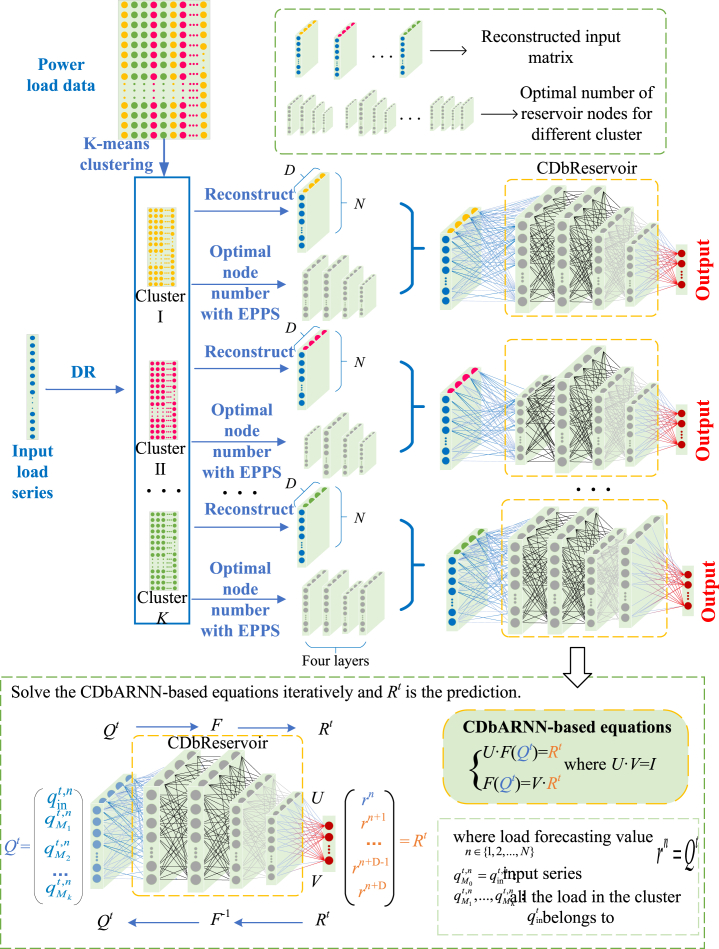
To evaluate the forecasting performance of CDbARNN, this study conducts an empirical study on an industrial park in Zibo city, China. The load data is collected at a frequency of one observation per minute, resulting in a total of 1,440 data points per day. The historical load data spans 365 days, resulting in a total of 365 rows of daily data. As depicted in Figure 15, the CDbARNN framework directly transforms the observed high-dimensional dynamic information, denoted as matrix $Q^t={\left(q_{\text{in}}^{t,n},q_{M_1}^{t,n},q_{M_2}^{t,n},\dots ,q_{M_k}^{t,n}\right)}^{\prime },n=\mathrm{1,2},\dots ,N$, into the reservoir and maps the high-dimensional spatial data to a one-dimensional delay time vector denoted as vector $R^t={\left(r^n,r^{n+1},\dots ,r^{n+D-1},r^{n+D}\right)}^{\prime }$. In the training phase, the length of vector $N$ is used for training, and the length of vector $D$ is used for prediction.

Figure 15.

The flow chart of CDbARNN.

Evaluation metrics

To scientifically and systematically evaluate the performance of our proposed approach, the following four evaluation criteria are used in this study, i.e., normalized mean absolute error (NMAE), normalized root-mean-square error (NRMSE), mean absolute percentage error (MAPE), and Willmott index of agreement (IA).

$$\text{NMAE}=\frac{1}{\text{NUM}}\sum _{t=1}^{\text{NUM}}\frac{\left|x_t-y_t\right|}{\max \left\{x_t\right\}}\times 100\%$$ (Equation 1a)

$$\text{NRMSE}=\frac{1}{\max \left\{x_t\right\}}\sqrt{\frac{1}{\text{NUM}}\sum _{t=1}^{\text{NUM}}{\left(x_t-y_t\right)}^2}\times 100\%$$ (Equation 1b)

$$\text{MAPE}=\frac{1}{\text{NUM}}\sum _{t=1}^{\text{NUM}}\frac{\left|x_t-y_t\right|}{x_t}\times 100\%$$ (Equation 1c)

$$\text{IA}=1-\frac{\sum _{t=1}^{\text{NUM}}{\left(x_t-y_t\right)}^2}{\sum _{t=1}^{\text{NUM}}{\left(\left|y_t-{\overline{x}}_t\right|+\left|x_t-{\overline{x}}_t\right|\right)}^2}$$ (Equation 1d)

where NUM = 1440, $x_t$ is the true load series, $y_t$ is the forecasting load series, ${\overline{x}}_t$ is the average value of the true load series and $\max \left\{x_t\right\}$ is the maximum value of the true load series. Among these four indicators, the smaller the value of NMAE, NRMSE, or MAPE, the more accurate or stable the forecasting result is. Here, NMAE is used to measure the forecasting accuracy and is expressed as a percentage, ranging from 0 to 100%. A smaller NMAE indicates higher forecasting accuracy, while an NMAE of zero indicates a perfect model. NMAE provides a superior measure of forecasting accuracy as it avoids scale dependency, allowing for fair comparisons between different models regardless of the magnitude of the data.³³ NRMSE, on the other hand, overcomes scale dependence and simplifies the comparison between models that have different scales or datasets. By normalizing the RMSE values, NRMSE enables a standardized measure of forecast accuracy, facilitating meaningful comparisons across different models.^34,35 IA is a standardized measure of the degree of forecasting error of the model and it only takes values between zero and one. The closer the forecasting value matches the actual value the closer IA is to 1.

Analysis of forecasting results

Comparison with ARNN

In this part, comparative simulations are conducted to validate the effectiveness of CDbARNN. Specifically, we compare performances of CDbARNN, CDbARNN without node number optimization (CDbARNNwNNO), and ARNN on load forecasting under two scenarios. In Scenario 1, three load curves are randomly selected from Clusters I to III, while in Scenario 2, three load curves are randomly generated from Clusters I to III. Another is to forecast after randomly generating a load curve based on the three cluster centers. Evaluations are conducted on four indexes, i.e., MAPE, NMAE, NRMSE, and IA, and results are shown in Table 1. It lists the detailed forecasting results of different methods under different scenarios. The forecasting error is the average value of all load curve errors in each cluster. It shows that the proposed CDbARNN has the most prominent forecasting performance, as indicated by the approximately 1.09%, 1.84% and 7.49% lower NMAE, NRMSE, and MAPE, and 0.05 higher IA, respectively, when compared with ARNN in Scenario 1. And in Scenario 2, it is indicated by the approximately 1.36%, 1.72% and 7.22% lower NMAE, NRMSE, and MAPE, and 0.03 higher IA. The enhancement of forecasting accuracy could be attributed to K-means clustering and DR. With these strategies, the input matrix is reconstructed and obtains the optimal node numbers. In this way, the data similarity characteristic information drives the input load series to realize STLF directly in the cluster it belongs to, that we can use more sufficient information to improve the forecasting precision.

Table 1.

Performance evaluation of CDbARNN on industrial park load forecasting

Evaluation metrics	Forecasting method	Scenario 1			Scenario 2
		I	II	III	I	II	III
NMAE(%)	ARNN	4.12	6.18	6.13	14.72	16.21	19.70
	CDbARNNwNNO	4.10	4.15	5.44	11.46	16.13	19.54
	CDbARNN	3.86	3.98	5.33	11.44	16.11	19.01
NRMSE(%)	ARNN	6.47	9.26	9.17	18.72	20.11	23.84
	CDbARNNwNNO	6.21	5.95	7.83	17.32	19.97	23.71
	CDbARNN	5.87	5.83	7.67	14.47	19.83	23.20
MAPE(%)	ARNN	18.54	21.35	20.74	60.33	72.80	83.61
	CDbARNNwNNO	14.28	11.93	15.10	59.04	71.63	79.15
	CDbARNN	11.67	11.71	14.78	54.75	66.98	73.36
IA	ARNN	0.95	0.92	0.88	0.69	0.58	0.38
	CDbARNNwNNO	0.97	0.96	0.89	0.69	0.60	0.41
	CDbARNN	0.98	0.98	0.93	0.69	0.62	0.42

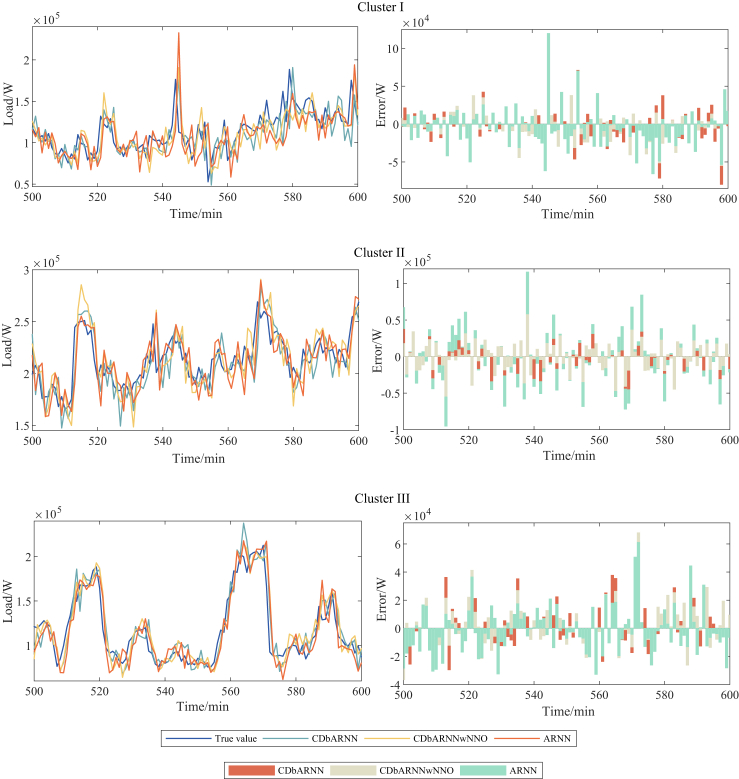
Besides, the forecasting performance of the proposed CDbARNN under Scenario 1 is depicted by Figure 1. We choose the most representative three days from each of the three clusters to illustrate the effectiveness. It shows the forecasting results and errors from the 500th minute to the 600th minute on the three days, which is the time segment of a day when work begins. The left column is the comparison between the forecasting value and the true value, and the right column is the error of the true value minus the forecasting value. It can be seen from Figure 1 that the forecasting value obtained by the proposed CDbARNN method has the trend closest to the true value, that is, the forecasting method has the strongest ability to track the true value. Although ARNN has an accurate short-term forecasting, its high-dimensional input matrix containing information independent of the target variable makes it less effective than CDbARNN. As for CDbARNNwNNO, no matter which cluster of loads is forecasted, its reservoir node is same. Without the optimization node number, it doesn’t work as well as CDbARNN. Furthermore, we observe that the error of Cluster III changes little. The main reason is that the load curves in Cluster III are holidays, with a low power consumption and small fluctuation range, so the forecasting superiority of the proposed CDbARNN is not obvious. Clusters I and II correspond to working days, with a large fluctuation range, which can better reflect the advantages of CDbARNN for STLF.

Figure 1.

Comparison of forecasting performance among CDbARNN, CDbARNNwNNO and ARNN in three clusters.

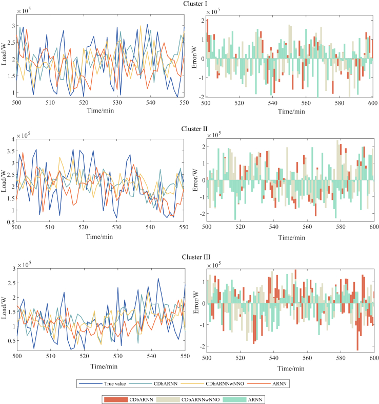
Moreover, the forecasting performance of the proposed CDbARNN under Scenario 2 is depicted by Figure 2. Visually inspecting the left column of the figure, CDbARNN can effectively capture the basic trends in the short-term load profile with more subtle and various random noise. The right column of Figure 2 illustrates the comparison of the forecasting error of different methods represented with bars.

Figure 2.

Comparison of forecasting performance among CDbARNN, CDbARNNwNNO and ARNN in curves randomly generated.

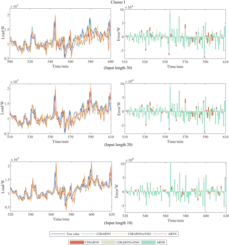
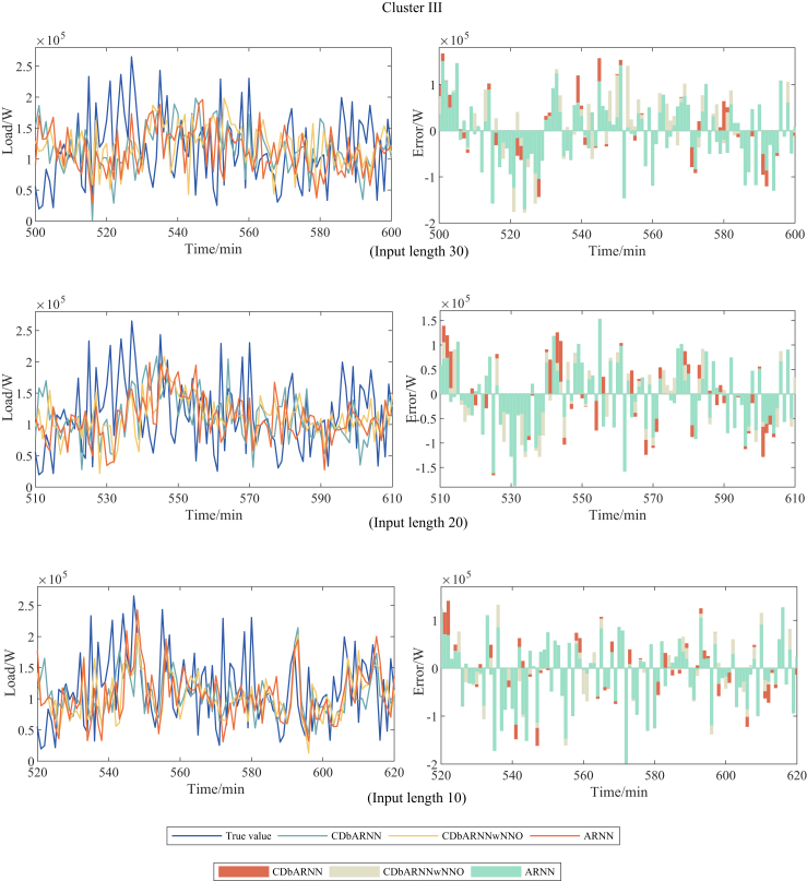
To verify the algorithm’s dependence on the length of the input series, Table 2 shows the forecasting performance of CDbARNN on 30, 20 and 10 input load series lengths. The performance of CDbARNN also dominates when compared with various forecasting methods on different input load series lengths. When the input lengths are 30, 20, and 10, the NMAE of CDbARNN are approximately 0.22%, 0.28%, 0.32% lower than ARNN, and the MAPE of CDbARNN are approximately 1.32%, 1.82%, 1.14% lower, validating its effectiveness. The NRMAE of CDbARNN are approximately 0.33%, 0.39%, 0.44% lower than ARNN, and the IA of CDbARNN are approximately 0.015%, 0.018%, 0.02% higher, further validating its better stability. Furthermore, the decrease of input load series length does not affect the performance of CDbARNN in terms of MAPE, NMAE, and NRMSE. This demonstrates that CDbARNN, in contrast to traditional neural networks, doesn’t require a massive amount of data to train and has excellent computational efficiency, opening up a new avenue for STLF.

Table 2.

Performance evaluation of CDbARNN on different lengths of input load series

Input length	Evaluation metric	Forecasting method	Scenario 1			Scenario 2
			I	II	III	I	I	III
30	NMAE (%)	ARNN	4.89	3.48	5.06	14.76	16.39	20.00
		CDbARNNwNNO	4.78	3.35	4.99	14.57	16.32	19.64
		CDbARNN	4.66	3.34	4.94	14.42	16.27	19.63
	NRMSE (%)	ARNN	7.83	4.80	6.90	18.73	20.16	24.30
		CDbARNNwNNO	7.39	4.67	6.81	18.46	20.12	23.92
		CDbARNN	7.26	4.65	6.78	18.30	20.02	23.75
	MAPE (%)	ARNN	13.31	10.47	14.36	59.98	75.04	80.49
		CDbARNNwNNO	12.97	10.19	14.24	58.46	74.31	78.80
		CDbARNN	12.49	10.12	14.19	56.43	73.81	78.68
	IA	ARNN	0.95	0.97	0.96	0.68	0.57	0.39
		CDbARNNwNNO	0.95	0.99	0.96	0.69	0.58	0.40
		CDbARNN	0.96	0.99	0.97	0.69	0.59	0.42
20	NMAE (%)	ARNN	4.75	3.46	4.82	14.51	16.42	19.82
		CDbARNNwNNO	4.64	3.38	4.59	14.31	15.98	19.76
		CDbARNN	4.54	3.35	4.58	14.03	15.89	19.69
	NRMSE (%)	ARNN	7.58	4.75	6.71	18.42	20.20	24.16
		CDbARNNwNNO	7.25	4.70	6.50	18.05	19.64	24.06
		CDbARNN	7.21	4.63	6.40	17.75	19.48	23.94
	MAPE (%)	ARNN	12.61	10.47	13.59	55.69	72.12	77.01
		CDbARNNwNNO	12.30	10.24	13.07	55.06	70.13	76.96
		CDbARNN	12.14	10.22	12.79	53.69	66.86	74.85
	IA	ARNN	0.95	0.99	0.96	0.68	0.57	0.38
		CDbARNNwNNO	0.96	0.99	0.97	0.70	0.59	0.40
		CDbARNN	0.96	0.99	0.97	0.71	0.60	0.41
10	NMAE (%)	ARNN	4.49	3.18	4.48	15.28	16.93	20.33
		CDbARNNwNNO	4.46	3.15	4.43	14.68	16.81	20.18
		CDbARNN	4.37	3.14	4.42	14.59	16.56	19.71
	NRMSE (%)	ARNN	7.15	4.55	6.40	19.58	20.97	24.92
		CDbARNNwNNO	7.14	4.53	6.34	18.57	20.83	24.75
		CDbARNN	6.97	4.49	6.31	18.55	20.37	24.26
	MAPE (%)	ARNN	11.98	9.52	12.56	55.47	69.77	75.60
		CDbARNNwNNO	11.81	9.44	12.47	54.79	69.52	74.58
		CDbARNN	11.58	9.31	12.46	54.57	69.37	70.76
	IA	ARNN	0.96	0.99	0.96	0.66	0.56	0.42
		CDbARNNwNNO	0.96	0.99	0.97	0.69	0.57	0.43
		CDbARNN	0.97	0.99	0.97	0.70	0.59	0.45

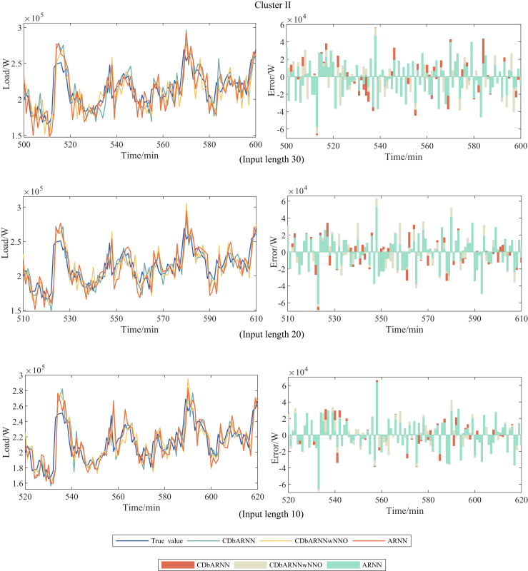
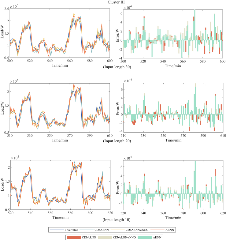
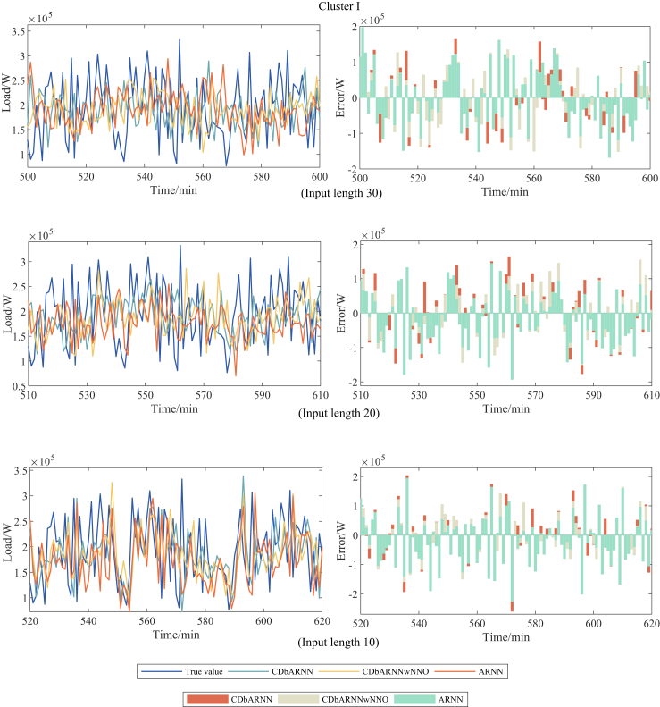
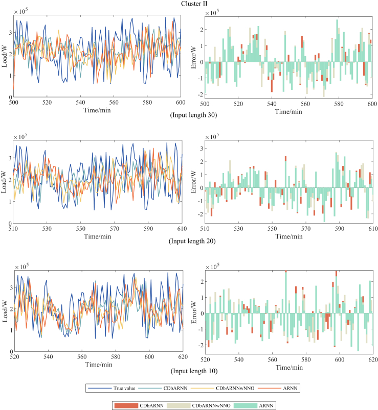
Moreover, the forecasting performance of the proposed CDbARNN under different input length in Scenarios 1 and 2 is depicted by Figures 3, 4, 5, 6, 7, and 8.

Figure 3.

Comparison of forecasting performance among CDbARNN, CDbARNNwNNO and ARNN on different input lengths under Scenario 1, Cluster I.

Figure 4.

Comparison of forecasting performance among CDbARNN, CDbARNNwNNO and ARNN on different input lengths under Scenario 1, Cluster II.

Figure 5.

Comparison of forecasting performance among CDbARNN, CDbARNNwNNO and ARNN on different input lengths under Scenario 1, Cluster III.

Figure 6.

Comparison of forecasting performance among CDbARNN, CDbARNNwNNO and ARNN on different input lengths under Scenario 2, Cluster I.

Figure 7.

Comparison of forecasting performance among CDbARNN, CDbARNNwNNO and ARNN on different input lengths under Scenario 2, Cluster II.

Figure 8.

Comparison of forecasting performance among CDbARNN, CDbARNNwNNO and ARNN on different input lengths under Scenario 2, Cluster III.

Comparison with other deep learning methods

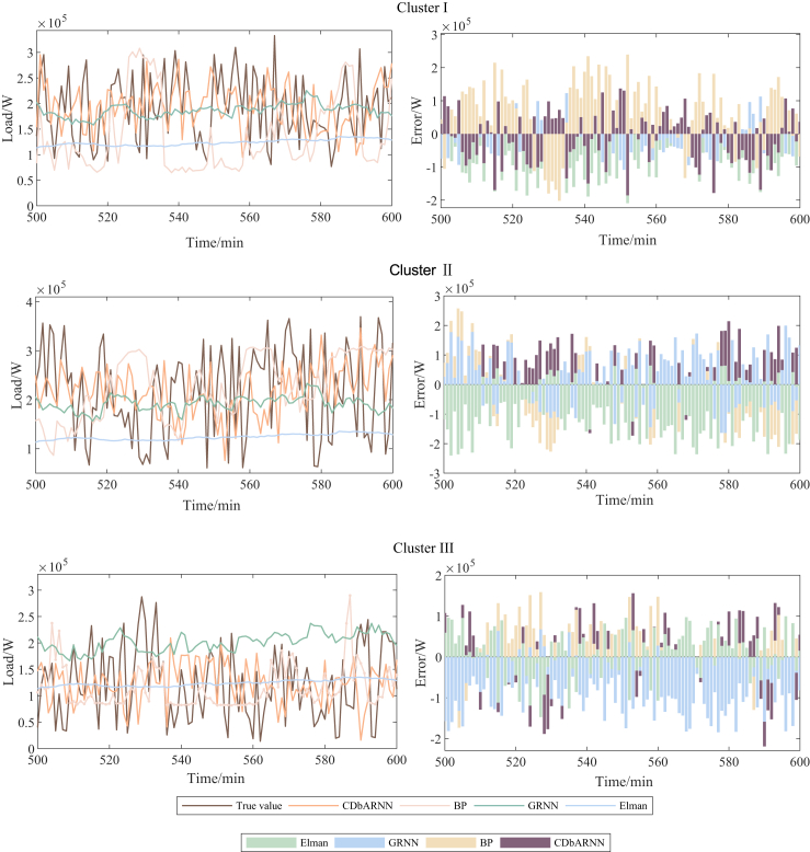
In order to further verify the effectiveness of the CDbARNN, several classic deep learning methods, which include generalized regression neural network (GRNN), back-propagation (BP), and Elman, are employed for comparison. BP is a well-established and widely utilized ANN model known for its ability to learn and store complex mapping relationships. It has been extensively applied in various fields due to its capability to handle non-linear relationships and learn intricate patterns. GRNN, on the other hand, has demonstrated superior approximation capability and faster learning speed compared to other traditional ANN models, especially when the available sample data is limited. This makes GRNN a suitable candidate for STLF that often involve limited historical data. Lastly, the Elman network is chosen because it requires a relatively smaller amount of data samples for effective training. This is particularly advantageous when dealing with situations where the available data are scarce or insufficient. By employing these three models, the authors aimed to assess the performance and validity of CDbARNN against established and widely used ANN models, while also considering the unique strengths and advantages offered by each model.^36,37 Table 3 shows the evaluation indicators of the forecasting results of each model. As can be seen from it, when compared with the other three methods in Scenario 1, the performance of CDbARNN also stands out with at least 4.2%, 5.48%, and 9.58% decreases in NMAE, NRMSE, and MAPE, respectively, and at most 0.29 improvement in IA. Among them, GRNN adopts four cross-validation methods to train the neural network and finds the best SPREAD value by looping, but the effect is still not as good as that of the proposed CDbARNN. Elman and BP use the training set to train the network, which is then used to forecast. The different division of the training and test sets will result in unstable forecasting results and over-fitting. While based on the combination of STI and RC, there is essentially no training process in CDbARNN. The input load series reconstructs an input matrix with the load curves in the cluster after K-means clustering and DR. And once the input matrix is entered into CDbARNN, the next step of load values can be forecasted. As a result, CDbARNN outperforms other models on STLF, no matter in accuracy or application.

Figure 9.

Comparison of CDbARNN and other models for forecasting in the three clusters.

Figure 10.

Comparison of CDbARNN and other models for forecasting in the curves randomly generated.

Table 3.

Performance comparison of CDbARNN with other methods

Evaluation metric	Forecasting method	Scenario 1			Scenario 2
		I	II	III	I	II	III
NMAE (%)	CDbARNN	3.86	3.98	5.33	11.44	16.11	19.01
	GRNN	5.86	9.54	15.56	13.53	16.55	22.29
	Elman	5.36	13.67	12.13	17.17	20.16	21.39
	BP	8.06	8.11	15.58	17.23	20.02	20.89
NRMSE(%)	CDbARNN	5.87	5.83	7.67	14.47	19.83	23.20
	GRNN	7.89	12.05	20.25	16.80	19.99	27.26
	Elman	7.23	18.56	17.56	22.07	25.10	26.17
	BP	11.26	10.54	21.57	22.56	24.55	26.45
MAPE(%)	CDbARNN	11.67	11.71	14.78	54.75	66.98	73.36
	GRNN	15.96	31.96	43.67	57.41	76.70	91.84
	Elman	16.53	29.82	26.96	55.56	73.75	73.97
	BP	21.25	30.21	40.91	56.51	71.32	79.87
IA	CDbARNN	0.98	0.98	0.93	0.69	0.62	0.42
	GRNN	0.94	0.90	0.68	0.62	0.58	0.40
	Elman	0.95	0.75	0.66	0.57	0.51	0.40
	BP	0.90	0.94	0.64	0.58	0.59	0.41

Through the forecasting results and errors in Figures 9 and 10, it can be observed that CDbARNN is closer to the true value in Scenario 1, and in Scenario 2 it can forecast the actual load trend comparing with GRNN, Elman and BP.

Statistical tests

To evaluate the performance of the proposed CDbARNN, we compare it with ARNN, CDbARNNwNNO, GRNN, Elman, and BP models. Each model is run independently for 50 times. To determine the statistical significance of the forecasting errors between CDbARNN and the other five models, we employ the Wilcoxon Signed-Rank $t$-Test, which is a non-parametric hypothesis testing method.³⁸ The Wilcoxon Signed-Rank $t$-Test is used to compare two independent samples of equal sample size. A negative $t$-test value indicates that CDbARNN outperforms the corresponding algorithm in terms of both mean and standard deviation, and vice versa. The $p$-value is calculated, and if it is less than 0.05, it indicates that the difference between the two samples is statistically significant. The comparison results are presented in Table 4. It can be observed that all five $t$-Test values are negative, and the corresponding $p$-values are within acceptable limits. This indicates that CDbARNN performs better than the other five models, and the differences in the forecasting errors are statistically significant.

Table 4.

Statistical tests of ARNN, CDbARNNwNNO, GRNN, Elman, BP and CDbARNN

	ARNN	CDbARNNwNNO	GRNN	Elman	BP
$p$-value	0.0189	0.0480	2.508e-10	2.873e-05	3.153e-43
$t$-Test	−564.016	−393.593	−1973.317	−1457.048	−1896.894

Model

In order to overcome the forecasting difficulties of ARNN when the dimensions of the data are not sufficiently high, this paper proposes CDbARNN, which is driven by K-means clustering and the DR technique, for STLF of industrial park. In this section, the forecasting framework of CDbARNN is formulated. The calculation process of this model is divided into the following four steps, and the logical framework of each step is shown in Figure 11.

Figure 11.

The flow chart of CDbARNN.

Step 1

The load data is organized on a daily basis, where each row corresponds to a different day and each column represents a different time point. To capture the similarity in the daily electricity consumption within the power park, we apply K-means clustering to classify the historical load data samples. This classification groups together days with similar power load trends and amplitudes, which prepares the data for subsequent DR and reorganization of the input matrix.

Step 2

We construct a DR technology for the short-term load series, which refers to the one-dimensional load data that requires forecasting. By setting an appropriate similarity parameter, we compare the input load series with the load clusters generated in Step 1 during the same time period. We consider various factors such as maximum value, slope, power magnitude similarity, and step similarity to determine the cluster to which the series belongs.

Step 3

Based on the results of DR, we reconstruct the short-term high-dimensional input load matrix. To obtain the optimal number of reservoir nodes for subsequent forecasting, we employ the evolutionary predator and prey strategy (EPPS).³⁹ If the input load series belongs to cluster $k$, we combine the series with the load data in cluster $k$ to form the new input matrix and determine the corresponding optimal number of neural network reservoir nodes.

Step 4

The reconstructed matrix is then fed into CDbARNN, with CDbARNNReservoir utilizing the optimal number of nodes corresponding to cluster $k$ obtained in Step 3. By integrating the STI equation and the RC structure, we extract the power consumption regularity of the park and iteratively solve the matrix containing future load information. This iterative approach allows for rolling backward forecasting.

K-means clustering of CDbARNN

In STLF, historical data show a certain correlation, so it is an effective way to improve the forecasting accuracy by investigating the similarity. According to the test samples with better data correlation, more accurate forecasting results can be obtained. Although high-dimensional data contain rich information, they can also introduce noise into the prediction if some of the high-dimensional variables are irrelevant to the target variable. Our primary objective is to select relevant variables or eliminate irrelevant variables from the high-dimensional data, which can significantly improve the performance of ARNN in practical applications. In this study, we chose K-means clustering for load curve clustering. K-means clustering provides comprehensive information and has a clear and simple change rule, making it easy to comprehend.⁴⁰ The principle of K-means clustering is relatively simple, easy to implement, and produces interpretable results.⁴¹ In previous studies, K-means clustering has been used for load decomposition. For example, Chen et al. used K-means clustering for the early classification and cluster labeling.⁴¹ Al-Wakeel et al. proposed a load estimation algorithm based on K-means clustering.⁴²

Algorithm 1. The pseudocode of K-means clustering in CDbARNN

1.Randomly select $k$ points in the data sample as the initial cluster centers of the $k$ clusters.

2.Compute the distance of each data sample to $k$ cluster centers, and divide it into $k$ clusters according to the closest distance.

3.Find the mean vectors for the $k$ clusters and use the $k$ mean vectors as the new cluster centers for each cluster.

4.Repeat 2 to 3 until the cluster center no longer changes.

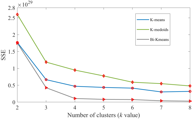
In this study, the 365-day load curves of an industrial park in Zibo city, China, is used as historical dataset. In the K-means clustering algorithm, the determination of $k$ value is a critical step. In this case, we employ the elbow method to calculate the $k$ value of different clustering methods, including K-means, K-medoids, and BiKmeans. The sum of squared errors (SSE) is used to describe the elbow method, which is an effective method to determine the optimal number of clusters based on the change in slope. As the $k$ value increases, the position where the improvement effect of the distortion degree decreases the most is the $k$ value corresponding to the elbow.⁴³ It can be seen from Figure 12 that $k=3$ is the elbow inflection point and the most suitable number of clusters is 3, regardless of the clustering method used, be it K-means, K-medoids, or BiKmeans. Therefore, we selected K-means clustering for this study due to its computational efficiency and effectiveness in yielding results.

Figure 12.

SSE with different $k$ values.

Figure 13 shows the clustering results of the 365-day load curves. Data are collected every minute, and 1440 data points are collected each day. As shown by Figure 13, load curves are divided into three clusters, denoted as I, II and III, and the corresponding cluster centers of these clusters are also provided on the second column of the figure. It can be seen from Figure 13 that the power load during the day time is significantly higher than that at night time because the park starts work at 8:00 a.m. and leaves work at 5:00 p.m. Besides, the load curve has strong volatility. Clusters I and II rise in a straight line, while Cluster III rises in a downward spiral. There is also a difference in the degree of sudden increase and decrease in Clusters I and II. The range of maximum and minimum values varies for each cluster.

Figure 13.

Clustering results of 365-day load curves.

Dynamic recognition of CDbARNN

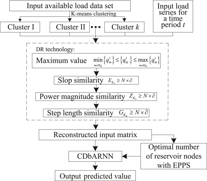
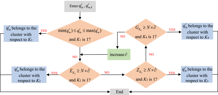
DR is a similar segment search technology that identifies which cluster the load series entered into CDbARNN belongs to. And then a high-dimensional dataset is reconstructed by using all the datasets in this cluster and the input load series. After K-means clustering and DR, it can effectively eliminate the data unrelated to the forecasting target and improve the forecasting accuracy. The detailed steps of DR algorithm are as follows.

Step 1: Comparison of the maximum and minimum of the input load series with the load curves in each cluster.

Compare the magnitude of the input load series $q_{\text{in}}^t={\left\{q_{\text{in}}^{t,1},q_{\text{in}}^{t,2},\dots ,q_{\text{in}}^{t,N}\right\}}_{1\times N}$ with all load curves $q_m^t={\left\{q_m^{t,1},q_m^{t,2},\dots ,q_m^{t,N}\right\}}_{K\times N}$, where $K$ denotes the number of clusters, $N$ is the length of input load series at time $t$. At time $t$, if $q_{\text{in}}^t$ belongs to cluster $k$ of the load, each value of $q_{\text{in}}^t$ must be between the minimum and maximum of the corresponding $q_m^t$.

$$\underset{m\in M_k}{\min }\left\{q_m^{t,n}\right\}\le \left\{q_{\text{in}}^{t,n}\right\}\le \underset{m\in M_k}{\max }\left\{q_m^{t,n}\right\}$$ (Equation 2)

where $n\in \left\{\mathrm{1,2},\dots ,N\right\}$, and $M_k$ is the number of the load curves in cluster $k$.

Assume that $K_1$ is the number of clusters that satisfies Equation (Equation 1a), (Equation 1b), (Equation 1c), (Equation 1d). If $K_1$ is 1, $q_{\text{in}}^t$ belongs to the only cluster. If there is more than one cluster satisfying Equation (Equation 1a), (Equation 1b), (Equation 1c), (Equation 1d), i.e., $K_1>1$, proceed to the next step.

Step 2: Comparison of the slope similarity of the input load series with the load curves in the cluster with respect to $K_1$.

Assume that $q_{k\left(K_1\right)}^t={\left\{q_{k\left(K_1\right)}^{t,1},q_{k\left(K_1\right)}^{t,2},\dots ,q_{k\left(K_1\right)}^{t,N}\right\}}_{K_1\times N}$ is the cluster centers with respect to $K_1$. Calculate the slope of $q_{\text{in}}^t$ in each adjacent time interval and count it as $s_{\text{in}}^t={\left\{s_{\text{in}}^{t,1},s_{\text{in}}^{t,2},\dots ,s_{\text{in}}^{t,N-1}\right\}}_{1\times \left(N-1\right)}$, i.e., $s_{\text{in}}^{t,n}=\left(q_{\text{in}}^{t,n}-q_{\text{in}}^{t,n-1}\right)/\Delta t$, where $\Delta t$ is the time interval between adjacent sampling points. And the slope direction is denoted as $p_{\text{in}}^t={\left\{p_{\text{in}}^{t,1},p_{\text{in}}^{t,2},\dots ,p_{\text{in}}^{t,N-1}\right\}}_{1\times \left(N-1\right)}$. Similarly, calculate the slop of $q_{k\left(K_1\right)}^t$ in each adjacent time interval and count it as $s_{k\left(K_1\right)}^t={\left\{s_{k\left(K_1\right)}^{t,1},s_{k\left(K_1\right)}^{t,2},\dots ,s_{k\left(K_1\right)}^{t,N-1}\right\}}_{K_1\times \left(N-1\right)}$, i.e.,

$s_{k\left(K_1\right)}^{t,n}=\left(q_{k\left(K_1\right)}^{t,n}-q_{k\left(K_1\right)}^{t,n-1}\right)/\Delta t$. And the slope direction can be expressed as $p_{k\left(K_1\right)}^t={\left\{p_{k\left(K_1\right)}^{t,1},p_{k\left(K_1\right)}^{t,2},\dots ,p_{k\left(K_1\right)}^{t,N-1}\right\}}_{K_1\times \left(N-1\right)}$. The counting rules are shown as follows:

$$p_{\text{in}}^{t,n}=\{\begin{array}{c}1,s_{\text{in}}^{t,n}>0\\ 0,s_{\text{in}}^{t,n}=0\\ -1,s_{\text{in}}^{t,n}<0\end{array}$$ (Equation 3)

$$p_{k\left(K_1\right)}^{t,n}=\{\begin{array}{c}1,s_{k\left(K_1\right)}^{t,n}>0\\ 0,s_{k\left(K_1\right)}^{t,n}=0\\ -1,s_{k\left(K_1\right)}^{t,n}<0\end{array}$$ (Equation 4)

If the slope $s_{\text{in}}^{t,n}$ or $s_{k\left(K_1\right)}^{t,n}$ is positive, the corresponding slope direction $p_{\text{in}}^{t,n}$ or $p_{k\left(K_1\right)}^{t,n}$ is 1. If the slope $s_{\text{in}}^{t,n}$ or $s_{k\left(K_1\right)}^{t,n}$ is 0, the corresponding slope direction $p_{\text{in}}^{t,n}$ or $p_{k\left(K_1\right)}^{t,n}$ is 0. If the slope $s_{\text{in}}^{t,n}$ or $s_{k\left(K_1\right)}^{t,n}$ is negative, the corresponding slope direction $p_{\text{in}}^{t,n}$ or $p_{k\left(K_1\right)}^{t,n}$ is $-1$. Then we define the binary variables $e_{k\left(K_1\right)}^t={\left\{e_{k\left(K_1\right)}^{t,1},\dots ,e_{k\left(K_1\right)}^{t,N}\right\}}_{K_1\times N}$ for each cluster associated with $K_1$, where $e_{k\left(K_1\right)}^{t,n}\in \left\{\mathrm{0,1}\right\}$. If $p_{\text{in}}^{t,n}$ equals to $p_{k\left(K_1\right)}^{t,n}$ , $e_{k\left(K_1\right)}^{t,n}$ is counted as 1. Otherwise, it is counted as 0. Summing over $e_{k\left(K_1\right)}^{t,n}$ yields $E_{k\left(K_1\right)}$.

$$e_{k\left(K_1\right)}^{t,n}=\{\begin{array}{c}1,p_{\text{in}}^{t,n}=p_{k\left(K_1\right)}^{t,n}\\ 0,p_{\text{in}}^{t,n}\ne p_{k\left(K_1\right)}^{t,n}\end{array}$$ (Equation 5)

$$E_{k\left(K_1\right)}=\sum _{n=1}^N{e}_{k\left(K_1\right)}^{t,n}$$ (Equation 6)

$E_{k\left(K_1\right)}$ indicates a slope similarity, the larger the value of $E_{k\left(K_1\right)}$, the higher the similarity between $q_{\text{in}}^t$ and $q_{k\left(K_1\right)}^t$. Assume that the similarity rate $\partial$ is 90 $\%$, and $K_2$ is the number of cluster that satisfies $E_{k\left(K_2\right)}\ge N\times \partial$. If $K_2$ is 1, $q_{\text{in}}^t$ belongs to the only cluster. If there is more than one cluster satisfying $E_{k\left(K_2\right)}\ge N\times \partial$, i.e., $K_2>1$, proceed to the next step.

Step 3: Comparison of the power magnitude similarity of the input load series with the load curves in the cluster with respect to $K_2$.

Assume that $q_{k\left(K_2\right)}^t={\left\{q_{k\left(K_2\right)}^{t,1},q_{k\left(K_2\right)}^{t,2},\dots ,q_{k\left(K_2\right)}^{t,N}\right\}}_{K_2\times N}$ is the cluster centers with respect to $K_2$. Calculate the difference between $q_{\text{in}}^t$ and $q_{k\left(K_2\right)}^t$ at each sampling point and count it as $\Delta q_{k\left(K_2\right)}^t=\left|q_{\text{in}}^t-q_{k\left(K_2\right)}^t\right|$. Then we define the binary series $z_{k\left(K_2\right)}^t={\left\{z_{k\left(K_2\right)}^{t,1},\dots ,z_{k\left(K_2\right)}^{t,N}\right\}}_{K_2\times N}$ for the cluster with respect to $K_2$, where $z_{k\left(K_2\right)}^{t,n}\in \left\{\mathrm{0,1}\right\}$. We define $\Delta q_{k\left(K_2^{\prime }\right)}^{t,n}$ as the minimum value of $\Delta q_{k\left(K_2\right)}^{t,n}$. The $z_{k\left(K_2\right)}^{t,n}$ corresponding to the cluster of $\Delta q_{k\left(K_2^{\prime }\right)}^{t,n}$ is counted as 1, and others are counted as 0. Summing over $z_{k\left(K_2\right)}^{t,n}$ yields power magnitude similarity $Z_{k\left(K_2\right)}$.

$$z_{k\left(K_2\right)}^{t,n}=\{\begin{array}{cc}1\text{,}& \text{if}\Delta q_{k\left(K_2\right)}^{t,n}=\min \left(\Delta q_{k\left(K_2\right)}^{t,n}\right)\\ 0\text{,}& \text{otherwise}\end{array}$$ (Equation 7)

$$Z_{k\left(K_2\right)}=\sum _{n=1}^N{z}_{k\left(K_2\right)}^{t,n}$$ (Equation 8)

$Z_{k\left(K_2\right)}$ indicates a power magnitude similarity, the larger the value of $Z_{k\left(K_2\right)}$, the higher the similarity between $q_{\text{in}}^t$ and $q_{k\left(K_2\right)}^t$. Assume that $K_2$ is the number of clusters that satisfies $Z_{K_3}\ge N\times \partial$. If $K_3$ is 1, $q_{\text{in}}^t$ belongs to the only cluster. If there is more than one cluster satisfying the condition, i.e., $K_3>1$, proceed to the next step.

Step 4: Comparison of the step length similarity between the input load series with the load curves in the cluster with respect to $K_3$.

Assume that $q_{k\left(K_3\right)}^t={\left\{q_{k\left(K_3\right)}^{t,1},q_{k\left(K_3\right)}^{t,2},\dots ,q_{k\left(K_3\right)}^{t,N}\right\}}_{K_3\times N}$ is the cluster centers of the clusters with respect to $K_3$. Calculate the straight line distance between two adjacent sampling points in $q_{\text{in}}^t$, and count it as $d_{\text{in}}^t={\left\{d_{\text{in}}^{t,1},d_{\text{in}}^{t,2},\dots ,d_{\text{in}}^{t,N}\right\}}_{1\times N}$. Similarly, calculate the straight line distance between two adjacent sampling points in $q_{k\left(K_3\right)}^t$, and count it as $d_{k\left(K_3\right)}^t={\left\{d_{k\left(K_3\right)}^{t,1},d_{k\left(K_3\right)}^{t,2},\dots ,d_{k\left(K_3\right)}^{t,N}\right\}}_{K_3\times N}$. Then, let $d_{\text{in}}^t$ minus $d_{k\left(K_3\right)}^t$ to get the difference $L_{k\left(K_3\right)}^t$.

$$d_{\text{in}}^{t,n}=\sqrt{\Delta t^2+{\left(q_{\text{in}}^{t,n}-q_{\text{in}}^{t,n-1}\right)}^2}$$ (Equation 9a)

$$d_{k\left(K_3\right)}^{t,n}=\sqrt{\Delta t^2+{\left(q_{k\left(K_3\right)}^{t,n}-q_{k\left(K_3\right)}^{t,n-1}\right)}^2}$$ (Equation 9b)

$$L_{k\left(K_3\right)}^{t,n}=\left|d_{\text{in}}^{t,n}-d_{k\left(K_3\right)}^{t,n}\right|$$ (Equation 10)

Define binary series $g_{k\left(K_3\right)}^t={\left\{g_{k\left(K_3\right)}^{t,1},\dots ,g_{k\left(K_3\right)}^{t,N}\right\}}_{K_3\times N}$ for each cluster with respect to $K_3$, where $g_{k\left(K_3\right)}^{t,n}\in \left\{\mathrm{0,1}\right\}$. The $g_{k\left(K_3\right)}^t$ of the load cluster corresponding to the minimum value of $L_{k\left(K_3\right)}^{t,n}$ is counted as 1, and the rest of the load clusters are counted as 0. Summing over $g_{k\left(K_3\right)}^{t,n}$ yields step length similarity $G_{K_3}$.

$$g_{k\left(K_3\right)}^{t,n}=\{\begin{array}{cc}1\text{,}& \text{if}{L}_{k\left(K_3\right)}^{t,n}=\min \left(L_{k\left(K_3\right)}^{t,n}\right)\\ 0\text{,}& \text{otherwise}\end{array}$$ (Equation 11)

$$G_{K_3}=\sum _{n=1}^N{g}_{k\left(K_3\right)}^{t,n}$$ (Equation 12)

$G_{K_3}$ indicates a step length similarity, the larger the value of $G_{K_3}$, the higher the similarity between $q_{\text{in}}^t$ and $q_{k\left(K_3\right)}^t$. Assume that $K_4$ is the number of clusters that satisfies $G_{K_4}\ge N\times \partial$. If $K_4$ is 1, $q_{\text{in}}^t$ belongs to the only cluster. If there is more than one cluster satisfying the condition, i.e., $K_4>1$, increases the value of $\partial$, and repeat from Step 2 to Step 4 until get out of the loop. Figure 14 shows the overview of the proposed DR technique.

Figure 14.

The flow chart of DR.

When the input load series corresponds to a holiday or experiences sudden changes due to weather, the DR technology employed in this paper can identify whether the curve belongs to the existing clusters. If the load series does not belong to any of the existing clusters, it is treated as a new cluster. However, it should be noted that in such cases, where there are significant changes in load patterns, the accuracy of CDbARNN’s forecasting may be comparable to that of other methods. This is because the model may not be able to capture enough spatial information to accurately predict load variations.

CDbARNN

In contrast to traditional statistics-based machine learning, CDbARNN opens a new way for dynamics-based machine learning based on STI and RC. CDbARNN capitalizes on RC structure and STI transformation, but the two are by no means a simple combination. To be specific, assuming that after clustering and DR, a $N$-dimensional reconstructed load vector matrix $Q^t$ with $N$ columns and $M_k$ rows is entered into CDbARNN. And according to the delay-embedding theory, a one-dimensional vector $R^t={\left(r^t,r^{t+1},\dots ,r^{t+D}\right)}^{\mathrm{T}}$ which contains the forecasting value we expect to obtain can be maped from $Q^t$. $D$ is the forecasting step size. CDbARNN can be represented by the following equations:

$$\{\begin{array}{c}UF\left(Q^t\right)=R^t\\ F\left(Q^t\right)=V{R}^t\end{array}$$ (Equation 13)

where $UV=I$, $U$ is a $D\times N$ matrix, and $V$ is a $N\times D$ matrix. They are unknown parameters in advance. $I$ is a $D\times D$ identity matrix. The multi-layer feedforward neural network $F$ whose weights are randomly given beforehand and fixed has four layers. By iteratively using the ordinary least square method to solve $U$, $V$ and $R^t$, the forecasting values involved in $R^t$ can be generated.

As shown in Figure 15, the yellow dashed box is the reservoir of CDbARNN, with four layers and different numbers of nodes, but the weights between neurons are not involved in the training. In traditional RC, the middle layer’s reservoir matrix is randomly generated and remains unchanged.⁴⁴ However, by combining RC and STI, CDbARNN converts $Q_t$ into cluster and DR based reservoir (CDbReservoir) and obtains a high-dimensional spatial information $F\left(Q^t\right)$. Then $R_t$ involved target load forecasting value is maped from $F\left(Q^t\right)$. Furthermore, this framework’s CDbReservoir matches the optimal node numbers for different clusters of loads.

Unlike traditional RC models that rely on external/additional dynamics irrelevant to the target system, CDbARNN transforms the dynamics of the observed high-dimensional data as the reservoir, thereby exploiting the intrinsic dynamics of the observed/target system. By using a nonlinear function F as the reservoir structure based on both the primary and conjugate forms of the STI equations, we construct the CDbARNN-based equations. This enables CDbARNN to encode $F\left(Q^t\right)$ to $R^t$ and decode $R^t$ to $F\left(Q^t\right)$, where the $R^t$ is the temporal (one-dimensional) dynamics across multiple time points and $Q_t$ is the spatial (high-dimensional) information at one time point. CDbARNN has been successfully applied to both representative models and real-world datasets, demonstrating satisfactory performance in multi-step-ahead prediction, even in the presence of noise and time-varying systems. The CDbARNN transformation effectively expands the sample size and holds great potential for practical applications in artificial intelligence and machine learning.

Discussion

This study introduces a novel STLF method called clustering and DR–based auto-reservoir neural network (CDbARNN). The historical available load data samples from an industrial park microgrid in Zibo city, China, spanning 365 days and from 0:00 to 23:00, are analyzed to identify electricity consumption patterns. Utilizing K-means clustering, the load data is categorized into three clusters based on daily characteristics. Scenarios 1 and 2 are employed to assess the accuracy and versatility of CDbARNN. The results demonstrate that CDbARNN outperforms other methods in STLF. Its precise forecasting enables better power dispatching and improved utilization of electricity resources, leading to reduced waste. The key conclusions of this study are summarized as follows.

• (1)By leveraging K-means clustering and DR, CDbARNN achieves higher accuracy compared to ARNN. In the performance comparison of CDbARNN with ARNN and CDbARNNwNNO, the maximum reductions in NMAE, NRMSE, and MAPE are 3.28%, 4.25%, and 10.25%, respectively. Additionally, the maximum improvement in IA is 0.06.
• (2)CDbARNN, with input load series lengths of 30 steps, 20 steps, and 10 steps, exhibits superior forecasting accuracy and robustness compared to both ARNN and CDbARNNwNNO. The comparison of metrics reveals that CDbARNN achieves maximum reductions in NMAE, NRMSE, and MAPE of 0.69%, 1.03%, and 5.26%, respectively, while also demonstrating a maximum improvement of 0.04 in IA. Furthermore, when comparing different input lengths of CDbARNN, the maximum reductions in NMAE, NRMSE, MAPE, and IA are 0.67%, 0.89%, 7.92%, and 0.04, respectively.
• (3)CDbARNN not only captures the nonlinear mapping relationship of the load but also effectively extracts and utilizes the temporal characteristics of the time series. When compared to Elman, GRNN, and BP, CDbARNN achieves maximum reductions in NMAE, NRMSE, and MAPE of 10.25%, 13.9%, and 28.89%, respectively. Furthermore, the maximum improvement in IA is 0.29. Therefore, CDbARNN successfully learns the distinctive characteristics of similar load curves and reconstructs the input matrix, resulting in more accurate forecasting outcomes with limited load data.

Limitations of the study

The main limitation of the proposed model lies in the lack of comprehensive analysis regarding the influence of uncertainty coupling between power load and renewable energy on the clustering and DR. Additionally, we have not taken into account the coupling relationship between active and reactive power in reality, such as voltage offset and power factor range, which directly impact active and reactive power. In our future work, we plan to investigate STLF considering these coupling characteristics.

STAR★Methods

Key resources table

REAGENT or RESOURCE	SOURCE	IDENTIFIER
Software and algorithms
Basic Model	GitHUb	https://github.com/RPcb/ARNN
Comparison Model	Electrical load forecasting: modeling and model construction	N/A

Resource availability

Lead contact

Further information and requests for resources should be directed to and will be fulfilled by the lead contact, Jiajia Chen (jjchen@sdut.edu.cn).

Materials availability

This study did not generate new unique reagents.

Published: July 22, 2023

Data and code availability

• $•$ Data: The data that support the findings of this study are available on request from the corresponding author Jiajia Chen (jjchen@sdut.edu.cn) upon reasonable request.

• $•$ Code: The code that support the findings of this study are available on request from the corresponding author Jiajia Chen (jjchen@sdut.edu.cn) upon reasonable request.

References

- 1.Liang Y., Niu D., Hong W.-C. Short term load forecasting based on feature extraction and improved general regression neural network model. Energy. 2019;166:653–663. doi: 10.1016/j.energy.2018.10.119. [DOI] [Google Scholar]
- 2.Chu Y., Li M., Coimbra C.F.M., Feng D., Wang H. Intra-hour irradiance forecasting techniques for solar power integration: a review. iScience. 2021;24 doi: 10.1016/j.isci.2021.103136. [DOI] [PMC free article] [PubMed] [Google Scholar]
- 3.Yang D., Guo J.-E., Sun S., Han J., Wang S. An interval decomposition-ensemble approach with data-characteristic-driven reconstruction for short-term load forecasting. Appl. Energy. 2022;306 doi: 10.1016/j.apenergy.2021.117992. [DOI] [Google Scholar]
- 4.Willems N., Sekar A., Sigrin B., Rai V. Forecasting distributed energy resources adoption for power systems. iScience. 2022;25 doi: 10.1016/j.isci.2022.104381. [DOI] [PMC free article] [PubMed] [Google Scholar]
- 5.Jenn A., Highleyman J. Distribution grid impacts of electric vehicles: A California case study. iScience. 2022;25 doi: 10.1016/j.isci.2021.103686. [DOI] [PMC free article] [PubMed] [Google Scholar]
- 6.Kittel M., Schill W.P. Renewable energy targets and unintended storage cycling: Implications for energy modeling. iScience. 2022;25 doi: 10.1016/j.isci.2022.104002. [DOI] [PMC free article] [PubMed] [Google Scholar]
- 7.Lin J., Abhyankar N., He G., Liu X., Yin S. Large balancing areas and dispersed renewable investment enhance grid flexibility in a renewable-dominant power system in China. iScience. 2022;25 doi: 10.1016/j.isci.2022.103749. [DOI] [PMC free article] [PubMed] [Google Scholar]
- 8.Sharma S., Majumdar A., Elvira V., Chouzenoux E. Blind Kalman Filtering for Short-Term Load Forecasting. IEEE Trans. Power Syst. 2020;35:4916–4919. [Google Scholar]
- 9.Singh K.K., Kumar S., Dixit P., Bajpai M.K. Kalman filter based short term prediction model for COVID-19 spread. Appl. Intell. 2021;51:2714–2726. doi: 10.1007/s10489-020-01948-1. [DOI] [PMC free article] [PubMed] [Google Scholar]
- 10.Amjady N. Short-Term Hourly Load Forecasting Using Time-Series Modeling With Peak Load Estimation Capability. IEEE Trans. Power Syst. 2001;16:498–505. doi: 10.1109/59.932287. [DOI] [Google Scholar]
- 11.Sadaei H.J., Guimarães F.G., José da Silva C., Lee M.H., Eslami T. Short-term load forecasting method based on fuzzy time series, seasonality and long memory process. Int. J. Approx. Reason. 2017;83:196–217. doi: 10.1016/j.ijar.2017.01.006. [DOI] [Google Scholar]
- 12.Oreshkin B.N., Dudek G., Pełka P., Turkina E. N-BEATS neural network for mid-term electricity load forecasting. Appl. Energy. 2021;293 doi: 10.1016/j.apenergy.2021.116918. [DOI] [Google Scholar]
- 13.Vrablecová P., Bou Ezzeddine A., Rozinajová V., Šárik S., Sangaiah A.K. Smart grid load forecasting using online support vector regression. Comput. Electr. Eng. 2018;65:102–117. doi: 10.1016/j.compeleceng.2017.07.006. [DOI] [Google Scholar]
- 14.Baesmat K.H., Masodipour I., Samet H. Improving the Performance of Short-Term Load Forecast Using a Hybrid Artificial Neural Network and Artificial Bee Colony Algorithm Amélioration des performances de la prévision de la charge à court terme à l’aide d’un réseau neuronal artificiel hybride et d’un algorithme de colonies d’abeilles artificielles. IEEE Can. J. Electr. Comput. Eng. 2021;44:275–282. doi: 10.1109/icjece.2021.3056125. [DOI] [Google Scholar]
- 15.Yang Y., Yu Y., Yang N.N., Huang B., Kuang Y.F., Liao Y.W. Sequential grid approach based support vector regression for short-term electric load forecasting. Appl. Energy. 2019;80:1010–1021. doi: 10.1016/j.apenergy.2019.01.127. [DOI] [Google Scholar]
- 16.Lu J., Wang Z., Cao J., Ho D.W., Kurths J. Pinning Impulsive Stabilization of Nonlinear Dynamical Networks with Time-Varying Delay. Int. J. Bifurcation Chaos. 2012;22:1250176. doi: 10.1142/s0218127412501763. [DOI] [Google Scholar]
- 17.Hafeez G., Khan I., Jan S., Shah I.A., Khan F.A., Derhab A. A novel hybrid load forecasting framework with intelligent feature engineering and optimization algorithm in smart grid. Appl. Energy. 2021;299 doi: 10.1016/j.apenergy.2021.117178. [DOI] [Google Scholar]
- 18.Jiang L., Wang X., Li W., Wang L., Yin X., Jia L. Hybrid Multitask Multi-Information Fusion Deep Learning for Household Short-Term Load Forecasting. IEEE Trans. Smart Grid. 2021;12:5362–5372. doi: 10.1109/tsg.2021.3091469. [DOI] [Google Scholar]
- 19.Crone S.F., Hibon M., Nikolopoulos K. Advances in forecasting with neural networks? Empirical evidence from the NN3 competition on time series prediction. Int. J. Forecast. 2011;27:635–660. doi: 10.1016/j.ijforecast.2011.04.001. [DOI] [Google Scholar]
- 20.Chen P., Liu R., Aihara K., Chen L. Autoreservoir computing for multistep ahead prediction based on the spatiotemporal information transformation. Nat. Commun. 2020;11:4568. doi: 10.1038/s41467-020-18381-0. [DOI] [PMC free article] [PubMed] [Google Scholar]
- 21.Song L., Ding L., Wen T., Yin M., Zeng Z. Time series change detection using reservoir computing networks for remote sensing data. Int. J. Intell. Syst. 2022;37:10845–10860. doi: 10.1002/int.22984. [DOI] [Google Scholar]
- 22.Hart A., Hook J., Dawes J. Embedding and approximation theorems for echo state networks. Neural Network. 2020;128:234–247. doi: 10.1016/j.neunet.2020.05.013. [DOI] [PubMed] [Google Scholar]
- 23.Jaeger H., Lukosevicius M., Popovici D., Siewert U. Optimization and applications of echo state networks with leaky-integrator neurons. Neural Network. 2007;20:335–352. doi: 10.1016/j.neunet.2007.04.016. [DOI] [PubMed] [Google Scholar]
- 24.Li M., Ma S., Liu Z. A novel method to detect the early warning signal of COVID-19 transmission. BMC Infect. Dis. 2022;22:626. doi: 10.1186/s12879-022-07603-z. [DOI] [PMC free article] [PubMed] [Google Scholar]
- 25.Tang Y., Hoffmann A. Quantifying information of intracellular signaling: progress with machine learning. Rep. Prog. Phys. 2022;85:086602. doi: 10.1088/1361-6633/ac7a4a. [DOI] [PMC free article] [PubMed] [Google Scholar]
- 26.Liu R., Zhong J., Hong R., Chen E., Aihara K., Chen P., Chen L. Predicting local COVID-19 outbreaks and infectious disease epidemics based on landscape network entropy. Sci. Bull. 2021;66:2265–2270. doi: 10.1016/j.scib.2021.03.022. [DOI] [PubMed] [Google Scholar]
- 27.Gao R., Du L., Suganthan P.N., Zhou Q., Yuen K.F. Random vector functional link neural network based ensemble deep learning for short-term load forecasting. Expert Syst. Appl. 2022;206 doi: 10.1016/j.eswa.2022.117784. [DOI] [Google Scholar]
- 28.Wang Y., Chen J., Chen X., Zeng X., Kong Y., Sun S., Guo Y., Liu Y. Short-Term Load Forecasting for Industrial Customers Based on TCN-LightGBM. IEEE Trans. Power Syst. 2021;36:1984–1997. doi: 10.1109/tpwrs.2020.3028133. [DOI] [Google Scholar]
- 29.Laouafi A., Laouafi F., Boukelia T.E. An adaptive hybrid ensemble with pattern similarity analysis and error correction for short-term load forecasting. Appl. Energy. 2022;322 doi: 10.1016/j.apenergy.2022.119525. [DOI] [Google Scholar]
- 30.Shaffer B., Quintero D., Rhodes J. Changing sensitivity to cold weather in Texas power demand. iScience. 2022;25 doi: 10.1016/j.isci.2022.104173. [DOI] [PMC free article] [PubMed] [Google Scholar]
- 31.Dai Y., Zhao P. A hybrid load forecasting model based on support vector machine with intelligent methods for feature selection and parameter optimization. Appl. Energy. 2020;279 doi: 10.1016/j.apenergy.2020.115332. [DOI] [Google Scholar]
- 32.Niu D., Wang K., Sun L., Wu J., Xu X. Short-term photovoltaic power generation forecasting based on random forest feature selection and CEEMD: A case study. Appl. Soft Comput. 2020;93 doi: 10.1016/j.asoc.2020.106389. [DOI] [Google Scholar]
- 33.Xie Y., Li C., Li M., Liu F., Taukenova M. An overview of deterministic and probabilistic forecasting methods of wind energy. iScience. 2023;26:105804. doi: 10.1016/j.isci.2022.105804. [DOI] [PMC free article] [PubMed] [Google Scholar]
- 34.Lusis P., Khalilpour K.R., Andrew L., Liebman A. Short-term residential load forecasting: Impact of calendar effects and forecast granularity. Appl. Energy. 2017;205:654–669. doi: 10.1016/j.apenergy.2017.07.114. [DOI] [Google Scholar]
- 35.Shi H., Xu M., Li R. Deep Learning for Household Load Forecasting—A Novel Pooling Deep RNN. IEEE Trans. Smart Grid. 2018;9:5271–5280. doi: 10.1109/tsg.2017.2686012. [DOI] [Google Scholar]
- 36.Gao T., Lu W. Machine learning toward advanced energy storage devices and systems. iScience. 2021;24 doi: 10.1016/j.isci.2020.101936. [DOI] [PMC free article] [PubMed] [Google Scholar]
- 37.Shu X., Shen S., Shen J., Zhang Y., Li G., Chen Z., Liu Y. State of health prediction of lithium-ion batteries based on machine learning: Advances and perspectives. iScience. 2021;24 doi: 10.1016/j.isci.2021.103265. [DOI] [PMC free article] [PubMed] [Google Scholar]
- 38.Conover W.J. john wiley & sons; 1999. Practical Nonparametric Statistics. [Google Scholar]
- 39.Chen J.J., Wu Q.H., Ji T.Y., Wu P.Z., Li M.S. Evolutionary predator and prey strategy for global optimization. Inf. Sci. 2016;327:217–232. doi: 10.1016/j.ins.2015.08.014. [DOI] [Google Scholar]
- 40.Ikotun A.M., Ezugwu A.E., Abualigah L., Abuhaija B., Heming J. K-means clustering algorithms: A comprehensive review, variants analysis, and advances in the era of big data. Inf. Sci. 2023;622:178–210. doi: 10.1016/j.ins.2022.11.139. [DOI] [Google Scholar]
- 41.Chen Z., Chen Y., Xiao T., Wang H., Hou P. A novel short-term load forecasting framework based on time-series clustering and early classification algorithm. Energy Build. 2021;251 doi: 10.1016/j.enbuild.2021.111375. [DOI] [Google Scholar]
- 42.Al-Wakeel A., Wu J., Jenkins N. k -means based load estimation of domestic smart meter measurements. Appl. Energy. 2017;194:333–342. doi: 10.1016/j.apenergy.2016.06.046. [DOI] [Google Scholar]
- 43.Liu F., Deng Y. Determine the Number of Unknown Targets in Open World Based on Elbow Method. IEEE Trans. Fuzzy Syst. 2021;29:986–995. doi: 10.1109/tfuzz.2020.2966182. [DOI] [Google Scholar]
- 44.Aceituno P.V., Yan G., Liu Y.Y. Tailoring Echo State Networks for Optimal Learning. iScience. 2020;23 doi: 10.1016/j.isci.2020.101440. [DOI] [PMC free article] [PubMed] [Google Scholar]
Associated Data
This section collects any data citations, data availability statements, or supplementary materials included in this article.
Data Availability Statement