

Abstract
The evolution of reduced-order vocal fold models into clinically useful tools for subject-specific diagnosis and treatment hinges upon successfully and accurately representing an individual patient in the modeling framework. This, in turn, requires inference of model parameters from clinical measurements in order to tune a model to the given individual. Bayesian analysis is a powerful tool for estimating model parameter probabilities based upon a set of observed data. In this work, a Bayesian particle filter sampling technique capable of estimating time-varying model parameters, as occur in complex vocal gestures, is introduced. The technique is compared with time-invariant Bayesian estimation and least squares methods for determining both stationary and non-stationary parameters. The current technique accurately estimates the time-varying unknown model parameter and maintains tight credibility bounds. The credibility bounds are particularly relevant from a clinical perspective, as they provide insight into the confidence a clinician should have in the model predictions.
I. INTRODUCTION
Human speech production is a complex nonlinear process comprising coupled interactions between the airflow emanating from the lungs, tissue motion, and concomitant sound generation at the vocal folds, and acoustic resonances of the vocal tract and subglottal system.1 Owing to this complexity, researchers studying the mechanics of human phonation often rely on simplified models designed to capture the predominant physics while eschewing higher order mechanics. Developed models have varying levels of sophistication, ranging from lumped element tissue models with one-dimensional flow and plane wave acoustic solvers2–5 to high fidelity finite element and computational fluid dynamics models;6–11 see Mittal et al.12 and Erath et al.13 for recent reviews of the fluid mechanics of phonation and reduced-order vocal fold modeling, respectively.
Simplified models of human phonation have proven extremely valuable in elucidating the fundamental mechanics of speech. For example, reduced-order models have successfully predicted and reproduced the self-oscillating behavior of the vocal folds,2 the modal response of the vibrating vocal folds,14 illuminated the importance of nonlinear fluid-tissue-acoustic coupling in speech,15,16 and captured the propagation and transmission of acoustic waves within the vocal tract, subglottal system, and biological tissues.3,17 Recently developed models are capable of generating an acoustical output similar to that of a human speaker, with reasonable agreement with relevant clinical measurements, including fundamental frequency, sound pressure level, and flow rate.13,18,19
Beyond the ability to mimic physiological and pathological vocal fold kinematics and acoustical output, considerable research has focused on developing models into diagnostic and treatment tools.20,21 Numerical models can provide an array of synchronous signals and data that are difficult or currently impossible to measure clinically, including contact forces between colliding vocal folds.22 Lumped element models can also be used to explore compensatory behaviors for vocal hyperfunction and how these influence other speech measures. For example, Zañartu et al.23 used a modified body-cover model to explore the influence of posterior glottal opening (PGO) size on acoustic output and the ramifications of increasing lung pressure to compensate for reduced sound pressure level due to the gap.
Simplified vocal fold models have long held the promise of eventually becoming useful diagnostic and treatment tools, though the reality is that few efforts have successfully bridged the gap between modeling and clinical utility. This is due, in part, to structural properties of the model being based upon average measured or observed values from in vivo and ex vivo experiments.2,4,5,13 Recently, considerable efforts have focused on transitioning from generic vocal fold models to more clinically useful patient-specific representations by estimating model parameters from clinical data of individual subjects.24–30 Early efforts extracted vocal fold medial surface kinematics from high speed video at one location, and then inference techniques were employed to estimate reduced-order model parameter values by minimizing the least square residual between specifically chosen Fourier coefficients of the measured waveform and the Fourier coefficients of the waveform produced by the model. The Fourier coefficients which were chosen represented a smooth version of the waveform.24 Further refinements have used multiple points on the glottis27,31 and the full glottal area waveform for matching,32,33 and extended from two- to three-dimensional (3D) models.30,34 Patient-specific models determined from non-linear least squares-based analysis have been used, for example, to classify pathologies25 and vibratory modes in the vocal folds,26 while synthetic vocal fold models have been employed to demonstrate that frequency dependent viscoelastic properties can be extracted using these methods.29
While making great strides toward developing clinically useful models, the least squares-based framework is inherently limited in that it cannot account for measurement uncertainty in the clinical data, incorporating multiple clinical measurements into the estimation is cumbersome, and there is no mechanism to quantify uncertainty associated with the predicted model parameters and the overall model outputs. That is, optimization-based techniques produce a single estimate with no weight given to any other possible combinations of the parameters that also explain the observed data. This can be limiting in the case of vocal fold modeling, as different combinations of the physiological parameters, such as subglottal pressure and a PGO,23 could explain the measured data equally well in the presence of measurement noise. By simply searching for a fit with minimal residual between the nonlinear vocal fold model and the noisy clinical data, it is not always possible to assess the level of information available in the data. As a result, it is not necessarily straightforward for a clinician to assess the degree of confidence they should have in the model predictions when making diagnosis and treatment decisions based upon model outputs.
Bayesian estimation,35 in contrast, is a stochastic framework that enables estimation of parameters and their associated uncertainties. These estimates and uncertainties provide users with a probability which is easily understood and applicable to clinical decision making. Cataldo et al.36 laid the groundwork for incorporating Bayesian analysis into vocal fold parameter estimation. Their work used sampling methods to estimate stationary (time-invariant) parameters of a vocal fold model and demonstrated the capabilities of Bayesian inference to estimate both the model parameters and their uncertainties. Herein, we extend the work of Cataldo et al. by introducing a non-stationary Bayesian inference framework capable of estimating time-varying vocal fold model parameters. Often the changes in structural vocal fold parameters, such as muscle activation or subglottal pressure, during running speech or certain vocal gestures, are indicative of pathologies.37–40 The stationary techniques currently used to infer physiological parameters in vocal fold models inevitably lose and ignore information present in such time-varying measurements. Consequently, the resulting parameter estimates and uncertainties are often poor and misleading.
Herein, a particle filter technique is introduced to facilitate estimation of time-varying parameters. By considering the estimation problem in a non-stationary setting we are able to incorporate knowledge of the uncertainties present within the vocal fold dynamics in a robust manner. We demonstrate that by using non-stationary techniques, estimates can be improved and uncertainty reduced, even when estimating time-invariant parameters, though this is at the cost of increased computational effort. The capabilities of the non-stationary stochastic framework are demonstrated by employing the particle filter estimation scheme to recover model parameters of a low-order vocal fold model representation when simulated measurements (inputs to the particle filter) are corrupted with Gaussian noise. We further investigate the propagation of uncertainty in the measured (input) data into the parameter estimation and associated credibility intervals.
The paper is organized as follows: the stationary Bayesian estimation scheme is reviewed briefly and the non-stationary framework with the associated particle filter technique is developed in Sec. II; the vocal fold model employed in this study is presented in Sec. III; the capabilities and limitations of the time-variant and invariant schemes applied to vocal fold modeling are demonstrated in Sec. IV; and Sec. V provides conclusions and future directions.
II. BAYESIAN ESTIMATION APPLIED TO VOICED SPEECH
The main shortcoming of the traditional least squares framework is that it treats the inference problem as a quest for the single “true” value without consideration of parameter uncertainty. For instance, optimization techniques can compare one candidate solution to another and determine which is more appropriate in terms of the size of a predefined functional, such as a sum-of-squares residual. However, problems arise when the sum-of-squares residual is small; many researchers erroneously equate this scenario to having identified the “exact” solution, while, for ill-posed inverse problems, there may be a large set of candidate solutions that could explain the data within measurement uncertainty. This is especially the case for models involving multiple degrees of freedom.35
In contrast, the Bayesian framework treats all parameters and measurements as random variables and considers the propagation of uncertainty through the measurement equations. Furthermore, while naive least-squares regression focuses on information provided from a set of measurements, Bayesian inference facilitates the inclusion of other information sources into the inference procedure, which can further narrow the probability densities of the inferred parameters. From a clinical standpoint, incorporating the uncertainty present in clinical measurements into patient-specific model development and propagating that uncertainty into the estimated model parameters provides clinicians with quantifiable information about the reliability of the model being developed.
It can be argued that measurement uncertainty could be roughly obtained using sensitivity analysis. However, such an approach is tantamount to simply mapping the posterior probability distribution, whereas additional insights on the measurement uncertainty could be obtained using the Bayesian approach outlined herein. Furthermore, by considering the problem in a Bayesian framework a range of new techniques, such as the particle filter presented in this paper, are available.
To date, Bayesian estimation applied to speech modeling has assumed that model parameters are stationary,28 even though these parameters are typically non-stationary. In Secs. II A and II B, the notation and language of the Bayesian framework for estimating stationary and non-stationary parameters are introduced. Since this work compares a non-stationary estimation technique with current stationary estimation methods, we include a description of the previously demonstrated stationary estimation scheme, along with the new non-stationary method. The two schemes are then employed to infer parameters of a body-cover vocal fold model5 in Sec. IV.
A. General overview
The foundation of Bayesian inference is Bayes' theorem41
| (1) |
where is the posterior probability density function, which contains all probabilistic information about the parameters of interest θ given the observed measurements y. In the case of lumped element speech modeling, θ is the set of reduced-order model parameters of interest that are to be determined from the clinical measurements y. The density is the “prior” probability density, is the “likelihood,” and is the “evidence.” The prior contains known or expected statistical properties of the estimation parameters based on all knowledge available prior to obtaining the measurements. For instance, if subglottal pressure is a model parameter to be inferred, it is known ahead of time that the value cannot be negative, and is likely within a specified bound. The likelihood quantifies the probability of an observed measurement occurring given fixed parameter values; that is, given a particular model with set parameters, what is the likelihood that the measured data would be observed. Lastly, the evidence is given as
| (2) |
which is a normalization constant that ensures that the posterior density satisfies the Law of Total Probability.
In practice, computation of the full posterior is often arduous, particularly for non-linear models;35 as a result, posterior densities may be approximated with point and spread estimates by assuming that the distribution is Gaussian. Two common point estimates are the maximum likelihood estimate (MLE) and the maximum a posteriori (MAP) estimate. The MLE is the parameter set which maximizes the likelihood density and is the set of parameter values that result in the model most closely matching the data. These parameter values typically correspond to the solution obtained by a weighted least-squares regression.35 In contrast, the MAP maximizes the posterior density and represents the most probable parameter set when the measurements are considered in conjunction with any prior information available about the model parameters. The MAP and MLE estimates coincide when no a priori information is available,35 which is termed an “uninformed” prior [i.e., ], as there is no particular θ which is preferred by the prior density.
One additional benefit of the Bayesian framework is the ability to quantify the uncertainty present in an estimate. A typical spread estimate is defined by a credibility set, which is reminiscent of confidence intervals from standard experimental uncertainty.42 Herein, we use so-called marginal credibility intervals to quantify uncertainty in the estimates. These intervals are found by considering the marginal posterior probability densities, the density found when the other parameters are integrated out of the joint posterior density, and computing the end points so that the true value falls within the interval with 95% probability. This procedure requires integration over multiple parameters, which becomes increasingly computationally inefficient as the number of parameters increases. To overcome this problem, sample-based methods can be employed. Various random sampling techniques have been developed, of which Markov chain Monte Carlo is the most well-known.41 All sampling methods involve the evaluation of the densities in Eq. (1) for a range of randomly selected parameter sets; the various techniques have unique ways of identifying the random parameter sets that approximate the posterior distribution. Sample-based methods are versatile, as they easily handle non-linear models and non-standard probability distributions; however, they typically require a large number of samples in order to compute meaningful estimates.35
B. Stationary estimation
To the best of our knowledge, the only instance to date of Bayesian estimation applied to voiced speech is by Cataldo et al.,28,36 wherein they employ a sample-based method, called importance sampling, to estimate stationary vocal fold model parameters. The fundamental premise of importance sampling is that certain values of the inputs are more important to the parameter being estimated than others. As such, a greater weight is allocated to those regions in the parameter space that have a better fit to the measurements. In particular, this involves taking random samples of θ drawn from some proposal distribution and evaluating how well each of the random draws fits the likelihood distribution. This evaluation of the random draw is then used to allocate a weight to that sample; a new ensemble is then constructed by sampling from the random draws in proportion to their computed weight. If the proposal distribution is chosen to be the prior density, then the importance sampling algorithm will approximate the posterior density.43
The importance sampling algorithm requires knowledge of the likelihood density, which can be difficult to derive for highly non-linear models. Furthermore, with the inclusion of measurement noise and uncertainty in other model parameters, the true likelihood density can prove impossible or impractical to compute. In speech modeling, uncertainty in physiological parameters and clinical measures, coupled with a highly non-linear model, renders direct computation of the weights infeasible. To overcome this, Cataldo et al.28,36 proposed the use of a sample based approximation of the likelihood density. Specifically, for three parameter values relating to the vocal fold model they generated a random ensemble. Using each of the sampled parameter sets and a fixed value of the parameter of interest, an ensemble of fundamental frequencies were computed by evaluating the vocal fold model. The likelihood density was then approximated from the samples of the fundamental frequency using kernel density estimation.44 By changing the fixed value of the parameter of interest, they were then able to approximate the likelihood density and subsequently use the importance sampling algorithm to estimate the posterior density.
C. Non-stationary estimation
In the general case of vocal fold modeling, particularly during vocal gestures and running speech, model parameters (e.g., muscle activation, subglottal pressure, etc.) are not constant in time. Rather, these parameters are continuously varying, and are not well captured by stationary parameter estimation procedures. The risk of misdiagnoses is likely to increase when the dynamics of these parameters is not accurately inferred. When stationary estimation techniques are used for non-stationary problems, information is inevitably lost and the resultant estimates and their associated uncertainties are often misleading.35,45
Vocal fold models regularly consist of a series of coupled unsteady differential equations that are approximated via finite difference in time,2,4,18 which can be represented with a discrete state-space model
| (3) |
| (4) |
where the subscript denotes evaluation at time tk, is the state of the system at time tk, is a vector of the state noise, and f is a function describing the evolution of the vocal fold model. Similarly, , and g represent the measurements, observation noise, and the measurement model of the observations, respectively. By representing the problem in a discrete form, sample-based methods can be applied to estimate parameter values and the corresponding uncertainties.35,41,46
The inclusion of observation noise is natural since all practical measurements are corrupted by some form of measurement error. The state noise , alternatively referred to as process noise, models the disconnect between the true physical dynamics and those modeled by the evolution model f. Neglecting state noise implies that there is a greater level of certainty about how the state evolves, which can reduce the influence of the measurements and cause estimates to be misleading in cases where such certainty in the state evolution is not justified. Lumped-element vocal fold models represent a complex physiological system using relatively simple components (masses, springs, and dampers), and as such incorporating state noise is important, as it enhances the predictive power of the non-stationary Bayesian framework.
There are multiple techniques in the Bayesian framework which consider the state and observations together and enable a thorough analysis of their evolution.46 These techniques usually model both the state and observations as stochastic processes. Moreover, it is common to treat the state as a Markov process, such that
| (5) |
and the measurements as a Markov process with respect to the history of , such that
| (6) |
Combining the above Markov properties with the state-space model from Eqs. (3) and (4) yields a so-called Hidden Markov Model.46
Traditionally, stochastic filters such as a particle or Kalman filter are used to model or predict the evolution of the system state from the observations when the system parameters θk are known. Herein, we employ a particle filter to exploit the information present within the Hidden Markov Model and consequently infer the non-stationary vocal fold model parameters θk and their distributions. Particle filters are a sequential Monte Carlo method in which a set of point masses (or “particles”) are used to approximate the sequence of posterior densities.46 In the present work, we are interested in inferring the distribution of the parameters; to achieve this, the time-varying parameters in θk are treated as additional elements of the state . By extending the state space in this manner, the particle filter estimates the densities relating to θk simultaneously with those densities relating to the state . Hence, using a particle filter to explore and infer the extended state space admits an estimate of the parameter distributions.
The goal of a particle filter is to sequentially produce an ensemble of samples for each time tk, referred to as particles which are distributed according to the posterior density for the kth time step, , where . Loosely, each particle can be considered to be an independent model simulation, with the parameters of each model differing between particles. The most common way to ensure these particles are distributed according to the correct distribution is through repeated application of Bayes' theorem and Monte Carlo integration,35,46 accomplished via the sequential importance resampling47 algorithm:
-
(1)
Initialization: Set k = 0 and draw a random ensemble from the prior distribution .
-
(2)
-
(a)
Prediction: For each of the N particles at time tk, draw one new particle from by evaluating Eq. (3) and is defined by the distribution of the state noise.
-
(b)Update: When the measurement at is computed, calculate the relative likelihoods for the new particles
(7) where(8) and is defined by the distribution of the observation noise.
-
(c)
Resample: Generate another ensemble by sampling each with probability .
-
(a)
-
(3)
Loop: If k = K then end, otherwise increase and repeat from step (2).
At first, the algorithm may not appear to approximate the desired distributions. However, the prediction step is intuitive, in that if we have an acceptable state particle at time tk, then the evaluation of the evolution model, Eq. (3), will inform us of how we expect that state to change in the next time step. By doing this to the entire ensemble of particles we have N independent particles sampled from . The updating and resampling steps, steps (2a) and (2b), respectively, implement importance sampling and resampling, which is capable of approximating the posterior.43,47
Intuitively, at the kth time step, the particle filter works by sampling N different values for and considering how well each value fits the current observation for that time step. The value with the best fit is then chosen to be the value of the estimate for that time step (or the estimate is chosen to be a weighted sum of all values) and the rest of the samples are weighted according to their goodness of fit and are used to inform about the uncertainty (i.e., the shape and width of the density at that current time step). These values are then propagated to the next time step via the evolution model and the weighting procedure is repeated. By considering N possibilities for we are able to select an estimate and comment on its accuracy.
III. VOCAL FOLD MODEL DESCRIPTION
While the ultimate aim and utility of Bayesian estimation applied to vocal fold modeling lies in relating the parameters of an abstract lumped element model to data obtained from patients in the clinical setting, herein we employ synthetic data generated from a reduced order model as the observation data. This allows direct comparison of estimated parameter values with known physics and “ground truth” values from the generating model. The reduced order model employed is the body cover model (BCM),18 which modifies the classic two-mass model2,4 by functionally dividing the vocal folds into body and cover layers. The BCM comprises a series of masses connected with springs and dampers, as shown in Fig. 1. The air flow passes between the cover masses, resulting in a driving pressure and concomitant lateral movement of the masses. Included in the model is a PGO at the location of the arytenoid cartilages, which results in non-vibratory incomplete glottal closure.23 It has been suggested that the PGO is part of the normal phonation structure and that its presence is ubiquitous in both normal and disordered voices;48–50 furthermore, it is an important parameter in the relation of energy transfer and collision forces.23,51–53
FIG. 1.

3D BCM representation with PGO area from Ref. 23 reproduced with permission.
The vocal fold dynamics associated with the BCM depicted in Fig. 1 is governed by a system of second-order non-linear coupled ordinary differential equations, written in compact form as
| (9) |
where is a vector of the displacements of the upper, lower, and body masses over time, with T indicating vector transposition, θ is a vector that contains all of the model parameters (i.e., the damping and spring coefficients d and k, respectively), and h is a vector valued function that contains all of the non-linear components of the system, including aerodynamic loading. The entries in the coefficient matrices (M, C, and K) are determined by the parameter values contained within θ. Collision is modeled as an additional spring and damper for repelling the medial surfaces of overlapping left and right cover masses and extracting some collision energy.2,4
In order to reduce the number of degrees of freedom of the system, we consider only symmetric vocal fold parameters and motions; that is, analogous spring and damper coefficients for the left and right vocal folds are equivalent and initial conditions are symmetric. We note, however, that the use of asymmetric tissue properties does not change the approach used to infer the parameters of interest. It simply changes the model used to approximate the movement of the masses. Using asymmetric tissue properties, more parameters are introduced that need to be estimated, thus increasing the number of degrees of freedom of the estimation, and consequently larger uncertainties in the parameter estimates.35,46 Since asymmetric tissue parameters and motion is common even in healthy subjects,4,54 exploring Bayesian estimation of asymmetric tissue parameters will be considered in future work.
The flow solution employed assumes one-dimensional Bernoulli flow with an ad hoc viscous flow separation correction during the divergent phases of the glottal cycle.1,18 Sound wave propagation is incorporated into the model via the Wave Reflection Analog (WRA) algorithm with level 2 interactions.3 The area of each section in the vocal tract is based upon 3D magnetic resonance images during sustained vowels.55 Turbulent sound production is not included in either the membranous nor PGO portions of the glottis in order to reduce the memory and computational time of the WRA algorithm implemented in the state space model during simulation and estimation. When turbulence is included it acts as an additional time varying noise source proportional to the flow source. As a result, the level of uncertainty present in the problem will increase, but the fundamental dynamics should be minimally affected.23,56
There are several anatomic and physiological characteristics that directly affect the different types of phonation, including the mass of the vocal folds, muscular density and viscosity, muscle tension and activation, and bone structure. Manipulation of these characteristics, such as by muscle activation and/or positioning, modifies the phonatory dynamics, which can be captured in the BCM through simultaneous adjustment of the mass, spring, and damper coefficients. Parameter modification accounting for physiological variations during vocal gestures is based upon muscle activation rules.5 Specifically, cricothyroid, thyroarytenoid, and lateral cricoarytenoid muscle activation parameters, , and , respectively, act to modify the constants assigned to the different elements in the vocal fold model. This is advantageous as (i) there is a correlation between changes in the primitive vocal fold model parameters and a physiological behavior, namely, changes in muscle activation; and (ii) it reduces the number of independent vocal fold model parameters, thus decreasing the number of parameters requiring estimation.
IV. DEMONSTRATION OF THE BAYESIAN FRAMEWORK
In this section we employ the Bayesian estimation framework to infer vocal fold model parameters from synthetic observed data. The minimum glottal area4 (minimum projected area of the membranous glottal area as viewed from an endoscope) generated from the BCM described in Sec. III is used as the measured (observed) data; these data are generally available to clinicians through the use of high-speed video endoscopy.57
Since we are employing a modified BCM, which is computationally implemented following the discretization scheme presented by Galindo et al.,58 to generate the observation data as well as the fitting model for the Bayesian estimation, we must take care to avoid so-called “inverse crimes,” wherein the observed data are absent of noise and perfectly compatible with the model being fitted.45 Consequently, while a vocal tract is included when generating the synthetic observed data, no vocal tract is included in the fitting model. Furthermore, we corrupt the observed glottal area data with additive Gaussian noise with standard deviation equivalent to 5% of the measurement maximum. Physically, this error simulates the measurement uncertainty inherent to clinical measures of the glottal area waveform.
All estimates are computed from the noisy simulated glottal area waveform when the first 50 ms have been removed. This is done to ensure that the simulated pressure has stabilized, thereby minimizing any uncertainties associated with this process. If estimates were to be computed prior to the pressure stabilization, the level of accuracy of the estimates would be dramatically reduced and the uncertainty would be large.
We treat the cricothyroid muscle activation parameter as the unknown to be estimated. Since is bounded by zero and one,5 the prior distribution is chosen as a uniform distribution over this range. This choice is motivated by the Principle of Maximum Entropy, which states that a prior should only reflect the state of testable information.59–61 The choice of prior distribution can often fill in information when an information deficit is present in a problem, but it should not unduly bias the posterior density toward a subjective prior belief or expectation, that is, a “self-fulfilling prophecy.”
In order to compare the proposed particle filter method with the current stationary estimation techniques we consider three simulations: the first simulation models as being constant over time. In this case we are inferring a parameter which does not change over time, and as such this case will present stationary estimation schemes in the best light. Two additional cases involve varying over time, wherein we expect the non-stationary scheme introduced here to be superior. For these three simulations, estimates are computed using: (i) the particle filter; (ii) the importance sampling method introduced by Cataldo et al.;36 and (iii) least squares minimization.
When the importance sampling method is used, the sample-based likelihood density is estimated from 1000 samples following the procedure of Cataldo et al.36 in which , Ps, and are independently sampled from Gaussian distributions with means of 0.2, 700, and 0.01, respectively, and standard deviations of 0.1, 350, and 0.005, respectively. The parameter is fixed at 0.5 since the BCM is sensitive to this parameter, which can produce numerically unstable oscillations of the glottal area.5
The least squares minimization is performed in order to compare the presented Bayesian techniques with state-of-the-art optimization-based techniques for inferring vocal fold model parameters. In order to directly compare the performance of the least squares minimization with the results from the Cataldo approach, we define the minimization functional as the normalized root-mean-square (RMS) of the difference between the fundamental frequency of the observed glottal area data and that of the BCM for various values of . The Nelder-Mead algorithm62 is employed to compute the minimizer of this functional. Döllinger et al.24 suggest that the vocal fold model is close to being non-convex, and as a result gradient-based techniques such as Levenberg-Marquardt, fail to converge. The non-convexity of the model leads to the use of the Nelder-Mead algorithm. However, convergence of the Nelder-Mead algorithm depends upon the starting or “seed” location. In order to examine the effect of the seed locations, 20 random seeds between 0 and 1 are used and the corresponding estimates are computed in parallel.
We note that the adapted Nelder-Mead algorithm proposed by Döllinger et al.24 is not used here, as it is specific to the voice production model for which it was designed, and cannot be exactly implemented for other cases. Their approach chooses the four seed particles used in the Nelder-Mead algorithm, based on the direct relation between fundamental frequency and the model parameters of interest. Our use of a three-mass BCM with muscle activation rules5 and non-linear source-filter interactions removes the possibility of obtaining a set of candidate particles from a solution due to the complex relationships that control the model behavior. In this case, the entropy of the candidates increases and selecting candidates from a probabilistic point of view seems more appropriate. We posit that a random selection of particles from a uniform distribution is the most similar approach (and the natural extension) to the candidate selection proposed in Döllinger et al.,24 and is thus used herein to represent the state-of-the-art in least squares optimization for vocal fold model parameter estimation.
A. Results and discussion for a constant
Initially, the particle filter is used to estimate the value of , assuming it to be constant over time, as occurs during sustained vowels. Two hundred milliseconds of observation data were generated by solving Eq. (9) using an explicit first order time marching scheme with a fixed time step of . The model parameters were: , a PGO area of , and a sub-glottal pressure of . The generated glottal area A time series is presented in Fig. 2. Note that the glottal area time series have been shifted so that the closure of the masses corresponds to a glottal area of 0, though there is a non-zero PGO. When computing the estimates, the additional activation parameters, the PGO area, and the sub-glottal pressure are treated as fixed and known.
FIG. 2.

(Color online) Simulated time series of glottal area used as observation data for the stationary estimation problem.
Three hundred particles were used to estimate and its associated distribution assuming Gaussian densities for the state and observation noise using our proposed particle filter method. The state and observation noise models were chosen to be unbiased (i.e., mean of zero) and have a standard deviation equivalent to 5% of the maximal value of the simulated state and observations. Figure 3 shows the MAP estimate of , as well as the associated displacements of the upper, lower, and body masses. The particle filter estimates the posterior density at each time step; the peak of these densities comprises the MAP estimate [see Fig. 3(a)]. This estimate fluctuates about the true value of , resulting in the noise in the time series of the MAP; however, over time, the estimate consistently hovers around the true value and the 95% credibility bounds always contain the true value. We note that during certain periods there are large excursions in the credibility intervals [e.g., at in Fig. 3(a)]. These periods correspond to the closed phases of the glottal cycle, wherein the glottal area is zero and there is no information about the position of the vocal fold masses. Specifically, the BCM models collision by allowing the masses to cross the mid-line (see Sec. III), but since we are only using glottal area, all information relating to the positions of the masses is lost during such overlap.
FIG. 3.

(Color online) (a) Time series of the MAP estimate computed using the particle filter (dashed line) and the associated credibility bounds for each time step (dotted line). The true value for is the horizontal solid line. Spikes in the credibility limits occur when the glottis is closed. The inset shows the behavior of the estimate between glottal closures. (b) Time series of the estimated (dashed line) and true (solid line) displacement of the upper, lower, and body masses.
The estimated displacements of the masses presented in Fig. 3(b) show reasonable agreement with the actual mass positions of the observation data. The estimate of the upper mass displacement tracks the true displacement, although the displacements of the lower and body masses exhibit more deviation from the actual values. The disparity between the estimated and true displacement values are most likely due to the noise observed in the estimate. The noise level in the estimate would decrease by inclusion of additional particles in the estimation process, although such improvement comes at a computational cost. Thus, there is a balance between computational efficiency and desired accuracy. Alternatively, other techniques such as an extended Kalman filter, which is not a sample-based technique, could be used, smoothing could be applied to the estimate, or the state evolution model in Eq. (3) could be modified to include expected properties of , such as smoothness or a penalty term for larger than expected changes in the mass displacements.
Posterior densities estimated using the importance sampling and Nelder-Mead techniques are shown in Fig. 4(a), along with the density which results from averaging the particle filter estimates over time. The resulting summary statistics of these densities can be found in Table I. For both of the Bayesian techniques, the peaks of the density distributions are near the true value, with the MAP estimate of the particle filter method of 0.151 being slightly more accurate than the importance sampling estimate of 0.145 (recall that the true value is 0.15). Twelve of the 20 estimates from the Nelder-Mead algorithm fall within 0.01 of true value, though there is no assurance that the true value is estimated, as demonstrated by the 8 estimates that have values of 0.7 or above.
FIG. 4.
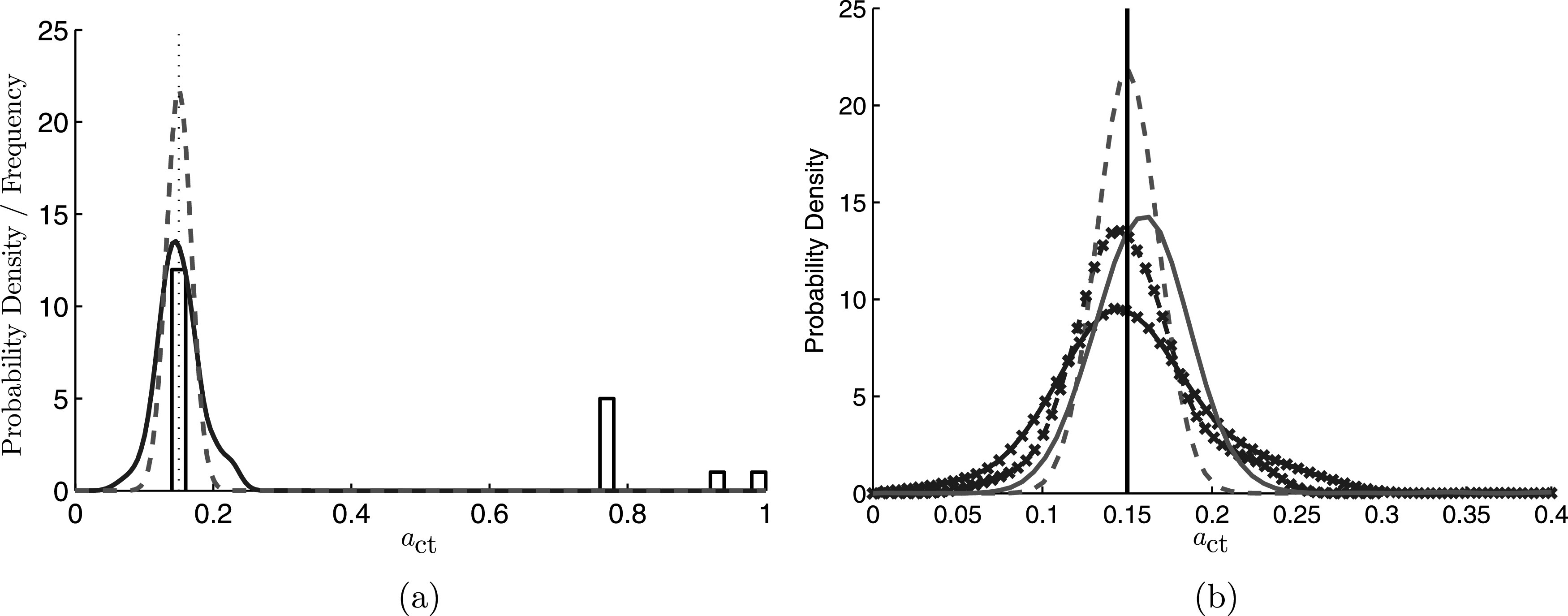
(Color online) (a) Estimated posterior distributions of computed with: the current non-stationary particle filter method (dashed line); the stationary importance sampling method (solid line); and the least squares Nelder-Mead algorithm (histogram). The histogram is the frequency of estimated computed from the 20 random seeds. The true value is marked by the dotted line. (b) Estimated posterior distributions of computed using the current non-stationary particle filter method (no symbols) and the stationary importance sampling method (symbols) for two levels of measurement noise. Dashed lines correspond to 5% additive Gaussian random noise, while solid lines correspond to 10% noise.
TABLE I.
Summary statistics of the particle filter and importance sampling estimates of the stationary muscle activation parameter , when the simulated measurements are corrupted by 5% and 10% noise. The credibility interval limits are for 95% confidence.
| 5% Noise | 10% Noise | |||
|---|---|---|---|---|
| MAP | Credibility | MAP | Credibility | |
| Estimate | Interval | Estimate | Interval | |
| Particle filter | 0.151 | (0.113, 0.186) | 0.158 | (0.091, 0.236) |
| Importance sampling | 0.145 | (0.088, 0.228) | 0.146 | (0.0519, 0.316) |
The true power of the Bayesian estimation framework is not just in the estimate itself, however, but rather in the quantification of the uncertainty in that estimate, which is illustrated by the widths of the distributions for the importance sampling and particle filter methods, which are quantified in Fig. 4(a). Such uncertainty estimates are not possible using traditional optimization based methods. The credibility intervals from the particle filter are tighter because they are computed using the full time series data, which contains more information about than a single fundamental frequency measurement; hence, there is less uncertainty in the estimated value of . We note that the improved credibility bounds come at the cost of significantly increased computational effort, however, and may not be worth the expense when it is known that a parameter does not change with time.
Figure 4(b) illustrates the impact of increased measurement uncertainty on both the importance sampling method of Cataldo et al., as well as the current particle filter scheme by artificially increasing the noise in the observed data. Specifically, the posterior densities are compared for these two techniques wherein the input glottal area waveform has been corrupted by 5% and 10% Gaussian random noise. As expected, increasing the noise of the input signal results in broader peaks of the posterior densities for both of the estimation procedures. Specifically, the credibility intervals increase by approximately 38% when doubling the noise in the observed data. The particle filter technique still provides tighter credibility intervals when compared to the importance sampling approach due to the increased information present in the time-varying signal.
B. Results and discussion for time varying
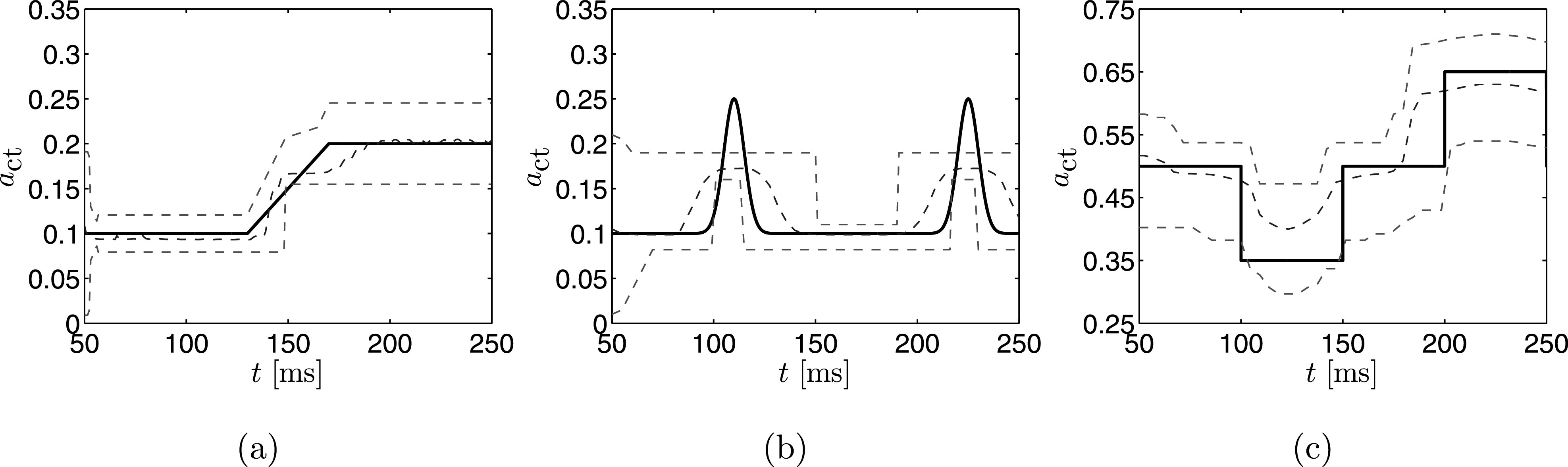
While all three techniques are reasonably successful at estimating from observation data in which that parameter is constant over time, the advantage of the particle filter method is highlighted when performing non-stationary parameter estimation. As a demonstration, we consider three additional sets of observed data. The first is generated using the BCM with initially set at 0.1 for the first 130 ms of the simulation, followed by a linear ramp to 0.2 over the next 40 ms, then held steady at 0.2 for the final 80 ms, see Fig. 5(a). The generated glottal area time series is presented in Fig. 5(d). The second set of observed data is generated with at a base value of 0.1 then exhibiting two smooth peaks rising to 0.25 and falling back to the base level. These peaks occur at and , see Fig. 5(b). The generated glottal area time series is presented in Fig. 5(e). Finally, the third simulation has a baseline of 0.5 with a drop down to 0.35 occurring at 100 ms and sustaining for 50 ms, and then a rise to 0.65 occurring at 200 ms which sustains for 50 ms. See Fig. 5(c) for the and Fig. 5(f) for the corresponding glottal waveform.
FIG. 5.

(Color online) (a)–(c) The time varying used in the three simulations. (d)–(f) Simulated time series of glottal area waveform resulting from the different time series.
All other simulation parameters for these non-stationary data sets are the same as for the stationary simulation; that is, , and . Again, the glottal area time series have been shifted so that the closure of the masses corresponds to a glottal area of 0, though there is a non-zero PGO. The particle filter uses 300 random samples at each time step to estimate the distribution. Also, the state and observation noise models were chosen to be Gaussian and unbiased, and have a standard deviation equivalent to 5% of the maximal value of the simulated state and observations, as for the time-invariant case.
Figure 6 presents time series of the MAP estimates and associated mass displacements as determined using the proposed particle filter method with the observed data in Figs. 5(d)–5(f). Analogous to the results for a constant presented in Fig. 3, the estimates of fluctuate about the true value with tight credibility intervals, except during vocal fold collision. In all cases we see that even when these collisions occur the MAP estimate continues to track the true time series, only the credibility intervals are affected by the collisions. When there is no collision the width of the credibility intervals is approximately 0.06 for all simulations. Table II summarizes the estimates at 70, 150, and 230 ms. We note that in all cases the true value of falls within the estimated credibility bounds.
FIG. 6.
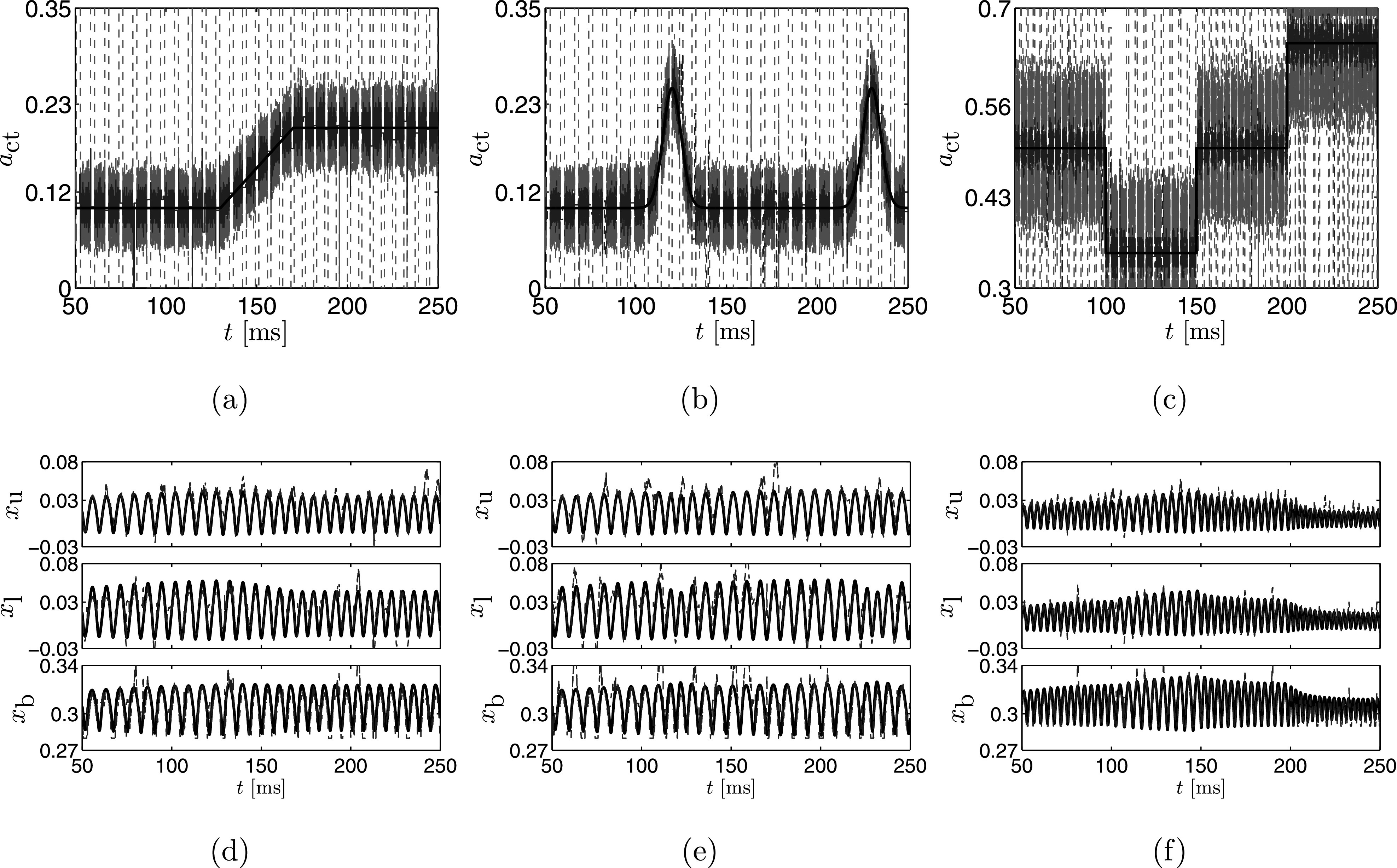
(Color online) (a)–(c) show the time series of the MAP estimate computed using the particle filter (dashed line) and the associated credibility bounds for each time step (dashed line) for the three cases. The true value for is the solid line. (d)–(f) Time series of the mass displacement MAP estimates computed using the particle filter (dashed line) and the true displacement of the masses is the solid line.
TABLE II.
Three non-stationary estimates for 70, 150, and 230 ms. The bold number is the true value, the italicized interval is the 95% credibility interval, and the normal text is the MAP estimate.
| Simulation (a) | Simulation (b) | Simulation (c) | |
|---|---|---|---|
| Estimate | 0.101, 0.1 | 0.098, 0.1 | 0.501, 0.5 |
| at 70 ms | |||
| Estimate | 0.135, 0.15 | 0.106, 0.1 | 0.315, 0.35 |
| at 150 ms | |||
| Estimate | 0.189, 0.2 | 0.265, 0.25 | 0.661 (0.65) |
| at 230 ms |
Importantly, the variation of with time is accurately captured. Over time, the evolution of is accurately captured in both simulations and the mean squared error due to the noisy nature of the MAP estimate is between 0.012 and 0.022 for all cases. The displacements of the masses are well-estimated, with the best accuracy for the upper mass, as was the case for the stationary estimation. Again we see that the body mass is the most poorly estimated. This reduction of accuracy could be due to the fact that displacement of the body mass can be approximated by a correlated change in the displacement of both the upper and lower masses. More work is required to investigate whether the accuracy of xb improves with additional measurements, such as electroglottography, or by improving model fidelity.
To elucidate how the state and observation noise impacts the estimates, the three simulation cases were run for combinations of state and observation noise variances. Table III summarizes how increasing the various noise conditions influences the accuracy of the estimate in terms of the mean squared error of the MAP estimates, and the average width of the estimated credibility interval. Table III shows that no matter the source of the noise, whether state or observation, as the noise increases the MAP estimate becomes less accurate on average and the credibility intervals grow wider. The reduction in accuracy of the MAP estimate with the increasing noise model indicates that a wider combination of parameters fits the observation data well. This means that the noisy nature of the particle filter will be exaggerated since a greater variety of particles are now acceptable. The credibility intervals widen since the greater noise level means we are less certain about the estimated value of . We also find that when the state noise is increased the error in the MAP estimate is primarily affected, whereas, when the observation noise is increased the credibility intervals are primarily affected. This occurs because the state noise is directly related to the propagation of the estimate through the evolution model, and the observation noise affects the goodness of fit.
TABLE III.
The root-mean-squared error (normal text) and width of the 95% credibility intervals (bold text) for the different noise models.
| State noise 5% | State noise 10% | State noise 5% | |
|---|---|---|---|
| Observation noise 5% | Observation noise 5% | Observation noise 10% | |
| Simulation | 0.0126 | 0.0291 | 0.0187 |
| (a) | 0.0594 | 0.0654 | 0.0871 |
| Simulation | 0.0182 | 0.027 | 0.0243 |
| (b) | 0.0595 | 0.0623 | 0.0855 |
| Simulation | 0.0223 | 0.0315 | 0.0288 |
| (c) | 0.0612 | 0.0713 | 0.082 |
1. Estimation using importance sampling and Nelder-Mead
In order to estimate using the importance sampling and Nelder-Mead methods, we must assess the fundamental frequency of the glottal area signal; however, since varies in time, so too does the fundamental frequency. In order to facilitate estimation using these methods, we estimate the fundamental frequency at each time tk through a fast Fourier transform (FFT). This produces a time series of the fundamental frequency shown in Fig. 7.
FIG. 7.
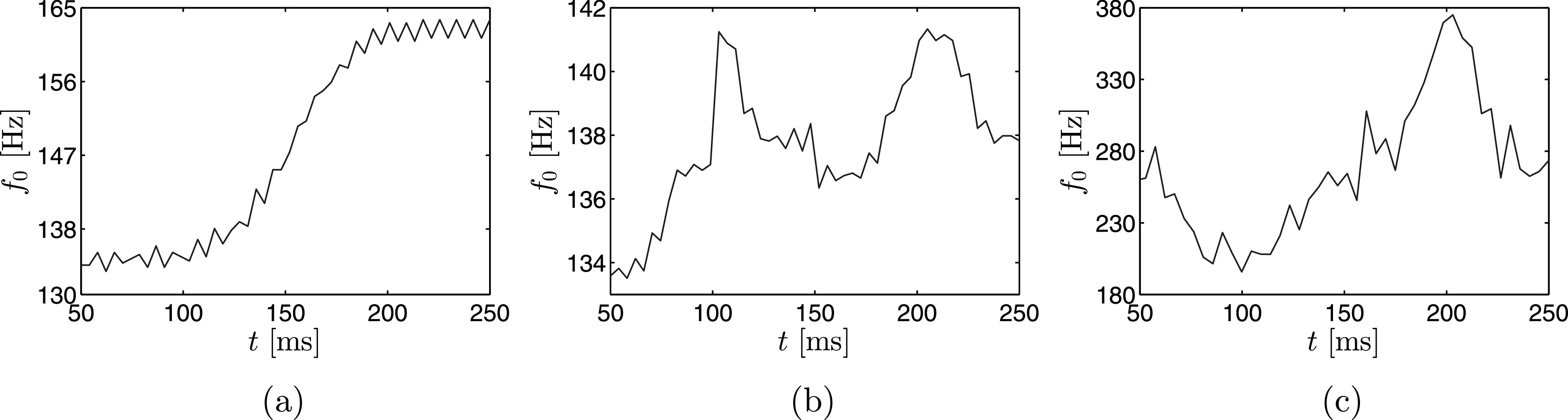
(Color online) The fundamental frequency time series from an FFT of the glottal area time series for the first case, shown in Figs. 6(d)–6(f).
Estimates for computed using importance sampling are shown in Figs. 8(a)–8(c), and those computed using Nelder-Mead are shown in Figs. 8(d)–8(f). For all test cases, the importance sampling method quickly converges to the initial value of , but is unable to follow the value of as it changes in time. The credibility bounds are initially large, as only a small amount of data has been used to estimate the fundamental frequency and, as such, there is a high degree of uncertainty surrounding the value. At approximately 100 ms in the first simulation, sufficient information is obtained from the measurement data to shrink the estimated credibility bounds. However, once the value of begins to change, uncertainty of the fundamental frequency increases and the credibility bounds respond accordingly.
FIG. 8.
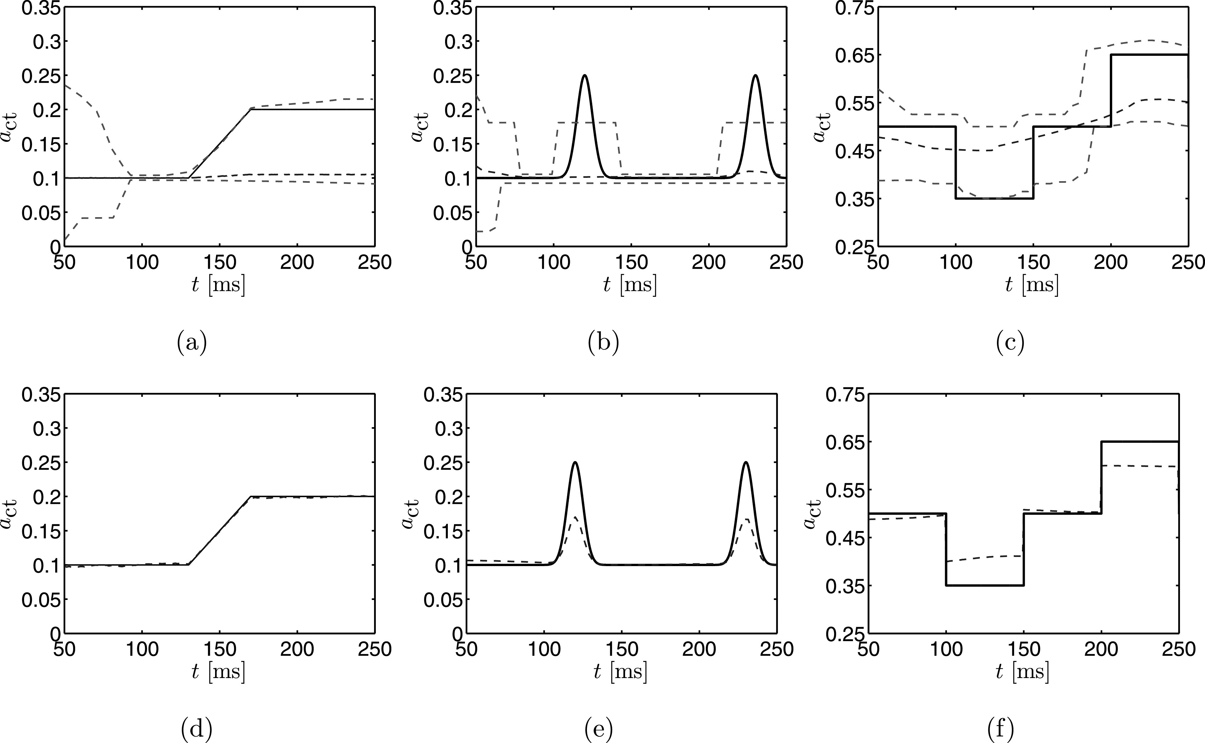
(Color online) (a)–(c) Estimates for the three test cases when the importance sampling method is used. (d)–(f) Estimates for the three cases when the Nelder-Mead method is used. The dashed lines are the time series of estimated by each respective technique, while the solid line corresponds to the true value. Bounding dashed lines in (a)–(c) are the credibility bounds.
A similar pattern occurs for the second test case. At first the credibility bounds shrink as measurements are added to the inference procedure, but then the change in causes the level of uncertainty to increase again. Also, there is a slight rise in the MAP estimate. This rise is damped because the entire history up to the given time is considered in the estimation, causing the peak to be missed. After the first peak the estimate and credibility bounds shrink once again, but the estimate of is larger than before the first peak, since this rise is now in the fundamental frequency history. Finally, the last rise is missed in the MAP estimate but the credibility bounds expand due to the change. The poor performance of the importance sampling method occurs since the fundamental frequency measure is computed from the entire history of the glottal area time series. As a result, the estimation process cannot detect the increases in and greater uncertainty in the estimates is induced.
The estimates of the third test case show too much uncertainty for any useful inference to be made at all times. The general fall and rise over time are captured but the actual structure in the time series is completely missed. Moreover, the uncertainty never decreases as in other simulations. This is likely due to the difference in the over activation of the tissue making the oscillations more frequent in the glottal area. This makes it harder to infer anything from the fundamental frequency.
The Nelder-Mead estimate for the first case in Fig. 8(d) appears very accurate, with all plotted estimates within 0.001 of the true value; however, care must be taken in interpreting these results, as the estimate which provides the lowest RMS out of the 20 seeds for each time step is plotted. The other random seeds had varying performance; around 40% of the seeds for each time step estimate to be above 0.5. As discussed previously, the most important aspect, however, is that there is no way to comment on the uncertainty surrounding such an estimate.
The estimate for the second and third cases, shown in Figs. 8(e) and 8(f), respectively, captures the changes in better than the importance sampling approach, but are unable to accurately capture the peaks of the changes. This may be due to the fact that the changes are rapid in comparison to the first simulation, and the history of the fundamental frequency has a similar damping effect as observed for the importance sampling estimates.
2. Revisiting importance sampling
An obvious strategy to improve the importance sampling method to estimate non-stationary parameters is to employ a running average (or windowing) of the time-varying observation data, as opposed to its entire time history. This technique was explored by taking FFTs of sequential 50 ms segments of the time series data from the simulation shown in Figs. 5(d)–5(f) to compute the “instantaneous” fundamental frequency for use as the measure in the importance sampling method. The resulting estimate and uncertainty bounds are shown in Fig. 9.
FIG. 9.
(Color online) The true time series (solid line) plotted with the MAP estimate (dashed line) and 95% credibility bounds (dashed line) computed using importance sampling when the fundamental frequency measure is computed using a moving time window for the three time varying simulations.
During the initial phase of the first case, when the true value of is constant at 0.1, the estimated value is relatively close to the actual value. The estimate is not as accurate as when using the full measurement history, however, due to the reduced information content available for the estimation process. The estimated value deviates from the actual value when the latter is changing in time in the linear transition region from to 0.2, but again provides a decent estimation when the value of is constant in time. This is in contrast to the estimation employing the full time history in Fig. 8(a), wherein the estimation procedure was inaccurate once began varying in time. The credibility limits are initially wide, and then tighten to a fixed width leading up to the transition region. The limits are fixed in width due to the limited information available in the window, whereas the credibility intervals continually tighten in this region when using the full time history. In the linear transition region the credibility intervals fluctuate before obtaining a fixed value again once is again constant.
The windowed importance sampling approach was able to detect both increases in for the second case, see Fig. 9(b). As was the case for the windowed estimate of the first case, the uncertainty bounds are significantly wider than those obtained from the full measurement history. Furthermore, the peaks of the rises are not completely estimated; this is likely due to the windowed nature of the estimate. That is, the peak is damped due to the lower values before and after the peak being included in the window. This behavior is similar in the third simulation. The estimate in Fig. 9(c) locates the decrease and increase in , but does not quite reach the full peaks.
In general, the windowed estimates are a considerable improvement over the importance sampling scheme which employs the full time history [Figs. 8(a)–8(c)]. If windowing is applied to compute the fundamental frequency, then the importance sampling method is able to track changes in , though with considerably less accuracy during transient regions of the observation when compared to the estimates computed with the particle filter approach. This uncertainty would be reduced when more particles are used to estimate the distribution, however, this comes with an increased computational cost. For time-variant property estimation we recommend the proposed particle filtering method.
V. CONCLUSIONS
Bayesian estimation is a powerful framework for inferring model parameters and their associated uncertainties using observed data and available a priori knowledge of the parameters. To date, the Bayesian framework had only been applied to estimate vocal fold parameters that do not change with time; this condition is encountered in, for example, sustained vowel phonation. However, during more complex vocal gestures, model parameters have to vary in time in order to capture the observed phenomena.
In this manuscript we introduced the Bayesian framework using a particle filter technique for estimating time-varying parameters in a vocal fold model. The particle filter was used to estimate parameters which are constant, as well as those which vary over time, from simulated glottal area data corrupted by Gaussian noise. In all cases, the particle filter gave accurate estimates with tight credibility bounds, except when the vocal folds were colliding, wherein the credibility bounds became quite large. This was due to the paucity of information in the observed data during collision; that is, the glottal area is during collision, the information content is dramatically reduced, causing increased uncertainty in the measurement.
Performance of the particle filter method was assessed through comparison with the importance sampling method employed by Cataldo et al.36 and the Nelder-Mead algorithm used to minimize a least squares functional, which has been used for model parameter inference in speech.24 The latter method provides only an estimate of the parameter value, but no information regarding confidence in that estimation. All methods accurately estimated the parameter value when it was stationary (i.e., when the synthetic observation data were generated using a parameter that was constant over time), with the particle filter estimating the closest value. In addition, the credibility intervals were tightest for the particle filter method, as more information from the observation data were employed in the estimation process. This came at the cost of additional computational expense, however.
In the case of synthetic data constructed using time-varying parameters, the particle filter was again successful at inferring the unknown, now time-varying, model parameter. How the state and observation noise models affect the particle filter estimates was examined and, as expected, we found that as the noise increased, no matter the source, the quality of the estimates decreased and the uncertainty, in the form of an estimated credibility interval, increased. In contrast, the importance sampling technique was unable to track the variations in the parameters, as this technique was sensitive to the time history of the observed data. Modifying this method to use only observation data from moving windows as opposed to the full time history improved the estimation of time-varying parameters, though estimates were still poor when the parameter was changing rapidly, and the confidence bounds were wide. The least-squares method was able to accurately capture and track the temporal variations in the unknown parameter when the variation was slow; however, being a non-stochastic estimation, it provided no uncertainty information making it hard to assess the appropriateness of any single estimate. This latter method also struggled with rapid changes in the value of the inferred parameter.
This first implementation of particle filters to estimate time-varying parameters in reduced order models of speech shows good promise as a tool for ultimately developing patient-specific vocal fold models. To reach this goal, further work is required to include more model complexities, such as turbulence and asymmetric tissue properties, along with clinical data and the associated uncertainties into the estimation process. Through the Bayesian framework, these uncertainties propagate into the parameter estimations and model predictions, providing quantitative evaluations of model quality. Furthermore, Bayesian estimation can provide insight into appropriate model complexity and guide model selection, which will be critical information for clinicians looking to models to aid in diagnosis and treatment decisions.
ACKNOWLEDGMENTS
P.J.H. was supported, in part, through S.D.P.'s Early Researcher Award from the Ontario Ministry of Research and Innovation (Grant No. ER13-09-269). G.E.G. acknowledges the support of CONICYT and UTFSM doctoral grants, and MESESUP (Grant No. FSM1204), M.Z. acknowledges support from CONICYT Grant Nos. FONDECYT 1151077 and BASAL FB0008, and E.C. thanks FAPERJ, CNPq, and CAPES (Grant No. BEX 2623/15-3). We would also like to thank Professor Juan Yuz for his assistance with the state space model discretization.
References
- 1. Titze I. R., “ Parameterization of the glottal area, glottal flow, and vocal fold contact area,” J. Acoust. Soc. Am. 75, 570–580 (1984). 10.1121/1.390530 [DOI] [PubMed] [Google Scholar]
- 2. Ishizaka K. and Flanagan J. L., “ Synthesis of voiced sounds from a two-mass model of the vocal cords,” Bell System Tech. J. 51, 1233–1268 (1972). 10.1002/j.1538-7305.1972.tb02651.x [DOI] [Google Scholar]
- 3. Story B. H., “ Physiologically-based speech simulation using an enhanced wave-reflection model of the vocal tract,” Ph.D. thesis, University of Iowa; (1995). [Google Scholar]
- 4. Steinecke I. and Herzel H., “ Bifurcations in an asymmetric vocal-fold model,” J. Acoust. Soc. Am. 97, 1874–1884 (1995). 10.1121/1.412061 [DOI] [PubMed] [Google Scholar]
- 5. Titze I. R. and Story B. H., “ Rules for controlling low-dimensional vocal fold models with muscle activation,” J. Acoust. Soc. Am. 112, 1064–1076 (2002). 10.1121/1.1496080 [DOI] [PubMed] [Google Scholar]
- 6. Jiang J. J., Diaz C. E., and Hanson D. G., “ Finite element modeling of vocal fold vibration in normal phonation and hyperfunctional dysphonia: Implications for the pathogenesis of vocal nodules,” Annals Otol., Rhinol., Laryngol. 107, 603–610 (1998). 10.1177/000348949810700711 [DOI] [PubMed] [Google Scholar]
- 7. Zhao W., Zhang C., Frankel S. H., and Mongeau L., “ Computational aeroacoustics of phonation, part i: Computational methods and sound generation mechanisms,” J. Acoust. Soc. Am. 112, 2134–2145 (2002). 10.1121/1.1506693 [DOI] [PubMed] [Google Scholar]
- 8. Tao C., Jiang J. J., and Zhang Y., “ Simulation of vocal fold impact pressures with a self-oscillating finite-element model,” J. Acoust. Soc. Am. 119, 3987–3994 (2006). 10.1121/1.2197798 [DOI] [PubMed] [Google Scholar]
- 9. Tao C., Jiang J. J., and Zhang Y., “ Anterior-posterior biphonation in a finite-element model of vocal fold vibration,” J. Acoust. Soc. Am. 120, 1570–1577 (2006). 10.1121/1.2221546 [DOI] [PubMed] [Google Scholar]
- 10. Zheng X., Mittal R., and Bielamowicz S., “ A computational study of asymmetric glottal jet deflection during phonation,” J. Acoust. Soc. Am. 129, 2133–2143 (2011). 10.1121/1.3544490 [DOI] [PMC free article] [PubMed] [Google Scholar]
- 11. Zheng X., Mittal R., Xue Q., and Bielamowicz S., “ Direct-numerical simulation of the glottal jet and vocal-fold dynamics in a three-dimensional laryngeal model,” J. Acoust. Soc. Am. 130, 404–415 (2011). 10.1121/1.3592216 [DOI] [PMC free article] [PubMed] [Google Scholar]
- 12. Mittal R., Erath B. D., and Plesniak M. W., “ Fluid dynamics of human phonation and speech,” Ann. Rev. Fluid Mech. 45, 437–467 (2013). 10.1146/annurev-fluid-011212-140636 [DOI] [Google Scholar]
- 13. Erath B. D., Zañartu M., Stewart K. C., Plesniak M. W., Sommer D. E., and Peterson S. D., “ A review of lumped-element models of voiced speech,” Speech Commun. 55, 667–690 (2013). 10.1016/j.specom.2013.02.002 [DOI] [Google Scholar]
- 14. Berry D. A., Herzel H., Titze I. R., and Krischer K., “ Interpretation of biomechanical simulations of normal and chaotic vocal fold oscillations with empirical eigenfunctions,” J. Acoust. Soc. Am. 95, 3595–3604 (1994). 10.1121/1.409875 [DOI] [PubMed] [Google Scholar]
- 15. Titze I. R., “ Nonlinear source–filter coupling in phonation: Theory,” J. Acoust. Soc. Am. 123, 2733–2749 (2008). 10.1121/1.2832337 [DOI] [PMC free article] [PubMed] [Google Scholar]
- 16. Zañartu M., Mongeau L., and Wodicka G. R., “ Influence of acoustic loading on an effective single mass model of the vocal folds,” J. Acoust. Soc. Am. 121, 1119–1129 (2007). 10.1121/1.2409491 [DOI] [PubMed] [Google Scholar]
- 17. Ho J. C., Zañartu M., and Wodicka G. R., “ An anatomically based, time-domain acoustic model of the subglottal system for speech production,” J. Acoust. Soc. Am. 129, 1531–1547 (2011). 10.1121/1.3543971 [DOI] [PubMed] [Google Scholar]
- 18. Story B. H. and Titze I. R., “ Voice simulation with a body-cover model of the vocal folds,” J. Acoust. Soc. Am. 97, 1249–1260 (1995). 10.1121/1.412234 [DOI] [PubMed] [Google Scholar]
- 19. Alku P., Magi C., Yrttiaho S., Bäckström T., and Story B., “ Closed phase covariance analysis based on constrained linear prediction for glottal inverse filtering,” J. Acoust. Soc. Am. 125, 3289–3305 (2009). 10.1121/1.3095801 [DOI] [PubMed] [Google Scholar]
- 20. Kuo H. J., “ Voice source modeling and analysis of speakers with vocal fold nodules,” Ph.D. thesis, Massachusetts Institute of Technology; (1998). [Google Scholar]
- 21. Zhang Y., McGilligan C., Zhou L., Vig M., and Jiang J. J., “ Nonlinear dynamic analysis of voices before and after surgical excision of vocal polyps,” J. Acoust. Soc. Am. 115, 2270–2277 (2004). 10.1121/1.1699392 [DOI] [PubMed] [Google Scholar]
- 22. Horáček J., Šidlof P., and Švec J., “ Numerical simulation of self-oscillations of human vocal folds with hertz model of impact forces,” J. Fluids Struct. 20, 853–869 (2005). 10.1016/j.jfluidstructs.2005.05.003 [DOI] [Google Scholar]
- 23. Zañartu M., Galindo G. E., Erath B. D., Peterson S. D., Wodicka G. R., and Hillman R. E., “ Modeling the effects of a posterior glottal opening on vocal fold dynamics with implications for vocal hyperfunction,” J. Acoust. Soc. Am. 136, 3262–3271 (2014). 10.1121/1.4901714 [DOI] [PMC free article] [PubMed] [Google Scholar]
- 24. Döllinger M., Hoppe U., Hettlich F., Lohscheller J., Schuberth S., and Eysholdt U., “ Vibration parameter extraction from endoscopic image series of the vocal folds,” IEEE Trans. Biomed. Eng. 49, 773–781 (2002). 10.1109/TBME.2002.800755 [DOI] [PubMed] [Google Scholar]
- 25. Schwarz R., Hoppe U., Schuster M., Wurzbacher T., Eysholdt U., and Lohscheller J., “ Classification of unilateral vocal fold paralysis by endoscopic digital high-speed recordings and inversion of a biomechanical model,” IEEE Trans. Biomed. Eng. 53, 1099–1108 (2006). 10.1109/TBME.2006.873396 [DOI] [PubMed] [Google Scholar]
- 26. Wurzbacher T., Schwarz R., Döllinger M., Hoppe U., Eysholdt U., and Lohscheller J., “ Model-based classification of nonstationary vocal fold vibrations,” J. Acoust. Soc. Am. 120, 1012–1027 (2006). 10.1121/1.2211550 [DOI] [PubMed] [Google Scholar]
- 27. Schwarz R., Döllinger M., Wurzbacher T., Eysholdt U., and Lohscheller J., “ Spatio-temporal quantification of vocal fold vibrations using high-speed videoendoscopy and a biomechanical model,” J. Acoust. Soc. Am. 123, 2717–2732 (2008). 10.1121/1.2902167 [DOI] [PubMed] [Google Scholar]
- 28. Cataldo E., Soize C., Sampaio R., and Desceliers C., “ Probabilistic modeling of a nonlinear dynamical system used for producing voice,” Computat. Mech. 43, 265–275 (2009). 10.1007/s00466-008-0304-0 [DOI] [Google Scholar]
- 29. Rupitsch S. J., Ilg J., Sutor A., Lerch R., and Döllinger M., “ Simulation based estimation of dynamic mechanical properties for viscoelastic materials used for vocal fold models,” J. Sound Vib. 330, 4447–4459 (2011). 10.1016/j.jsv.2011.05.008 [DOI] [Google Scholar]
- 30. Yang A., Berry D. A., Kaltenbacher M., and Döllinger M., “ Three-dimensional biomechanical properties of human vocal folds: Parameter optimization of a numerical model to match in vitro dynamics,” J. Acoust. Soc. Am. 131, 1378–1390 (2012). 10.1121/1.3676622 [DOI] [PMC free article] [PubMed] [Google Scholar]
- 31. Wurzbacher T., Döllinger M., Schwarz R., Hoppe U., Eysholdt U., and Lohscheller J., “ Spatiotemporal classification of vocal fold dynamics by a multimass model comprising time-dependent parameters,” J. Acoust. Soc. Am. 123, 2324–2334 (2008). 10.1121/1.2835435 [DOI] [PubMed] [Google Scholar]
- 32. Tao C., Zhang Y., and Jiang J. J., “ Extracting physiologically relevant parameters of vocal folds from high-speed video image series,” IEEE Trans. Biomed. Eng. 54, 794–801 (2007). 10.1109/TBME.2006.889182 [DOI] [PubMed] [Google Scholar]
- 33. Zhang Y., Tao C., and Jiang J. J., “ Parameter estimation of an asymmetric vocal-fold system from glottal area time series using chaos synchronization,” Chaos 16, 023118 (2006). 10.1063/1.2203092 [DOI] [PubMed] [Google Scholar]
- 34. Yang A., Stingl M., Berry D. A., Lohscheller J., Voigt D., Eysholdt U., and Döllinger M., “ Computation of physiological human vocal fold parameters by mathematical optimization of a biomechanical model,” J. Acoust. Soc. Am. 130, 948–964 (2011). 10.1121/1.3605551 [DOI] [PMC free article] [PubMed] [Google Scholar]
- 35. Kaipio J. and Somersalo E., Statistical and Computational Inverse Problems ( Springer-Verlag, New York, 2005), pp. 1–340. [Google Scholar]
- 36. Cataldo E., Soize C., and Sampaio R., “ Uncertainty quantification of voice signal production mechanical model and experimental updating,” Mech. Syst. Signal Process. 40, 718–726 (2013). 10.1016/j.ymssp.2013.06.036 [DOI] [Google Scholar]
- 37. Hillman R. E., Holmberg E. B., Perkell J. S., Walsh M., and Vaughan C., “ Objective assessment of vocal hyperfunction: An experimental framework and initial results,” J. Speech, Lang., Hear. Res. 32, 373–392 (1989). 10.1044/jshr.3202.373 [DOI] [PubMed] [Google Scholar]
- 38. Bowen L. K., Hands G. L., Pradhan S., and Stepp C. E., “ Effects of Parkinson's disease on fundamental frequency variability in running speech,” J. Med. Speech-Lang. Pathol. 21, 235–244 (2013). [PMC free article] [PubMed] [Google Scholar]
- 39. Rahn D. A., Chou M., Jiang J. J., and Zhang Y., “ Phonatory impairment in Parkinson's disease: Evidence from nonlinear dynamic analysis and perturbation analysis,” J. Voice 21, 64–71 (2007). 10.1016/j.jvoice.2005.08.011 [DOI] [PubMed] [Google Scholar]
- 40. Jiang J. J., Zhang Y., and McGilligan C., “ Chaos in voice, from modeling to measurement,” J. Voice 20, 2–17 (2006). 10.1016/j.jvoice.2005.01.001 [DOI] [PubMed] [Google Scholar]
- 41. Liu J., Monte Carlo Strategies in Scientific Computing ( Springer, New York, 2004), pp. 1–344. [Google Scholar]
- 42. Bernardo J. and Smith A., “ Bayesian theory,” in Wiley Series in Probability and Statistics ( John Wiley & Sons, West Sussex, England, 2000), pp. 1–610. [Google Scholar]
- 43. Smith A. F. M. and Gelfand A. E., “ Bayesian statistics without tears: A sampling-resampling perspective,” Am. Statistician 46, 84–88 (1992). 10.1080/00031305.1992.10475856 [DOI] [Google Scholar]
- 44. Jones M. C., Marron J. S., and Sheather S. J., “ A brief survey of bandwidth selection for density estimation,” J. Am. Stat. Assoc. 91, 401–407 (1996). 10.1080/01621459.1996.10476701 [DOI] [Google Scholar]
- 45. Kaipio J. and Somersalo E., “ Statistical inverse problems: Discretization, model reduction and inverse crimes,” J. Comput. Appl. Math. 198, 493–504 (2007). 10.1016/j.cam.2005.09.027 [DOI] [Google Scholar]
- 46. Cappé O., Moulines E., and Ryden T., Inference in Hidden Markov Models, Springer Series in Statistics ( Springer-Verlag, New York, 2005), pp. 1–653. [Google Scholar]
- 47. Gordon N., Salmond D., and Smith A., “ Novel approach to nonlinear/non-Gaussian Bayesian state estimation,” IEEE Proc. Radar Signal. Process. 140, 107–113 (1993). 10.1049/ip-f-2.1993.0015 [DOI] [Google Scholar]
- 48. Omori K., Slavit D. H., Kacker A., and Blaugrund S. M., “ Influence of size and etiology of glottal gap in glottic incompetence dysphonia,” Laryngoscope 108, 514–518 (1998). 10.1097/00005537-199804000-00010 [DOI] [PubMed] [Google Scholar]
- 49. Södersten M. and Lindestad P. A., “ Glottal closure and perceived breathiness during phonation in normally speaking subjects,” J. Speech Hear. Res. 33, 601–611 (1990). 10.1044/jshr.3303.601 [DOI] [PubMed] [Google Scholar]
- 50. Chen G., Kreiman J., Shue Y.-L., and Alwan A., “ Acoustic correlates of glottal gaps,” Interspeech 4, 2684–2687 (2011). [Google Scholar]
- 51. Linville S. E., “ Glottal gap configurations in two age groups of women,” J. Speech, Lang., Hear. Res. 35, 1209–1215 (1992). 10.1044/jshr.3506.1209 [DOI] [PubMed] [Google Scholar]
- 52. Hanson H. M., “ Glottal characteristics of female speakers: Acoustic correlates,” J. Acoust. Soc. Am. 101, 466–481 (1997). 10.1121/1.417991 [DOI] [PubMed] [Google Scholar]
- 53. Story B. H. and Bunton K., “ Production of child-like vowels with nonlinear interaction of glottal flow and vocal tract resonances,” Proc. Meet. Acoust. 19, 060303 (2013). 10.1121/1.4798416 [DOI] [Google Scholar]
- 54. Švec J. G. and Schutte H. K., “ Videokymography: High-speed line scanning of vocal fold vibration,” J. Voice 10, 201–205 (1996). 10.1016/S0892-1997(96)80047-6 [DOI] [PubMed] [Google Scholar]
- 55. Takemoto H., Honda K., Masaki S., Shimada Y., and Fujimoto I., “ Measurement of temporal changes in vocal tract area function from 3D cine-MRI data,” J. Acoust. Soc. Am. 119, 1037–1049 (2006). 10.1121/1.2151823 [DOI] [PubMed] [Google Scholar]
- 56. McGowan R. S., “ An aeroacoustic approach to phonation,” J. Acoust. Soc. Am. 83, 696–704 (1988). 10.1121/1.396165 [DOI] [PubMed] [Google Scholar]
- 57. Deliyski D. and Petrushev P., “ Methods for objective assessment of high-speed videoendoscopy,” in Proceedings of the 6th International Conference: Advances in Quantitative Laryngology, Voice and Speech Research, AQL-2003, Hamburg, Germany (April 2003), pp. 1–16. [Google Scholar]
- 58. Galindo G. E., Zañartu M., and Yuz J. I., “ A discrete-time model for the vocal folds,” in IEEE EMBS International Student Conference, Chile (2014), pp. 74–77. [Google Scholar]
- 59. Jaynes E. T., “ Information theory and statistical mechanics,” Phys. Rev. 106, 620–630 (1957). 10.1103/PhysRev.106.620 [DOI] [Google Scholar]
- 60. Jaynes E. T., “ Information theory and statistical mechanics. II,” Phys. Rev. 108, 171–190 (1957). 10.1103/PhysRev.108.171 [DOI] [Google Scholar]
- 61. Cover T. and Thomas J., Elements of Information Theory ( John Wiley & Sons, Inc., Hoboken, NJ, 2006), pp. 1–776. [Google Scholar]
- 62. Nocedal J. and Wright S. J., Numerical Optimization, 2nd ed. ( Springer, New York, 2006). [Google Scholar]