KS-CMI: A circRNA-miRNA interaction prediction method based on the signed graph neural network and denoising autoencoder

Summary

Circular RNA (circRNA) plays an important role in the diagnosis, treatment, and prognosis of human diseases. The discovery of potential circRNA-miRNA interactions (CMI) is of guiding significance for subsequent biological experiments. Limited by the small amount of experimentally supported data and high randomness, existing models are difficult to accomplish the CMI prediction task based on real cases. In this paper, we propose KS-CMI, a novel method for effectively accomplishing CMI prediction in real cases. KS-CMI enriches the ‘behavior relationships’ of molecules by constructing circRNA-miRNA-cancer (CMCI) networks and extracts the behavior relationship attribute of molecules based on balance theory. Next, the denoising autoencoder (DAE) is used to enhance the feature representation of molecules. Finally, the CatBoost classifier was used for prediction. KS-CMI achieved the most reliable prediction results in real cases and achieved competitive performance in all datasets in the CMI prediction.

Graphical abstract

Highlights

• •We propose a circRNA-miRNA interaction prediction method based on the balance theory
• •The model enriches association information by adding cancer molecules
• •KS-CMI allows expansion in heterogeneous graphs of binary and triplet groups

Gene network; Neural networks

Introduction

Circular RNA (circRNA) is a non-coding RNA (ncRNA) that possesses a closed-loop structure and exhibits a high degree of conservation and stability across organisms.¹ circRNA functions as the miRNA sponge and has been found to participate in a wide range of cellular processes, including cell proliferation, metastasis, and differentiation.² The potential for circRNA to function as a marker for cancer diagnosis and treatment is widely recognized and may offer new insights into the diagnosis and treatment of complex diseases.

CircRNA was first discovered in 1976,³ however, due to limited sequencing technologies and insufficient attention, only a small fraction of circRNA was unexpectedly discovered during the following three decades, which was generally regarded as background noise resulting from abnormal RNA splicing. In 2010, with the advancement of high-throughput technology and professional computing pipelines, circRNA regained its status as an important subject of biological research. CircRNAs have higher stability and a longer half-life than linear RNAs due to their unique cyclic closure structure.⁴

Recent studies have demonstrated that circRNA, as the miRNA sponge, interacts with RNA-binding protein-driven and translational proteins, thereby playing a significant regulatory role in tumor genesis and development. At the same time, the detectability of circRNA in human tissues, especially in blood, urine, saliva, and other liquid biopsy samples, makes circRNA a promising diagnostic and therapeutic marker for complex diseases. For example, hsa_circ_0000190 and has_circRNA_102958 have been identified as potential markers for gastric cancer diagnosis,⁵ hsa_circ_0001874 and hsa_circ_0001971 potential biomarkers for oral cancer diagnosis,⁶ and prostate cancer can be diagnosed by testing circPDLIM5, circSCAF8, circPLXDC2, circSCAMP1, and circCCNT2 in urine,⁷ etc. These studies demonstrate that circRNAs can provide new insights into the diagnosis and treatment of complex human diseases. As the important role of circRNA is revealed, it is necessary to explore more CMIs for circRNA-related research. Due to the limitations of labor, materials, and time, it is impractical to conduct biological experiments on all known data. With the development of computer technology, it is possible to provide the preselection range for relevant wet experiments by using calculation methods. The computational model of ncRNA-related research has been developed for nearly 10 years, resulting in many excellent models.⁸ For example, based on the assumption of functional similarity, Chen et al. integrated multiple biological networks and predicted the potential miRNA-disease associations (MDA) by calculating the within and between scores.⁹ You et al. integrated the miRNA-disease association, miRNA functional similarity, and disease semantic similarity into a heterogeneous graph, and used the path-based depth-first search algorithm to predict the MDA.¹⁰ Lei et al. presented a review on ncRNA-disease associations, which introduced miRNA, lncRNA, circRNA, and calculation methods for their associations with diseases in detail.¹¹ Zhang et al. used the association information of circRNA, miRNA, and disease to construct a weighted nuclear norm minimization model, and proposed the PDC-PGWNNM method to predict potential circRNA-disease associations.¹² Wang et al. predicted circRNA-disease association by extracting multi-source information from biological information and using the convolution neural network to extract hidden features.¹³ Guo et al. proposed the circ2CBA method, which can predict circRNA-RBP binding sites using only RNA sequences.¹⁴ Combining natural language processing and bidirectional LSTM to extract features, Wang et al. proposed a framework CRPB sites that can effectively predict the binding sites of RBP on circRNA.¹⁵ Yang et al. combined accelerated attributed network embedding to extract network features, and combined stacked autoencoder to obtain low-dimensional features and predict potential circRNA-disease associations.¹⁶

The development of circRNA research has produced a large number of data stored in different databases, such as the CircR2Disease v2.0 database,¹⁷ circBank database,¹⁸ CircR2Disease database,¹⁹ and circBase database.²⁰ These data provide conditions for the use of computational methods to pre-select CMI with high probability. At present, some methods have been tried in the field of CMI prediction, most of which are based on two commonly used datasets. Based on the data of the circBank database,²¹ Guo et al. proposed WSCD predicts potential CMI by combining natural language processing and graph embedding algorithms to obtain an AUC of 0.8898.²² Qian et al. proposed CMASG, by extracting linear and nonlinear features of molecules for CMI prediction, and obtained 0.8804 AUC.²³ He et al. proposed GCNCMI, which extracts molecular features by graph convolutional neural network and obtained the AUC of 0.9320.²⁴ Based on the CMI-9905 dataset, Wang et al. proposed the KGDCMI model, which uses neural networks for feature fusion and prediction of potential CMI by extracting sequence features and behavioral features of molecules, and finally obtained an AUC of 0.9041.²⁵ Yu et al. proposed SGCNCMI, using a graph convolutional neural network with the contribution mechanism to aggregate node information for prediction, and obtained 0.8942 AUC.²⁶ Wang et al. proposed JSNDCMI, using the sparse network multi-structure extraction framework to predict potential CMI, and obtained an AUC of 0.9003.²⁷ However, because the number of experimentally validated CMIs is too sparse, most of the data used in these methods are the predictions using Miranda²⁸ and TargetScan²⁹ techniques. Although the data used have high confidence levels and some of them have been confirmed by subsequent experiments, it also means that these models cannot be applied in real cases. There are few models for CMI prediction based on real cases. Based on the experimental data in the circR2Cancer database,³⁰ the AUC of the NECMA³¹ model is only 0.4989, which cannot complete effective prediction. The AUC of the IIMCCMA³² model is 0.6702. Although some progress has been made, the prediction effect is still uncertain.

To our knowledge, the CMI prediction in the real cases mainly has the following difficulties: (1) The data verified by experiments are scarce, and it is difficult to extract valuable information from the network built of known data. (2) The data for experimental verification mainly come from relevant literature and materials, which rely on manual addition, so they are disordered and do not have attributes like RNA sequence and others. (3) Even if valuable information about molecules can be obtained, in the training of small samples, the model lacks stability and robustness.

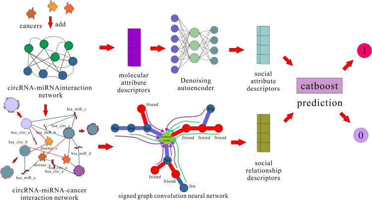
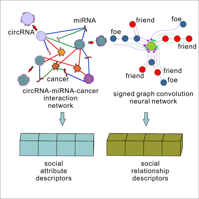
To address the above issues, we propose a new CMI prediction method, KS-CMI, which combines the balance theory in social relations and the noise reduction method in machine learning to predict the potential CMI. In detail, we reconstruct the circRNA-miRNA-cancer interaction (CMCI) network by adding cancer as an intermediary molecule in the CMI network to enrich the social relations. Next, we extract the social attribute descriptors and social relationship descriptors of molecules from the reconstructed CMCI network based on balance theory. Then, we use the denoising autoencoder³³ based on machine learning to increase the robustness of the molecular features. Finally, the CatBoost classifier³⁴ is used for training and prediction. KS-CMI achieved the AUC of 0.8132 in the prediction of real cases. In the case studies based on circ-ABCC10 and circ-ITCH, 13 out of 15 pairs of CMIs were accurately predicted. The flowchart of KS-CMI is shown in Figure 1.

Figure 1.

The flowchart of KS-CMI

Results

Evaluation criteria

In this work, we introduce the 5-fold cross-validation (5-fold CV) to test the model performance. In the 5-fold CV, the data are divided into five parts on average, one of which is not repeated and is predicted each time, and the other four parts are used as training data until the prediction score of all five parts is obtained. In addition, we have introduced several evaluation criteria, including accuracy (Acc.), precision (Prec.), and F1-score (F1), to comprehensively evaluate the performance of the model, which are calculated using the following formulas:

$$A\text{cc}.=\frac{TP+TN}{TP+TN+FP+FN}$$ (Equation 1)

$$\mathrm{Pr}ec.=\frac{TP}{TP+FP}$$ (Equation 2)

$$F1-score=\frac{2prec\times recall}{prec+recall}$$ (Equation 3)

where TP (true positive) and TN (true negative) represent the correct number of positive and negative samples predicted by the KS-CMI, respectively. FP (false positive) and FN (false negative) represent the number of positive and negative samples that the model predicts error. In addition, we plotted the receiver operating characteristic (ROC) curve and precision-recall (PR) curve of KS-CMI to clearly show the prediction results.

Performance evaluation

In this section, we performed a 5-fold CV based on the CMI-753 dataset to evaluate the performance of the KS-CMI, and the experimental results are objectively recorded in Table 1.

Table 1.

The result of the 5-fold CV in the CMI-753 dataset

Test set	Acc	Prec.	F1-score	AUC	AUPR
1	0.7517	0.7517	0.7517	0.8288	0.8218
2	0.7442	0.7447	0.7441	0.8045	0.7800
3	0.7243	0.7251	0.7243	0.8109	0.8133
4	0.6977	0.6991	0.6975	0.7928	0.7502
5	0.7608	0.7610	0.7608	0.8289	0.8028
mean	0.7357	0.7363	0.7357	0.8132	0.7936
std	±0.0225	±0.0201	±0.0205	±0.0141	±0.0259

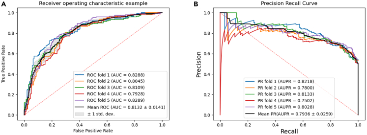
The data in Table 1 shows that the average value of KS-CMI based on the 5-fold CV in the CMI-753 dataset is 73.57%, 73.63%, 73.57%, 81.32%, and 79.36% respectively. In addition, we plotted the ROC and the PR curve of KS-CMI which is shown in Figure 2. These figures are automatically generated by the program and are reliable criteria to measure the performance of the model.

Figure 2.

AUC (a) and AUPR (b) of KS-CMI in the CMI-753 dataset

The results in Figure 2 shows that the AUC of KS-CMI in five independent experiments are 82.88%, 80.45%, 81.09%, 79.28%, and 82.89% respectively, with an average of 81.32%; The AUPR of the five experiments are 82.18%, 78.00%, 81.33%, 75.02%, and 80.28% respectively, with an average AUPR of 79.36%. These results prove that KS-CMI can effectively complete the prediction task based on the CMI-753 dataset, and is a reliable and high-precision prediction CMI model.

Comparison of different datasets

KS-CMI innovatively combined with molecular social features to predict CMI and performed well in datasets with experimental support (CMI-753). CMI-9905 and CMI-9589 are two datasets commonly used in the field of CMI prediction. At present, more than 90% of CMI prediction models use these data as benchmark data. To verify the competitiveness of KS-CMI in the field of CMI prediction, in this part, we conduct experiments based on these two common datasets. The experimental results based on CMI-9905 and CMI-9589 datasets are recorded in Tables 2 and 3 respectively.

Table 2.

The result of the 5-fold CV is based on the CMI-9905 dataset

Test set	Acc	Prec.	F1-score	AUC	AUPR
1	0.8455	0.8479	0.8453	0.9188	0.9220
2	0.8342	0.8366	0.8339	0.9080	0.9115
3	0.8281	0.8310	0.8277	0.8998	0.9101
4	0.8387	0.8410	0.8385	0.9110	0.9196
5	0.8248	0.8265	0.8246	0.9054	0.9092
mean	0.8343	0.8366	0.8340	0.9086	0.9144
std	±0.0067	±0.0068	±0.0068	±0.0063	±0.0053

Table 3.

The result of the 5-fold CV is based on the CMI-9589 dataset

Test set	Acc	Prec.	F1-score	AUC	AUPR
1	0.8329	0.8338	0.8328	0.9209	0.9241
2	0.8405	0.8411	0.8404	0.9223	0.9221
3	0.8491	0.8492	0.8490	0.9259	0.9280
4	0.8216	0.8222	0.8216	0.9076	0.9040
5	0.8310	0.8310	0.8310	0.9132	0.9125
mean	0.8350	0.8354	0.8349	0.9179	0.9181
std	±0.0084	±0.0083	±0.0084	±0.0066	±0.0087

The data in Tables 2 and 3 show that the average values of the five evaluation criteria of KS-CMI in the 5-fold CV based on the CMI-9905 dataset are 83.43%, 83.66%, 83.40%, 90.86%, and 91.44% respectively; The average values of the five evaluation criteria based on the CMI-9589 dataset are 83.50%, 83.54%, 83.49%, 91.79%, and 91.81%. The excellent results show that KS-CMI can not only complete CMI prediction based on real cases but also has an excellent performance in the data commonly used in this field. It is worth noting that the experimental results based on the CMI-9905 and CMI-9589 datasets are significantly better than the CMI-753 datasets. This is because the CMI-753 is manually collected from the existing experiments and papers. Although the data have higher reliability, they also have the characteristics of small quantity and high contingency, so the predicted performance will be affected. In addition, due to the two commonly used datasets used for comparison only having circRNA-miRNA interactions, in the comparative experiment, we extract features from binary relations, which means that the performance of the proposed model on the dataset is lower than its real level, but still achieves the most competitive results.

Performance evaluation of each part of the model

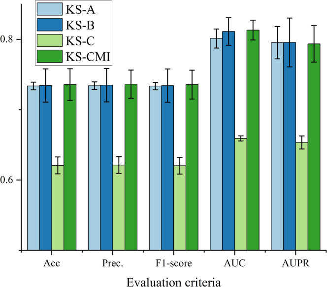
According to different functions, KS-CMI can be divided into three modules: first, KS-CMI extracts the social attribute features of molecules from the biological network (module A); then the extracted features are fused and enhanced by DAE to form the final social attribute descriptor (module B); next, the molecular social relationship descriptor is extracted by SGCN (module C). Finally, these features are sent to the classifier for the execution of downstream tasks; through the organic integration of all the modules, an efficient CMI prediction model KS-CMI is formed. In this part, we verify the effectiveness of each module of the proposed model through ablation experiments. Specifically, we remove each module in the proposed model and then keep the other conditions unchanged for the downstream prediction task, and all the experimental data are recorded in Table 4. In addition, we compare the data in Table 4 with the KS-CMI through histogram Figure 3.

Table 4.

Predicted results of KS-CMI with different modules

KS-A	Acc	Prec.	F1-score	AUC	AUPR
1	0.7252	0.7252	0.7252	0.7990	0.7937
2	0.7409	0.7412	0.7407	0.7875	0.7561
3	0.7309	0.7311	0.7308	0.8272	0.8281
4	0.7375	0.7380	0.7374	0.7932	0.8018
5	0.7342	0.7349	0.7340	0.7992	0.7968
mean	0.7337	0.7340	0.7336	0.8012	0.7953
Std	±0.0054	±0.0055	±0.0053	±0.0136	±0.0230
KS-B	Acc	Prec.	F1-score	AUC	AUPR
1	0.7252	0.7252	0.7252	0.7884	0.7341
2	0.6977	0.6981	0.6975	0.7921	0.7884
3	0.7309	0.7317	0.7306	0.8089	0.8000
4	0.7508	0.7511	0.7507	0.8289	0.8208
5	0.7674	0.7679	0.7673	0.8381	0.8348
mean	0.7344	0.7348	0.7342	0.8112	0.7956
std	±0.0236	±0.0237	±0.0237	±0.0196	±0.0347
KS-C	Acc	Prec.	F1-score	AUC	AUPR
1	0.6325	0.6326	0.6323	0.6569	0.6641
2	0.6346	0.6349	0.6342	0.6595	0.6384
3	0.6013	0.6014	0.6013	0.6649	0.6616
4	0.6179	0.6184	0.6177	0.6608	0.6485
5	0.6179	0.6196	0.6169	0.6541	0.6547
mean	0.6208	0.6213	0.6204	0.6592	0.6534
std	±0.0120	±0.0119	±0.0119	±0.0036	±0.0093

Figure 3.

Predicted performance of KS-CMI with different modules

The data in Table 4 and Figure 3 shows that the KS-CMI model performs best in all evaluation criteria, KS-B and KS-A are slightly lower than the proposed model, and KS-C is much lower than the proposed model. The conclusion shows that all modules can effectively improve the prediction performance of the model. Among all three modules, the social relationship descriptor extraction module is the module that contributes the most; DAE can effectively improve the prediction efficiency of the model with almost no loss of accuracy; Social attribute descriptors are useful complements to model features.

Evaluation of DAE effectiveness

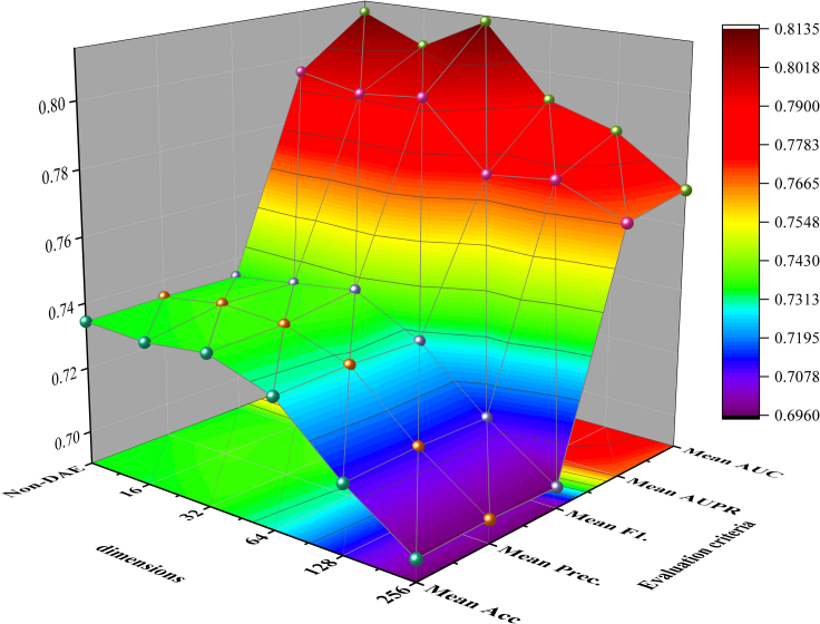
KS-CMI comprehensively considers the performance and efficiency of the model. The model should not only have good prediction accuracy but also have fast prediction speed and high robustness. To meet this challenge, we introduce DAE to learn low-dimensional feature representation. In this section, we explored the impact of DAE dimension reduction on the comprehensive performance of the model. In detail, we use DAE to learn the feature representation of different dimensions and then use the same parameters and data to conduct experiments and record the impact of different dimensions on the model. The experimental results are shown in Table 5. To facilitate comparison, we project the model performance evaluation criteria (excluding time) in the table in Figure 4.

Table 5.

Results of model extraction with different dimensions

dimensions	Acc	Prec.	F1-score	AUC	AUPR	time
Non-DAE	0.7344	0.7347	0.7342	0.8113	0.7956	109.62s
16	0.7334	0.7375	0.7368	0.8028	0.7916	53.63s
32	0.7357	0.7363	0.7395	0.8132	0.7936	59.86s
64	0.7290	0.7297	0.7288	0.7914	0.7734	75.46s
128	0.7107	0.7115	0.7110	0.7850	0.7757	108s
256	0.6965	0.6970	0.6964	0.7708	0.7670	174.84s

Figure 4.

The visualization of the Performance in Different Dimensions of the KS-CMI

The results in Table 3 and Figure 4 shows that when the DAE adopts 16-dimensional feature extraction, the model has the fastest prediction speed (53.63s), but some prediction accuracy is lost; When 256-dimensional feature extraction is used, the prediction speed of the model is even slower than that without DAE, and the prediction accuracy of the model is greatly reduced.

Considering the computing speed and efficiency, KS-CMI uses 32 dimensions as the best DAE extraction dimension. Due to the special iterative mechanism of machine learning, the low dimension may lead to the smooth transition of features, so although it improves the calculation speed, it will also affect the prediction accuracy; On the contrary, the long dimension will bring more noise, which not only increases the prediction time but also cannot effectively maintain the original value of features.

Performance comparison of signed graph neural networks

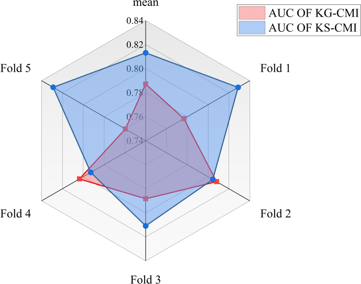
This paper proposes an efficient prediction model for CMI prediction in real cases. This model applies the balance theory in social theory to CMI biological networks through signed graph convolutional neural networks (SGCN), and effectively completes CMI in real cases predict. The SGCN used in the proposed model combines the chain of social associations based on the graph neural network, which is an extension of the graph convolutional neural network (GCN). In this part, we evaluate the superiority of SGCN. In detail, we keep other parts of the model unchanged and use GCN (KG-CMI) to perform prediction tasks in the same dataset, then we compare the KG-CMI model with the proposed model in the radar chart Figure 5 to reflect the advantages of the proposed model.

Figure 5.

Performance comparison of the proposed model

The data in Figure 5 show that in the AUC of the 5-fold cross-validation, KG-CMI is close to the proposed model with 2 folds, and the proposed model is much higher than KG-CMI in the 3-fold AUC and the average value. The experimental results show that the performance of the proposed model using SGCN is better than that of GCN. This is because SGCN has added a chain social relationship based on balance theory, which not only considers negative samples but also extracts the chain combination relationship of positive and negative samples, so SGCN performs better when targeting the same sparse dataset.

Compare with different classifiers

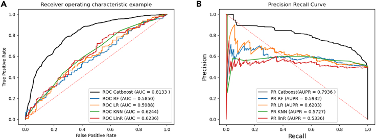
KS-CMI uses the CatBoost classifier for the training and classification task of the data. To verify the most effective classification strategy, we compare several classifiers. In detail, keeping the trained data and other conditions constant, we used Random Forest (RF),³⁵ Logistic Regression (LR),³⁶ KNN,³⁷ and Linear Regression (LinR)³⁸ to replace the CatBoost classifier in KS-CMI for a 5-fold CV, respectively, to compare the classification ability of different classifiers. The experimental results are automatically generated by the program as shown in Figure 6.

Figure 6.

Performance of KS-CMI using different classifiers

(A) for AUC comparison, (B) for AUPR comparison.

In Figure 6, the results using the CatBoost classifier are 19% higher than the second highest classifier, which may be due to the CatBoost classifier’s ability to handle multiple types of data more flexibly, and the optimization for gradient bias and prediction shift, which improves the prediction ability and robustness of the classifier. In addition, the introduction of DAE into the KS-CMI model also reduces the high computational overhead of ensemble learning, making KS-CMI efficient and reasonable.

Compare with related models

In this part, we compare the three datasets (CMI-9905, CMI-9589, and CMI-753) and the seven most advanced models in the field (KGDCMI,²⁵ SGCNCMI,²⁶ JSNDCMI,²⁷ CMIVGSD,³⁹ GCNCMI,²⁴ NECMA,³¹ and IIMCCMA³²) of CMI prediction to prove the competitiveness of KS-CMI. Specifically, we use CMI-9905, CMI-9589, and CMI-753 as the benchmark dataset of KS-CMI for prediction, and then we count the results of all models using this dataset from existing articles and record them in Tables 6, 7, and 8 for comparison. To ensure the fairness of the comparison, all experimental data are generated by the same cross-validation.

Table 6.

Performance of different models in the CMI-9905

Methods	KGDCMI	SGCNCMI	JSNDCMI	KS-CMI
AUC	0.8930	0.8942	0.9003	0.9086
AUPR	0.8767	0.8887	0.8999	0.9144

Table 7.

Performance of different models in the CMI-9589

Methods	CMIVGSD	SGCNCMI	KGDCMI	GCNCMI	JSNDCMI	KS-CMI
AUC	0.8804	0.8942	0.9041	0.9320	0.9415	0.9179
AUPR	0.8629	0.8887	0.8937	0.9396	0.9403	0.9181

Table 8.

Performance of different models in the CMI-753

Methods	NECMA	GCNCMI	CMIVGSD	IIMCCMA	KS-CMI
AUC	0.4989	0.5679	0.5755	0.6702	0.8187
AUPR	0.0003	0.0004	0.0007	0.0009	0.8081

Table 6 shows that KS-CMI outperforms all known models in the CMI-9905 dataset. KS-CMI can effectively improve the value of molecules in the network by extracting social relationship attributes from the CMCI network, even in relatively sparse networks. Therefore, for the CMI-9905 dataset with better connectivity, the advantages of KS-CMI are also more obvious.

In Table 7, the performance of KS-CMI based on the CMI-9589 dataset is second only to GCNCMI and JSNDCMI. Although KS-CMI is mainly aimed at the CMI prediction model in real cases, the reasonable feature extraction method and classification strategy make KS-CMI still have excellent performance in common data.

The comparison data used in Table 8 are from IIMCCMA.³² To ensure the fairness of the comparison, we use the same 10-fold cross-validation. In addition, due to different versions of databases, the data used in the first four models are 756 pairs of the relationship between 514 circRNAs and 461 miRNAs, and the CMI-753 used by KS-CMI is 753 pairs of the relationship between 515 circRNAs and 469 miRNAs. Although the data are slightly different, CMI-753 is an extension of the original data, so it has a certain reference value. Due to different negative sample construction methods, this comparison only refers to AUC. The data in Table 7 shows that the AUC of KS-CMI is 81.87%, far higher than 67.02% in the second place. Although KS-CMI uses 3 pairs of data less than other models, the result of the huge gap still shows the excellent competitiveness of KS-CMI under real data.

Case study

In this part, we conduct case studies based on circ-ABCC10 and circ-ITCH to prove the predictive ability of KS-CMI in the real case. Specifically, we take the 15 pairs of the relationship of circ-ABCC10 and circ-ITCH as the test set, and the remaining data as the training set to train the model to obtain the score of the test set. The experimental results are recorded in Table 9.

Table 9.

The result of the case study based on circ-ABCC10 and circ-ITCH

Num	circRNA	miRNA	Prediction score	Evidence	Cancer	detection method
1	circ-ABCB10	miR-1271	0.9100	PMID:31381507	epithelial ovarian cancer	qRT-PCR
2	circ-ABCB10	miR-1252	0.6187	PMID: 31381507	epithelial ovarian cancer	qRT-PCR
3	circ-ABCB10	miR-203	0.9849	PMID: 31381507	epithelial ovarian cancer	qRT-PCR
4	circ-ABCB10	miR-340-5p	0.9539	PMID:32196586	hepatocellular carcinoma	qRT-PCR, Western blot, etc
5	circ-ABCB10	miR-452-5p	0.9537	PMID:32196586	hepatocellular carcinoma	qRT-PCR, Western blot, etc
6	circ-ABCB10	let-7a-5p	0.6443	PMID:32273769	breast cancer	qRT-PCR
7	circ-ABCB10	miR-556-3p	0.5396	PMID:31931771	lung cancer	RT-qPCR
8	circ-ITCH	miR-214	0.8908	PMID:30509108	triple-negative breast cancer	qPCR
9	circ-ITCH	miR-17	0.9333	PMID:30509108	triple-negative breast cancer	qRT-PCR
10	circ-ITCH	miR-10a	0.9807	PMID: 30556849	epithelial ovarian cancer	qPCR
11	circ-ITCH	miR-22	0.7951	PMID: 31387405	osteosarcoma	qRT-PCR
12	circ-ITCH	miR-145	0.9691	PMID: 30243714	ovarian carcinoma	qPCR
12	circ-ITCH	miR-224	0.6884	PMID: 29386015	bladder cancer	qRT-PCR
14	circ-ITCH	miR-17-5p	0.4164	PMID: 31827402	prostate cancer	RT-qPCR
15	circ-ITCH	miR-93-5p	0.4059	PMID: 31993998	cervical cancer	qRT-PCR

Table 9 shows that of the 15 pairs of CMIs involving 10 kinds of cancers and three biological experimental verification methods, 13 pairs were accurately predicted by KS-CMI. These results show that KS-CMI can effectively predict the potential CMI, and it can provide a pre-selection range for relevant experiments and accelerate the research of related diseases.

Discussion

The existing research shows that circRNA is a potential biomarker of many diseases and can provide a new perspective for the generation, treatment, and diagnosis of human complex diseases. Therefore, it is urgent to accelerate the biological research of circRNA. The use of computational methods can provide a preselected range for biological experiments, thus saving time and resources, and speeding up the progress of related research. Limited by the small number of data verified by experiments and high randomness. Although some methods have been tried, it is still difficult to complete the CMI prediction in real cases.

This paper proposes a reliable model, KS-CMI, that can predict in real cases. KS-CMI reconstructs the CMCI network to increase the behavior features of molecules in the network, and then integrates the chain social relations of molecules with the balance theory, effectively solving the problem of difficult feature extraction in sparse networks. Next, we combine the machine learning method of noise reduction and the classification strategy in ensemble learning to complete the CMI prediction task quickly and efficiently. KS-CMI achieved AUC of 81.32% in the prediction task of real cases and, in the case study, 13 pairs of CMI based on real research were successfully predicted. These results mean that KS-CMI is one of the few methods that can efficiently complete CMI prediction in real cases.

Limitations of the study

KS-CMI introduced the balance theory and the idea of strengthening individual characteristics in social networks into biomolecular networks, and completed the prediction task that could not be completed by previous work. However, this does not mean that all community network algorithms can apply to biological networks and need to be reasonably improved. In addition, due to data limitations, the negative samples used in this work are randomly generated. Due to the unique chain social relationship feature extraction, different negative samples will produce large training differences that may lead to different experimental results.

However, there is no doubt that KS-CMI provides valuable experience in methods and data for CMI prediction research in real cases, and is currently one of the most competitive CMI prediction models.

STAR★Methods

Key resources table

REAGENT or RESOURCE	SOURCE	IDENTIFIER
Deposited data
CMI-9905	KGDCMI	https://github.com/1axin/KGDCMI
CMI-9589	Database: circBank	http://www.circbank.cn/
The latest version of circRNA-cancer data	Database: circR2Cancer	http://www.biobdlab.cn:8000/
Other
Materials	This paper	N/A
Data and code	This paper	N/A

Resource availability

Lead contact

The raw data, analytic methods, and study materials will be publicly available as online-only Supplemental information. Study materials will be provided after a reasonable request. Inquiries can be directed to the lead contact, Changqing Yu (xaycq@163.com).

Materials availability

All materials reported in this paper will be shared by the lead contact upon request.

Method details

Dataset

In this work, we downloaded the latest version of 1439 circRNA-cancer positive pairs from the circR2Cancer database.³⁰

Database: circR2Cancer is a manually managed database that provides known associations between circRNAs and cancers. The data in this database are collected from existing literature and related materials, and all of them have experimental support. Because of the biological property of circRNAs competitively binding miRNAs and thus causing diseases such as cancer, circRNA-cancer experiments also include circRNA-miRNA samples. After secondary collation, we finally obtained 753 circRNA-miRNA positive pairs between 515 circRNAs and 469 miRNAs, and we named this dataset CMI-753 for ease of representation.

In this study, we used CMI-753 as the positive sample. To construct a balanced dataset, we used 753 pairs of unidentified CMIs as negative samples. Ultimately, the experimentally constructed data contained 1,506 pairs of CMIs.

Construction of molecular social attribute descriptors

KS-CMI reconstructs the CMCI network by adding the cancer molecule and extracting the social attribute descriptors from it. Specifically, the social attribute descriptors extract the molecular functional similarity as the main feature, the molecular Gaussian interaction profile kernel (GIPK) as a useful complement, and finally uses DAE to learn the robust feature representation. The social attribute descriptors focus on the local topology of the molecule in the network, but not on the position of the molecule in the network and the neighbor relationship.

CircRNA-MiRNA-Cancer interactions (CMCI) network construction

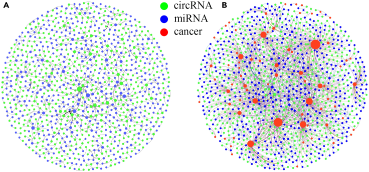
The scarcity of CMI data with experimental support is one of the challenges in the field of CMI prediction. Considering the biological property of circRNAs competitively binding miRNAs leading to cause disease, KS-CMI constructs CMCI by adding cancer as an intermediary in the CMI network to enrich the 'social relationships' of molecules in the network. The structural parameters of the CMI network and CMCI network are shown in below table.

The information on the CMI network and CMCI network

dataset	pairs	circRNA	miRNA	disease	Average degree
CMI	753	515	477	non	1.5273
CCA	648	515	Non	72	2.2003
MCA	731	non	477	72	2.6437

In addition, we visualize the CMI network and CMCI network as in figure below. Figure below shows that cancer as an intermediary molecule can effectively connect the CMI network and increase the "social relationship" of the molecule in the network, thus improving the effectiveness of the molecule's features in the network.

CMI Network and CMCI Network (each line in the figure represents a pair of relationships, and the node size is proportional to the degree.)

(A) CMI Network and (B) CMCI Network.

Molecular functional similarity construction

In the construction of molecular functional similarity, we introduce an important concept in graph theory, 'degree' (the number of edges connected to a particular node) as a measure of molecular functional similarity. Specifically, we consider that two molecules have similar functional structures if they have the same degree; if the adjacent nodes of these two molecules also have the same degree, the functional structures of these two molecules are more similar. It is worth noting that the functional similarity of molecules only focuses on whether the molecules have similar functional structures, and does not consider where the molecules are located in the network, and whether the neighboring nodes are the same.

In this work, we introduced the struc2vec⁴⁰ algorithm to extract the functional similarity features of molecules.

For nodes m and n, struc2vec first defines a structural distance D between n and m that is no greater than d:

$$D_d\left(m,n\right)=D_{d-1}\left(m,n\right)+J\left(S\left(R_d\left(m\right)\right),S\left(R_d\left(n\right)\right)\right),d\ge 0,\left|R_d\left(\right)>0\right|$$ (Equation 4)

where R_d(m) denotes the set of vertices at distance d from node m, and J() is a function measuring the distance of the ordered degree sequence, and after combining Dynamic Time Warping (DTW) optimization, J can be expressed as:

$$j\left(m,n\right)=\frac{\max \left(m,n\right)}{\min \left(m,n\right)}-1$$ (Equation 5)

Based on the structural distance D, we construct a weighted graph G with a hierarchical structure for node walk sampling. Graph G connects the same vertex of different layers (k) with weighted directed edges, and the edge weight w is defined as:

$$w\left(m_k,m_{k+1}\right)=\log \left(t_k\left(m\right)+e\right)$$ (Equation 6)

Where t_k() is the sum of the number of edges in layer k with the edge weight connected to m greater than the average edge weight.

Struc2vec samples in graph G through the biased random walk. The probability of walking from vertex m to vertex n in layer k is:

$$P\left(m,n\right)=\frac{e^{-D_k\left(m,n\right)}}{N_k\left(m\right)}$$ (Equation 7)

Where N_k() is calculated as:

$$N_k\left(m\right)={\sum }_{n\in N,n\ne m}{e}^{-D_k\left(m,n\right)}$$ (Equation 8)

The probability of sampling different layers is:

$$\begin{array}{l}{P}_k\left(m_k,m_{k+1}\right)=\frac{w\left(m_k,m_{k+1}\right)}{w\left(m_k,m_{k+1}\right)+w\left(m_k,m_{k-1}\right)}\\ P_k\left(m_k,m_{k-1}\right)=1-\frac{w\left(m_k,m_{k+1}\right)}{w\left(m_k,m_{k+1}\right)+w\left(m_k,m_{k-1}\right)}\end{array}$$ (Equation 9)

Through this walking method, struc2vec ensures that the local topological structure similarity of sampling nodes is maximized, without paying attention to the position of nodes in the graph.

Molecular Gaussian interaction profile kernel construction

The Gaussian interaction profile kernel is based on the assumption that molecules with similar targets may have the same functions, often as a useful complement to molecular features.

In the CMI-753 dataset, we constructed a c $\times$ m binary graph X_cm to store the associations, and when circRNA c_i correlates with miRNA m_j, X_ij is set to 1 and vice versa to 0. For matrix X, the Gaussian interaction profile kernel of circRNA X(c_i) and X(c_j) can be calculated as follows:

$$G\left(c_i,c_j\right)=\exp \left(-x_c{\Vert X\left(c_i\right)-X\left(c_j\right)\Vert }^2\right)$$ (Equation 10)

Where x_c controls the kernel bandwidth and is defined as:

$$x_c=1/\left(\frac{1}{nc}\sum _{i=1}^{nc}{\Vert X\left(c_i\right)\Vert }^2\right)$$ (Equation 11)

Similarly, the GIPK of miRNA X(m_i) and X(m_j) is defined as

$$G\left(m_i,m_j\right)=\exp \left(-x_m{\Vert X\left(m_i\right)-X\left(m_j\right)\Vert }^2\right)$$ (Equation 12)

$$x_m=1/\left(\frac{1}{nm}\sum _{i=1}^{nm}{\Vert X\left(m_i\right)\Vert }^2\right)$$ (Equation 13)

Denoising autoencoder

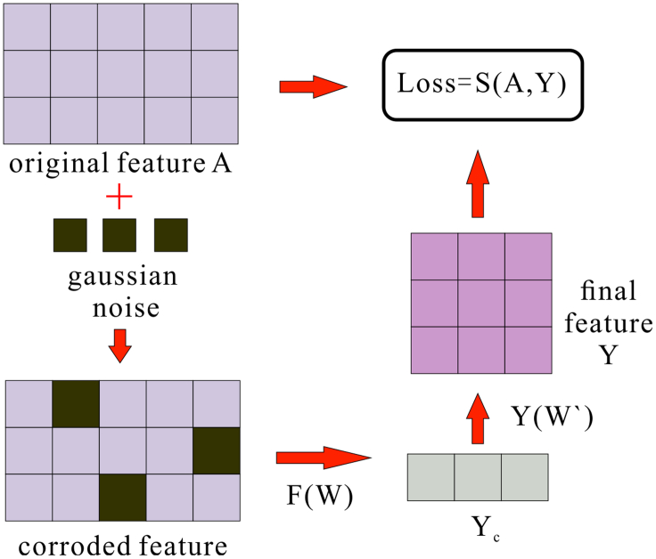
KS-CMI uses DAE³³ to simulate human thinking mode to learn the robust representation of molecular features. In short, DAE forces the neural network to learn the high-level representation of the original features from the original features after corrosion, and the features obtained are not only of lower dimensions but also more representative. The flowchart of DAE is shown in below figure. First, the DAE obtains the corroded feature $\tilde{A}$ by adding Gaussian noise to the original input feature A. The project $\tilde{A}$ into a new hidden representation Y_c through the function F.

The flowchart of DAE

$$Y_c=q_{a,\lambda }\left(\tilde{A}\right)=F\left(W·\tilde{A}+b\right)$$ (Equation 14)

Similarly, the reconstruct uncorroded features Y as:

$$Y=q_{b,\beta }\left(A\right)=F\left(W^{\prime }·A+b^{\prime }\right)$$ (Equation 15)

The function F can be represented as:

$$F\left(x\right)=\frac{1}{\left(1+e^{-x}\right)}$$ (Equation 16)

Then DAE continuously optimizes parameters (q_a,λ, q_b,β) by minimizing the average reconstruction error

$${\lambda }^o,{\beta }^o=\underset{\lambda \beta }{\mathrm{argmin}}\frac{1}{j}\sum _{i=1}^{j}S\left(A^{\left(m\right)},t^{\left(m\right)}\right)=\underset{\lambda \beta }{\mathrm{argmin}}\frac{1}{j}\sum _{i=1}^{j}S\left(A^{\left(m\right)},q_{b,\beta }\left(q_{a,\lambda }\left({\tilde{A}}^{\left(m\right)}\right)\right)\right)$$ (Equation 17)

Where j is the number of train data, λ⁰, β⁰ is the optimal values of λ, β. S is the reconstruction error which is:

$$S=-\frac{1}{j}\sum _{n=1}^j{y}_n·\log {\hat{y}}_n+\left(1-y_n\right)·\log \left(1-{\hat{y}}_n\right)$$ (Equation 18)

Molecular social relationship descriptors

Previous work has focused on capturing the behavior features of nodes from constructed binary networks. These methods treat known positive samples as related but ignore negative samples and the rich chain relationships in the relational network.

In this paper, we introduce the concept of social relationships in the KS-CMI and extract the social relationship representation of molecules from the CMCI network by the signed graph convolution neural network (SGCN),⁴¹ combined with the balanced path.

Social relationship building

Social relationships describe networks from the point of view of friends and foes. Similarly, we reconstructed the relational network form of the data, in which the known positive sample N⁺ in the data N is defined as 1, i.e., friend, and the negative sample N^- is defined as -1, i.e., foe.

$$N=N^{+}\cup N^{-}$$ (Equation 19)

$$N^{+}\cap N^{-}=\varnothing$$ (Equation 20)

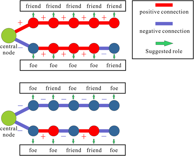
Interestingly, social relationships are not just first-order relationships. For example, friends of a friend can still be friends, and foes of a friend can be foes. Bioinformatically speaking, if molecule 1 and molecule 2 are related (i.e., the two molecules are friends) and molecule 2 is related to molecule 3, then molecule 1 and molecule 3 have similar functions or binding sites (i.e., a friend of a friend is still a friend). If molecule 1 is related to molecule 2, but molecule 2 is not related to molecule 3 (i.e., the two are foes), then molecule 1 is unrelated to molecule 3 (i.e., the enemy of a friend is still a foe). Using the balanced path approach can significantly improve the connection between molecules in a sparse network, forming a unique ‘chain association’. Such an explanation is not only scientific but also allows for the extraction of additional hidden features from social relationships. To effectively describe multi-order relationships, we defined balanced paths in conjunction with balance theory.

The balanced path is shown in below figure. Simply put, in a balanced path of L length, the path containing an even number of negative connections is considered to be balanced, i.e., friends and the path containing the odd number of negative connections are unbalanced, i.e., foes. We can recursively define a balanced path of L+1 length as follows:

$$\begin{array}{l}L>1\\ P_u\left(L+1\right)=\left\{x_u|x_k\in P_u\left(L\right)and{x}_u\in N_k^{+}\right\}\cup \left\{x_u|x_k\in G_u\left(L\right)and{x}_u\in N_k^{-}\right\}\\ G_u\left(L+1\right)=\left\{x_u|x_k\in G_u\left(L\right)and{x}_u\in N_k^{+}\right\}\cup \left\{x_u|x_k\in P_u\left(L\right)and{x}_u\in N_k^{-}\right\}\end{array}$$ (Equation 21)

Where P_u(L+1) represents the neighbor set of the balanced path from x_u and G_u(L+1) represents the neighbor set of the unbalanced path from x_u.

Balanced path of central node based on the balance theory

Social relationship extraction

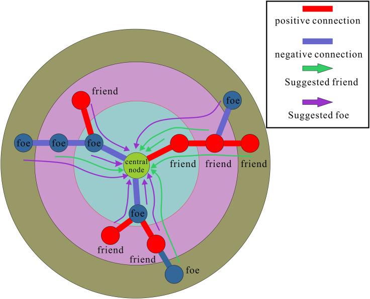
The construction of social relations is based on the graph structure data propagation of traditional graph neural networks. First, the node itself is used as the central node to aggregate the first-order neighbor information adjacent to it to obtain the feature representation of the central node, and then data propagation is performed on the graph structure by superimposing a multilayer network structure to obtain the multi-order neighbor information of the central node.

The difference is that in social networks, the neighbors of the central node have their social attributes. SGCN does not maintain a single representation of each node but integrates positive and negative link information through a balanced path that simultaneously preserves the social relationships of multiple-order neighbors. The aggregation process is shown in below figure.

The aggregation process of SGCN

For each node n in the CMCI, we initialize the eigenvectors of each node first. In KS-CMI, to demonstrate the impact of social characteristics on model ability, we used SVD-derived characteristic d as the initial feature of the node.

Next, in the social relationship graph composed of nodes with initial features, the first layer of convolutional aggregation for any central node u by w() is as follows:

$$H_i^{P\left(1\right)}=\mu \left(w^{P\left(1\right)}\left[\sum _{j\notin N_i^{+}}\frac{H_j^{\left(0\right)}}{\left|N^{+}\right|}\right],H_i^{\left(0\right)}\right)$$ (Equation 22)

$$H_i^{G\left(1\right)}=\mu \left(w^{G\left(1\right)}\left[\sum _{c\notin N_i^{-}}\frac{H_c^{\left(0\right)}}{\left|N^{-}\right|}\right],H_i^{\left(0\right)}\right)$$ (Equation 23)

Where ${\mathrm{H}}_{\mathrm{i}}^{\left(0\right)}$ is the initial features of u, H^P(1) and H^G(1) is the friend feature representation and foe feature representation of u respectively, and μ() is the activation function.

As the number of aggregation layers in the model increases, when layer l>1, the aggregation function is recursively defined as:

$$\begin{array}{l}l>1\\ H_i^{P\left(l\right)}=\mu \left(w^{P\left(l\right)}\left[\sum _{j\notin N_i^{+}}\frac{H_j^{P\left(l-1\right)}}{\left|N_i^{+}\right|},\sum _{c\notin N_i^{-}}\frac{H_c^{G\left(l-1\right)}}{\left|N_i^{-}\right|},H_i^{P\left(l-1\right)}\right]\right)\\ H_i^{G\left(l\right)}=\mu \left(w^{G\left(l\right)}\left[\sum _{j\notin N_i^{+}}\frac{H_j^{G\left(l-1\right)}}{\left|N_i^{+}\right|},\sum _{c\notin N_i^{-}}\frac{H_c^{P\left(l-1\right)}}{\left|N_i^{-}\right|},H_i^{G\left(l-1\right)}\right]\right)\end{array}$$ (Equation 24)

After L iterations of computation, the friend representation and foe representation of the central node u are updated to ${\mathrm{H}}_{\mathrm{i}}^{\mathrm{P}\left(\mathrm{l}\right)}$, ${\mathrm{H}}_{\mathrm{i}}^{\mathrm{G}\left(\mathrm{l}\right)}$.

Next, two feature representations of the learned central node u are connected as a single feature representation.

To make the node feature fully represent the multi-order social relation of the node, we use the objective function F to optimize and obtain the final feature representation. Target function F is defined as:

$$F\left({\beta }^w,{\beta }^{MLG}\right)=-\frac{1}{S}\sum _{\left(u_i,u_j,r\right)\in S}{\alpha }_r\log \frac{\exp \left(\left[z_i,z_j\right]{\beta }_r^{MLG}\right)}{\sum _{q\in \left\{+,-,?\right\}}\exp \left(\left[z_i,z_j\right]{\beta }_q^{MLG}\right)}+\delta [\frac{1}{\left|S_{\left(+,?\right)}\right|}\sum _{\left(\left(u_i,u_j,u_k\right)\in S_{\left(+,?\right)}\right)}\max \left(0,\left(\Vert z_i-z_j|{|}_2^2-\Vert z_i-z_k|{|}_2^2\right)\right)+\frac{1}{\left|S_{\left(-,?\right)}\right|}\sum _{\left(\left(u_i,u_j,u_k\right)\in S_{\left(-,?\right)}\right)}\max \left(0,\left(\Vert z_i-z_k|{|}_2^2-\Vert z_i-z_j|{|}_2^2\right)\right)]+\mathrm{R}\mathrm{e}g\left({\beta }^w,{\beta }^{MLG}\right)$$ (Equation 25)

Function F() uses the relationship between nodes and balance theory to learn the characteristics of nodes. For the relationship between nodes, the model uses the MLG classifier to classify nodes and judge the relationship type r between nodes. Moreover, in the representation of balance theory in space, if two nodes have a friend relationship, they should be closer than those without, and vice versa.

In the function F(), β^w is the parameter of the convolution layer aggregation function, β^MLG is the parameter of the MLG classifier, and α_r is the weight of the type of connection between nodes. S_(+,?) and S_(-,?) represent node pairs with friend/foe relationships, respectively (u_i, u_j), u_k represents the nodes that are not related to either u_i, or u_j , REG is the regularization of a function F().

Finally, by optimizing the target function, we get a single 64-dimensional representation of the social relationships of each node in the social network.

Classification strategy

Catboost³⁴ (categorical boosting) is an improved classifier based on the GBDT algorithm framework. It adopts oblivious trees as a learner and resolves gradient bias and prediction shift in traditional algorithms so that Catboost has good accuracy and generalization. Catboost has a unique advantage in dealing with multi-data types and categorical features.

KS-CMI uses Catboost as a model classification strategy. Specifically, the attribute descriptors and social descriptors of the samples in the training set were connected and sent to the Catboost classifier to learn the labeling attributes of the sample. The trained classifier then predicted the labeling attributes in the test set and scored them.

In this work, we select the optimal parameters for the final prediction task by the grid search method.

Quantification and statistical analysis

The ROC and PR curve plotting, area under the curve calculation, and evaluation criteria calculation were performed using Scikit-learn 0.24.2.

Published: July 26, 2023

Data and code availability

• •Data reported in this paper will be shared by the lead contact upon request. This paper analyzes existing, publicly available data. These accession numbers for the datasets are listed in the key resources table.
• •This paper does not report original code.
• •Any additional information required to reanalyze the data reported in this paper is available from the lead contact upon request.

References

- 1.Jeck W.R., Sharpless N.E. Detecting and characterizing circular RNAs. Nat. Biotechnol. 2014;32:453–461. doi: 10.1038/nbt.2890. [DOI] [PMC free article] [PubMed] [Google Scholar]
- 2.Haque S., Harries L.W. Circular RNAs (circRNAs) in health and disease. Genes. 2017;8:353. doi: 10.3390/genes8120353. [DOI] [PMC free article] [PubMed] [Google Scholar]
- 3.Sanger H.L., Klotz G., Riesner D., Gross H.J., Kleinschmidt A.K. Viroids are single-stranded covalently closed circular RNA molecules existing as highly base-paired rod-like structures. Proc. Natl. Acad. Sci. USA. 1976;73:3852–3856. doi: 10.1073/pnas.73.11.3852. [DOI] [PMC free article] [PubMed] [Google Scholar]
- 4.Armakola M., Higgins M.J., Figley M.D., Barmada S.J., Scarborough E.A., Diaz Z., Fang X., Shorter J., Krogan N.J., Finkbeiner S., et al. Inhibition of RNA lariat debranching enzyme suppresses TDP-43 toxicity in ALS disease models. Nat. Genet. 2012;44:1302–1309. doi: 10.1038/ng.2434. [DOI] [PMC free article] [PubMed] [Google Scholar]
- 5.Wei J., Wei W., Xu H., Wang Z., Gao W., Wang T., Zheng Q., Shu Y., De W. Circular RNA hsa_circRNA_102958 may serve as a diagnostic marker for gastric cancer. Cancer Biomarkers. 2020;27:139–145. doi: 10.3233/CBM-182029. [DOI] [PubMed] [Google Scholar]
- 6.Zhao S.-Y., Wang J., Ouyang S.-B., Huang Z.-K., Liao L., Biochemistry Salivary circular RNAs Hsa_Circ_0001874 and Hsa_Circ_0001971 as novel biomarkers for the diagnosis of oral squamous cell carcinoma. Cell. Physiol. Biochem. 2018;47:2511–2521. doi: 10.1159/000491624. [DOI] [PubMed] [Google Scholar]
- 7.He Y.-D., Tao W., He T., Wang B.-Y., Tang X.-M., Zhang L.-M., Wu Z.-Q., Deng W.-M., Zhang L.-X., Shao C.K., et al. A urine extracellular vesicle circRNA classifier for detection of high-grade prostate cancer in patients with prostate-specific antigen 2–10 ng/mL at initial biopsy. Mol. Cancer. 2021;20:96. doi: 10.1186/s12943-021-01388-6. [DOI] [PMC free article] [PubMed] [Google Scholar]
- 8.Chen X., Xie D., Zhao Q., You Z.-H. MicroRNAs and complex diseases: from experimental results to computational models. Briefings Bioinf. 2019;20:515–539. doi: 10.1093/bib/bbx130. [DOI] [PubMed] [Google Scholar]
- 9.Chen X., Yan C.C., Zhang X., You Z.-H., Deng L., Liu Y., Zhang Y., Dai Q. WBSMDA: within and between score for MiRNA-disease association prediction. Sci. Rep. 2016;6:21106–21109. doi: 10.1038/srep21106. [DOI] [PMC free article] [PubMed] [Google Scholar]
- 10.You Z.-H., Huang Z.-A., Zhu Z., Yan G.-Y., Li Z.-W., Wen Z., Chen X.J.P.c.b. Vol. 13. 2017. (PBMDA: A Novel and Effective Path-Based Computational Model for miRNA-Disease Association Prediction). [DOI] [PMC free article] [PubMed] [Google Scholar]
- 11.Lei X., Mudiyanselage T.B., Zhang Y., Bian C., Lan W., Yu N., Pan Y. A comprehensive survey on computational methods of non-coding RNA and disease association prediction. Briefings Bioinf. 2021;22 doi: 10.1093/bib/bbaa350. [DOI] [PubMed] [Google Scholar]
- 12.Zhang Y., Lei X., Pan Y., Pedrycz W. Prediction of disease-associated circRNAs via circRNA–disease pair graph and weighted nuclear norm minimization. Knowl. Base Syst. 2021;214 doi: 10.1016/j.knosys.2020.106694. [DOI] [Google Scholar]
- 13.Wang L., You Z.-H., Huang Y.-A., Huang D.-S., Chan K.C.C. An efficient approach based on multi-sources information to predict circRNA–disease associations using deep convolutional neural network. Bioinformatics. 2020;36:4038–4046. doi: 10.1093/bioinformatics/btz825. [DOI] [PubMed] [Google Scholar]
- 14.Guo Y., Lei X., Liu L., Pan Y. circ2CBA: prediction of circRNA-RBP binding sites combining deep learning and attention mechanism. Front. Comput. Sci. 2022;17 doi: 10.1007/s11704-022-2151-0. [DOI] [Google Scholar]
- 15.Wang Z., Lei X. Prediction of RBP binding sites on circRNAs using an LSTM-based deep sequence learning architecture. Briefings Bioinf. 2021;22:bbab342. doi: 10.1093/bib/bbab342. [DOI] [PubMed] [Google Scholar]
- 16.Yang J., Lei X. Predicting circRNA-disease associations based on autoencoder and graph embedding. Inf. Sci. 2021;571:323–336. doi: 10.1016/j.ins.2021.04.073. [DOI] [Google Scholar]
- 17.Fan C., Lei X., Tie J., Zhang Y., Wu F.-X., Pan Y. CircR2Disease v2.0: An Updated Web Server for Experimentally Validated circRNA–disease Associations and Its Application. Dev. Reprod. Biol. 2022;20:435–445. doi: 10.1016/j.gpb.2021.10.002. [DOI] [PMC free article] [PubMed] [Google Scholar]
- 18.Liu M., Wang Q., Shen J., Yang B.B., Ding X. Circbank: a comprehensive database for circRNA with standard nomenclature. RNA Biol. 2019;16:899–905. doi: 10.1080/15476286.2019.1600395. [DOI] [PMC free article] [PubMed] [Google Scholar]
- 19.Fan, C., Lei, X., Fang, Z., Jiang, Q., and Wu, F.-X.J.D. (2018). CircR2Disease: A Manually Curated Database for Experimentally Supported Circular RNAs Associated with Various Diseases. 2018. [DOI] [PMC free article] [PubMed]
- 20.Glažar P., Papavasileiou P., Rajewsky N.J.R. circBase: a database for circular RNAs. RNA. 2014;20:1666–1670. doi: 10.1261/rna.043687.113. [DOI] [PMC free article] [PubMed] [Google Scholar]
- 21.Liu M., Wang Q., Shen J., Yang B.B., Ding X.J.R.b. Vol. 16. 2019. pp. 899–905. (Circbank: A Comprehensive Database for circRNA with Standard Nomenclature). [DOI] [PMC free article] [PubMed] [Google Scholar]
- 22.Guo L.X., You Z.H., Wang L., Yu C.Q., Zhao B.W., Ren Z.H., Pan J. A novel circRNA-miRNA association prediction model based on structural deep neural network embedding. Briefings Bioinf. 2022;23 doi: 10.1093/bib/bbac391. [DOI] [PubMed] [Google Scholar]
- 23.Qian Y., Zheng J., Jiang Y., Li S., Deng L. Prediction of circRNA-miRNA Association Using Singular Value Decomposition and Graph Neural Networks. IEEE/ACM Trans Comput Biol Bioinform. 2022 doi: 10.1109/TCBB.2022.3222777. [DOI] [PubMed] [Google Scholar]
- 24.He J., Xiao P., Chen C., Zhu Z., Zhang J., Deng L. GCNCMI: A Graph Convolutional Neural Network Approach for Predicting circRNA-miRNA Interactions. Front. Genet. 2022;13 doi: 10.3389/fgene.2022.959701. [DOI] [PMC free article] [PubMed] [Google Scholar]
- 25.Wang X.-F., Yu C.-Q., Li L.-P., You Z.-H., Huang W.-Z., Li Y.-C., Ren Z.-H., Guan Y.-J. KGDCMI: A New Approach for Predicting circRNA–miRNA Interactions from Multi-Source Information Extraction and Deep Learning. Front Genet. 2022;13 doi: 10.3389/fgene.2022.958096. [DOI] [PMC free article] [PubMed] [Google Scholar]
- 26.Yu C.Q., Wang X.F., Li L.P., You Z.H., Huang W.Z., Li Y.C., Ren Z.H., Guan Y.J. SGCNCMI: A New Model Combining Multi-Modal Information to Predict circRNA-Related miRNAs, Diseases and Genes. Biology. 2022;11:1350. doi: 10.3390/biology11091350. [DOI] [PMC free article] [PubMed] [Google Scholar]
- 27.Wang X.-F., Yu C.-Q., You Z.-H., Li L.-P., Huang W.-Z., Ren Z.-H., Li Y.-C., Wei M.-M. A feature extraction method based on noise reduction for circRNA-miRNA interaction prediction combining multi-structure features in the association networks. Briefings Bioinf. 2023;24:bbad111. doi: 10.1093/bib/bbad111. [DOI] [PubMed] [Google Scholar]
- 28.Enright A.J., John B., Gaul U., Tuschl T., Sander C., Marks D.S. Genome Biol. 2003;5:1–27. doi: 10.1186/gb-2003-5-1-r1. [DOI] [PMC free article] [PubMed] [Google Scholar]
- 29.Lewis B.P., Shih I.-h., Jones-Rhoades M.W., Bartel D.P., Burge C.B. Prediction of mammalian microRNA targets. Prediction of mammalian microRNA targets. 2003;115:787–798. doi: 10.1016/s0092-8674(03)01018-3. [DOI] [PubMed] [Google Scholar]
- 30.Lan, W., Zhu, M., Chen, Q., Chen, B., Liu, J., Li, M., and Chen, Y.-P.P.J.D. (2020). CircR2Cancer: A Manually Curated Database of Associations between circRNAs and Cancers. 2020. [DOI] [PMC free article] [PubMed]
- 31.Lan, W., Zhu, M., Chen, Q., Chen, J., Ye, J., Liu, J., Peng, W., and Pan, S.J.C. (2021). Prediction of circRNA-miRNA Associations Based on Network Embedding. 2021.
- 32.Yao D., Nong L., Qin M., Wu S., Yao S. Identifying circRNA-miRNA interaction based on multi-biological interaction fusion. Front. Microbiol. 2022;13:987930. doi: 10.3389/fmicb.2022.987930. [DOI] [PMC free article] [PubMed] [Google Scholar]
- 33.Vincent, P., Larochelle, H., Bengio, Y., and Manzagol, P.-A. (2008). Extracting and Composing Robust Features with Denoising Autoencoders. pp. 1096-1103.
- 34.Dorogush, A.V., Ershov, V., and Gulin, A.J.a.p.a. (2018). CatBoost: gradient boosting with categorical features support.
- 35.Breiman L. Mach. Learn. 2001;45:5–32. [Google Scholar]
- 36.LaValley M.P. Logistic regression. Circulation. 2008;117:2395–2399. doi: 10.1161/CIRCULATIONAHA.106.682658. [DOI] [PubMed] [Google Scholar]
- 37.Guo G., Wang H., Bell D., Bi Y., Greer K. Springer; 2003. KNN Model-Based Approach in Classification; pp. 986–996. [Google Scholar]
- 38.Wang H., Hao F. IEEE; 2012. An Efficient Linear Regression Classifier; pp. 1–6. [Google Scholar]
- 39.Qian Y., Zheng J., Jiang Y., Li S., Deng L. Prediction of circRNA-miRNA Association using Singular Value Decomposition and Graph Neural Networks. IEEE ACM Trans. Comput. Biol. Bioinf. 2022:1–9. doi: 10.1109/TCBB.2022.3222777. [DOI] [PubMed] [Google Scholar]
- 40.Ribeiro, L.F., Saverese, P.H., and Figueiredo, D.R. (2017). struc2vec: Learning Node Representations from Structural Identity. pp. 385-394.
- 41.Derr T., Ma Y., Tang J. IEEE; 2018. Signed Graph Convolutional Networks; pp. 929–934. [Google Scholar]
Associated Data
This section collects any data citations, data availability statements, or supplementary materials included in this article.
Data Availability Statement