Meta-analysis of Diagnostic Test Accuracy Assessment Studies with Varying Number of Thresholds

Summary.

Current meta-analytic methods for diagnostic test accuracy are generally applicable to a selection of studies reporting only estimates of sensitivity and specificity, or at most, to studies whose results are reported using an equal number of ordered categories. In this article, we propose a new meta-analytic method to evaluate test accuracy and arrive at a summary receiver operating characteristic (ROC) curve for a collection of studies evaluating diagnostic tests, even when test results are reported in an unequal number of nonnested ordered categories. We discuss both non-Bayesian and Bayesian formulations of the approach. In the Bayesian setting, we propose several ways to construct summary ROC curves and their credible bands. We illustrate our approach with data from a recently published meta-analysis evaluating a single serum progesterone test for diagnosing pregnancy failure.

1. Introduction

The need for comprehensive evaluation of diagnostic tests is motivated by clinical, as well as health policy-making, considerations (Irwig et al., 1994). From the clinical standpoint, proper assessment of test accuracy facilitates the correct use and interpretation of test results. From the health policy-making point of view, test accuracy assessment provides a basis for a cost-benefit evaluation of the test and its performance vis-à-vis alternative testing procedures. Given these considerations, a systematic review and synthesis of all published information about a diagnostic test are necessary for the overall assessment of its diagnostic value.

Statistical methodology for meta-analysis of diagnostic accuracy studies has largely been focused on the most common type of studies—those reporting estimates of test sensitivity and specificity. Meta-analytic models have been developed to combine information from such studies in both fixed and random-effect frameworks (Moses, Shapiro, and Littenberg, 1993; Irwig et al., 1994; Hasselblad and Hodges, 1995; Irwig et al., 1995; Shapiro, 1995; Rutter and Gatsonis, 1995, 2001; Hellmich, Abrams, and Sutton, 1999; Kester and Buntinx, 2000). However, for studies where test results are reported in a potentially unequal number of categories, no standard method has been devised. In some instances, outcome categories are collapsed into two groups, and only one pair of specificity and sensitivity per study is used in the analysis. Alternatively, as shown in Mol et al. (1998), weighted combinations of all pairs of categories from the same study may be used. In meta-analysis of treatment effects, Dominici et al. (1999) suggest a latent variable method to convert continuous and dichotomous treatment outcomes to a common continuous scale. Similarly, Whitehead et al. (2001) develop fixed and random-effects models to combine ordinal outcomes from treatment effect studies.

In this article, we present a new method for meta-analysis of diagnostic test studies that can be used to synthesize results from studies where test outcomes are reported in an unequal number of nonnested ordered categories. After an overview of ROC analysis and summary ROC curves in Section 2, in Section 3, we introduce the fixed-effects meta-analysis model and discuss the construction of summary ROC curves and their confidence bands. Section 4 introduces the hierarchical formulation of the meta-analytic model, with several suggested methods for summarizing diagnostic test accuracy and assessing its variability. In Section 5 we present an application of the methodologies from Sections 3 and 4 to the pregnancy failure data of Mol et al. (1998), concluding with a discussion in Section 6.

2. ROC Analysis and Summary ROC Curves

Diagnostic accuracy of a test refers to its ability to correctly diagnose the true disease status. To assess the accuracy, test results have to be compared against the truth (or the “gold standard”), ascertained usually via more costly and complex procedures, such as biopsy or surgery. The fraction of patients found to be correctly diagnosed as positive (true positive rate, or sensitivity), and those correctly diagnosed as negative (true negative rate, or specificity) are two typical measures of diagnostic accuracy. It is important to note that both sensitivity and specificity are tied to the particular underlying diagnostic threshold that defines test outcomes as “positive” (T⁺) or “negative” (T⁻ ). A perhaps better measure of test accuracy is the receiver operating characteristic (ROC) curve (Swets and Pickett, 1982). The ROC curve is a plot of all pairs of true positive and false positive rates, found as the diagnostic threshold ranges over all possible values.

The ROC curve provides a detailed portrait of test accuracy. In practice, several low-dimensional functionals are used to summarize and compare ROC curves. One of the most common summary measures is area under the curve (AUC). It takes values between 0 and 1, and can be interpreted as $Pr\left(Y_1>Y_2\right)$, the probability that in a randomly chosen pair of a diseased and a nondiseased case, the diseased case is correctly ranked as more likely to have the disease. The nonparametric AUC estimator is in fact the Mann-Whitney version of the Wilcoxon two-sample rank sum statistic (Bamber, 1975; Hanley, 1998). The values of AUC that are closer to 1 indicate more accurate tests, while a test with AUC below 0.5 is worse than a coin flip in assigning diagnoses to patients.

Other functionals, such as the partial area and the $Q^{*}$ statistic are also used. The partial area (PAUC) is AUC evaluated over a subrange of threshold values whose sensitivity and specificity are clinically relevant (McClish, 1989). The $Q^{*}$ statistic (Moses et al., 1993) is defined as the point on the ROC curve where sensitivity equals specificity. In cases where ROC curves are symmetric or nearly symmetric, the $Q^{*}$ statistic can be used to compare tests in terms of diagnostic accuracy. Larger $Q^{*}$ values correspond to ROC curves shouldering up more closely to the desirable corner where both specificity and sensitivity are high.

2.1. Estimation of ROC Curves

The empirical ROC curve is a square-grid plot of (sensitivity, 1-specificity) pairs, estimated at each reported diagnostic threshold. A smooth ROC curve can be estimated via parametric methods (McCullagh, 1980; Tosteson and Begg, 1988; Pepe, 2000) or semi- and nonparametric methods (Zou, Hall, and Shapiro, 1997; Pepe, 2000).

Parametric ROC analysis for ordinal categorical test results has a close link to ordinal regression. To illustrate, consider a study where a single test is administered and the results are reported using $J-1$ thresholds, that is, in $J$ ordered categories. Let $Y_i$ denote the test result of the $i$-th patient, where $Y_i\in \{1,\dots ,J\}$. For example, a 5-category scale is often used in the evaluation of diagnostic imaging, ranging from 1 = “definitely normal” to 5 = “definitely abnormal.” We assume that each response $Y_i$ arises from an underlying latent continuous variable $M_i$ via discretization at thresholds ${\theta }_0<\cdots {\theta }_j\cdots <{\theta }_J$, so that $Y_i=j$ when ${\theta }_{j-1}<M_i<{\theta }_j$, where ${\theta }_0=-\infty$ and ${\theta }_J=\infty$. Let $D_i$ indicate the true disease status of the patient $i$ with $D_i=1$ if disease is present and $D_i=0$ if not. Then, the simplest ordinal regression model with only one covariate (disease status) is given as follows:

$$g\left\{P\left(Y_i\le j\mid D_i\right)\right\}=\frac{{\theta }_j-\beta D_i}{\text{exp}\left(\alpha D_i\right)}.$$ (1)

The link $g$ is a monotone function such that $0\le g^{-1}(\cdot )\le 1$, often probit or logit. Given $\alpha$ and $\beta$, formula (1) yields false positive $\left(P\left(T^{+}\mid D^{-}\right)=P\left(M_i\le \theta \mid D_i=0\right)\right)$ and true positive rates $\left(P\left(T^{+}\mid D^{+}\right)=P\left(M_i\le \theta \mid D_i=1\right)\right)$ for any threshold $\theta$, resulting in a continuous ROC curve. $\beta$ is commonly referred to as the location and $\alpha$ as the scale of the ROC curve.

Other covariates besides $D_i$ can easily be incorporated into (1). For example,

$$g\left\{P\left(Y_i\le j\mid D_i,{\mathbf{X}}_i^{\left(l\right)},{\mathbf{X}}_i^{\left(s\right)}\right)\right\}=\frac{{\theta }_j-\beta D_i+\delta {\mathbf{X}}_i^{\left(l\right)}}{\text{exp}\left(\alpha D_i+\gamma {\mathbf{X}}_i^{\left(s\right)}\right)}.$$ (2)

Here, ${\mathbf{X}}_i^{\left(l\right)}$ and ${\mathbf{X}}_i^{\left(s\right)}$ are the patient i’s vectors of location and scale covariates, of dimensions $q_l$ and $q_s$, respectively, possibly including interactions between covariates or interactions between covariates and disease status. Inclusion of covariates results in a model that yields a separate ROC curve for each unique combination of covariate levels. Note that when the test results are binary, a trivial empirical ROC curve is obtained, with only one observed pair of sensitivity and specificity estimates. In such situations, the full ROC model (1) cannot be estimated without specifying one of the unknown parameters, $\alpha$ or $\beta$; often, $\alpha$ is fixed at 0 and a symmetric ROC curve is obtained.

2.2. Summary ROC Curves

One of the main goals of a meta-analysis of diagnostic accuracy studies is to provide a summary measure of diagnostic accuracy based on a collection of studies and their reported empirical or estimated smooth ROC curves. When all involved studies use a dichotomous reporting scheme (reporting sensitivity and specificity estimates only), the simplest summary measure would be the average sensitivity and specificity. However, this would be valid only if it were known that all studies used the same diagnostic threshold.

Moses et al. (1993) have proposed a method that accounts for threshold differences, by essentially fitting a summary ROC (SROC) curve to the scatterplot of all sensitivity and specificity pairs from studies with two categories. Their SROC curve is constructed by calculating two quantities: ${ℬ}_k=\text{logit}\left({\widehat{\text{TPR}}}_k\right)-\text{logit}\left({\widehat{\text{FPR}}}_k\right)$ and ${𝒮}_k=$ $\text{logit}\left({\widehat{\text{TPR}}}_k\right)+\text{logit}\left({\widehat{\text{FPR}}}_k\right)$, where $\text{logit}\left(p\right)=\text{ln}(p/(1-p\left)\right)$ and ${\widehat{\text{TPR}}}_k$ and ${\widehat{\text{FPR}}}_k$ represent the reported sensitivity and 1-specificity for study $k$. The estimates ${\widehat{\lambda }}_0$ and ${\widehat{\lambda }}_1$ from the model ${ℬ}_k={\lambda }_0+{\lambda }_1{𝒮}_k+e_k$ are then used to estimate the “summary” relation between FPR (false positive rate) and TPR (true positive rate), yielding a smooth SROC curve. This SROC model can be extended to include study-level covariates. A binary regression approach to the problem of combining data from studies reporting pairs of sensitivity and specificity has also been proposed by Rutter and Gatsonis (1995, 2001).

To meta-analyze studies with results in more than two categories, one approach is to dichotomize results by grouping them into two categories and then employing the above method. However, it is more efficient to take all thresholds into account. Some work has been published on methodology that could be used in meta-analysis of ROC studies with equal number of aligned categories (Gatsonis, 1995; Ishwaran and Gatsonis, 2000). None of these approaches, however, is able to accommodate meta-analyses with test results reported in an unequal number of (nonaligned) categories.

In this article, we consider both a fixed-effects and a random-effects formulation of meta-analysis of studies with an unequal number of nonnested categories. The random-effects formulation employs a hierarchical ordinal regression model, which allows for heterogeneity of studies beyond what could be contributed to different thresholds, and accounts for within-study correlation. This approach relaxes the assumption that all studies have the same underlying ROC curve; rather, it assumes that each study estimates a study-specific ROC curve that can be viewed as a random sample from a population of all ROC curves of such studies.

3. Fixed-Effects Meta-analysis Model

The fixed-effects framework for meta-analysis usually focuses on estimating a single summary measure of interest based on the information provided in the individual studies (Cooper and Hedges, 1994). The salient feature of the fixed-effects model is that it contains no between-study component of variation. Our fixed-effects model for meta-analysis of test accuracy studies is based on the assumption that all studies have the same scale and location parameters, and hence the common ROC curve. However, the model assumes that each study has its own set of thresholds, $\mathit{\theta }$, independent from the thresholds used in other studies. Thus, the observed differences are thought to result only from different diagnostic thresholds.

Let $\mathbf{\Theta }=(\mathit{\theta },\alpha ,\beta ,\gamma ,\mathit{\delta })$ be the vector containing thresholds from every study, location and scale parameters, and regression coefficients. Denote by $Y_{ik}$ the observed test outcome for the $i$th patient from the $k$th study. Assume for now that we only have disease status $D_{ik}$ as a covariate. Then, the likelihood based on the data from $K$ studies is given as follows:

$$\begin{gathered} L(\mathbf{\Theta }\mid \mathbf{Y})= \prod _{k=1}^K \prod _{j=1}^{J_k} \prod _{i\in G_{jk}} \left[g^{-1}\left(\frac{\left({\theta }_{j,k}-\beta D_{i,k}\right)}{\text{exp}\left(\alpha D_{i,k}\right)}\right)\right. \\ {\left.-g^{-1}\left(\frac{{\theta }_{j-1,k}-\beta D_{i,k}}{\text{exp}\left(\alpha D_{i,k}\right)}\right)\right]}^{I\left(y_{ik}=j\right)} \end{gathered}$$ (3)

where $G_{jk}$ is the group of patients from study $k$ whose test outcomes fall into $j$th category, $g^{-1}\left(\left({\theta }_{j,k}-\beta D_{i,k}\right)/\mathrm{e}\mathrm{x}\mathrm{p}\left(\alpha D_{i,k}\right)\right)$ is assumed to be 1 when $j=J_k$ and 0 when $j=0;I(\cdot )$ is the indicator function. Estimation of parameters can be done via numerical maximization of the likelihood (3). The program was written in Matlab 5.3 and can be obtained on request. The SROC curve is then obtained by plotting the pairs $(\widehat{\mathrm{T}\mathrm{P}\mathrm{R}},\widehat{\mathrm{F}\mathrm{P}\mathrm{R}})$ at each threshold :

$$\begin{gathered} \widehat{\mathrm{T}\mathrm{P}\mathrm{R}}\left(\theta \right) =P\left(T^{+}\mid D^{+},\theta \right)=P(Y\le \theta \mid D=1) \\ =g^{-1}\left(\frac{\left(\theta -\widehat{\beta }{D}_{i,k}\right)}{\mathrm{e}\mathrm{x}\mathrm{p}\left(\widehat{\alpha }{D}_{i,k}\right)}\right) \\ \widehat{\mathrm{F}\mathrm{P}\mathrm{R}}\left(\theta \right) =P\left(T^{+}\mid D^{-},\theta \right)=P(Y\le \theta \mid D=0)=g^{-1}\left(\theta \right), \end{gathered}$$

where $\widehat{\alpha }$ and $\widehat{\beta }$ correspond to the maximum likelihood estimates of the scale and location, respectively. If additional covariates are present in the model in such a way that they affect test accuracy (either through interacting with disease status or directly affecting the scale), an SROC curve is defined separately for each unique combination of levels of these covariates.

The SROC curve summarizes the overall performance of a diagnostic test, and on the basis of it, one can compare one test to another. To do this, we need to assess the variability of the estimated SROC curve. The variance of every point on the estimated SROC curve can be obtained either by the delta method or by bootstrap. The latter adjusts the intervals for the correlation of outcomes within the studies. The variance estimates can then be used to derive the upper and lower pointwise confidence bands around the estimated SROC curve.

4. Bayesian Hierarchical Meta-analysis Model

The hierarchical model can account for different sources of variation in the data, through study-specific location and scale parameters. This model explicitly uses latent variables $\mathbf{M}$ that give rise to the data $\mathbf{Y}$ via a discretization process depending on thresholds :

Level I (within-study variability)

$$\begin{gathered} M_{ik}\mid D_{ik},{\beta }_k,{\alpha }_k,Z_{ik}=D_{i,k}{\beta }_k+Z_{ik}\text{exp}\left({\alpha }_k{D}_{ik}\right) \\ {Z}_{ik}~𝒩\left(\mathrm{0,1}\right),\text{ or equivalently, } \\ {M}_{ik}\mid D_{ik},{\alpha }_k,{\beta }_k~\left\{𝒩\left(\mathrm{0,1}\right),\text{ if }{D}_{ik}=0𝒩\left({\beta }_k,\text{exp}\left(2{\alpha }_k\right)\right),\text{ if }{D}_{ik}=1\right. \end{gathered}$$

Level II (between-study variability)

$$\begin{gathered} {\alpha }_k ~𝒩\left({\mathbf{\Gamma }}^{\text{'}}{\mathbf{V}}_k,{\sigma }_{\alpha }^2\right) \\ {\beta }_k ~𝒩\left({\Lambda }^{\text{'}}{\mathbf{W}}_k,{\sigma }_{\beta }^2\right) \\ {\theta }_{0,k} ~𝒩\left(0,{10}^3\right) \\ {\theta }_{j,k} =\sum _{i=0}^{j-1} {\theta }_{i,k}+Exp\left(0.01\right),\text{ for }j>0. \end{gathered}$$

Level III (Hyperpriors)

$$\begin{gathered} {\Gamma }_{l_1},{\Lambda }_{l_2} ~𝒩\left(0,{10}^6\right),\text{ where }0\le l_1\le v_1\text{ and }0\le l_2\le v_2 \\ {\sigma }_{\alpha }^2,{\sigma }_{\beta }^2 ~ℐG\left(\mathrm{0.01,0.01}\right). \end{gathered}$$

${\mathbf{V}}_k$ and ${\mathbf{W}}_k$ are study-level covariate vectors of dimensions $v_1$ and $v_2$, respectively. The parametrization of thresholds ${\theta }_{j,k}$ in terms of their increments (each increment is a draw from an exponential with mean 100) preserves the order restriction among the thresholds and increases the efficiency of the Markov chain Monte Carlo (MCMC) algorithm we used to fit the model. We will examine the sensitivity of the posterior estimates to prior assumptions by varying the inverse gamma parameters in the priors for precision parameters ${\sigma }_{\alpha }$ and ${\sigma }_{\beta }$.

Note the similarity between the ordinal regression likelihood shown in (1) and level 1 of the above hierarchical model. Given ${\alpha }_k$ and ${\beta }_k$:

$$\begin{gathered} P\left(Y_{ik}\le j\mid D_{ik}\right) =P\left(M_{ik}<{\theta }_{jk}\mid D_{ik}\right) \\ =\Phi \left(\left({\theta }_{jk}-{\beta }_k{D}_{ik}\right)/\text{exp}\left({\alpha }_k{D}_{ik}\right)\right). \end{gathered}$$

Here, ${\beta }_k$ is the location parameter and ${\alpha }_k$ the scale parameter for the ROC curve of study $k$. Study-level covariates explain some of the systematic between-study variability due to differences in study characteristics. The joint posterior distribution (given $\mathbf{Y}$ and covariates $\mathbf{D},\mathbf{V},\mathbf{W}$) is proportional to:

$$\begin{gathered} \left\{\prod _{k=1}^K \text{exp}\left(\frac{-{\theta }_{0,k}^2}{2*10^3}\right)\left\{\prod _{j=1}^{J_k} \text{exp}\left(-0.01\left({\theta }_{j,k}-{\theta }_{j-1,k}\right)\right)\right.\right. \\ \times \left\{\prod _{i\in G_{jk}} {\left[\text{exp}\left(-M_{ik}^2/2\right)\right]}^{I\left(D_{ik}=0\right)}\right. \\ \times {\left[\frac{1}{\text{exp}\left({\alpha }_k\right)}\text{exp}\left(\frac{-{\left(M_{ik}-{\beta }_k\right)}^2}{2\text{exp}\left(2{\alpha }_k\right)}\right)\right]}^{I\left(D_{ik}=1\right)} \\ \left.\left.\left.\times I\left({\theta }_{y_{ik}-1,k}\le M_{ik}\le {\theta }_{y_{ik},k}\right)\right\}\right\}\right\}{\left({\sigma }_{\alpha }^2{\sigma }_{\beta }^2\right)}^{(-1.51)} \\ \times \text{exp}\left(-\frac{{\left({\alpha }_k-{\mathbf{\Gamma }}^{\text{'}}{\mathbf{V}}_k\right)}^2+0.02}{2{\sigma }_{\alpha }^2}-\frac{{\left({\beta }_k-{\mathbf{\Lambda }}^{\text{'}}{\mathbf{W}}_k\right)}^2+0.02}{2{\sigma }_{\beta }^2}\right) \\ \times \text{exp}\left(\frac{-{\mathbf{\Gamma }}^{\text{'}}\mathbf{\Gamma }-{\mathbf{\Lambda }}^{\text{'}}\mathbf{\Lambda }}{2\cdot {10}^6}\right) \end{gathered}$$ (4)

The MCMC algorithm used to summarize this posterior can be easily implemented in BUGS software (http://www. mrc-bsu.cam.ac.uk/bugs). A Metropolis step can be used to sample from the full conditional distribution of each ${\alpha }_k$.

4.1. Summary ROC Curves

The MCMC algorithm output (after thinning) is a sequence of $N$ nearly independent draws from the approximate joint posterior distribution. Let superscript $\left(t\right)$ denote the iteration index, and suppose, for now, that there are no study-specific covariates. The one-to-one correspondence between the collection of location-scale pairs and ROC curves implies that each of the sampled pairs $\left({\beta }_k^{\left(t\right)},{\alpha }_k^{\left(t\right)}\right)$ defines one ROC curve for study $k$. Hence, for every individual study, we have $N$ simulated ROC curves. We now propose three ways to summarize the simulated curves and obtain summaries of test accuracy.

1. Mean summary ROC curve. The first method for defining an SROC curve based on the collection of simulated ROC curves is to construct a posterior mean SROC curve as follows: at every iteration $t$, we form a curve whose scale and location parameters equal the means of all study-specific scale and location parameters at that iteration: ${\alpha }^{\left(t\right)}={\sum }_{k=1}^K {\alpha }_k^{\left(t\right)}/K$ and ${\beta }^{\left(t\right)}={\sum }_{k=1}^K {\beta }_k^{\left(t\right)}/K$. With this approach, we get a sample of $N$ iterates of the SROC curve. The final mean SROC curve is defined as the curve with scale ${\alpha }^S$ and location ${\beta }^S$ parameters, where ${\alpha }^S={\sum }_{t=1}^N {\alpha }^{\left(t\right)}/N$, and ${\beta }^S={\sum }_{t=1}^N {\beta }^{\left(t\right)}/N$. This mean SROC curve converges pointwise to the ROC curve with scale and location equal to the population means of all individual-study scale and location parameters. Thus, there is no guarantee that this SROC curve will correspond to the ROC curve from any particular study. Furthermore, because ROC curves are nonlinear functions of their parameters, the mean SROC curve does not even have to lie in the middle of the simulated curves.

2. Pointwise mean summary ROC curve. Another summary construct is a pointwise mean SROC curve, derived by finding pointwise averages of the simulated sample of ROC curves. These are averages of the simulated true positive rates for each fixed value of the false positive rate. In other words, we estimate the SROC curve by taking pointwise averages of all curves from $N$ iterations: ${\text{TPR}}_{\text{avg }}\left(\text{FPR}\right)={\sum }_{k=1}^K {\sum }_{t=1}^N {\text{TPR}}_{t,k}\left(\text{FPR}\right)/NK$. Although the resulting SROC curve will not necessarily be smooth (technically, it is not an ROC curve at all), each point on the pointwise mean SROC curve has an interpretation as the average TPRs for a fixed FPR. The pointwise median TPR for a fixed value of FPR could also be used, leading to a pointwise median SROC curve. Note that the role of TPR and FPR could be reversed in these definitions, but the resulting curves will be somewhat different.

3. Loess summary ROC curve. Another nonparametric way of summarizing the simulated ROC curves is to use loess. For study $k$, each of $N$ curves can be treated as a collection of points—pairs of true positive and false positive rates—and a loess curve can be fitted to all these pairs. To obtain the final SROC curve, all fitted loess points from every study would be refitted by another loess procedure. It is important to note, however, that loess summaries may be nondecreasing in some situations, and thus are not true ROC curves.

4.2. Credible Intervals for the Summary ROC Curve

Several methods for constructing confidence bands for ROC curves have been proposed in the literature (Hilgers, 1991; Ma and Hall, 1993; Campbell, 1994; Li, Tiwari, and Wells, 1996; Zou et al., 1997). The simplest ones are pointwise bands, constructed at each (TPR, FPR) point of the ROC curve. The delta method is commonly used to produce parametric pointwise confidence intervals for sensitivity (holding specificity fixed). Nonparametric pointwise confidence intervals have been discussed by Hilgers (1991), who proposed a joint “confidence rectangle” around each observed (TPR, FPR) point, and by Zou et al. (1997), who use asymptotic normality of the logit transformation of the TPR to find the pointwise standard deviation of TPR at each fixed FPR. Simultaneous confidence bands for the ROC curve of a continuous test were discussed in Campbell (1994), wherein simultaneous confidence rectangles were derived based on the the maximum distance statistic between two empirical ROC curves, using Kolmogorov-Smirnov theory. These rectangles are not confidence bands for the entire ROC curve, but rather only for all reported thresholds simultaneously. In terms of the confidence bands for the entire ROC curve for continuous diagnostic tests, Campbell (1994) suggests a method based on bootstrapping of the underlying diseased and nondiseased patient groups. We are not aware of any published work on confidence bands for the entire ROC curve derived from ordered categorical test data.

The remainder of this section is devoted to the description of two methods for estimating credible bands for SROC curves based on the sample of simulated ROC curves. The first method constructs an envelope for the entire SROC curve by finding the credible bands among the simulated curves themselves. The second method constructs simple pointwise bounds for the SROC curves using the $NK$ simulated ROC curves.

1. Envelope for SROC curves. This method finds the envelope that entirely encapsulates $95\%$ (or any given credible level) of all simulated ROC curves. The envelope can be found by considering each of the simulated curves in the sample as a potential candidate for the upper and lower band. More specifically, we count how many other curves lie entirely above and below each candidate curve, and select those candidates that cut off the number of curves closest to the prespecified credible level. However, because simulated curves cross quite often, especially in the regions close to the lower left and upper right corners, it may be hard to find an individual curve entirely “above” (or “below”) 95 percent of all other curves in the sample. To alleviate this situation, one can restrict the definition of “above” (“below”) to a middle FPR region away from the lower left and upper right corners. This region would correspond to the clinically relevant values of specificity, excluding those values which are not observed in practice (McClish, 1989; Ma and Hall, 1993).

2. Pointwise bands for ROC curves. Pointwise credible bands for the SROC curve are constructed based on the percentiles of sensitivity values from all simulated ROC curve that correspond to the same fixed specificity. The $95\%$ pointwise credible bands for the SROC curve, for example, are constructed by finding 2.5 th and 97.5 th percentile of all $NK$ simulated sensitivity values for every given FPR.

Instead of working with the curves themselves, it might be of interest to examine the posteriors of some one-dimensional functionals of the simulated ROC curves, such as AUC, partial AUC and $Q^{*}$ statistics, and to utilize as bands those curves that correspond to chosen posterior percentiles of these functionals.

5. Progesterone and Diagnosis of Pregnancy Failure

Low concentration of serum progesterone in pregnancy has long been thought of as an indication of pregnancy disorder. It may be an early sign that the oocyte maturation was incomplete and that the released egg is not likely to turn into a successful embryo (Carr and Evans, 2000). One of the greatest benefits of serum progesterone as a test is its ease of implementation in emergency situations; this makes it one of the most widely performed tests on initial visits. For over three decades, clinicians have been studying the use of progesterone in distinguishing between viable intra-uterine pregnancy and pregnancy failure (Phipps et al., 1999; Jouppila et al., 1980). Mol et al. (1998) give a nice overview of the history of the serum progesterone test use in diagnosis of pregnancy disorders.

We now meta-analyze 20 studies (Table 1), published from 1980 to 1996, assessing the accuracy of the serum progesterone test in distinguishing between viable pregnancy and pregnancy failure (defined as either ectopic or nonviable intrauterine pregnancy). We chose a subset of 20 out of the 27 studies originally given in Mol et al. (1998), based on the condition that studies should not have zero counts in more than one cell of their summary tables; this avoids numerical difficulties with degenerate tables. Among the selected studies, seven had 2 categories, four had 4, eight had 5, and one had 7. Thirteen of the studies were prospective and 7 retrospective. Our objective here is to derive the SROC curve for the single serum progesterone test for diagnosing pregnancy failure, and to examine whether systematic differences in diagnostic accuracy exist between retrospective and prospective studies. The particular study-level covariate (retrospective vs. prospective design) is used here simply for illustrative purposes. However, recent reviews of studies of diagnostic tests have discussed the influence of study design on diagnostic performance in greater detail (Lijmer et al., 1999; Bossuyt et al., 2003).

Table 1.

Description of the studies used in the meta-analysis of accuracy of serum progesterone measurement in diagnosing pregnancy failure (PF, consisting of ectopic pregnancy $\left(EP\right)$ and nonviable intra-uterine pregnancy (nv-IUP)) versus viable intra-uterine pregnancy (v-IUP).

Studya	Study design	# categories	# patients	Pregnancy failure		v-IUP
				EP	nv-IUP
Gelder et al.(1991)	retro.	5	126	46	26	54
Grosskinsky et al.(1993)	retro.	5	95	11	54	30
Hahlin et al.(1991)	prosp.	2	307	159	75	73
Ledger et al.(1994)	prosp.	5	180	38	108	34
Mesprogli et al.(1988)	prosp.	2	139	70	30	39
Peterson et al.(1992)	prosp.	5	79	42	21	16
Riss et al.(1989)	prosp.	5	71	14	34	23
Stewart et al.(1995)	retro.	4	61	14	23	24
McCord et al.(1996)	retro.	4	3254	410	1418	1426
Stern et al.(1993)	prosp.	5	338	15	81	242
Al Sebai et al.(1995)	prosp.	2	479	35	175	269
Hubinont et al.(1987)	prosp.	2	662	11	73	578
Witt et al.(1990)	retro.	5	221	32	58	131
Williams et al.(1992)	retro.	5	174	51	74	49
Darai et al.(1996)	prosp.	2	104	30	22	52
Jouppila et al.(1980)	retro.	2	188	8	87	93
Isaacs et al.(1994)	prosp.	4	116	—— 49 ——		67
Daily et al.(1994)	prosp.	7	74	—— 16 ——		58
Lower and Yovich (1992)	prosp.	4	384	—— 124 ——		260
Stovall et al.(1989)	prosp.	2	582	—— 195 ——		387

^aFor complete list of references, see Mol et al., 1998.

5.1. Fixed-Effects Analysis

Let $\gamma$ be the regression coefficient corresponding to the study design covariate $R_k$, coded −1 if study $k$ is retrospective, and 1 if prospective. Let the $Y_{ik}$ denote the true progesterone reading for the patient $i$ in study $k$ (that has only been observed as belonging to one of the reported categories). We use the following probit model:

$$P\left(Y_{ik}\le j\mid D_{ik}\right)=\Phi \left(\frac{{\theta }_{jk}-\beta D_{ik}}{\text{exp}\left(\left(\alpha +\gamma R_k\right)D_{ik}\right)}\right).$$

Note that $R_k$ only appears in the scale part of the model; its simultaneous presence in location and scale would result in highly-correlated estimates (see Tosteson and Begg, 1988).

We first fitted a simpler model without any study-level covariates, setting $\gamma =0$. The Newton-Raphson algorithm converged in 8 steps. As seen in Table 2, the location parameter is estimated to be 2.42, with the asymptotic standard error of 0.09, while the scale estimate is 0.49 with the asymptotic standard error of 0.05. Both scale and location appear to be significant. The SROC curve and its pointwise confidence bands (obtained via the delta method) are shown in Figure 1. AUC under the SROC curve was estimated numerically (using the trapezoidal rule) to be 0.90 (with the delta-method based standard error of 0.004). By analogy to the usual interpretation of the AUC, this estimated area under the SROC may be interpreted as an estimate of the probabilities that in a randomly chosen pair of women, one with viable pregnancy and the other with pregnancy failure, the first woman would have higher progesterone level measurement than the second. Based on these results, we may conclude that, on average, a single serum progesterone measurement can discriminate well between viable intra-uterine pregnancy and pregnancy failure in the population of women who come to clinics to get tested. Our results agree with those published by Mol et al. in 1998, and those by Phipps et al. in 1999. The results also agree with those obtained when we applied Meta-Test, the program for meta-analysis of dichotomous diagnostic tests written by J. Lau (1997), to arbitrarily dichotomized versions of our 20 studies.

Table 2.

Estimates and $95\%$ intervals for parameters in fixed-effects and hierarchical models used in meta-analysis of progesterone accuracy studies. The priors used on ${\sigma }_{\alpha }^2$ and ${\sigma }_{\beta }^2$ were $ℐ𝒢\left(\mathrm{0.01,0.01}\right)$.

	Parameter	Pregnancy failure
		Covariate	No covariate
FE	$\alpha$	0.55 (0.45, 0.64)	0.49 (0.40, 0.58)
	boot CI	(0.37, 0.73)	(0.33, 0.65)
	$\beta$	2.47 (2.29, 2.64)	2.42 (2.25, 2.59)
	boot CI	(2.07, 2.87)	(2.02, 2.82)
	$\gamma$	0.10 (0.05, 0.15)	–
	boot CI	(−0.10, 0.30)	–
HM	${\mu }_{{\alpha }_k}$	0.48(0.34,0.62)	0.49(0.33,0.63)
	${\sigma }_{{\alpha }_k}$	0.11 (0.06, 0.27)	0.12 (0.05, 0.25)
	${\mu }_{{\beta }_k}$	2.28 (1.81, 2.76)	2.29 (1.83, 2.76)
	${\sigma }_{{\beta }_k}$	0.89 (0.62, 1.35)	0.88 (0.61, 1.33)
	$\gamma$	−0.02 (−0.16, 0.12)	–

Figure 1.

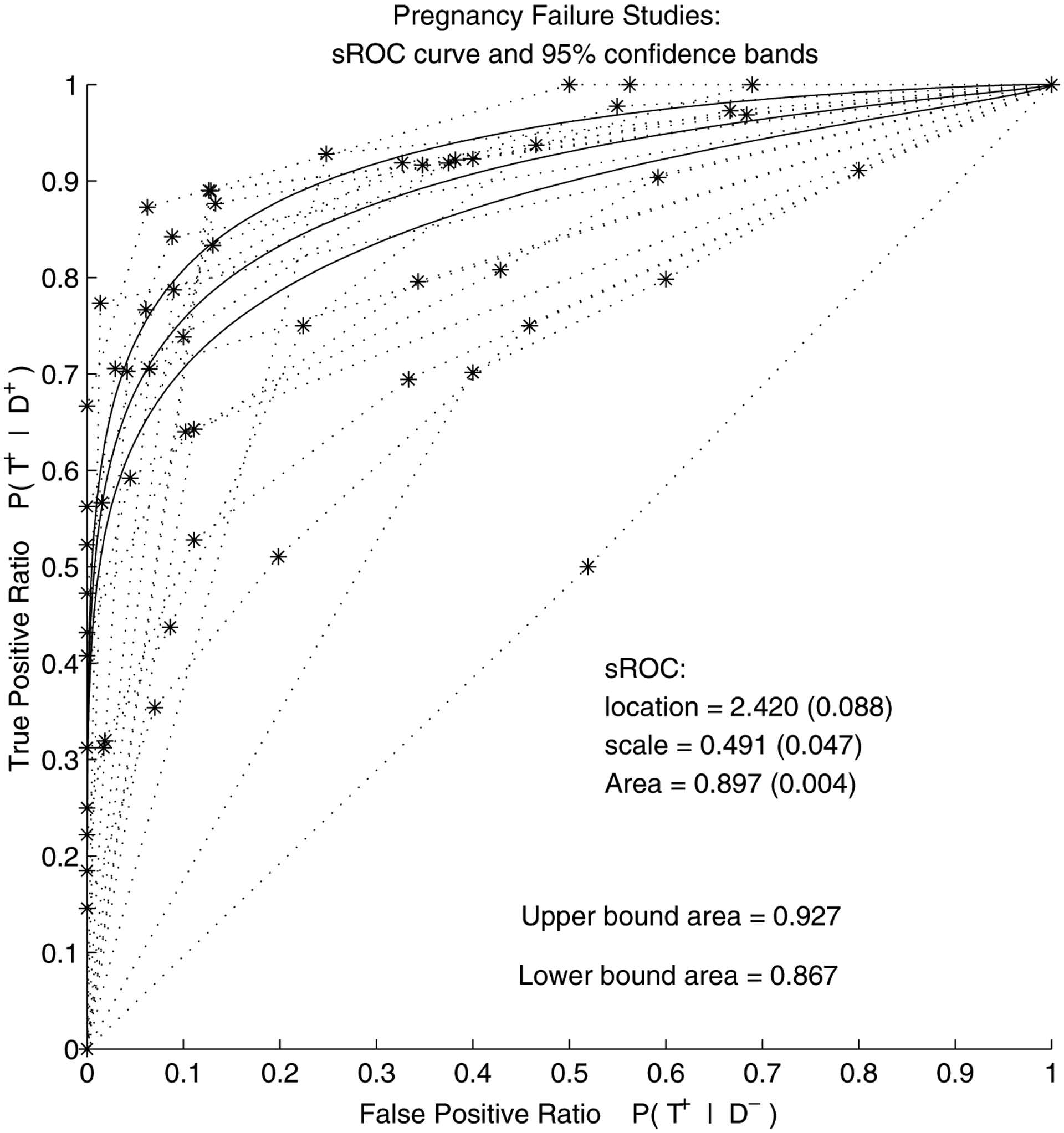
Pregnancy failure meta-analysis (FE model without covariate): summary ROC curve and its 95% confidence pointwise bands (obtained via delta method). The dashed lines are the individual-study empirical ROC curves.

As can be seen from Figure 1, the confidence bands are quite narrow. A combination of a large number of patients and many thresholds used in the studies has contributed to the low values in the asymptotic covariance matrix of the maximum likelihood estimates. Also note that the confidence bands based on the delta method are constrained to be equidistant from the SROC. To adjust for within-study correlation, bootstrap sampling was done in a simple fashion: only the studies were sampled randomly with replacement. The bootstrap standard errors, based on 1000 samples, appear to be slightly larger than the asymptotic standard errors: 0.20 for the location and 0.08 for scale, as shown in Table 2.

The next question of interest in this meta-analysis is whether some variation among studies can be explained by study characteristics such as, in our case, study design. As seen in Table 2, in the model with covariate, the location was estimated at $2.47\left(0.09\right)$, while the scale was estimated at 0.55 (0.05). Both are still significantly different from zero. The coefficient of the study-design covariate, $\gamma$, was estimated to be 0.10 (0.03), indicating a significant difference in the scale estimates between prospective and retrospective studies. Area under the SROC curve for prospective studies was estimated to be $0.87\left(0.01\right)$, while for retrospective studies, it is 0.91 (0.01). The difference is 0.035 and its delta-method standard error is 0.0015. These results are similar to what was found by Mol et al. (1998), who report that retrospective studies have significantly higher accuracy (the reported p-value is less than 0.001). The SROC curves for the two types of studies are shown in Figure 2: retrospective SROC curve lies slightly above the SROC curve for prospective studies. The bootstrap standard errors were again slightly larger than the asymptotic ones: 0.20 for location, 0.09 for scale, and 0.10 for the study indicator estimated parameter (Table 2). Interestingly, the significance of the study covariate is lost when the within-study correlation is accounted for via bootstrap.

Figure 2.

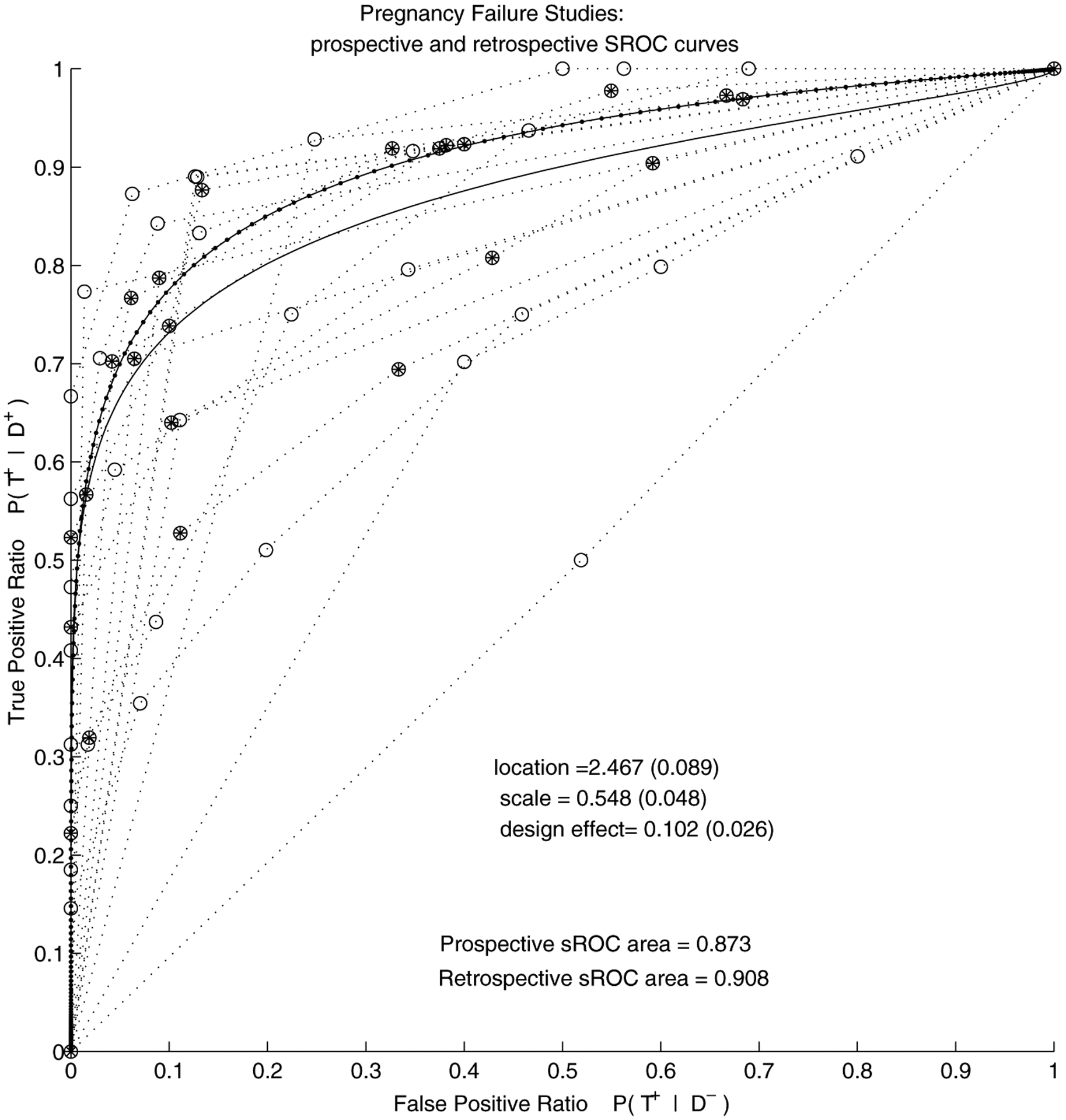
Pregnancy failure meta-analysis (FE model with covariate): Summary ROC curves for 13 prospective and 7 retrospective studies reporting on distinction between pregnancy failure and viable intra-uterine pregnancy. The line with dots and filled circles correspond to retrospective studies and the lines with clear circles correspond to prospective studies.

We repeated our analysis without the apparently outlying study whose ROC curve is close to the diagonal (Darai et al., 1996). The retrospective studies still remained superior: AUC for prospective studies was estimated at 0.89, and for retrospective 0.91. The AUC in the model without covariate increased from 0.897 to 0.901.

5.2. Hierarchical Modeling Approach

The bootstrap analysis has shown that standard errors are inflated when the within-study correlation is taken into account. To compare the models more formally, we use the criterion based on the posterior predictive loss (PPL) function (Gelfand and Ghosh, 1998). Conceptually close to the Akaike Information Criterion, it favors optimal combinations of fit and parsimony. We compare 4 models, fixed-effect (FE) and hierarchical models (HM) with and without the study design covariate. For the FE models, the PPL was computed as if flat priors were used for all parameters. The PPL was much lower in the HM (25,848 for the model without, and 25,931 for the model with covariate) than in the FE models (39,080 without and 38,566 with covariate), suggesting that accounting for study-level variation was beneficial. Adding the covariate to the basic HM did not change the PPL much, suggesting that the covariate was not as beneficial as in the FE setting.

The BUGS code and details of the Gibbs sampling scheme can be obtained from the authors on request. Convergence was assessed in two ways: via the modified Geweke’s statistic (Geweke, 1992), comparing early and late portions of the chain, and via the Gelman and Rubin statistic, comparing the within to the between variability of chains started at dispersed initial points (Gelman et al., 1995). After thinning, the approximate joint posterior distribution of the parameters of interest $(\alpha ,\beta ,\gamma )$ exhibits slight correlation between the mean scale $\alpha$ and the mean location parameter $\beta$, but not between $\beta$ and scale regression coefficient $\gamma$, nor between $\alpha$ and $\gamma$. The marginal distributions of $\alpha ,\beta$ and $\gamma$ are quite symmetric, resembling normal distributions. The marginals of the variances of the scale and location parameters, ${\sigma }_{\alpha }^2$ and ${\sigma }_{\beta }^2$, resemble gamma distributions, as expected.

As seen in Table 2, in the HM with covariate, the posterior mean of all location parameters, ${\mu }_{\beta }$, is estimated to be 2.28, with the $95\%$ posterior credible interval (CI) of $\left(\mathrm{1.81,2.76}\right)$. The estimated posterior mean of all scale parameters, ${\mu }_{\alpha }$, is 0.48, with the $95\%$ posterior CI $\left(\mathrm{0.34,0.62}\right)$. For the model without covariate, the situation is almost identical: the posterior mean of ${\mu }_{\beta }$ is 2.29, with the $95\%$ CI $\left(\mathrm{1.83,2.76}\right)$, while the estimate of ${\mu }_{\alpha }$ is 0.49, with the $95\%$ posterior CI $\left(\mathrm{0.33,0.63}\right)$. These point estimates are close to the fixed-effect estimates, but the credible intervals are wider than the corresponding confidence intervals, as expected. For the model with covariate, the posterior median of the location variance ${\sigma }_{\beta }$ is 0.89, with the $95\%$ posterior CI $\left(\mathrm{0.62,1.35}\right)$, while the scale variance ${\sigma }_{\alpha }$ is 0.11, with the $95\%$ posterior CI $\left(\mathrm{0.06,0.27}\right)$. Once again, these are almost identical in the model without covariate. The posterior mean of the design covariate, $\gamma$, is −0.02, very close to zero, with the $95\%$ posterior CI $(-\mathrm{0.16,0.12})$. As indicated by the bootstrap analysis, once the within-study correlation is accounted for, there seem to be no difference between prospective and retrospective studies.

The sensitivity of the posterior estimates to choice of priors was examined using four different priors for the variances of study location and scale parameters (Table 3). Of interest is to see how the posterior estimates change with the varying degrees of informativeness in the prior distributions. In addition to the originally used $ℐ𝒢\left(\mathrm{0.01,0.01}\right)$, we place a more vague prior $ℐ𝒢\left(\mathrm{0.001,0.001}\right)$ first, then the more informative $ℐ𝒢\left(\mathrm{0.1,0.1}\right)$ next, and finally, the most informative $ℐ𝒢\left(\mathrm{1,1}\right)$ for the scale variance, and $ℐ𝒢\left(\mathrm{1,0.1}\right)$ for location variance. The last pair was chosen to match the observed ranges of the individual-study scale and location parameter estimates from each separate study. As seen in Table 3, all parameter estimates remain robust to different prior specifications, except for the variance-of-scale parameters, ${\sigma }_{\alpha }^2$. The posterior distribution of this variance seems to depend strongly on the prior: the more informative and more concentrated away from zero the inverse gamma density, the larger the posterior median of the scale variance. This is not unexpected, however, given that seven of the studies in the meta-analysis only report 2 tables, and thus only support the estimation of one of the ROC parameters.

Table 3.

Sensitivity analysis for the models used in the meta-analysis of serum progesterone diagnostic accuracy studies. Posterior means and 95% HPD intervals for hierarchical model parameters under four different priors. All priors, except ℐ𝒢(1,0.1) have mean 1.

	${\mathit{\sigma }}_{\mathit{\alpha }}^2,{\mathit{\sigma }}_{\mathit{\beta }}^2~\mathcal{I}\mathcal{G}$	${\mathit{\sigma }}_{\mathit{\alpha }}^2,{\mathit{\sigma }}_{\mathit{\beta }}^2~\mathcal{I}\mathcal{G}$	${\mathit{\sigma }}_{\mathit{\alpha }}^2,{\mathit{\sigma }}_{\mathit{\beta }}^2$	${\mathit{\sigma }}_{\mathit{\alpha }}^2~\mathcal{I}\mathcal{G}\left(\mathrm{1,1}\right)$
	$\left(\mathrm{0.001,0.001}\right)$	$\left(\mathrm{0.01,0.01}\right)$	$~\mathcal{I}\mathcal{G}\left(\mathrm{0.1,0.1}\right)$	${\mathit{\sigma }}_{\mathit{\beta }}^2~\mathcal{I}\mathcal{G}\left(\mathrm{1,0.1}\right)$
Pregnancy failure; with covariate
${\mu }_{{\alpha }_k}$	0.55 (0.43, 0.71)	0.48 (0.34, 0.62)	0.59 (0.39, 0.81)	0.62 (0.32, 0.93)
${\sigma }_{{\alpha }_k}$	0.07 (0.02, 0.26)	0.11 (0.06, 0.27)	0.25 (0.15, 0.45)	0.49 (0.34, 0.78)
${\mu }_{{\beta }_k}$	2.40 (1.92, 2.93)	2.28 (1.81, 2.76)	2.46 (1.95, 3.05)	2.49 (2.00, 3.06)
${\sigma }_{{\beta }_k}$	0.94 (0.65, 1.44)	0.89 (0.62, 1.35)	0.96 (0.63, 1.54)	0.86 (0.51, 1.47)
$\gamma$	−0.01 (−0.14, 0.13)	−0.02 (−0.16, 0.12)	−0.01 (−0.21, 0.18)	−0.02 (−0.29, 0.27)
Pregnancy failure; without covariate
${\mu }_{{\alpha }_k}$	0.49 (0.34, 0.59)	0.49 (0.33, 0.63)	0.48 (0.29, 0.66)	0.47 (0.28, 0.67)
${\sigma }_{{\alpha }_k}$	0.05 (0.02, 0.16)	0.12 (0.05, 0.25)	0.22 (0.13, 0.43)	0.47 (0.33, 0.73)
${\mu }_{{\beta }_k}$	2.34 (1.86, 2.81)	2.29 (1.83, 2.76)	2.28 (1.82, 2.79)	2.42 (1.94, 2.92)
${\sigma }_{{\beta }_k}$	0.93 (0.65, 1.37)	0.88 (0.61, 1.33)	0.88 (0.59, 1.35)	0.81 (0.48, 1.30)

The mean SROC curve corresponding to the estimated posterior means of all scale and location parameters is shown in Figure 3, separately for prospective and retrospective studies. The estimated area under the SROC curve for prospective studies was 0.89, and for retrospective, 0.88, with their highest posterior density intervals overlapping almost entirely: (0.85, $0.93)$ for prospective and $\left(\mathrm{0.83,0.92}\right)$ for retrospective studies. These results imply that the collection of prospective studies has practically the same accuracy as the retrospective studies. Partial 95% confidence bands found via the “envelope” method over $\left(\mathrm{0.1,0.9}\right)$ FPR range are superimposed over the collection of ROC curves from all iterations in the bottom half of Figure 3. AUC under the lower and upper bound for prospective studies were 0.83 and 0.94, respectively, and 0.83 and 0.93 for retrospective studies. Although not shown, the pointwise confidence bands are very similar to the envelope bands.

Figure 3.

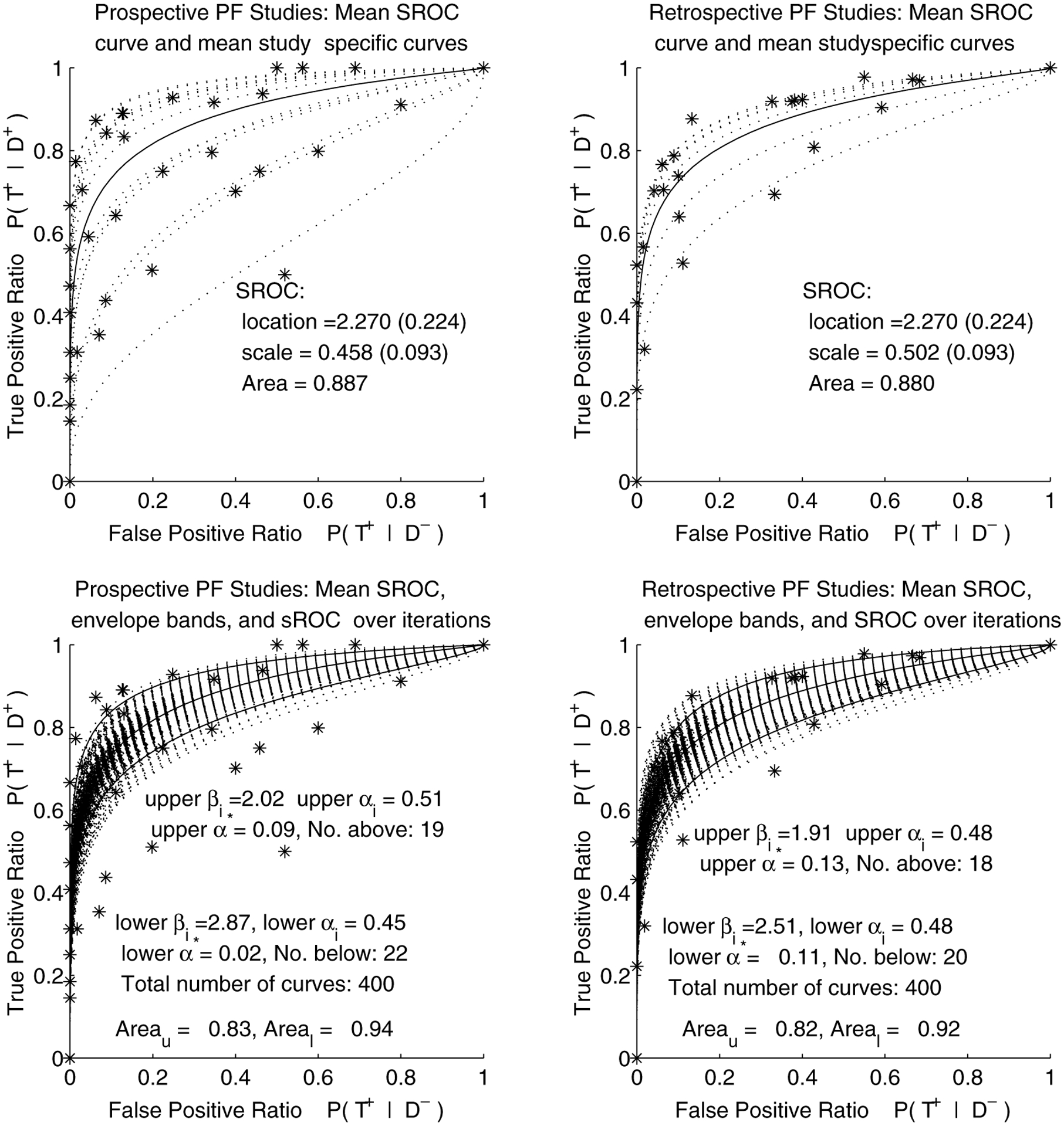
Pregnancy failure meta-analysis (HM with covariate): Mean summary ROC curves for 13 prospective and 7 retrospective studies reporting on distinction between pregnancy failure and viable intra-uterine pregnancy, with envelope $95\%$ bands over $\left(\mathrm{0.1,0.9}\right)$ FPR region.

Removing the outlying study (Darai et al., 1996) from the analysis did not affect our conclusions much. The AUC of prospective studies went from 0.89 to 0.90, and of retrospective studies, from 0.88 to 0.89. The scale estimate changed from 0.46 to 0.54 for prospective, and from 0.50 to 0.58 for retrospective studies.

6. Discussion

We have presented the fixed-effects and Bayesian hierarchical methods for meta-analysis of diagnostic test accuracy studies that report primary test outcomes in a varying number of nonnested ordered categories. This work generalizes the previous research done in this area (Moses et al., 1993; Rutter and Gatsonis, 1995, 2001; Irwig et al., 1994). The fixed-effects approach produces a summary measure of diagnostic accuracy for the studies used in the meta-analysis, and does not take into account the heterogeneity of studies. The hierarchical modeling approach makes it possible to explicitly model the within and between-study variation. It also makes it possible to generalize the findings to a population of studies represented by the ones used in this meta-analysis.

The hierarchical model was fitted using MCMC, yielding a sample from the joint posterior distribution of all parameters in the model and, consequently, a sample of ROC curves. Special attention has to be given to forms and meanings of summaries of such samples of curves; we propose and examine several summary ROC methods in this work. The associated parameter estimates from the fixed-effects and hierarchical models agreed closely, although the credible intervals from the hierarchical model were considerably wider than the intervals in the fixed-effects model, consistently over several choices of variance priors. The difference in the reported diagnostic accuracy between prospective and retrospective studies was significant, based on the results from the fixed-effects model, but did not appear important once the study heterogeneity was taken into account via a hierarchical model. The bootstrap analysis applied to the fixed-effects model confirmed this conclusion.

Several concerns and limitations of this work should be noted. First, we have not explored the possibilities of using covariates to explain some of the differences between study-specific thresholds. The Bayesian model we present, however, could be naturally extended to allow for such covariates. Second, the use of ordinal regression models introduces considerable computational burden. In situations where it is not necessary or feasible to use the primary data from the individual studies, simpler methods for combining ROC curve estimates may be used. These methods can be based on the asymptotic distribution of estimates of ROC parameters or functionals. For example, as suggested by a referee, a weighted average of estimates of the study-specific vector of scale and location parameters could be constructed using the method described in Hall (1992). Hierarchical models using the asymptotic distribution of the study-specific estimates are also the subject of current research. Third, a simulation-based systematic assessment of performance of our model with small samples (small number of studies or small number of patients within studies, or both), as related to small-sample performance of ordinal regression models would be of interest.

In addition, the subset of studies we chose to analyze may have been subject to bias, due both to our selection technique and publication bias. Reassuringly, our results agree with other analyses in the literature of serum progesterone accuracy. Publication bias, however, should be further studied and addressed as suggested by Smith et al. in Stangl and Berry (2000). Moreover, in this article, we have focused our attention on patients with spontaneous conception only, which excluded all those aided with fertility drugs or undergoing assisted reproductive techniques (ART). However, higher risks of pregnancy disorders may be associated with the the hyperstimulatory drugs used in ART, as well as with the conditions that have lead to opting for ART in the first place (Carr and Evans, 2000). Further studies are needed to monitor the accuracy of serum progesterone in diagnosing patients who are undergoing hormonal and fertility treatments, particularly because of the recent increase in the use of ART and contraceptives. An additional concern is that the studies in this meta-analysis are mostly limited to patients who come to clinics with some discomfort, such as, for example, abdominal pain. It is well known, however, that nonviable pregnancies may possibly pass undetected, as their symptoms vary across patients, from those resembling normal periods to severe clinical symptoms. It might be therefore useful if a general-population study addressing progesterone-based test accuracy could be undertaken in the future.