

Abstract
Background and Objective:
The intrinsic electrical material properties of the laminar components of the mammalian peripheral nerve bundle are important parameters necessary for the accurate simulation of the electrical interaction between nerve fibers and neural interfaces. Improvements in the accuracy of these parameters improves the realism of the simulation and enables realistic screening of novel devices used for extracellular recording and stimulation of mammalian peripheral nerves. This work aims to characterize these properties for mammalian peripheral nerves to build upon the resistive parameter set established by Weerasuriya et al. in 1984 for amphibian somatic peripheral nerves (frog sciatic nerve) that is currently used ubiquitously in the in-silico peripheral nerve modeling community.
Methods:
A custom designed characterization chamber was implemented and used to measure the radial and longitudinal impedance between 10mHz and 50kHz of freshly excised canine vagus nerves using four-point impedance spectroscopy. The impedance spectra were parametrically fitted to an equivalent circuit model to decompose and estimate the components of the various laminae. Histological sections of the electrically characterized nerves were then made to quantify the geometry and laminae thicknesses of the perineurium and epineurium. These measured values were then used to calculate the estimated intrinsic electrical properties, resistivity and permittivity, from the decomposed resistances and reactances. Finally, the estimated intrinsic electrical properties were used in a finite element method (FEM) model of the nerve characterization setup to evaluate the realism of the model.
Results:
The geometric measurements were as follows: nerve bundle (1.6mm ± 0.6mm), major nerve fascicle diameter (1.3mm ± 0.23mm), and perineurium thickness (13.8μm ± 2.1μm). The longitudinal resistivity of the endoneurium was estimated to be 0.97Ωm ± 0.05Ωm. The relative permittivity and resistivity of the perineurium were estimated to be 2018 ± 391 and 3.75kΩ ± 981Ωm, respectively. The relative permittivity and resistivity of the epineurium were found to be 9.4x10⁶ ± 8.2x10⁶ and 55.0Ωm ± 24.4Ωm, respectively. The root mean squared (RMS) error of the experimentally obtained values when used in the equivalent circuit model to determine goodness of fit against the measured impedance spectra was found to be 13.0Ω ± 10.7Ω, 2.4° ± 1.3°. The corner frequency of the perineurium and epineurium were found to be 2.6kHz ± 1.0kHz and 368.5Hz ± 761.9Hz, respectively. A comparison between the FEM model in-silico impedance experiment against the ex-vivo methods had a RMS error of 159.0Ω ± 95.4Ω, 20.7° ± 9.8°.
Conclusion:
Although the resistive values measured in the mammalian nerve are similar to those of the amphibian model, the relative permittivity of the laminae bring new information about the reactance and the corner frequency (frequency at peak reactance) of the peripheral nerve. The measured and estimated corner frequency are well within the range of most bioelectric signals, and are important to take into account when modeling the nerve and neural interfaces.
INTRODUCTION
Since the early 1850s, electrical stimulation has been used as a means to modulate the activity within the nervous system. It was initially developed as an intervention to address and, to some degree, treat motor disabilities (1). About a hundred years later in the 1950s, with the advent of solid state electronic devices (2) and later microelectronics (3), the precision and accuracy of delivering electrical stimulation was improved. It was possible to apply the surface intervention with less discomfort and lower electrical power directly to the peripheral nerves through implanted devices to modulate not only sensory-motor function, but also respiratory functions (4), obesity (5), chronic pain (6), and seizures (7). More recent work has seen the development of advanced multi-channel devices such as the FINE (8), MCC (9), LIFE (10), and TIME (11) devices that improve selectivity, tunability, and chronic stability of the therapeutic effect of the device over time.
As devices become more sophisticated and the need grows to increase the operational envelope and stability of the device and therapy; tools to inform rational design of the devices are needed. In-silico methods that model the electrode / structure / nerve relationships are a potentially powerful tool to screen and identify promising electrode / neural interface geometries, and explore stimulation waveforms. Moreover, they can help to suggest potential mechanisms underlying the bioelectric phenomenon related to these methods. The insights provided can inform the designs of advanced implantable neural interfaces, while reducing the number of animals used in the pursuit of improved stimulation selectivity and sensitivity. As devices become more complex, the combination and permutations of the variables within the structures, such as contact size, geometry, and placement also exponentially increase. It becomes impractical to span the variable space using physical or animal experiments. Therefore, the importance of in-silico model informed designs comes to the forefront.
Although in-silico informed design is a powerful tool to meet this growing need, as outlined by Grinberg et al. (12), there remains a large degree of uncertainty in the appropriate values of the parameters to be used within these models. Issues can arise when the material properties, geometric values, and assumptions used in one case are extrapolated to another. These extrapolations lead to errors which degrade the accuracy and the realism of the outcomes coming from the model.
For example, Grinberg et al. (12), ran a meta-analysis for the thickness of human perineurium versus fascicle diameter and found that this was 3% ± 1%. Later, this value was applied to the rat tibial model (13) with the assumption that the cross species and size scales were the same 3%. Another example exists for the temperature coefficient factor, , which is used without direct or indirect validation outside its original context. A value of 1.5 has been found and used repeatedly (14, 15) and is linked back to Hugh Bostock’s 1983 paper (16). Bostock mentions values in relation to either an axoplasmic or leakage conductance temperature correction for the nerve fiber model. Even still the range presented is 1.3 – 1.5, with 1.3 for axoplasmic conductance and 1.4 for leakage conductance values. The is applied to correct temperature effects in the endoneurium and perineurium, and small differences such as 1.5 verses 1.3 results in a nearly 22% difference when correcting temperature effects from 22°C to 37°C.
The first known and last identified impedance measurement of the peripheral nerve laminae was conducted by Weerasuriya et al. in a frog sciatic nerve (17). Although these measurements have never been verified in mammalian models, they have been used repeatedly to date (12–14, 18), either as a direct reference or indirect reference, as no other measures have been found in literature. Despite originating from two different sub-classes of vertebrates, the amphibian peripheral nerve shares many similarities to that of a mammal. The similarities extend to a loose sheath of collagen, the epineurium, surrounding a more densely packed sheath, the perineurium (17, 19, 20). The perineurium is composed of perineurial cells and acts as a diffusion barrier, protecting the fragile and tightly regulated milieu of the endoneurium. The ability of an electrical current to effectively penetrate the nerve bundle is dependent primarily on the complex impedance across the perineurium. The present study was conducted with the intent of characterizing the complex impedance across the perineurium and epineurium of a canine peripheral nerve, specifically the geometrically independent material properties of resistivity and relative permittivity.
MATERIALS AND METHODS
All animal tissue were acquired under the authority and approval of the Indiana University School of Medicine Institutional Animal Care and Use Committee (IUSM IACUC). Tissues were obtained immediately after euthanasia of the animal. Vagus nerves from 5 euthanized canines were extracted and characterized in this study.
Canine Vagal Nerve Extraction
The vagus nerves were extracted following postmortem trachea removal. The nerves were isolated from the connective tissue in the cervical region from the middle cervical ganglia up to the mandible, a length of between 80mm–100mm. Care was taken not to disturb the epineurium and perineurium during this procedure. Once excised, the nerve was placed in an oxygenated Krebs-Henseleit (Composition in mM: NaCl, 113.0; KCl, 4.8; CaCl2, 2.5; KH2PO4, 1.2; MgSO4, 1.2; NaHCO3, 25.0; and glucose, 5.5) solution (21) to keep the nerve viable and prevent drying. All measurements were made at room temperature, 22°C ± 1°C.
Radial Complex Impedance Measurement
The nerve was cut into approximately 25mm–30mm segment lengths to fit in the custom built experimental chamber. The excess nerve length was used to secure the nerve to the experimental chamber, shown in Fig. 1A. The nerve impedance characterization chamber was made by pouring two-part silicone rubber (Silastic 184, Dow Corning, Midland MI) around an assembly of Teflon rods sitting within a glass petri dish. After curing, the Teflon rod assembly was removed leaving a 3mm diameter cylinder channel bisected by a larger 11.25mm diameter by 15.5mm long cylindrical characterization chamber. A cylindrical counter electrode was made forming a thin silver sheet over the larger diameter Teflon rod used to form the characterization chamber and autoplating it in bleach to form a cylindrical Ag/AgCl electrode. The cylindrical Ag/AgCl electrode was placed within the characterization chamber to line and form its curved inner chamber wall. The geometry of the chamber was informed by a series of FEM simulations of the chamber (Comsol v6.0, Comsol Inc, Burlington MA) to determine the minimum length and diameter needed to establish longitudinally uniform and radially symmetrical isopotential shells within the characterization chamber while minimizing the edge fringe effects given a 2.2mm diameter nerve bundle to be characterized.
Figure 1:

A) shows an example setup of the custom recording chamber while the nerve is in place B) is a computer aided drawing (CAD) rendering of the recording chamber, showing the cross-sectional view C) shows a schematic representation of how the current was applied and potentials measured using a four-point measurement technique for characterizing the radial impedances.
Four electrodes were used to characterize the radial impedance of the nerve in a four-point configuration, as shown in Fig. 2. The measured parameters were used to identify components in an electrical equivalent circuit model as shown in the Figure 2. A modified 25-gauge hypodermic needle, bent at a nearly 90° angle with a silicone tube covering the angled section and a small portion of the straight section, was placed down the long axis of the major fascicle of the nerve bundle to deliver current, acting as the working electrode (WE). The current returned through the counter electrode (CE), the large cylindrically formed Ag/AgCl sheet placed at the periphery of the characterization chamber. Teflon insulated 50.8μm diameter platinum-iridium (Pt-Ir) wires (776000, A-M Systems, Carlsbad WA) electrodes, whose insulation was exposed for 1mm and platinized via electrochemical deposition in Kohlrausch’s solution (22), termed platinum black coating, was used as measurement reference electrodes (RE). The intrafascicular measurement electrode (RE1) was attached to and threaded into the nerve together with the WE. The extrafascicular measurement electrode (RE2) was placed within the saline bath of the chamber, aligned with the measurement point of RE1 and in contact with the nerve bundle’s epineurium.
Figure 2:

The bulk electrical equivalent circuit of the four-point measurement radial complex impedance measurement. The top schematic shows the points where the various electrodes are positioned relative to the bulk electrical equivalent model. The Cole-Cole plot of its impedance, a plot of the real impedance versus the imaginary impedance (25), reveals a locus in the form of a depressed semicircle. The variable characterizes the depression of the semicircle’s center point, with the infinite and zero frequency resistances estimated as the intersection of the semicircle with the real axis. The , or constant phase element (CPE), is calculated as a partial of or the radius of the circle, that is one minus the depression amount divided by .
The radial impedance of the nerve bundle was measured using electrochemical impedance spectroscopy (EIS) using the rapid impedance measurement technique (23). Briefly, bandwidth limited noise was passed between the WE and the CE galvanostatically using an electrochemical interface (Model 1287, Solartron, Farnborough UK). The resulting potential drop across the tissue laminae was measured differentially across the measurement electrodes (RE1 – RE2). Both the source waveform and the voltage drop waveform were passed into a two channel gain / filter amplifier (PFA2, Precision Filters Inc, Ithaca NY), prior to digitization by sampling at 500kHz using a 16-bit A/D converter (USB-6361, National Instruments, Austin TX). The acquired time series data was processed in Matlab (2021b, Mathworks, Natick MA) as described in (24) by using an empirical transfer function estimator and compensating for the linear sampling phase error to yield the impedance spectra.
After the initial four-point complex impedance measurement, which characterized the radial impedance of the perineurium in series with the epineurium, a 30-gauge hypodermic needle was used to perforate the perineurium to remove its effects from the impedance measurements. The perforation procedure was repeated until no significant change in impedance was observed.
Longitudinal Complex Impedance Measurement
The longitudinal impedance measurements of the endoneurium were made on 80mm - 100mm long segments of the excised cervical vagus nerve. A pair of 25-gauge needles were transversely placed through the nerve bundle at both ends to act as the WE and CE, while also anchoring the nerve bundle down to a silicone bottomed glass dissection tray to keep the nerve bundle taut. Two 0.25mm - 0.5mm long exposures were made on Teflon insulated 50.8μm diameter Pt-Ir wires which were electroplated with platinum black to form wire electrodes. The wire electrodes were then attached to a tungsten needle and sewn into the nerve fascicle of the canine vagus nerve along its longitudinal axis. The black platinized measurement sites were clearly visible within the nerve fascicle and enabled measurement of the relative displacement of the two electrodes, and position relative to the entry and exit points of the wires in/out of the nerve fascicle (Fig. 3). The longitudinal distance, from entry to exit point for the moving electrode RE2, was about 13mm. These wire electrodes acted as the measurement electrodes RE1 and RE2. To ensure current moved in the longitudinal axis along the nerve, and to keep the nerve from drying out, mineral oil was used as an insulator around the nerve. Differential measurements were made by moving RE2 with respect to RE1 and measuring the impedance between the two points, Fig. 3. Impedance measurements were made at every millimeter increment from 0mm − 12mm separation.
Figure 3:

An image showing the intrafascicular electrode contact placement in the longitudinal impedance measurements. The excised length of vagus nerve was pinned down at its ends to a silicone bottomed dissection tray by 25-gauge stainless steel needles which doubled as the working and counter electrodes (not shown). The nerve bundle was implanted intrafascicularly with a pair of 50.8μm diameter Pt-Ir wire electrodes. The entry and exit locations of the wires were about 13mm apart longitudinally(top electrode exit point not shown). The electrode contacts were displaced with respect to one another at 1mm increments to measure the differential potential within the nerve fascicle originating from the currents sourced between the working and counter electrodes.
The longitudinal impedance of the nerve bundle was measured using the same EIS with the rapid impedance measurement technique as the radial impedance measurement. However, the device setup differed, as it was an early setup. In the place of the Solartron, a custom-built measurement device was used as described by Sempsrott (24). The data was digitized sampling at 130 kHz and 16-bits resolution (USB-6251, National Instruments). The acquired time series data were processed in Matlab (2019a, Mathworks, Natick MA) as described in (24) by using an empirical transfer function estimator and compensating for the linear sampling phase error to yield the impedance spectra.
Nerve Geometry Quantification
The morphology of the nerve cross section was characterized with 5μm sections of nerve immediately adjacent to the segment that was electrically characterized. To minimize degradation of the nerve, the tissues were prepared immediately after the impedance measurements were made. The segment of nerve was cut to a length of 5mm and promptly embedded in a 7mm × 7mm × 5mm disposable base mold (62352–07, EMS Diasum, Hatfield PA) containing Tissue Plus® O.C.T. Compound (23–730-571, Fisher Scientific, Waltham MA).
The embedded nerve samples were removed from the mold and placed onto specimen holders cooled to −20°C and fixed with a layer of O.C.T. compound. The nerve was mounted such that the longitudinal axis of the nerve was normal to the cryostat chuck plate to enable transverse sections of the nerve. Histological sections (~5μm) were made using a cryotome (Frigocut 2800E, Leica Jung) with the box temperature set to between −20°C and −25°C to avoid chunking out, crumbling or chatter in the sections. Specimens were placed onto charged microscope slides (1358W, Globe Scientific Inc., Mahwah NJ), and soaked in a 90% ethanol solution for 15s. Staining was performed on the dried slides using one of two protocols: progressive hematoxylin and eosin (H&E) or toluidine blue. Images were captured using a 10MP digital eyepiece camera (MU1003, AmScope, Irvine CA) on an upright brightfield microscope (DM300, Leica, Wetzlar DE) and with a 4× objective.
Quantification of Electrical Circuit Equivalence
A cylindrical approximation was made to derive an electrically equivalent circuit for the radial impedance measurements, equations 1, 6–9. These were used to yield relative permittivity , corner frequency , resistivity , sheet resistance , and sheet capacitance , respectively of the perineurial or epineurial membrane in the radial direction.
| (1) |
Where , , and are measured perineurium capacitance, outer radius of perineurium or epineurium, thickness of perineurium or epineurium and length of the recording chamber, respectively.
| (2) |
| (3) |
| (4) |
| (5) |
| (6) |
where , , , , and are the angular frequency, CPE, corner frequency, DC frequency resistance, and infinite frequency resistance of the perineurium or epineurium.
| (7) |
| (8) |
| (9) |
The longitudinal impedance spectra and a measurement of the total nerve diameter the longitudinal resistivity of the endoneurium was estimated using equation 10.
| (10) |
In-Silico Modeling of the Custom Impedance Chamber
To compare the results of the ex-vivo experiment a time varying in-silico Comsol model was created. The geometry of the 11 physical nerve bundles were tested. The geometry of each was captured using the parameters measured from the histological measurements. The in-silico nerve model was then placed within a recreation of the custom recording chamber used in the physical measurements, see Fig. 1. A 25-Gauge needle was used as the WE delivering a normal current density of pure-tone sinusoidal waveforms to span the same frequencies used in the physical measurements. The CE was set to ground. As in the physical chamber, the ground had an arc length that spanned 260° of the outer diameter of the recording chamber. The reference electrodes were not modeled as physical objects, but rather as two measurement points in the 3D space. RE1 was measured 1μm from the 25-Gauge needle in the positive x-axis, while RE2 was measured 1μm inside the outer boundary of the fascicle in the same axis as RE1. All boundaries were set to von Neumann condition (insulator) and Comsol’s default tetrahedral meshing was implemented. The fasciclar diameter, perineurium thickness and nerve bundle diameter of the 11 physical cases modeled are listed in Table 1. To yield a singular value, the average of the 11 measurements was quantified. The values derived from the ex-vivo experiments for perineural and epineural conductivities and permittivities are presented in Table 3. Access to the Comsol file can be obtained by reaching the corresponding author of this paper.
Table 1:
Histology Results
| Perineurium | Epineurium | ||||||
|---|---|---|---|---|---|---|---|
| Nerve ID | Major(μm) | Minor (μm) | Ave. Diam (mm) | Thickness (μm) | Ave. Diam (mm) | Thickness (μm) | |
| B91029R | 899.6 | 573.4 | 0.7 | 12.3 | 1.0 | 125 | |
| B91105L1 | 1349.7 | 1214.0 | 1.3 | 14.9 | 1.7 | 186 | |
| B91105L2 | 1153.2 | 1121.4 | 1.1 | 13.0 | 1.7 | 257 | |
| B91105R1 | 1382.9 | 759.7 | 1.1 | 13.7 | 1.2 | 73 | |
| B91112L2 | 787.5 | 662.5 | 0.7 | 10.4 | 1.0 | 115 | |
| B91112L3 | 1321.4 | 1321.3 | 1.3 | 15.1 | 1.8 | 235 | |
| B91112R1 | 954.4 | 839.9 | 0.9 | 11.8 | 1.2 | 169 | |
| B91112R2 | 1148.2 | 743.8 | 0.9 | 11.5 | 1.3 | 187 | |
| C00225L1 | 1802.6 | 1664.6 | 1.7 | 16.7 | 2.3 | 268 | |
| C00225L3 | 2480.9 | 2446.6 | 2.5 | 16.2 | 2.8 | 162 | |
| C00225R2 | 2125.3 | 1433.5 | 1.8 | 15.6 | 2.2 | 227 | |
| Mean | 1.3 | 13.8 | 1.6 | 182.2 | |||
| Std Dev | 0.5 | 2.1 | 0.6 | 61.7 | |||
The results of the histological analysis of the canine nerve trunks after the complex impedance experiment was carried out. The average fascicle diameter of the nerves was 1.3mm ± 0.5mm, the average perineurium thickness was 13.8μm ± 2.1μm, the average nerve bundle diameter was 1.6mm ± 0.6mm and the average epineurium thickness was 182.2μm ± 61.7μm for the sample size of n = 11.
Table 3:
Bulk Material Properties
| Perineurium | Epineurium | |||||||
|---|---|---|---|---|---|---|---|---|
| Nerve ID | ||||||||
| B91029R | 3035.8 | 1987 | 371.9 | 14.3 | 2885.1 | 75.7 | 196,000 | 1110.3 |
| B91105L1 | 3350.7 | 2095 | 499.5 | 12.4 | 2476.6 | 98.1 | 25,759,713 | 7.1 |
| B91105L2 | 2241.3 | 1484 | 292.2 | 10.1 | 5086.5 | 37.7 | 2,342,804 | 200.3 |
| B91105R1 | 3580.9 | 1773 | 492.2 | 11.4 | 2703.4 | 27.6 | 260,191 | 2452.1 |
| B91112L2 | 4114.3 | 2489 | 429.7 | 21.1 | 1683.0 | 50.5 | 8,170,127 | 42.7 |
| B91112L3 | 3835.8 | 2008 | 579.7 | 11.8 | 2273.9 | 90.7 | 3,700,831 | 53.1 |
| B91112R1 | 5706.2 | 2121 | 672.2 | 15.9 | 1446.0 | 45.8 | 10,282,390 | 36.9 |
| B91112R2 | 4730.0 | 2766 | 544.1 | 21.3 | 1349.6 | 62.1 | 5,025,925 | 55.3 |
| C00225L1 | 3193.9 | 2068 | 532.4 | 11.0 | 2716.3 | 53.2 | 18,665,995 | 18.1 |
| C00225L3 | 4579.7 | 1400 | 742.8 | 7.6 | 2794.9 | 25.4 | 14,495,737 | 44.7 |
| C00225R2 | 2895.6 | 2014 | 452.3 | 11.4 | 3070.7 | 38.0 | 14,592,696 | 32.4 |
| Mean | 3751.3 | 2018 | 509.9 | 13.5 | 2589.6 | 55.0 | 9,408,401 | 368.5 |
| Std Dev | 981.3 | 319 | 128.0 | 4.4 | 1020.0 | 24.4 | 8,236,424 | 761.9 |
Using histology data from Table 1, base electrical properties from Table 2 and Eq. 1–9, non-geometrical dependent material properties were calculated for the perineurium and epineurium. Yielding a resistivity of 3751.3Ωm ± 981.3Ωm, a relative permittivity of 2018 ± 319, a sheet resistance of 509.9Ωcm2 ± 128.0Ωcm2, a sheet capacitance of 13.5μF/cm2 ± 4.4μF/cm2 and a corner frequency 2589.6Hz ± 1020.0Hz for the perineurium. For the epineurium, a resistivity of 55.0Ωm ± 24.4Ωm, relative permittivity of 9, 408, 401±8, 236, 424 and a corner frequency 368.5Hz ± 761.9Hz. With a sample size of n = 11.
ANALYSIS
Histiology Analysis
Nerve cross sections were made to measure the geometries used to estimate the bulk electrical properties of the nerve. Analysis was performed in ImageJ (Rasband, W.S., ImageJ, U. S. National Institutes of Health, Bethesda, Maryland, USA, https://imagej.nih.gov/ij/, 1997–2018.) to quantify the minor and major axes of the nerve fascicle as well as the thickness of the perineurium and epineurium. The minor and major axes were averaged to obtain an estimate of the diameter of the nerve fascicle, which was used to approximate the nerve as a cylinder in the calculation of relative permittivities (Eq. 1) and resistivity (Eq. 7). Figure 4 shows the details that were used in determining the perineurium membrane to quantify its thickness and the diameter of the major fascicle.
Figure 4:

In this image a blue dashed circle demarks the boundary of the endoneurium. An elliptical fit was used to estimate the outer diameter. The red arrows indicate a clear perineurial membrane used to estimate the thickness of the perineurial membrane. The green arrows show some intact epineurium where its thickness is estimated.
Radial Complex Impedance
The radial complex impedance measurements were collected as a four-point EIS measurements across the various laminae of the nerve facicle. Initial intact measurements were made, followed by a series of measurements following perforation of the nerve fascicle. Subsequent puncturing of the nerve bundle resulted in decreased impedance magnitude and reduced phase. The effect of the puncturing/perforation can be seen in Fig. 5. The spectra converged as shown in this figure after the 15th puncture.
Figure 5:

Example Bode plot (left) and Cole-Cole plot (right) of the complex impedance measurements made with an intact nerve bundle, followed by perforation using a 30-gauge needle. These measurements identified the leftmost semicircle in the Cole-Cole plot as the likely complex impedance related to the perineurium.
Fig. 5 shows that perforating the nerve fascicle results in changes to the impedance components associated with the leftmost semicircle corresponding with the high frequency reactance of the impedance. This was reasoned to be an effect on changes to the perineurium membrane rather than the epineurium. The perineurium is composed of tight layers and dense collagen (type-III and IV) (26, 27), and is associated with the large DC impedance which attenuates at higher frequencies. Puncturing and perforating the nerve would disrupt its order and integrity to decrease its contribution in the composite impedance. The epineurium is composed of a loose matrix of type-I collagen (26, 27) and is associated with the impedance component with smaller resistivity. When the nerve bundle was punctured with a 30-gauge needle, specific care was used to puncture the perineurium fully, completely penetrating the nerve fascicle. It was assumed that the perineurium membrane would lose more of its complex impedance. In contrast, the epineurium, due to its loose matrix, would mostly recover from the puncture.
With the semicircles of the Cole-Cole plot defined, the data was then fitted to best fit circles as described by Sempstrott (24). An initial circle was fitted in the high frequency range by fitting the peak reactance, highest point of the negative imaginary axis of the perineurium semicircle, up to the highest frequency measured, counterclockwise on the Cole-Cole plots. This fit was considered the first iteration of the perineurium model fit and provided the inputs to Eq. 11, using the same frequency range used to measure the nerve impedance as the input to the model. This created a model estimate of the perineurium complex impedance which was subtracted from the measured data to yield the assumed epineurium complex impedance portion. The remaining component, attributed largely to the epineurium, was also fitted with the circle fit algorithm and the same equation (Eq. 11) was used to describe the epineurium model fit. Next, a recursive fitting paradigm was used where 1) the most recent epineurium model fit was subtracted from the measured complex impedance data, to yield the perineurium portion of the measured data, and 2) the result was fitted to produce the new perineurium model fit. 3) The new perineurium model fit was then subtracted from the measured complex impedance data, to yield the epineurium portion of the measured data. 4) the result was fitted, to produce the new epineurium model fit, and so on. This recursion was repeated until the fitting program converged on a solution that minimized the difference between the measured data and the full model fit (sum of perineurium and epineurium model fits) as shown in Fig. 6. It is important to also view the fit in multiple domains to determine where the fit is adequate or lacking, a representation of the Bode plot, Cole-Cole plot, and the Cole-Cole plot with the frequency axis shown is found in Fig. 7.
Figure 6:

An example of the Cole-Cole plots showing the decomposition of the measured radial complex impedances of the nerve fascicle (blue) to the individual components of the epineurium (green) and perineurium (yellow). The solid lines show fits of the measured data to the electrical impedance model.
Figure 7:

Another example showing the agreement of the non-linear model fit with the measured impedance. A) Shows the Bode plot representation of the measured impedance and the parametric model fit. B) shows the Cole-Cole plot, the projection of the Impedance projected to the real and imaginary plane. C) shows B) as a 3D plot that includes the frequency axis. It similarly shows good agreement between the measured and parametric model fit.
| (11) |
Longitudinal Complex Impedance
Longitudinal complex impedance measurements were collected on a long section of nerve with intrafascicular electrodes spaced at different longitudinal distances on nearly parallel tracks. Measurements were initially taken with the electrodes right next to each other, then RE2 was moved by 1mm intervals and the impedance measurement was repeated for a total of 13 impedance measurements, from 0mm – 12mm separation. The impedance measurements were nearly purely resistive in the frequency spectra observed, Fig. 8. To measure the resistivity of the longitudinal axis of the nerve bundle, the 13 impedance measurements were analyzed at all unique combinations. For example, the resistance when RE2 was located at 0mm was compared to the resistance measured at 1mm – 12mm and that difference divided by the distance resulted in a resistivity measurement (Eq. 10). Looking at all unique combination resulted in 78 measures. The nerve bundle diameter was measured with calipers and found to be roughly 2.2mm. The nerve bundle diameter was used instead of just the fascicle diameter due to the orientation of the WE and CE, allowing current to flow within the fascicle and the epinerium.
Figure 8:

Bode plot of the longitudinal impedance measurements as a function of longitudinal electrode separation from 0mm-12mm. Showing a nearly linearly increase in resistance magnitude with distance of the separation and next to no phase deviation.
In-Silico Modeling of the Custom Impedance Chamber
Within the Comsol simulation, the pure-tone sinusoidal waveforms were simulated for five sinusoidal cycles to allow for the results to settle to a steady-state. The last cycle of both RE1 and RE2 were analyzed to see the phase shift Eq. 12 and magnitude difference Eq. 13 between these two measurement points. For phase shift, the maximum point of each sinusoid was found and the time difference between RE2 and RE1 was taken and multiplied by the current pure-tone frequency and multiplied by 360°. Magnitude difference was calculated by taking the difference between peak-to-peak voltages at and , and dividing by two.
| (12) |
| (13) |
RESULTS
Histology
The radial impedance nerves were all subjected to histological analysis to get specific measurements of the fascicle diameter and perineurium thickness. These results are found in Table 1.
Radial Impedance
Following the recursive fitting paradigm in the methods section, best fit models were developed, and the base electrical properties can be found in Table 2. From these values using Eq. 1–9 and Table 1, it was possible to derive non-geometrically dependent or bulk material properties of the perineurium, found in Table 3.
Table 2:
Equivalent Electrical Components
| Perineurium | Epineurium | Total RMS Fit | ||||||||
|---|---|---|---|---|---|---|---|---|---|---|
| Nerve ID | C (nf) | C (nF) | RMS Mag | RMS Pha | ||||||
| B91029R | 50.5 | 0.89 | 1091.6 | 37.7 | 579 | 0.89 | 247.7 | 20.7 | 28.8 | 2.2 |
| B91105L1 | 76.8 | 0.81 | 837.0 | 27.5 | 87,185 | 0.48 | 258.5 | 1.9 | 10.7 | 1.6 |
| B91105L2 | 55.2 | 0.82 | 567.2 | 33.3 | 5,416 | 0.75 | 146.7 | 2.3 | 3.7 | 0.2 |
| B91105R1 | 58.8 | 0.84 | 1001.2 | 45.2 | 1,756 | 0.80 | 37.0 | 0.8 | 10.7 | 5.6 |
| B91112L2 | 73.4 | 0.80 | 1288.0 | 53.1 | 25,568 | 0.90 | 145.7 | 2.9 | 7.5 | 1.3 |
| B91112L3 | 74.8 | 0.82 | 935.7 | 24.0 | 10,484 | 0.87 | 285.9 | 2.3 | 14.5 | 1.1 |
| B91112R1 | 68.7 | 0.82 | 1602.0 | 42.5 | 27,728 | 0.97 | 155.5 | 5.2 | 9.4 | 0.8 |
| B91112R2 | 96.9 | 0.80 | 1217.3 | 21.6 | 13,009 | 0.94 | 221.3 | 8.9 | 23.8 | 1.2 |
| C00225L1 | 91.9 | 0.78 | 637.9 | 1.2 | 59,758 | 0.74 | 147.2 | 0.1 | 6.4 | 0.8 |
| C00225L3 | 91.1 | 0.80 | 625.1 | 1.9 | 101,181 | 0.84 | 35.2 | 3.0 | 18.5 | 1.5 |
| C00225R2 | 98.0 | 0.80 | 528.9 | 2.1 | 55,361 | 0.73 | 88.8 | 0.2 | 8.6 | 10.3 |
| Mean | 76.0 | 0.82 | 939.3 | 26.4 | 35,275 | 0.81 | 160.9 | 4.4 | 13.0 | 2.4 |
| Std Dev | 16.9 | 0.03 | 342.4 | 18.3 | 35,386 | 0.14 | 85.7 | 6.0 | 7.8 | 3.0 |
Using semicircle fits of the Cole-Cole plots, equivalent electrical model values were calculated as shown in this table. This yielded a perineurium capacitance of 76.0nF ± 16n.9F, a constant phase element of 0.82 ± 0.03, a low frequency resistance of 939.3Ω± 342.4Ω, and a high frequency resistance of 26.4Ω± 19.3Ω. For the epineurium, a capacitance of 35, 275nF ± 35, 386nF, a constant phase element of 0.81 ± 0.14, a low frequency resistance of 160.9Ω ± 85.7Ω, and a high frequency resistance of 4.4Ω ± 6.0Ω. Both laminae were calculated with a sample size of n = 11. The goodness of fit was calculated as an RMS of the magnitude, 13.0Ω ± 7.8Ω, and the phase, 2.4° ± 1.3°.
Longitudinal Impedance
The endoneurium shows little reactivity and is mostly resistive. This is in line with what has been previously shown, exhibited in Fig. 8 and again in Fig. 9. In this figure, the spread of the resistivity is shown along with histograms to indicate the phase and magnitude deviations. This strongly suggests that the potentials within the nerve fascicles were planar, such that the isopotential planes were perpendicular to the longitudinal axis of the nerve. Given the planar arrangement of the isopotentials within the nerve, there would be little leakage of current outside the nerve fascicle. Thus little to no current would be flowing through the perineurium or epinerium and the measurement is purely attributable to the longitudinal impedance of the endoneurium.
Figure 9:
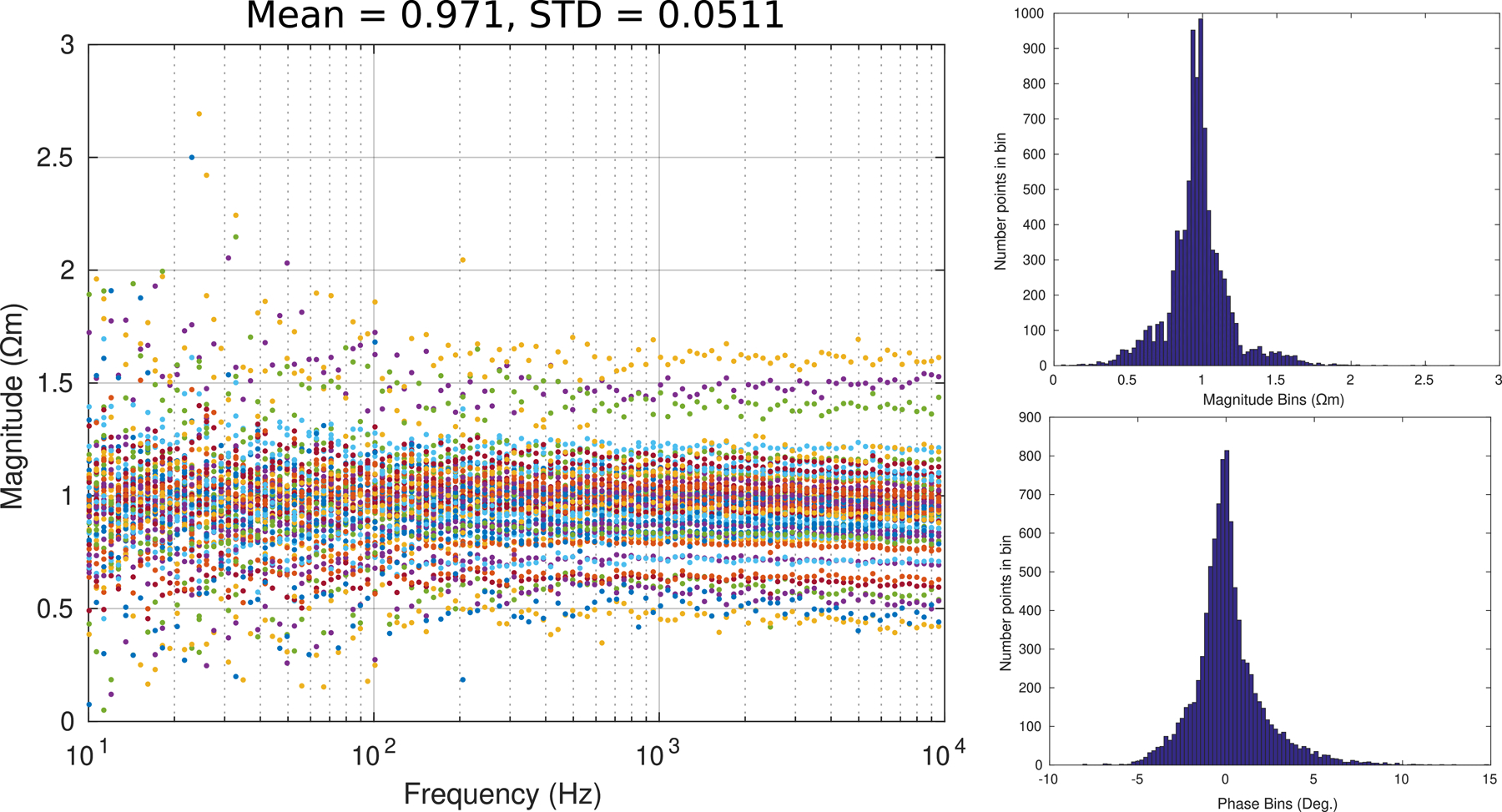
Using Eq. 10, the resistivity was calculated for the endoneurium using the entire nerve diameter of roughly 2.2mm to yield a of 0.971Ωm ± 0.0511Ωm, n = 78 where the magnitude and phase histograms showing a rather tight distribution.
In-Silico Modeling of the Custom Impedance Chamber
These results from Eq. 12 and 13 were used to make a Bode plot and a Cole-Cole plot which was used to directly compare to measured results of the total nerve bundle impedance (perineurium and epineurium), Fig. 10. The RMS error was calculated and found to be 191.7Ω ± 155.5Ω, 15.2° ± 8.6° (Table 4).
Figure 10:

Shows a comparison between an ex-vivo impedance measurement of the unpunctured nerve bundle against the pure tone impedance Bode plots obtained from linear Comsol models (without depression or frequency dependent phase elements). The intent of this experiment was to test the generalizability of the mean bulk electrical parameters when applied to a specific geometry using strictly linear model components, applied in a use case in FEM environments such as Comsol. All three models use the geometry quantified for the experimentally measured nerve (B91112L3) in Table 1. The model using the new experimentally obtained values (red) uses the mean bulk electrical parameter values found in Table 3. The yellow and purple lines are linear models based on current widely-used literature. Both the yellow and purple lines have resistivity of 476Ωm and 12Ωm for perineurium and epineurium, respectively (12). The yellow line uses (, saline) and purple (, from (28)). The model implemented using the mean bulk electrical properties (red) captures most of the characteristics of the nerve impedance in the frequencies <10kHz (neural, muscular bioelectric bandwidth). Whereas, the models based on current literature values remain largely resistive in nature throughout the spectral bandwidth up to and including the neural bandwidth (<10kHz), and do not capture characteristics of the impedance of the actual nerve bundle.
Table 4:
Comsol Model Error
| RMS Error | ||
|---|---|---|
| Nerve ID | Mag (Ω) | Pha (Ω) |
| B91029R | 142.5 | 17.5 |
| B91105L1 | 116.1 | 18.2 |
| B91105L2 | 301.7 | 17.6 |
| B91105R1 | 66.2 | 11.6 |
| B91112L2 | 82.2 | 10.5 |
| B91112L3 | 61.4 | 18.6 |
| B91112R1 | 335.0 | 12.8 |
| B91112R2 | 121.7 | 14.8 |
| C00225L1 | 212.3 | 33.0 |
| C00225L3 | 86.8 | 37.6 |
| C00225R2 | 222.7 | 35.3 |
| Mean | 159.0 | 20.7 |
| Std Dev | 95.4 | 9.8 |
RMS error of the magnitude (159.0Ω ± 20.7Ω) and phase (95.4° ± 9.8°) when comparing the Comsol model, using the specific geometry and average bulk properties, and the ex-vivo data.
DISCUSSION AND CONCLUSION
Prior work by others calculated the sheet resistance and sheet capacitance for frog sciatic nerve perineurium (17). The sheet resistance in was 478Ωcm2 agrees with the measurements made in the present work. Our work confirms that these amphibian values can be correctly applied and extrapolated to mammalian models (12–14, 18). The relative permittivity of perineurium was assumed to be near the value for saline for many models over the years (18). Weerasuriya et al. alludes to a similar sheet capacitance but never reports on a relative permittivity (17). In their study, larger and smaller capacitances were calculated. The smaller capacitance, 0.08μF/cm2, was hypothesized as the capacitance of the perineurium as a whole, and the perineurium was estimated to be due to roughly six layers as conjectured by Shinowara et al. (29). With a specific capacitance for a cell of 0.48μF/cm2 (30) per layer a total sheet capacitance of 0.08μF/cm2 can be calculated, and is likely largely contributed by the perineurium. The larger capacitance was assumed to be the intracellular material between the endoneurium and characterizing electrode, thus the material that was in series with the perineurium. Inspite of the large variability in measurements, 2.7μF/cm2 – 29.5μF/cm2, Weerasuriya et al.’s larger capacitance compares closely with the sheet capacitance measured in this work for the perineurium, 9.6μF/cm2. This suggests that that there were likely errors in Weerasuriya et al’s assumptions and hypothesis. That is, the second capacitance range should have been associated with the perineurium itself and not the intracellular material between and in series with the perineurium.
Due to the nature of the experiment, it was challenging to obtain pristine cross sections of nerve bundle at the location in which the measurements were taken. This was a direct result of the puncturing/perforation process to decompose the impedance components related to each layer of the nerve bundle. The process led to erratic geometries for both the perineurium and the epineurium. Additionally, as a limitation of the study, the gold standard for peripheral nerve morphology was not performed. The gold standard is a glutaraldehyde-fixed, 1% osmium tetroxide post-fixed, semi-thin (i.e. 0.5– 1 micron thick) plastic/ epoxy resin-embedded sections stained with toluidine blue. In future work, this standard should be performed, where sectioned nerve bundles can be cryopreserved in O.C.T. until all the nerve bundles are ready to be processed.
If the experiment were to be revisited, measurements with both the fascicle and epineurium intact and another set with the epineurium stripped from the major fascicle could be a solution to limit the confounding issue of a difficult to measure epineurial geometry. An additional step should be considered to carefully separate and remove the fat from the epineurium to allow for a more homogenous nerve measurement. These modifications were considered, but rejected in our work since stripping the nerve bundle would be an extremely invasive surgical step that could radically alter the geometry of the nerve fascicle. The direction that minimized distortion whilst including the possibility to measure the contribution of the epineurium was taken.
A concern related to impedance measurements is the presence of parasitic capacitances in the cabling, setup and electronics that can lead to large errors in measurements. This manifests itself as a decrease in the magnitude as the signal shorts across the capacitor at large enough frequencies to allow for transduction. The experimental setup used measures and compensates for these parasitic components. Looking at Fig. 8, it can be seen that across the frequency range from 1Hz to 10kHz both magnitude and phase, in the longitudinal setup, remain linear even at magnitudes of around 4kΩ. Moving forward towards the radial impedance setup data was analyzed up to 100kHz with a , the smaller real magnitude will at least double the corner frequency of the parasitic capacitance effect. Assuming the parasitic capacitance effect began at just above 10kHz (worst case scenario), in the longitudinal measurement case, it would be expected that there would be another reactive portion of the impedance spectrum from 20kHz and greater. However there is no such evidence of this in the measurements (see Fig. 7). Give the relatively low impedances in these measurements, parasitic capacitance should become an issue at higher frequencies ( and regions). Even at the impedances measured parasitic capacitance could invade measurements in the dispersion region of the spectrum. However, prior to this work, considerable effort was made to characterize and reduce the effects of parasitic capacitance. Given that the impedance using the same equipment for characterizing radial and longitudinal impedance showed that there was little to no phase detected in the longitudinal impedance case in contrast to the radial impedance measurements despite magnitude values in similar regimes, we conclude that the measurements reflect true measurements rather than those related to instrumentation. The effects of instrumental parasitic capacitance could be made to show itself with samples having much larger impedances and/or characterization at higher frequencies.
Due to the large permittivity value predicted for the epineurium, a Comsol model was created to use these values to see if it produced predictions that captured the essence of the physical measurements. Fig. 10 shows that the results from using this large permittivity were not outlandish. As a comparison to literature values (9, 28), resistivity of 12Ωm and 476Ωm were used for epineurium and perineurium,respectively, and a relative permittivity from the dispersion at 80 for both laminae. Nonetheless, the Comsol model in 10 should be thought of as a best case linear approximation that can be used with linear resistive/capacitive FEM models. It does not take into account the non-linear component, the constant phase element characterized by , which exists in both epineurium and perineurium laminae. These large permittivity values however fit well within the dispersion range indicated in (31). This dispersion range is around DC to a few 10s of kHz, the range of measurements presented in this paper. Miklavčič et. al. also provide a table of values that they collected from many papers and report that gray and white matter having relative permittivities in the 10s of millions making the three million permittivity value calculated here within a reasonable range (31).
These newly measured values help to explain differences between experimental observations and models related to the mechanisms of kHFAC block and the novel LFAC block discovered in our lab in 2013 (32). Previous simulations (12, 18, 33) using a relative permittivity of saline, around 80 (34) resulted in a corner frequency well beyond anything that is experimentally measured. Using a relative permittivity of 1130 (28) did bring the corner frequency within scope, < 100kHz, but lacked the reactance in the Cole-Cole plot in Figure 10. This would mean that the resistivity would need to be higher and thus the relative permittivity as well. However, with the new values of the relative permittivity and resistivity, the corner frequencies of the perineurium, 2.6kHz ± 1.0kHz, and epineurium, 368.5Hz ± 761.9Hz, come within the frequency of interest and suggest a range of frequencies that can short the electrical resistance of the perineurium at signals greater than 2.6kHz and epineurium above 370Hz. This means that kHFAC block works directly on the impedance of the nerve fiber since the frequencies used are above these corner frequencies of the nerve bundle laminae. Since the perineurium and epineurium are shorted, current from the stimulating electrode flows throughout the volume contained by the cuff electrode, a much larger volume than that contained within the nerve bundle. In the case of LFAC block, a small amount of current penetrating the perineurium wall, with large longitudinal potentials forming in the gap between the cuff electrode’s inner wall and outer surface of the perineurium. This sets up a longitudinal potential that is mirrored within the nerve fascicle and causes a large potential gradient to form within the nerve fascicle.
There is currently a general a lack of convergence between modeled and experimentally observed neural recordings. Although experimental observations qualitatively follow in-silico predictions, quantitative agreement of the results generally fail to converge making it difficult to trust the model. Moreover, there are instances where the in-silico predictions diverge from experimentally measured results. For example, Qiao and Yoshida predicted that the spectral energy of single fiber action potentials (SFAPs) measured with intrafascicular electrodes should mirror the spectral energy of the single fiber action current. These predictions expected energy to extend into the 10kHz – 100kHz (32, 33). However, in-vivo measurements of SFAPs have spectral energies containing only two (3kHz and 6kHz peaks) of the four power spectral density peaks (33, 35). The predictions, however, assumed a purely resistive model. Considering results in the present paper that place the corner frequency of the nerve fascicle at 2.6kHz brings the experimental measurements and in-silico predictions into alignment and explains the missing spectral energy of the SFAP. The neural recording energy below the corner frequency is trapped within the perineurium whereas the higher frequency energy escapes the perineurium into the surroundings, greatly attenuating the signal.
This study set out to refine the values of resistivity and permittivity for a mammalian model over the existing amphibian model used for many simulations. Furthermore, it was hoped that a geometrically independent value could be derived such that a bulk property of perineurium and epineurium could be used for any geometry of nerve bundles in simulations hereafter. We found that values in the mammalian nerve agreed with earlier measurements for the conductivity taken from amphibian models but the permittivity, the reactive portion of the impedance, has been shown to be much larger, thus moving the corner frequencies of the nerve bundle as a whole to lower, more interesting frequencies. Furthermore, bulk electrical properties were calculated and extended to include the relative permittivity of the perineurium and epineurium. This enables the calculation of the reactance of the nerve bundle laminae in future models without limiting their geometries to cylindrical nerve models. The ability to model more realistic nerve geometries with the inclusion of the reactance of the perineurium could bring greater realism to in-silico predictions, better convergence of these predictions to experimental measures, explanation of controversial bioelectrical phenomena, and development of new techniques that take advantage of the transient behavior of nerve tissues.
Figure 11:

ACKNOWLEDGMENTS
This work was made possible through the cooperation with Dr. Susan Gunst and her lab for providing the tissue. The authors would like to thank Awadh Alhawwash for his help with the surgical cut down and extraction of the nerve tissues. We acknowledge useful discussions with R. Sarpeshkar. The authors acknowledge Hunter Cox, Tyler Fears, and Tyler Johnson for help with the preparation and preliminary analysis of the peripheral nerve sections. This work was funded in part by an Exploratory Research Grant from Galvani Bioelectronics (#100040339) and a NIH Trailblazer R21 Research Grant (R21EB028469). The Authors also acknowledge the Department of Biomedical Engineering for support of M. Ryne Horn’s Research Assistantship.
Footnotes
CONFLICT OF INTEREST
Rizwan Bashirullah and Mike Carr are employees of Galvani Bioelectronics and collaborators on the earlier phases of this work supported by Galvani Bioelectronics.
REFERENCES
- 1.Reynolds JR, 1855. Report upon the Electro-Physiological Researches of Dr. Duchenne. Br Foreign Med Chir Rev, 15(29):138–151. [PMC free article] [PubMed] [Google Scholar]
- 2.Herrick JF, 1962. History of Bio-Medical Electronics Art. Proceedings of the IRE, 50(5):1173–1177. ISSN 2162-6634. doi: 10.1109/JRPROC.1962.288069. Conference Name: Proceedings of the IRE. [DOI] [Google Scholar]
- 3.Meindl JD, 1982. Microelectronics and computers in medicine. Science, 215(4534):792–797. ISSN 0036-8075. doi: 10.1126/science.7036345. [DOI] [PubMed] [Google Scholar]
- 4.Creasey G, Elefteriades J, DiMarco A, Talonen P, Bijak M, Girsch W, and Kantor C, 1996. Electrical stimulation to restore respiration. Journal of rehabilitation research and development, 33:123–32. [PubMed] [Google Scholar]
- 5.Dalton B, Campbell IC, and Schmidt U, 2017. Neuromodulation and neurofeedback treatments in eating disorders and obesity. Current Opinion in Psychiatry, 30(6):458–473. ISSN 1473-6578. doi: 10.1097/YCO.0000000000000361. [DOI] [PubMed] [Google Scholar]
- 6.Barolat G, Ketcik B, and He J, 1998. Long-term outcome of spinal cord stimulation for chronic pain management. Neuromodulation: Journal of the International Neuromodulation Society, 1(1):19–29. ISSN 1094-7159. doi: 10.1111/j.1525-1403.1998.tb00027.x. [DOI] [PubMed] [Google Scholar]
- 7.Ben-Menachem E, Mañon-Espaillat R, Ristanovic R, Wilder BJ, Stefan H, Mirza W, Tarver WB, and Wernicke JF, 1994. Vagus Nerve Stimulation for Treatment of Partial Seizures: 1. A Controlled Study of Effect on Seizures. Epilepsia, 35(3):616–626. ISSN 1528-1167. doi: 10.1111/j.1528-1157.1994.tb02482.x. _eprint: 10.1111/j.1528-1157.1994.tb02482.x. [DOI] [PubMed] [Google Scholar]
- 8.Tyler DJ, 1999. Functionally selective stimulation of peripheral nerves: Electrodes that alter nerve geometry. Ph.D, Case Western Reserve University, United States – Ohio. ISBN: 9780599416321. [Google Scholar]
- 9.Choi A, Cavanaugh J, and Durand D, 2001. Selectivity of multiple-contact nerve cuff electrodes: a simulation analysis. IEEE Transactions on Biomedical Engineering, 48(2):165–172. ISSN 0018-9294. doi: 10.1109/10.909637. [DOI] [PubMed] [Google Scholar]
- 10.Malagodi MS, Horch KW, and Schoenberg AA, 1989. An intrafascicular electrode for recording of action potentials in peripheral nerves. Ann Biomed Eng, 17(4):397–410. ISSN 0090-6964. [DOI] [PubMed] [Google Scholar]
- 11.Boretius T, Badia J, Pascual-Font A, Schuettler M, Navarro X, Yoshida K, and Stieglitz T, 2010. A transverse intrafascicular multichannel electrode (TIME) to interface with the peripheral nerve. Biosensors and Bioelectronics, 26(1):62–69. ISSN 0956-5663. doi: 10.1016/j.bios.2010.05.010. [DOI] [PubMed] [Google Scholar]
- 12.Grinberg Y, Schiefer M, Tyler D, and Gustafson K, 2008. Fascicular Perineurium Thickness, Size, and Position Affect Model Predictions of Neural Excitation. IEEE Transactions on Neural Systems and Rehabilitation Engineering, 16(6):572–581. ISSN 1534-4320. doi: 10.1109/TNSRE.2008.2010348. [DOI] [PMC free article] [PubMed] [Google Scholar]
- 13.Peña E, Pelot NA, and Grill WM, 2021. Non-monotonic kilohertz frequency neural block thresholds arise from amplitude- and frequency-dependent charge imbalance. Scientific Reports, 11. ISSN 2045-2322. doi: 10.1038/s41598-021-84503-3. [DOI] [PMC free article] [PubMed] [Google Scholar]
- 14.Pelot NA, Behrend CE, and Grill WM, 2019. On the parameters used in finite element modeling of compound peripheral nerves. Journal of neural engineering, 16(1):016007. ISSN 1741-2560. doi: 10.1088/1741-2552/aaeb0c. [DOI] [PMC free article] [PubMed] [Google Scholar]
- 15.Frieswijk TA, Smit JPA, Rutten WLC, and Boom HBK, 1998. Force-current relationships in intraneural stimulation: role of extraneural medium and motor fibre clustering. Medical and Biological Engineering and Computing, 36(4):422–430. ISSN 1741-0444. doi: 10.1007/BF02523209. [DOI] [PubMed] [Google Scholar]
- 16.Bostock H, 1983. The strength-duration relationship for excitation of myelinated nerve: computed dependence on membrane parameters. The Journal of Physiology, 341:59–74. ISSN 0022-3751. [DOI] [PMC free article] [PubMed] [Google Scholar]
- 17.Weerasuriya A, Spangler RA, Rapoport SI, and Taylor RE, 1984. AC impedance of the perineurium of the frog sciatic nerve. Biophys J, 46(2):167–174. ISSN 0006-3495. [DOI] [PMC free article] [PubMed] [Google Scholar]
- 18.Behkami S, Frounchi J, Ghaderi Pakdel F, and Stieglitz T, 2018. Simulation of effects of the electrode structure and material in the density measuring system of the peripheral nerve based on micro-electrical impedance tomography. Biomed Tech (Berl), 63(2):151–161. ISSN 1862-278X. doi: 10.1515/bmt-2016-0089. [DOI] [PubMed] [Google Scholar]
- 19.Reale E, Luciano L, and Spitznas M, 1975. Freeze-fracture faces of the perineurial sheath of the rabbit sciatic nerve. J Neurocytol, 4(3):261–270. ISSN 0300-4864, 1573-7381. doi: 10.1007/BF01102112. [DOI] [PubMed] [Google Scholar]
- 20.King R, 1999. Atlas of Peripheral Nerve Pathology, volume 1 of 1. Oxford University Press Inc.; Arnold, 1 edition. ISBN 0 340 58666 4. [Google Scholar]
- 21.Panettieri RA, Tan EML, Ciocca V, Luttmann MA, Leonard TB, and Hay DWP, 1998. Effects of LTD4 on Human Airway Smooth Muscle Cell Proliferation, Matrix Expression, and Contraction In Vitro: Differential Sensitivity to Cysteinyl Leukotriene Receptor Antagonists. Am J Respir Cell Mol Biol, 19(3):453–461. ISSN 1044-1549. doi: 10.1165/ajrcmb.19.3.2999. Publisher: American Thoracic Society - AJRCMB. [DOI] [PubMed] [Google Scholar]
- 22.Geddes LA, 1972. Electrodes and the Measurement of Bioelectric Events Wiley-Interscience. ISBN 978-0-471-29490-0. [Google Scholar]
- 23.Yoshida K, Inmann A, and Haugland M, 1999. MEASUREMENT OF COMPLEX IMPEDANCE SPECTRA OF IMPLANTED ELECTRODES. IFESS Proceedings
- 24.Sempsrott DR, 2012. Analysis of the Bioelectric Impedance of the Tissue-Electrode Interface Using a Novel Full-Spectrum Approach. Thesis, Indiana University Purdue University Indianapolis Accepted: 2014-01-15T16:09:42Z.
- 25.Cole KS, 1968. Membranes, Ions, and Impulses: A Chapter of Classical Biophysics University of California Press. ISBN 978-0-520-00251-7. [Google Scholar]
- 26.Peltonen S, Alanne M, and Peltonen J, 2013. Barriers of the peripheral nerve. Tissue Barriers, 1(3). ISSN 2168-8362. doi: 10.4161/tisb.24956. [DOI] [PMC free article] [PubMed] [Google Scholar]
- 27.Salonen V, Lehto M, Vaheri A, Aro H, and Peltonen J, 1985. Endoneurial fibrosis following nerve transection. An immunohistological study of collagen types and fibronectin in the rat. Acta Neuropathol, 67(3–4):315–321. ISSN 0001-6322. [DOI] [PubMed] [Google Scholar]
- 28.Golombeck MA, Riedel CH, and Dössel O, 2002. Calculation of the dielectric properties of biological tissue using simple models of cell patches. Biomed Tech (Berl), 47 Suppl 1 Pt 1:253–256. ISSN 0013-5585. doi: 10.1515/bmte.2002.47.s1a.253. [DOI] [PubMed] [Google Scholar]
- 29.Shinowara NL, Michel ME, and Rapoport SI, 1982. Morphological correlates of permeability in the frog perineurium: Vesicles and “transcellular channels”. Cell Tissue Res, 227(1):11–22. ISSN 1432-0878. doi: 10.1007/BF00206328. [DOI] [PubMed] [Google Scholar]
- 30.Howell B, Medina LE, and Grill WM, 2015. Effects of Frequency-Dependent Membrane Capacitance on Neural Excitability. Journal of neural engineering, 12(5):056015. ISSN 1741-2560. doi: 10.1088/1741-2560/12/5/056015. [DOI] [PMC free article] [PubMed] [Google Scholar]
- 31.Miklavčič D, Pavšelj N, and Hart FX, 2006. Electric Properties of Tissues. In Wiley Encyclopedia of Biomedical Engineering. John Wiley & Sons, Ltd. ISBN 978-0-471-74036-0. doi: 10.1002/9780471740360.ebs0403. _eprint: 10.1002/9780471740360.ebs0403. [DOI] [Google Scholar]
- 32.Yoshida K and Horn MR, 2018. Methods and systems for blocking nerve activity propagation in nerve fibers. International Patent Application PCT/US2018/028403, 4/19/2018.
- 33.Qiao S and Yoshida K, 2013. Influence of unit distance and conduction velocity on the spectra of extracellular action potentials recorded with intrafascicular electrodes. Medical Engineering & Physics, 35(1):116–124. ISSN 1873-4030. doi: 10.1016/j.medengphy.2012.04.008. [DOI] [PubMed] [Google Scholar]
- 34.Malmberg CG and Maryott AA, 1956. Dielectric constant of water from 0 to 100 C. J. Res. Natl. Bur. Stand. doi: 10.6028/JRES.056.001. [DOI]
- 35.Qiao S, Stieglitz T, and Yoshida K, 2014. Electrode-fiber Bioelectrical Coupling for Unit Identification and Tracking in the Peripheral Nerve. Ph.D. thesis, Purdue University. [Google Scholar]