High Throughput Analysis of CRISPR-Cas9 Editing Outcomes in Cell and Animal Models Using CRIS.py

Abstract

Genome editing using the CRISPR-Cas9 platform creates precise modifications in cells and whole organisms. Although knockout mutations can occur at high frequencies, determining the editing rates in a pool of cells or selecting clones that contain only knockout alleles can be a challenge. User-defined knock-in modifications are achieved at much lower rates, making the identification of correctly modified clones even more challenging. The high-throughput format of targeted Next Generation Sequencing (NGS) provides a platform allowing sequence information to be gathered from a one to thousands of samples. However, it also poses a challenge in terms of analyzing the large amount of data that is generated. In this chapter, we present and discuss CRIS.py, a simple and highly versatile Python-based program for analyzing NGS data for genome-editing outcomes. CRIS.py can be used to analyze sequencing results for any kind of modification or multiplex modifications specified by the user. Moreover, CRIS.py runs on all fastq files found in a directory thereby concurrently analyzing all uniquely indexed samples. CRIS.py results are consolidated into two summary files, which allows users to sort and filter results and quickly identify the clones (or animals) of greatest interest.

1. Introduction

CRISPR-Cas9 is a versatile technology that can be used to knock out or modify genes of interest. It is a two-component system comprising a Cas9 nuclease and a single guide RNA molecule (sgRNA) which directs the Cas9 protein to a target site through complementary base pairing with genomic DNA (gDNA). The Cas9 nuclease creates a double strand break in the genomic DNA at the target site. This break may be repaired through the non-homologous end-joining (NHEJ) pathway or the homology-directed repair (HDR) pathway. Repair by the NHEJ pathway frequently causes insertions or deletions (indels) in the genome, which leads to gene disruption. Alternatively, if a donor template that has homology to the target site is introduced into the cell with the Cas9 complex, the break can be repaired by HDR. As a result, nucleotide deletions, insertions, or substitutions present in the donor template can be copied into the genome. This targeted strategy is used to create modified cell and animal models that can be used for a wide variety of research applications.

The process of creating a modified cell line or animal generally involves introducing the CRISPR-Cas9 complex and donor template, if required, into cells or embryos and then screening the resultant cells or animals to identify those of interest. This screening process is one of the biggest challenges. Often it is necessary to single cell sort and screen several hundred clones to identify a few correctly modified clones due to low editing rates, poor clonability and/or the need for homozygously or heterozygously modified alleles. Moreover, some clones may have one correctly edited allele as desired, but the other allele may contain an unwanted indel. Additionally, when creating transgenic animal models via direct zygote injection, the resulting animals are often mosaic. In this case, it is ideal to identify animals with the highest frequency of correctly edited alleles. Several screening methods are based on lower-throughput platforms, like Sanger sequencing; these methods require analyzing each clone individually, which is not suitable for high throughput screening.

Next generation sequencing (NGS) offers a method for high throughput interrogation of CRISPR editing outcomes. Targeted NGS analysis provides the sequence identity, size of indels, and frequency of indels. However, analyzing large amounts of data generated by NGS requires efficient and accurate tools. CRIS.py is one such tool which is a Python-based program that analyzes NGS data obtained from both pools of cells and individual clones or animals (1).

In this protocol, we provide the steps of screening and analyzing clones for desired modification(s) using CRIS.py. This chapter begins at primer design and sequencing your target sites, followed by a step-by-step explanation of using CRIS.py to analyze your results.

2. Materials

2.1. Wet lab

PCR primers

2X MyTaq Red Mix

2X Platinum^™ SuperFi II Green PCR Master Mix

gDNA from samples

Crude extract buffer: 10 mM Tris pH 8.0, 2 mM EDTA, 0.2% Triton X-100, and 200 μg/mL proteinase K; final buffer pH 8.0

Thermocyclers

PCR plates and tubes

Plate seals

Forward index primers for NGS

Reverse index primers for NGS

Illumina PhiX Control v3

Nuclease-free water

Illumina sequencer

2.2. Programming resources

Anaconda environment

Python 2.7 or higher

CRIS.py from GitHub

3. Methods

3.1. Overview of NGS library setup for amplicon sequencing

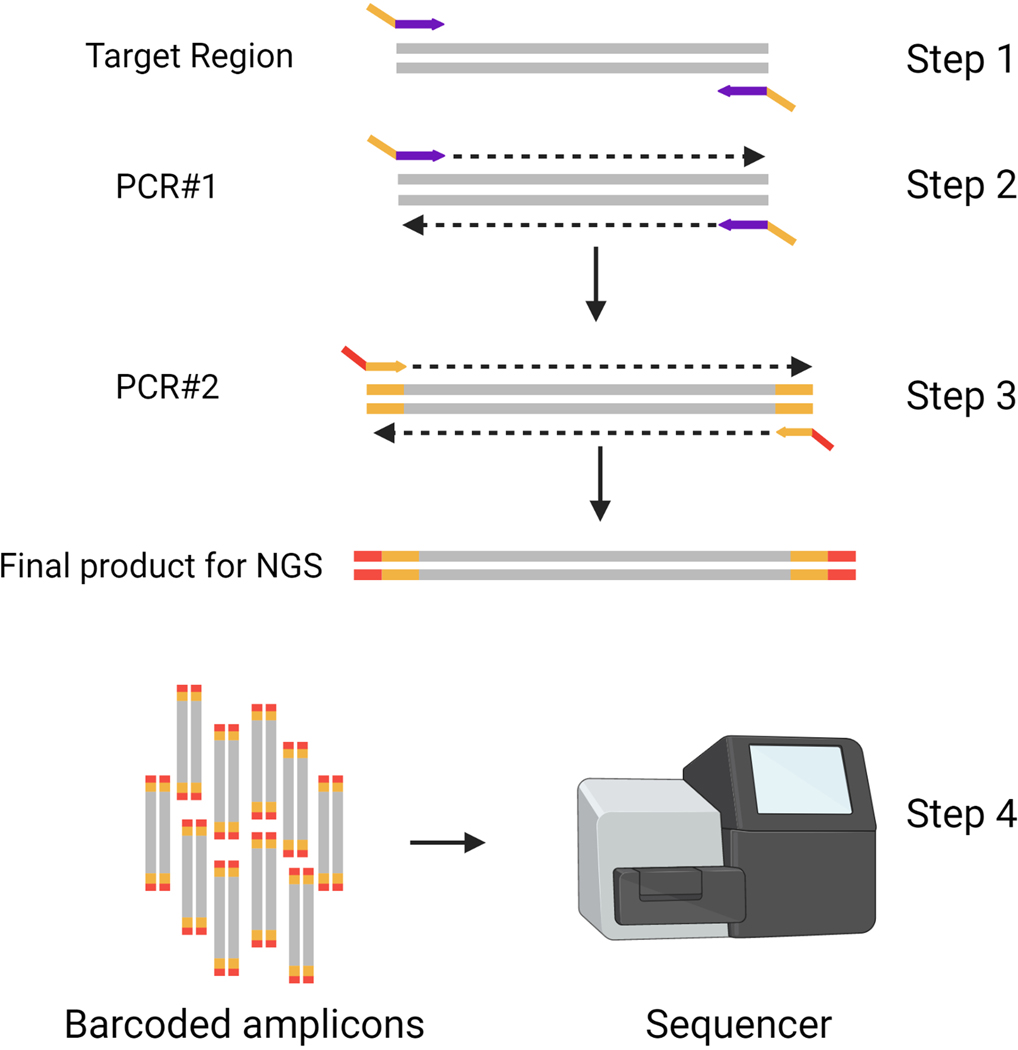
NGS is a massively parallel sequencing technology used for sequencing targeted regions or entire genomes. NGS offers immense scalability and an ultra-high-throughput format with great speed (2,3). The resulting fastq files can be analyzed using different bioinformatic tools. CRIS.py is an NGS analysis program tailored to the interrogation of genome-edited samples, regardless of the genome editing platform. In this protocol, we describe a 2-step PCR process for NGS library preparation. In Step 1, gene-specific primers with partial Illumina adapters are used to amplify the region of interest. In Step 2, the amplicons generated in Step 1 are used as a template for indexing primers containing unique indexes to bind, amplify, and add the remaining Illumina adaptor sequence to the amplicons. This 2-step PCR process allows for the multiplexing of many PCR reactions using the same set of PCR #2 primers. The PCR #2 primers can also be repeatedly used for amplifying and analyzing any number of unique target sites from different projects. There are four key steps in preparing samples for high throughput amplicon sequencing (Figure 1).

Figure 1: Overview of PCR steps for NGS library preparation.

Two rounds of PCR are used to a create an indexed pool of amplicons for targeted deep sequencing. In Steps 1 and 2, primers are designed, and initial amplification is performed. In Step 3, unique indexes are added to the amplicons from PCR #1, before pooling amplicons and sequencing in Step 4. Target region in genomic DNA is shown in grey. Gene-specific primers with partial Illumina adaptors (DS tags) are shown in purple/yellow. Indexing primers are shown in yellow/red.

1. Identify the region to be sequenced and design primers to amplify the target region with appropriate overhangs.

2. Perform PCR #1 on gDNA to amplify the target region and add partial Illumina adaptors to each amplicon.

3. Perform PCR #2 using the PCR #1 reaction as the template and primers containing unique indexes that add a distinctive identifier to each sample and the remaining Illumina adaptor sequence.

4. Sequence the PCR #2 products using an NGS platform.

The unique indexes allow all samples to be pooled together and sequenced in one NGS sequencing run. After NGS is performed, samples are demultiplexed using the unique indexes and reads assigned to each sample. In the Supplemental Materials we have included an Excel file containing our common PCR #2 primer sequences.

3.2. Gene-specific primer design

Design a primer pair to amplify the region of interest for each target for PCR#1. We recommend using PrimerBlast (4) as it also searches for and displays potential off-target amplicons.

1. Design the gene-specific primers for PCR #1 so the total length of the amplicon will be fully sequenced in the NGS run. We recommend sequencing using paired-end 250-bp reads. Design the primer pair such that the total amplicon length is less than 450 bp, with the target-modification site(s) close to the center of the amplicon and the primers binding at least 50 bp away from the cut site. At the end of this section, we will review a few basic primer design strategies for knockout (KO), knock-in (KI), and large deletion projects.

2. Add partial deep sequencing (DS) tags to the 5ʹ end of each primer. These tags serve two purposes: First, they function as a common annealing sequence that the indexed PCR #2 primers can bind to and amplify. Second, they are partial Illumina adaptors and are required for sequencing using Illumina platforms. The Illumina sequencing platform used is determined by the number of reads required. Partial Illumina DS tags are listed below and should be added to the 5ʹ end of the respective gene-specific PCR #1 primer (shown as x’s below).

   1. Forward DS tag:
      5ʹ CTACACGACGCTCTTCCGATCTxxxxxxxxxxxxxxxx 3ʹ
   2. Reverse DS tag:
      5ʹ CAGACGTGTGCTCTTCCGATCTxxxxxxxxxxxxxxxx 3ʹ

The next sections describe primer design for various genome editing strategies.

3.2.1. Primer design for KO and small modification projects

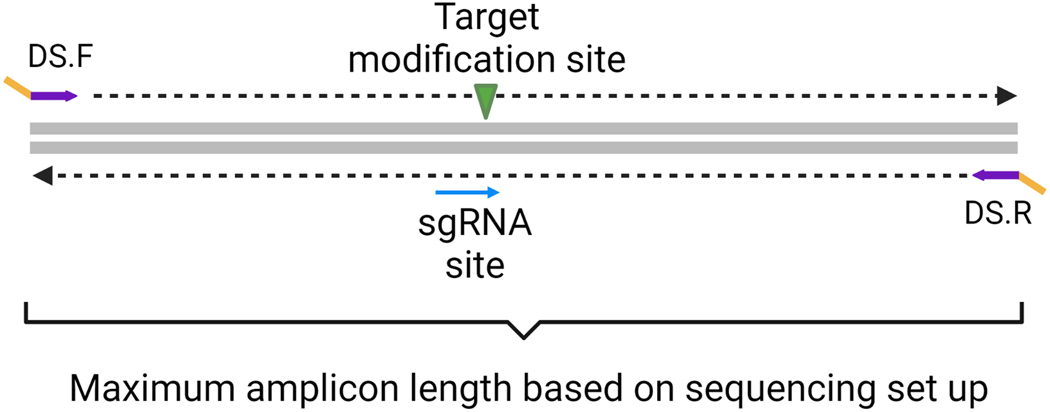
Design a set of primers flanking the modification site (Figure 2). The size of the amplicon must not exceed the size of the paired sequencing read length. The modification site should be close to the center of the amplicon fragment and ideally at least 50bp away from the primer-binding sites.

Figure 2: Basic Primer Design for small insertions and knockout modifications.

Gene-specific forward and reverse primers (purple) with deep sequencing (DS) tags (yellow) are designed flanking the target modification and sgRNA site. The sgRNA site is the location of the 20-nucleotide protospacer and the protospacer adjacent motif (PAM).

3.2.2. Primer design for large deletion projects

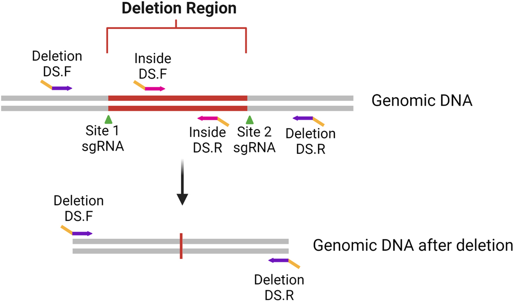
CRISPR-Cas9 may be used to create large deletions encompassing several thousand to mega base pair regions. This is achieved by designing two sgRNAs that flank the region to be deleted. Because each break point of the deletion is known, a primer pair can be designed to amplify and screen for clones containing the targeted deletion. To determine whether the deletion event has occurred, design a forward primer upstream of the 5ʹ-break site and a reverse primer downstream of the 3ʹ-break site (Figure 3). If the deletion was successful, a smaller amplicon size is expected, and can be detected by agarose gel or NGS. If the deletion event did not occur, the remaining sequence is often too large to be amplified with standard techniques or detected by NGS.

Figure 3: Primer Design and PCR strategy for large deletion projects.

Gene-specific deletion primers (purple) with deep sequencing (DS) tags (yellow) are designed flanking the targeted deletion (red region flanked by sgRNA target sites (shown by green arrows). A second set of inside primers (pink) are designed inside the targeted deletion to determine if any untargeted or inverted alleles remain.

Primer design for large deletions is accomplished by first creating a sequence file in which the deletion is modeled. Next, use a primer-design tool to design primers flanking the deletion that are small enough to be fully sequenced by the NGS run parameters. Often, complete-deletion clones are desired in which all alleles for a gene in a cell line contain the specified deletion. To confirm a complete deletion, use the wild-type (WT)/unedited sequence to design a second pair of primers (i.e., inside primers) that bind and amplify in the deletion region. Any clones that are not homozygous for the deletion will contain the sequence and produce an amplicon. Inversion of the intervening sequence between the two cut sites can also occur and would be positive for the inside PCR amplicon.

Because of the multiplexing capabilities of the 2-step PCR method described above, both the deletion-specific and inside amplicons can be pooled, run on a single flow cell with other amplicons, demultiplexed using the unique indexes, and then analyzed using CRIS.py. A complete-deletion clone will have reads for the deletion-specific amplicon and no reads for the inside amplicon because no amplification would have occurred. The amplicons can also be run on an agarose gel, but this becomes labor intensive when screening hundreds of clones for multiple primers sets. Additionally, NGS gives the sequence identity of the deletion allele(s) and further verifies the specificity of the primers.

3.2.3. Primer design for large KI projects

CRISPR-Cas9 technology can knock-in inserts ranging from one to thousands of base pairs. For smaller KIs, where the total amplicon size is within range of NGS for the knock-in allele, use the KO primer design strategy described in section 3.2.1. For larger KIs, junction primers must be designed to detect targeted integration events. Donor templates contain homology arms, which are sequences that are homologous to and flank the targeted genomic region. Donor templates are generally introduced concomitantly with the sgRNA and Cas9 nuclease. Single-stranded donor templates (ssODNs or ssDNAs) have short homology arms (40–200 bp) on each side of the cut and/or modification. Double-stranded DNA (dsDNA) or plasmid donors have longer homology arms (400–800 bp) on each side of the cut and/or modification. Junction (Junc) primers are a set of primers in which one primer binds to the target gDNA outside of the donor homology arm, and another primer binds to a unique site within the sequence to be inserted. Both 5ʹ and 3ʹ- junction primer sets are needed to verify complete targeted integration. It is essential to design junction primers so that they do not bind within either homology arm of the donor. Otherwise, it will not be possible to differentiate targeted integration from random integration of the donor into the genome.

3.2.3.A. Primer design for detecting KI modifications using ssDNA donor templates

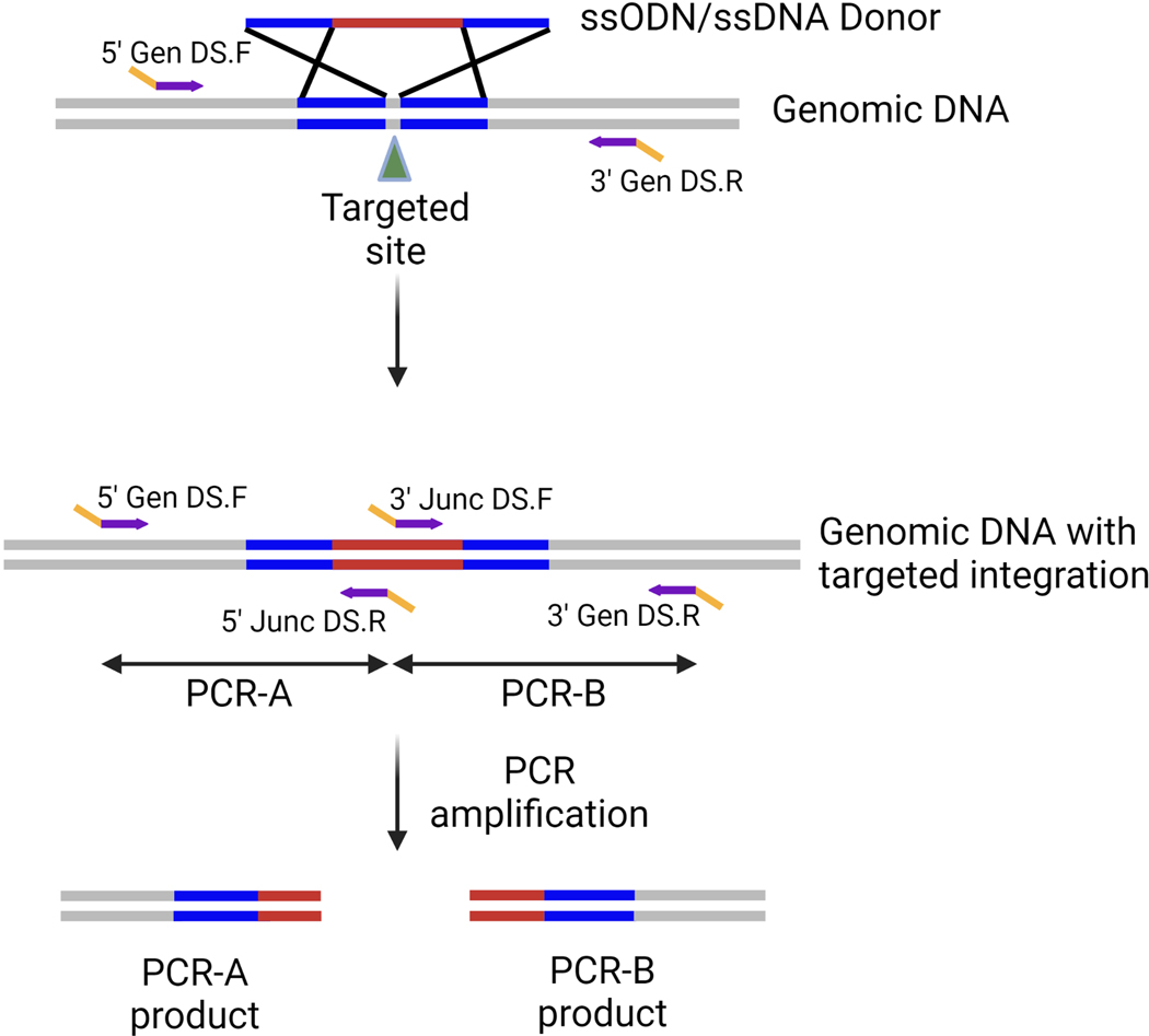
The ssDNA donors used for gene targeting have small homology arms ranging from 40bp to 200bp. The small size allows the design of primers flanking the homology arms and producing an amplicon small enough to be sequenced using NGS. Two sets of primer pairs (PCR-A and PCR-B) are designed using the desired genomic DNA sequence after successful targeted integration as a template. These consist of a 5ʹ junction primer pair (PCR-A) and a 3ʹ junction primer pair (PCR-B) (Figure 4). To determine if clones have any remaining untargeted alleles, perform an “out-out” PCR using the forward primer from PCR-A (5ʹ Gen DS.F) and the reverse primer from PCR-B (3ʹ Gen DS.R).

Figure 4: Primer design and PCR strategy for large ssDNA KI projects.

Two sets of primers are designed to the 5ʹ and 3ʹ regions of the targeted integration event. Each primer set consists of a gene-specific Gen primer (purple region in the Gen primer), which is outside the donor homology arms (shown in blue) and a Junc primer designed to a sequence in the unique sequence to be inserted (purple region in Junc primer). All primers contain DS tags (yellow).

Sequence analysis will determine if the target site remains WT or if an indel has been created by Cas9 cleavage and subsequent repair by NHEJ. Here again, the NGS platform allows the pooling and sequencing of all three amplicons (5ʹ-junction, 3ʹ- junction, and out-out amplicon) for many clones in one sequencing run. Always ensure that you design primers that yield amplicons that are within NGS sequence read length limits.

3.2.3.B. Primer design for KI modifications using plasmid donors

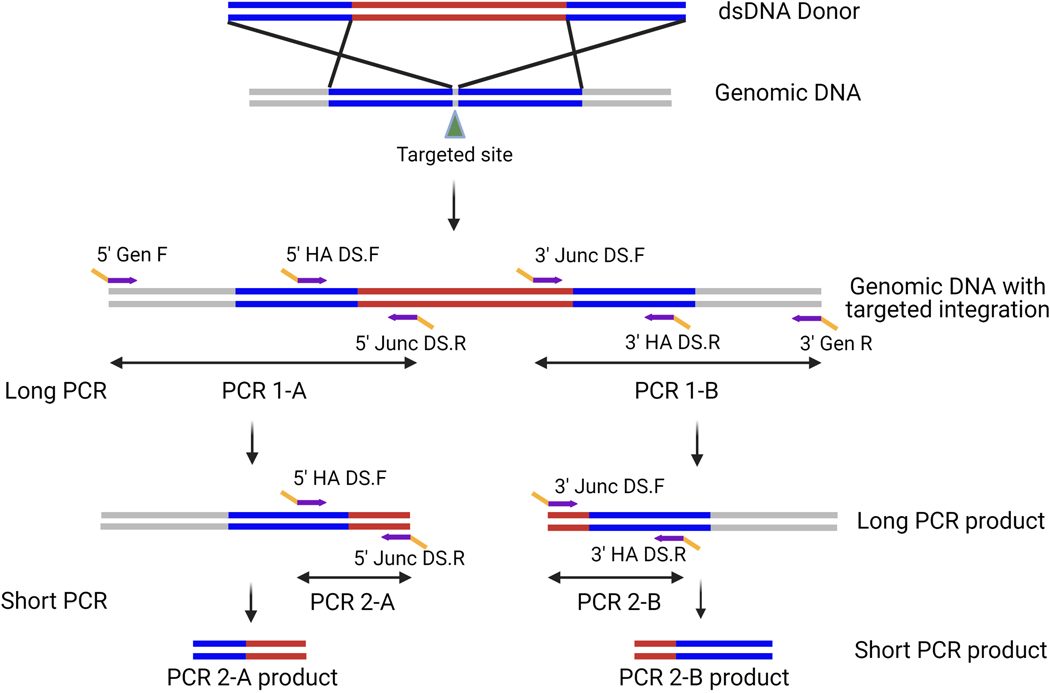
Plasmid dsDNA templates can be used for targeted KI and have larger homology arms. Traditional junction primer sets (described above) that amplify the junctions of integration events made using dsDNA donor templates generally yield amplicons that are larger than current NGS limits (>600 bp). To overcome this limitation, an additional round of nested PCR is required. The initial PCR is set up as described in the previous section with one primer binding in the gDNA outside of each homology arm and the other binding in a unique site of the integrated sequence. Because this amplicon is typically longer than NGS sequence length limits, it is referred to as long-junction PCR (Figure 5). To generate amplicons that are within NGS limits, a nested or short-junction PCR is then performed using the long-junction PCR product as the template. For the short-junction PCR, an additional primer (5ʹ HA DS.F or 3ʹ HA DS.R) is designed that binds in the respective homology arm and is paired with the appropriate Junc DS primer. This amplicon should be within the sequence length limitations of NGS and can be used as the template for indexing PCR #2. When screening recently transfected pools of cells, it is essential to include a donor-only transfected control sample, as the donor plasmid can carry over into the gDNA preparation and result in a false-positive result. If the donor-only transfected sample yields an amplicon after the short-junction PCR, dilute the long-junction PCR product 1:10 and 1:20 and repeat the short-junction PCR. When screening clones, we do not generally see false-positive hits because the plasmid is lost over the many cell divisions required for clonal expansion. However, to ensure a clone is a true-positive hit after being identified by this nested PCR procedure, the long-junction PCR should be repeated on positive clones only and products should be run on a gel as a final quality-control (QC) step. Although this nested PCR process requires an additional round of amplification, it enables the screening of hundreds of clones at the sequence level during one NGS run. We recommended using automation, when possible, to set up PCR reactions in the 96- or 384-well format.

Figure 5: Primer design and PCR strategy for KI projects using dsDNA donor.

Long PCR primers are designed to the 5ʹ and 3ʹ regions of the desired targeted integration event. Each primer set contains a Gen primer designed outside of the homology arm (blue) and a Junc primer designed inside the target KI region (red). Short PCRs primers are designed for nested PCR using the long PCR product as the template to create amplicons that are within the NGS sequence length limits. Short PCR primers consist of a Junc primer, and a HA primer designed within the homology arm. DS tags shown in yellow.

3.3. PCR #1 to amplify the target region

1. Obtain gDNA from all samples by using crude extract (CE) buffer as described in the next step. In general, we find it most efficient to harvest clones from 96-well tissue culture plates without consolidating clones. Additionally, PCR reactions can be minimized in volume to reduce the price per reaction which further brings down the need to make consolidations plates.

2. To harvest gDNA, pellet the cells by centrifugation at >500×g for 5 minutes. Discard the supernatant and add CE buffer. The volume of CE buffer to be added depends on the approximate number of cells in the pellet. Add ~25 μL of CE buffer for every 5000 cells. As it is a crude lysis, amplification may be inhibited if not enough lysis buffer is used. When harvesting from ~80% confluent 96-well plates, we recommend using 25 μL of CE buffer per well. To lyse samples, incubate at 65°C for 15 minutes followed by incubation at 95°C for 5 minutes. Subjecting samples to 95°C inactivates Proteinase K in the buffer preventing further protein degradation.

3. Set up the first-round PCR master mix as shown below (Table 1) using the appropriate primer pair, as described in section 3.2. Gene-specific PCR #1 primer design. To make the master mix, exclude the template (gDNA or long PCR product) and multiply each volume in the Table 1 by the number of samples being tested. The components of the master mix are shown in blue. When possible, use automation to dispense the master mix into 96- or 384-well PCR plates and ensure enough master mix is made to account for the dead volume of the instrument being used.

4. Add 1 μL of gDNA or long PCR product from each sample to the appropriate well containing 9 μL master mix.

5. Run the thermocycler program according to manufacturer’s recommendations. We generally run 30–35 cycles of amplification for PCR #1.

6. Once PCR #1 is complete, check 2 μL of representative samples on an agarose gel to verify the presence of specific bands in appropriate wells. If the bands are present, continue to PCR #2.

Table 1:

Reagents and reaction volumes for PCR#1

Reagent	Volume (μL)
2× MyTaq or Superfi II	5
Forward DS primer (10μM)	0.5
Reverse DS primer (10μM)	0.5
dH20	3
gDNA or long PCR product	1
Total final reaction volume	10

Abbreviations: dH₂O, nuclease-free water; DS, deep sequencing; gDNA, genomic DNA; PCR, polymerase chain reaction

Note: Both the long-junction PCRs and short-junction PCRs are set up as described in this section, with the exception that the long-junction PCR amplicon is used in place of gDNA for the short-junction PCR. Adjust the extension time depending on the length of the amplicon and the polymerase being used.

3.4. PCR #2 to add unique indexes to each sample

1. Set up PCR #2 master mix using the table below (Table 2) as a template. Multiply the volume of each reagent according to the number of samples being tested excluding the PCR #1 template and reverse-indexing primer. The components of the master mix are shown in blue. For each sample, a uniquely indexed forward- and reverse- primer pair is required. We use a combination of 11 forward primers with unique 6 bp indexes combined with 384 reverse primers with unique 10 bp indexes. For a list of functionally validated indexing primers, see Supplementary Tables 1 and 2.

2. Aliquot 8 μL of master mix to the appropriate number of PCR tubes or plates.

3. Add 1 μL of a 10 μM uniquely indexed reverse primer to each tube.

4. Add 1 μL of unpurified PCR #1 reaction to the corresponding tubes/plates containing PCR #2 master mix

5. Run the thermocycler program according to the manufacturer’s recommendations to add indexes. We generally run five cycles of amplification for PCR #2. Keeping the cycle number low will reduce the amplification bias.

6. After completion, pool and submit samples to the NGS facility or vendor for sequencing, demultiplexing, and merging reads.

Table 2:

Reagents and reaction volumes for PCR#2

Reagent	Volume (μL)
2× MyTaq or Superfi II	5
PCR2_Forward Primer (10μM)	0.5
dH20	2.5
Reverse index primer (10μM)	1
PCR #1 product	1
Total final reaction volume	10

Abbreviations: dH₂O, nuclease-free water; PCR, polymerase chain reaction

Note: To increase sequence diversity, we recommend adding at least 10% PhiX Control v3 to the indexed amplicon pool. Additionally, purify the amplicon to reduce primer dimer contamination. Further QC measures (e.g., Bioanalyzer or q-PCR) may be needed to determine the appropriate amount of library to load for proper clustering.

3.5. Using CRIS.py to analyze NGS data

CRIS.py is an analysis program that runs in a Python environment. CRIS.py enables users to analyze thousands of NGS-generated output files quickly and efficiently. The script also lets users query and quantify multiple editing events concurrently. In this section, we will discuss installation guidelines and how to modify the script to analyze multiple genome-editing outcomes in cell pools and clones.

3.5.1. Installing Python and CRIS.py

CRIS.py utilizes Python 2.7 or above and the pandas module. Python can easily be installed using the Anaconda link shown here. https://www.anaconda.com/products/individual

CRIS.py can be downloaded from the following link at GitHub.

https://github.com/patrickc01/CRIS.py

A detailed tutorial video on how to use CRIS.py is available at the link below.

https://s.stjude.org/video/player.html?videoId=6000021936001

3.5.2. Setting up a folder with the CRIS.py script and NGS data

The fastq files generated from an NGS run and the corresponding CRIS.py programs should all be copied to the same directory.

3.5.3. CRIS.py program layout

Figure 6 shows an example CRIS.py program with user-defined inputs in single quotation marks. The example CRIS.py program shown in Figure 6 has been referenced from GitHub (5) and modified for illustration.

Figure 6: Example of a CRIS.py program.

CRIS.py contains several editable variables that enable the program to be customized to the desired genome-editing outcome. See “Variables of the CRIS.py program, section 3.5.4” for variable definitions. Variables to be modified by the user are shown between quotation marks (‘ ’).

3.5.4. Variables of the CRIS.py program

A key feature of the CRIS.py program is that it enables users to change the script to suit their experimental needs. Script changes can be made at any time, and data can be analyzed accordingly. CRIS.py allows the parameters listed below to be changed in the script. User inputs should be entered between the quotation marks (Figure. 6). All user- input variables can be entered as uppercase or lowercase letters. The letters below correspond to the lettering in Figure 6.

1. “ID” specifies the name of the output file that will be generated. Each program should be uniquely named.

2. “ref_seq” defines the reference input sequence. The input sequence is the target-specific amplicon sequence obtained using the PCR#1 primers and excludes the DS tags.

3. “seq_start” is an approximately 10 to14 bp sequence downstream of the PCR #1 forward primer and upstream of the modification site. This length is generally long enough to be unique in the pool of amplicons and short enough to reduce the loss of reads due to sequencing errors.

4. “seq_end” is an approximately 10 to14 bp sequence upstream of the PCR #2 reverse primer and downstream of the target site. This length is generally long enough to be unique in the pool of amplicons and short enough to reduce the loss of reads due to sequencing errors.

5. “fastq_files” is the location and name of the fastq files to be analyzed. If the well position of a sample to be analyzed is known, it can be inputted. Otherwise, entering *.fastq will query all the fastq files in the directory.

6. “test_list” contains the list of sequences to be queried. The program analyzes reads for all sequences entered in the test list and reports them in a column with the corresponding name. These sequences can include full-length sgRNA- binding sites, desired HDR edits, specific indels, or even single nucleotide polymorphisms (SNPs). The test_list sequences should be between the seq_start and seq_end, and all test_sequences (G), seq_start and seq_end sequences must be copied from the top strand only. For example, all sequences should be found on the R1 sequence in the fastq file, as the analysis is strand specific.

3.5.5. How does CRIS.py work?

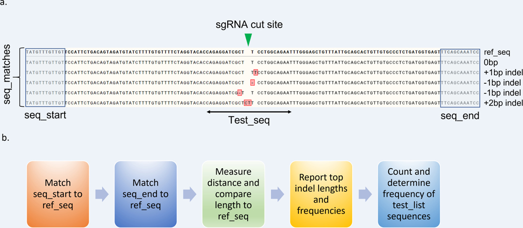
CRIS.py uses input variables to search and find reads within fastq files. The process CRIS.py uses to analyze fastq files is described below and in Figure 7a and 7b.

Figure 7: Overview of CRIS.py analysis pipeline.

(a) An example reference sequence is shown labeled with CRIS.py program variables. CRISPR-Cas9–induced indels from the .txt file were aligned to the reference sequence and high-lighted in red. Indel sizes are manually labeled on the side for reference. (b) Process flow for CRIS.py analysis.

1. Two flanking sequences (seq_start and seq_end) are matched to the ref_seq to determine the distance between the two sequences and establish a reference for the expected WT sequence length.

2. All reads in a fastq file are analyzed for both the seq_start and seq_end. If both sequences are found, they are counted (termed a “seq_match”). For every seq_match, CRIS.py calculates the length from seq_start to seq_end and compares the length to the WT reference sequence length established in Step 1.

3. An amplicon that has no indel and matches the WT length is reported as a 0 bp indel. Amplicons that differ from the WT length are reported with their respective indels sizes. Deletions are reported as a negative number.

4. A net zero indel is also reported as 0 bp indel. For example, if a −2 bp and a +2 bp indel occur in the same amplicon, the net indel size is reported as 0 bp.

5. Indel frequencies are calculated by combining the total number of reads for each indel size and dividing that by the total number of seq_matches.

6. CRIS.py determines the frequency of all user-defined sequences in the test_list (termed test_seq) by summing the number of times a test_seq occurs divided by the total number of seq_matches.

7. SNP_test is calculated as part of the QC for the CRIS.py script and sequencing data. It represents a ratio between the total number of times the seq_start and seq_end sequences are counted in each fastq file. The ratio should be ~1. If a SNP occurs in either the seq_start or seq_end region, the SNP_test value varies depending on how many alleles have the SNP. Large indels resulting in the loss of seq_start or seq_end will also affect the SNP_test score. Additionally, poor-quality NGS data can result in an aberrant SNP_test.

8. SNPs can be present at both the seq_start and seq_end in one or more alleles. This would cause the SNP ratio to remain approximately the same. To test this potential scenario, CRIS.py includes an additional QC step that is reported as raw_wt_counter. This value represents the ratio of the number of reads found for the first test_seq of the test_list within the raw fastq file for a given index and the number of reads for the same sequence found in seq_match sequences. It should be ~1 for a WT control sample. The raw_wt_counter will be 0 if the first test_seq is not present in the samples. For example, if the sgRNA target site is the first test_seq and the sample is a complete KO clone, the test_seq will not be found in the raw fastq file and the raw_wt_counter will be 0.

Note: It is important to align the reads to the reference sequence to know the exact indels present in a sample.

3.6. Set up and analysis of CRIS.py-generated data for various editing scenarios

Once the desired variables have been entered, the CRIS.py program is run. This generates a .csv file and a .txt file. The .csv file is a master summary file that provides (1) the total read count; (2) the read counts and frequencies of all sequences in the test_list; (3) the read counts, frequencies, and lengths of the top indels; and (4) the QC checks. The .txt file lists the test variables and provides the sequence identities and read counts of the most common reads.

The analysis of data generated by CRIS.py differs based on the scope of the genome editing project. This section describes the set up and analysis of CRIS.py data for various types of editing outcomes.

3.6.1. KO projects

3.6.1.1. Setting up CRIS.py script for a KO project

This section describes the process of entering variables in the CRIS.py script for analyzing a KO project. All variables should be entered between the quotation marks, as shown in Figure 6.

1. Enter “ID” for your project.

2. Enter the “ref_seq” of your target PCR, as shown in Figure 8a and below.

3. Enter “seq_start” and “seq_end” sequences.

4. Enter test_seqs of interest. Figure 8a shows the sgRNA target site (i.e., 20 nucleotide protospacer plus 3 bp Protospacer Adjacent Motif [PAM]) as the test_list sequence. The name of the sgRNA(s) used should be added within the str(‘ ’) and the sequence of the corresponding sgRNA target site should be added into str.upper(‘ ’).

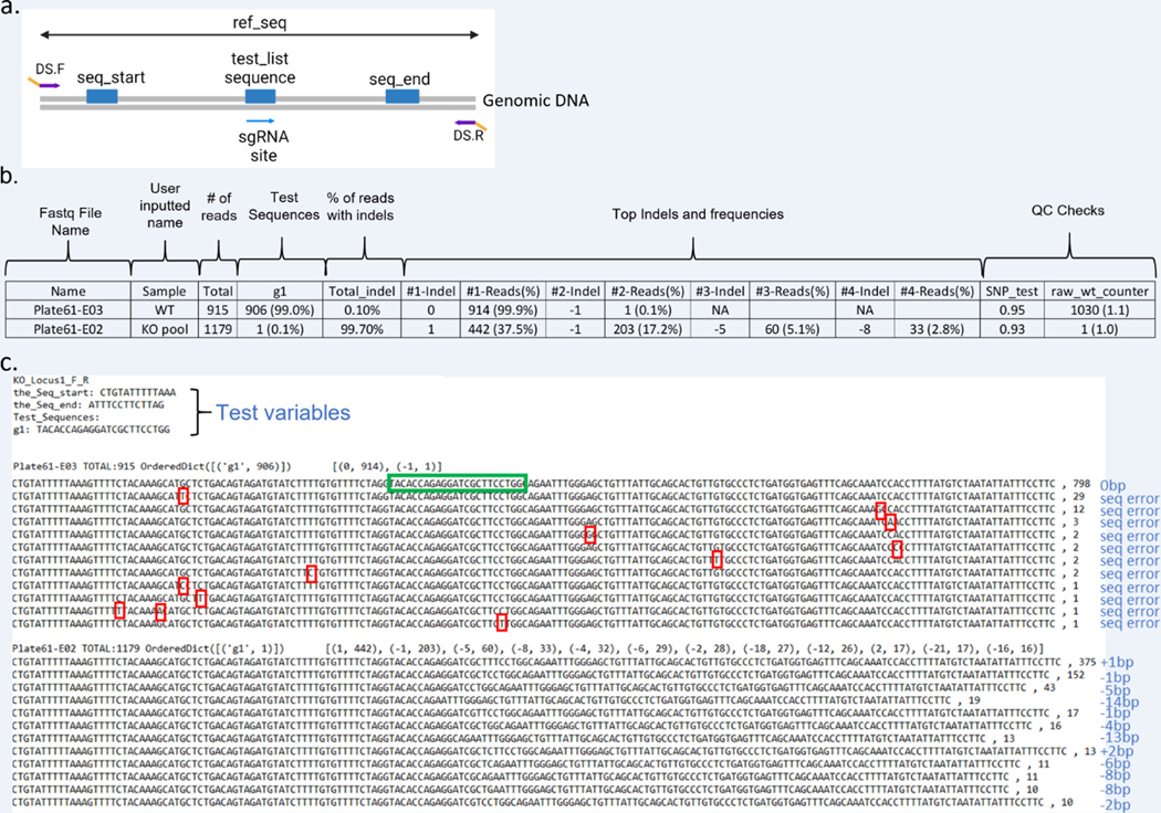
Figure 8: Set up and analysis of CRIS.py data for a KO project.

(a) Representation of the region of interest and CRIS.py variables in a KO project. The primers to amplify the targeted region are DS.F and DS.R. The gene-specific portion of the primers is shown in purple and the DS tags in yellow. The seq_start, seq_end and test_list sequences to be included in the CRIS.py script are shown as blue boxes. (b) Example data from a .csv file generated by CRIS.py analysis of a KO cell pool with features high-lighted. (c) Example data from a .txt file generated for CRIS.py-analyzed KO pool samples. The sgRNA (g1) sequence is shown in a green box. Indels and sequencing errors in the sample are labeled in blue text. Sequencing errors (seq error) in the WT sample are marked by red boxes.

3.6.1.2. Analyzing and interpreting data for a KO project

3.6.1.2.A. Interpreting the output .csv file

Figure 8b represents the output .csv file from the NGS data for a KO project.

1. The first column “Name” specifies the fastq file name and plate location of the sample based on the unique indexes added during the NGS library creation.

2. The “Sample” column is left blank intentionally, so that the user can manually assign sample names to the corresponding fastq file name. In this example, we have assigned the labels “WT” and “KO pool.”

3. The total number of reads obtained for each sample is shown in the “Total” column.

4. All test_seq counts and frequencies will be reported in the columns between “Total” and “Total_indel.” In this example, only one test_seq was queried (g1). For a KO project, the test_seq is generally the sgRNA target site including the PAM. A highly active sgRNA will result in large percentages of reads with indels at the cut site and thus low numbers of reads with the exact match to the sgRNA-specific test_seq. The lower the percentage of exact matches to the sgRNA target site test_seq, the higher the sgRNA activity. In this example, the results indicate that 0.1% of the reads in the KO pool sample have an exact match to the tested sgRNA target compared to 99% of the reads in the WT sample. This indicates a highly active sgRNA.

5. The column “Total_indel” shows the total indel frequency for each sample. In this example, the WT sample has approximately 0.1% Total_indel. In some cases, the Total_indel for negative-control samples may be slightly higher due to sequencing or amplification errors. It is important to run a WT control sample to determine and account for amplicon specific sequencing errors. For example, some amplicons contain long stretches of repetitive sequence that, cause sequencing and/or amplification issues. Sample g1 reports 99.7% “Total_indel,” which indicates that 99.7% of the reads in this sample do not have the WT sequence length and thus contain indels. The “Total_indel” is calculated by subtracting the percentage of 0 bp indels from 100%.

6. CRIS.py reports the top 8 indels by frequency. The top 4 indels are shown in the examples for simplicity. Indel sizes relative to the ref_seq are reported in columns labeled “#-indel.” An indel length of “0” is reported for reads with the same length as the ref_seq (WT length).

7. Each “#-indel” column has a “% Reads” column adjacent to it. This column represents the total number of reads and percentage of reads for that indel length.

8. For unedited or WT samples, the “#1-Reads (%)” value and the first test_seq (g1 in the above example) should theoretically be the same. However, the “#1-Reads (%)” value is usually higher and does not match the first test_seq because the values reported in the test_seq column are calculated based on the exact match to the test_seq sequence, whereas the “#1-Reads (%)” value is reported based on the length of the indel. The longer the test_seq is (in base pairs), the more chance for sequencing error and disparity between these two columns.

9. A 0 bp indel indicates that the amplicon is of WT length. NHEJ events can also result in nucleotide transitions or transversions, which would not affect the amplicon length and would also be reported as 0bp. This also contributes to disparity between the “g1” test_seq and “#1-Reads(%)” values for the WT sample (discussed above). This technical disparity is generally small and should not change the overall interpretation or clone choice.

10. All indels of the same length are binned together and reported in the top #-Indels columns. That is, more than one distinct indel can be binned and counted together based on length. To determine if unique indels of the same length have occurred in a clonal sample, you can review the .txt file.

11. Columns “SNP_test” and “raw_wt_counter” provide QC measures for each sample. See section 3.5.5 (7 and 8) for more details.

3.6.1.2.B. Interpreting the output .txt file

The second output file generated by CRIS.py is a .txt file (Figure 8c). The .txt file contains the test variables that the user entered into the program. This is followed by the sequence reads for each of the samples. The samples can be identified by the well and plate location corresponding to a unique barcode.

1. For each sample, all indel sizes and their corresponding number of reads are presented in brackets next to the sample/well identifier name.

2. For each sample, the most highly represented sequences are listed with the total number of reads for each unique sequence. Sequence reads must match exactly to be binned together. Although the WT sample in “Plate61-E03” contains reads of the same length, they are binned separately because of errors occurring during PCR amplification or sequencing error (See Figure 8c, red boxes). All these reads would be reported as 0 bp indels because their length matches the ref_seq.

3. The sequences can be used to compare the reads obtained for various samples and aligned with the ref_seq to determine the sequence identity.

4. The .txt file can also be used to quickly identify samples in which editing has occurred by looking for a difference in the length of sequence reads as in the “Plate61-E02” sample in Figure 8c. The differences in length are caused by NHEJ-induced indels.

3.6.2. Small modification projects

3.6.2.1. Setting up CRIS.py for small modification projects

This section describes the steps to set up CRIS.py for analyzing small modification projects. All variables should be entered between the quotation marks, as shown in Figure 6.

1. Enter the sequences of variables, as shown in Figure 9a.

2. Enter the test_list sequences that have been marked in Figure 9a. For a small modification project, you may enter multiple sequences in the “test_list”. As a default, include the sgRNA target site. The name of the sgRNA(s) used should be added within the str(‘ ’) and the sequence of the corresponding sgRNA target site should be added into str.upper(‘ ’).

3. The number of sequences in the “test_list” depends on the design strategy of the project. In the example below, an ssODN was designed to create a targeted point mutation (red X). However, because a single base pair difference between the WT sequence and the edited sequence may not be enough to prevent recutting by Cas9 and subsequent repair by NHEJ after the desired integration event has occurred, we recommend incorporated a silent blocking modification (purple X). Because the goal of the project is to make the desired point mutation with or without the blocking modification, clones with either the modification only or the small modification and the blocking modification would be useful. CRIS.py facilitates the interrogation of multiple test_seqs. In this example, we recommend listing the modification only (Mod_only), the modification + blocking (Mod_Block), and the blocking only (Block_only) as test_seqs as shown in Figure 9a.

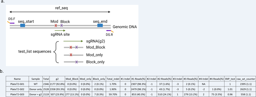
Figure 9: Set up and analysis of CRIS.py data for a small modification project.

(a) Example of a targeted editing site and variables used in CRIS.py for a small modification project. The gene-specific portion of the primers is shown in purple and the DS tags in yellow. The variables are shown as blue boxes, and test_list sequences represented are shown below. (b) Example of the .csv output file of CRIS.py analysis. The top 4 indels are shown for representation purposes only.

3.6.2.2. Interpreting the data in the output .csv file for a small modification project

CRIS.py analyzes and measures HDR rates in pools of cells. The desired HDR events are entered as test_seqs within the test_list portion of the Python script in the same manner as above. An example of CRIS.py analysis for small HDR events is shown below and in Figure 9b.

1. Columns labeled “g2,” “Block_Mod,” “Mod_only,” and “Block_only” are the names of the test_seqs. CRIS.py allows the user to query any combination of edits within an amplicon. In this example, we are analyzing for the sgRNA target site, the desired small modification with or without the blocking modification, and for the blocking modification alone.

2. Sample “Donor only” is a control in which cells have been transfected with the donor ssODN only without the sgRNA or Cas9. The percentage of test_list sequences for this sample should be ~0, except for the “g2” test_seq as the gRNA site should be intact if no cutting has occurred.

3. Sample “Donor + g2” shows that 23.9% of the reads have the “g2” test_seq, and the WT sample shows that 92.8% of the reads have the “g2” test_seq. The WT sample will typically have an exact match to the 23 bp target site less than 100%. This is because to be counted as a match, every base pair of the test_seq must match the sequence read exactly. Sequencing errors at any position within the test_seq will result in the read being excluded from the count. For this reason, it is important to limit the length of the test_seq and/or weigh the impact of having a long test_seq: the longer the test_seq, the lower the number of reads with an exact match to the test_seq.

4. The percentages of the test_seqs report the percentage of reads in the sample that match exactly to the input test sequences. The sample “Donor + g2” has 13.1% of reads matching the Mod_Block sequence. The “WT” and “Donor only” samples have 0% of the reads matching the Mod_Block sequence. Therefore, ~13% of the alleles in the pool contain the Mod_Block sequence.

5. The “Total_indel” column reports the total number of reads that do not have the WT length (59.7% in treated sample and 1.7% in WT sample). The WT control should have very low reported rates of indels, and the top non–0-bp indel sizes are generally ± 1 bp resulting from sequencing error.

6. If you are knocking in a small insert that will yield an amplicon of different length to the ref_seq, you will see the corresponding indel length reported by frequency as with other indels. It is important to note that there may be PCR bias and a corresponding underrepresentation of the KI indel length. Amplicons that differ in size, even by 10–20 bp, will be differentially amplified with the smaller amplicon being amplified preferentially. Larger size differences will produce a bigger bias towards the smaller amplicon. This PCR bias will also be present in the frequency of test_seqs reported for small KI projects that yield amplicons that differ in length from the ref_seq.

7. CRIS.py reports the top 8 indels by frequency. The top 4 indels are shown in the examples for simplicity. Indel sizes, relative to the ref_seq, are reported in columns labeled “#-indel.” An indel length of “0” is reported for reads with the same length as the ref_seq (WT length).

8. Each “#-indel” column has a “% Reads” column adjacent to it. This column represents the total number of reads and percentage of reads for that indel

9. The SNP_test and “raw_wt_counter” should be ~1, as in the other examples if the first test_seq (perfect deletion) is found in the seq_match.

3.6.3. Deletion projects

3.6.3.1. Setting up CRIS.py for a deletion project

This section describes the process of entering variables in the CRIS.py script to analyze a deletion project.

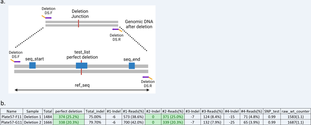
1. Enter variables, as shown in Figure 10a. The “ref_seq” for a deletion project is the expected genomic sequence after the deletion event and assuming precise rejoining of the sgRNA cut sites.

2. Select the region at the deletion site from the sequence obtained after successful deletion and use it as a test_seq in the test_list. This region can be named “perfect deletion” and should be ~14 to 20 bp long.

Figure 10: Set up and analysis of CRIS.py data for a deletion project.

(a) Example of a deletion product and the variables used in the CRIS.py program for deletion analysis. The red line indicates the joining after the deletion event occurred. The gene specific portion of the primers is shown in purple, and the DS tags in yellow. The variables in the script are shown as blue boxes. (b) Example of a .csv output file for a deletion project analysis by CRIS.py. Two representative deletion pool samples are shown.

3.6.3.2. Interpreting the data in a .csv file of a deletion project

1. The test sequence in a typical deletion project test_list, is the perfect deletion sequence (Figure 10a).

2. In Figure 10b, the column “perfect deletion” represents the percentage of reads in the sample that matches the sequence obtained if a perfect deletion event has occurred. Deletion 1 and Deletion 2 samples have 25.2% and 20.3% of the reads, respectively, that have the perfect deletion sequence.

3. For deletion projects, a 0 bp indel also represents the reads with a perfect deletion, as the ref_seq length is the expected length after a perfect rejoining of the sgRNA cut sites. If a precise deletion is not needed for the downstream application, reads with other indels may also be useful.

4. As previously described, there may be small differences between the 0 bp indel and the “perfect deletion” test_seq frequencies because of the difference in how each is calculated: the “perfect deletion” column will report back exact matches to the test_seq whereas the 0bp indel (#2-indel in Figure 10b) reports the frequency of the reads with the ref_seq length regardless of sequence.

5. The SNP_test and “raw_wt_counter” should be ~1, as in the other examples if the first test_seq (perfect deletion) is found in the seq_match.

Notes: Writing a CRIS.py program for the inside PCR (see Figure 3) and including the inside PCR amplicon in the NGS run can be done to determine the zygosity of clones in a deletion project. If a given sample has reads for both the deletion PCR and the inside PCR, that indicates the clone is heterozygous for the deletion. This can also be confirmed by analyzing the PCR products by gel electrophoresis. A clone with no remaining unedited alleles deleted clone would have no sequence reads for the inside PCR.

3.6.4. Large KI projects

3.6.4.1. Setting up CRIS.py for a large KI project

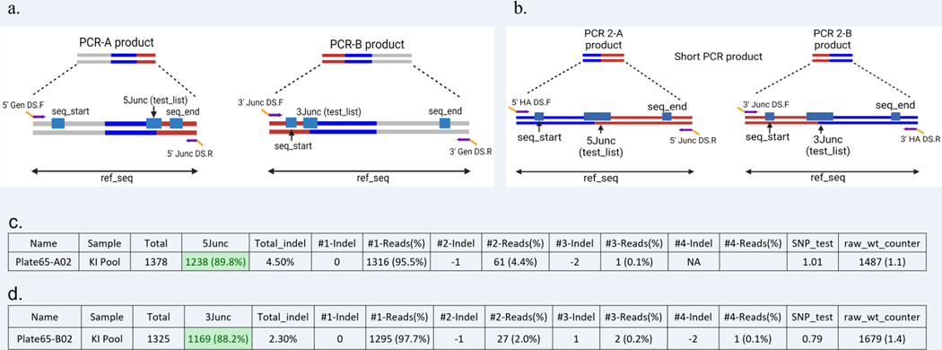
As described in the Primer Design for Large KI projects (section 3.2.3), the analysis for large KI projects involves multiple PCR amplicons (Figures 4 and 5). Thus, there will be multiple CRIS.py programs: one for each amplicon. The 3 key analysis scripts for a KI project are (1) FR, (2) 5Junc, and (3) 3Junc programs. The 5Junc and 3Junc programs are used to detect the integration of the large KI at the 5ʹ and 3ʹ ends, respectively. The FR program uses primers that are designed in the gDNA region flanking the targeted integration site; this program is used to determine if any unedited or indel alleles remain. This section describes the process of entering variables in the CRIS.py scripts for analyzing a large KI project.

1. Enter variables for the 5Junc and 3Junc CRIS.py programs, as shown in Figure 11a (for ssDNA KI) or Figure 11b (for plasmid dsDNA donor KI).

2. If you are analyzing clones and want to know if they are heterozygous or homozygous for the KI, perform a PCR using the Gen DS.F/Gen DS.R primer set for an ssDNA KI and using the HA DS.F/HA DS.R primer set for a dsDNA KI project. Write a CRIS.py script using the WT genome sequence as the “ref_seq” (see section 3.6.1. KO project and Figure 8a).

Figure 11: Set up and analysis of CRIS.py data for a large KI project.

Example of the KI products obtained by Junction PCRs and the variables used in the CRIS.py program for a KI project using ssODN/ssDNA (a) or dsDNA (b). The PCR products shown in figures a and b can be referenced to the final PCR products in figures 4 and 5 respectively. The gene-specific portion of the primers is shown in purple and the DS tags in yellow. The variables in the script are shown as blue boxes. (c) Example of the .csv output file for 5junc PCR analysis by CRIS.py. (d) Example of the .csv output file for 3junc PCR analysis by CRIS.py.

3.6.4.2. Interpreting the data in a .csv files of a KI project

1. A separate .csv file will be generated for each CRIS.py program/amplicon: one for each junction program (5Junc and 3Junc).

2. The respective “5Junc” and “3Junc” test_seq columns will report the percentage of reads in the samples that have the precise junction.

3. In example Figure 11c, the KI pool sample has 89.8% of the reads with the 5Junc test_seq.

4. In example Figure 11d, the KI pool sample has 88.2% of the reads with the 3Junc test_seq.

5. The total indels for the 5Junc program and 3Junc program are 4.5% and 2.3%, respectively. This indicates that the remaining 95.5% and 97.7% of the sequences match the ref_seq length, which is reported in the “#1-Reads (%)” column. In this example, ref_seq is the sequence with the precisely targeted integration incorporated at either the 5ʹ or 3ʹ junction.

Notes: Depending on the size of the insert, it is likely that the out-out primer sets will yield no reads in homozygous KI clones as the resulting amplicon size would be beyond the read length limit for NGS. If a clone is heterozygous for the KI, NGS data is obtained for both the junction PCR sets as well as the out-out primer PCR sets. The modified allele(s) would be positive for the junction PCRs and the nonintegrated allele(s) would be positive for the out-out PCR.

3.6.5. Interpreting the CRIS.py .csv output file for clonal data

The above examples show how to use CRIS.py and interpret the output files to determine editing frequencies within a pool of edited cells. CRIS.py is also highly useful for screening and identifying desired edited clones. The output .csv file is searchable and sortable, allowing for quick and efficient clone identification. In general, the same program written for determining the rates of editing in the pool can be used for identifying correctly edited clones. However, the analysis is different.

Below we discuss how to interpret the output .csv file (Figure 12) when screening for clones with a desired point-mutation modification. The example shown below is the single cell screening data for the same point mutation project described in section 3.6.2.

Figure 12: Analysis of CRIS.py data for screening single-cell clones.

Example of a .csv output file for screening single-cell derived clones for a point mutation project. The different clone types identified in the screen are labeled in the sample column. Clones with low read counts are highlighted in red. Homozygous clones (Hom Clone) are highlighted in green. Heterozygous clones (Clean Het) with the desired modification (Mod_Block) on one allele and the WT sequence on the other allele are highlighted in blue. Heterozygous clones with indels (Het Clone + Indels) on one allele and the desired modification (Mod_Block) on the other allele are shown in yellow. Clones with all out-of-frame indels (KO) are highlighted in purple. The top 2 indels are shown for representation purposes only.

1. Finding a correctly edited KI clone can require screening hundreds of individual clones. To quickly narrow the candidates that have the desired modification, sort the .csv file by “%Mod_Block.” Because the column labeled “Mod_Block” lists both the number and percentage of reads in each clone with the given test_seq, you cannot use this column for sorting. The frequency of all test_seqs is listed separately in the corresponding column with a percent sign “%” before the test_seq name. These columns are listed after the raw_wt_counter to facilitate sorting of the .csv file on a given variable. In the example in Figure 12, only “%Mod_Block” is shown for simplicity.

2. Clones with low reads may have fewer cells in the harvested well and may have skewed allelic frequencies. In general, we recommend picking clones with at least 100 reads in the “Total” column.

3. For a point mutation project, you should identify clones with the desired modification and, ensure that there are no indels in the desired clone by examining the “Total_indel” column. The “Total_indel” should be ~0, the “#1-indel” should be 0 bp, and the “%Mod_Block” should be ~100% for a homozygously edited clone (Figure 12, green rows). A diploid clone, in which one allele contains the desired edit and the other contains an NHEJ event, should have a “%Mod_Block” of ~50%, a “Total_indel” of ~50%, and the top two indels would be the 0 bp indel (KI) and the indel length of the NHEJ allele.

4. A clean heterozygously edited clone (Figure 12, blue rows) has the desired modification on one allele and remains WT on the other allele. In this case, “Total_indel” remains ~ 0%, but the “%Mod_Block” column will have ~ 50%, and the “%g2” column (not shown) will have ~50%. This is because only one allele has the desired modification; and the other allele has a WT sequence.

5. Indel frequencies (#-Reads(%)) with low percentages can generally be attributed to sequencing errors and typically account for less than 3% of the reads per specific indel. However, before choosing a clone for expansion, the user should align the sequence reads from the .txt file with the desired sequence to confirm that no indels align with the sgRNA site, which might be indicative of a nuclease-induced indel.

6. It is often possible to identify KO clones when creating a targeted KI clone if the resulting indels lead to a premature stop codon. KO clones will have only out-of-frame indels in the “#-Reads(%)” columns with adequate read counts and near 100% in the “Total_indel” column (Figure 12, purple row). Note that the KO clone in Figure 12 contained the desired “Mod_Block” modification. However, the top two indels were not 0 bp, which indicates that additional insertions or deletions have occurred on the edited allele.

7. The SNP_test and the raw_wt_counter columns are reported for each clone. The SNP_test should always be considered, but the raw_wt_counter will be 0 if the first test sequence is not found in the clone.

8. Align the sequence data of the selected clones in the .txt file with the reference file to confirm the desired edit and precise knock-in of the sequence.

4. Trouble shooting and recommendations

4.1. Unable to amplify the target regions

1. Check the concentration of DNA in the sample. Too little or too much gDNA can inhibit amplification.

2. Optimize PCR conditions for a given amplicon.

3. Check GC content of the desired amplicon. If it is higher than 65%, we recommend using an additive (e.g., DMSO, betaine or GC enhancer) to improve amplification rates for GC-rich amplicons.

4.2. Low read count

1. Check the QC metrics of the NGS quality via the Illumina software.

2. Check amplicon size and relative quantity on an agarose gel.

3. To increase sequence diversity, it is recommended to add at least 10% PhiX Control v3 (Illumina Cat# FC-110–3001) to the indexed amplicon pool. Low sequence diversity can impair correct base calling on the Illumina sequencer.

4. Reduce primer dimer contamination by amplicon purification. This will reduce primer dimers which can consume reads in the sequencing run.

4.3. No data in .csv file

1. Check the CRIS.py program for any errors.

2. Verify that the script is being executed in the same directory where the fastq files are located.

3. Check if each test_list sequence is separated by a comma (,).

4. Verify that the sample location specified in the variable “fastq_files” is correct.

5. The most common errors are the “ref_seq”, “seq_start”, “seq_end” and sequences in the “test_list”. Check each one to ensure the correct sequences from top strand have been provided.

6. Check the size of the final amplicon to ensure it is within the NGS run length limits.

7. Move the “seq_start” and “seq_end” sequences, as one or both may be landing on a SNP or a repetitive region, which would result in no reads.

8. Confirm the amplification of the PCR product by gel electrophoresis.

9. Download and test analysis using data from the CRIS.py GitHub site.

4.4. SNP_test ratio is not near 1.0

1. A SNP may be present in the seq_start and/or seq_end in one or more alleles. Pick a different seq_start and/or seq_end sequence inside the primer sequences and rerun.

4.5. The raw_wt_counter is not as expected

1. Check to see if your first test_seq should be found in the raw reads or seq_matches. The raw_wt_counter value would be “~0” for total KO clones or deletion clones if the first test_seq is the sgRNA target site that was used for the editing event. This is because the test_seq will not be found in the fastq file if editing has occurred.

4.6. Total indel value is high in the WT/negative control

1. Check if there is a repetitive stretch inside the seq_start and/or seq_end sites. If one is present, move the seq_start and/or seq_end sequences to avoid the region and rerun the program.

Summary

NGS is a powerful tool for determining genome-editing outcomes. However, it is not without limitations, including read-length limits, the inability to detect larger chromosomal aberrations, and PCR bias for smaller amplicons. Nevertheless, targeted NGS enables high-throughput screening because many individual samples can be indexed, pooled, sequenced, and the resulting data demultiplexed to provide the sequence identity of edited samples. The large amounts of data generated by NGS can be efficiently analyzed using CRIS.py, which allows users to simultaneously analyze many clones at great speed and with high accuracy. In this chapter, we detailed NGS library preparation, primer design, and setup and analysis of CRIS.py for a variety of genome editing scenarios. The flexibility in modifying the CRIS.py script, per the user’s needs, makes it a great tool for analyzing any number of editing outcomes in cell pools, single clones, and animal models. The output files generated by CRIS.py are editable and in a format that enables users to quickly search, rank, and identify clones of interest. The ease of running CRIS.py locally on most computers and the speed of analysis makes it a powerful tool for analyzing NGS data for genome editing outcomes.