A two-stage adaptive clinical trial design with data-driven subgroup identification at interim analysis

Abstract

In this paper, we consider randomized controlled clinical trials comparing two treatments in efficacy assessment using a time to event outcome. We assume a relatively small number of candidate biomarkers available in the beginning of the trial, which may help define an efficacy subgroup which shows differential treatment effect. The efficacy subgroup is to be defined by one or two biomarkers and cut-offs that are unknown to the investigator and must be learned from the data. We propose a two-stage adaptive design with a pre-planned interim analysis and a final analysis. At the interim, several subgroup-finding algorithms are evaluated to search for a subgroup with enhanced survival for treated versus placebo. Conditional powers computed based on the subgroup and the overall population are used to make decision at the interim to terminate the study for futility, continue the study as planned, or conduct sample size recalculation for the subgroup or the overall population. At the final analysis, combination tests together with closed testing procedures are used to determine efficacy in the subgroup or the overall population. We conducted simulation studies to compare our proposed procedures with several subgroup-identification methods in terms of a novel utility function and several other measures. This research demonstrated the benefit of incorporating data-driven subgroup selection into adaptive clinical trial designs.

1|. INTRODUCTION

Subgroup analyses of clinical trials are routinely conducted after trial completion. They are performed on primary and key secondary endpoints where subgroups are defined using categorical variables with pre-specified categories. Although most subgroup analyses are pre-planned, no multiplicity adjustment is made. Therefore, they are treated as exploratory analyses and cannot be used to salvage a failed clinical trial.

In this paper, we consider clinical trials, often times adaptively designed, that incorporate data-driven biomarker subgroup identification at an interim analysis (IA). This is in contrast to a traditional pre-planned subgroup analysis because subgroups are now unknown at the start of the trial. We assume a number of potential predictive biomarkers are specified in the beginning of the clinical trial, however, the cut-off values of these biomarkers are unknown. The clinical trial aims to identify predictive biomarkers together with cut-off values that will be used to define efficacy subgroups which show differential treatment effect. To distinguish from the traditional subgroup analyses, we refer to this as subgroup identification.

Data-driven subgroup identification is becoming more common in clinical trials for several reasons. First, for patients enrolled in a clinical trial, heterogeneity is expected with the potential for differences in treatment response. Therefore, it is beneficial to identify patient characteristics that result in a better (or worse) response to a novel treatment. By identifying these characteristics there is potential to ensure any treatment effect found in the overall population during a trial was not optimistically driven by some spurious subpopulation of patients. Second, subgroup identification at an interim analysis (IA) could salvage a trial that would otherwise be deemed futile. Lastly, by finding subgroups with better treatment responses we ease prescribing strategies for physicians.

Many subgroup identification methods could be employed at IA when conducting an adaptive design clinical trial. The choice of method depends on the type (e.g., predictive or prognostic) and number of biomarkers to explore. A detailed summary of current methods and applications for data-driven subgroup identification has been published in a tutorial by Lipkovich et al.¹ The tutorial’s main focus is on methods aimed at identifying a subgroup composed of one or more biomarkers such that patients within the subgroup are expected to have a better treatment effect compared to that in the overall population (OP). Biomarkers defining such a subgroup are called predictive in the sense that they are predictive of differential treatment effect (not merely of treatment outcome). Similarly, biomarkers are defined as prognostic if they influence the outcome regardless of treatment status. It is possible for a biomarker to be both prognostic and predictive, however, this paper (and the tutorial) are interested in identifying predictive biomarkers. Although the tutorial is not concerned with statistical methods for biomarker-driven adaptive clinical trial, the methods presented there can be used as building blocks when designing a clinical trial where subpopulations (subgroups) discovered at early stages, for example, at IA, could be tested at a final analysis (FA).

Regarding the current research on data-driven subgroup identification within an adaptive design, we start by summarizing a few papers that deal with the problem of finding a single cut-off value for a predefined continuous predictive biomarker in the context of adaptive enrichment designs. Jiang et al.² proposed a method for establishing the best cut-off for a biomarker at IA and then validating this cut-off at FA. Renfro et al.³ also identified a cut-off at IA but only when no promising treatment effect was detected in the overall population and FA is performed in those patients who are found to have the better treatment response. Spencer et al.⁴ incorporated all patients at FA but adapted recruitment to those who had a better treatment response. Similarly, Du et al.⁵ proposed an adaptive enrichment design with the goal of confirming enrollment criteria for a future Phase 3 study during the analysis of the second stage of a Phase 2 trial. Lastly, Diao et al.⁶ discovered a patient subgroup at IA by identifying a cut-off with the maximum treatment benefit on a single predictive biomarker. Extending the settings described above to more than one predictive biomarker that could be used to define a patient subgroup, Lai et al.⁷ developed a method that starts with several candidate biomarkers and attempted to narrow down to a few (e.g., one or two). The authors proposed to partition the covariate space into a “manageable” dimensionality to search for a subgroup at IA. If the null hypothesis of no treatment effect cannot be rejected in the OP and the treatment effect is assessed in the subgroup only at FA.

Often during a clinical trial, a large number of biomarkers are collected, especially when researching novel cancer treatments. Current research on analytical methods for evaluating a large amount of genomic data has been published by Friedelin et al.⁸ Their method identified a subgroup of patients with a certain gene expression profile who experience a beneficial treatment effect and extended this approach in Reference [⁹] by incorporating cross-validation to confirm the results. Also, Zhang et al.^10,11 developed a procedure to examine an arbitrarily large amount of potential predictors and provided a method for estimating the treatment effect at FA in the subpopulation with enhanced treatment response.

In the following papers, the authors discussed methods for enriching the trial population by continuing to update inclusion/exclusion criteria. The Simon et al.^12,13 papers used frequentist methods to test for a treatment effect and Bayesian methods for subset identification. Li et al.¹⁴ proposed a scoring scheme for subgroup identification. Xu et al.¹⁵developed a Bayesian random partition model to search for subgroups which allows OP to continue throughout the trial or select a subgroup of patients with enhanced treatment effect. Of note, these approaches do not provide a final signature for a potential subgroup, rather they provide validation that one may exist. These methods can be valuable when avoiding unnecessary risk is desired, but do not answer if there is any treatment benefit to the general population or to identify a specific population that benefits from the treatment. These methods cannot provide insight on which group of patients should be targeted for future research.

The majority of the methods discussed above enrich the trial population for the second stage to an identified subgroup but support limited conclusions for the overall population. Unless positive results are detected at IA in the OP, the remainder of the trial is restricted to an enriched population and FA does not incorporate a treatment effect estimate for the OP. Furthermore, some methods do not explicitly identify the population of patients who experience a beneficial effect and just provide evidence that one exists. Therefore, it is of interest to determine if subgroup identification and enrichment strategies could contribute to the overall success of a clinical trial and if researchers are missing valuable information by restricting the trial population. This paper aims to address these concerns by deriving a utility function and comparing power under a traditional fixed design, adaptive design with no subgroup search, and a data-driven subgroup identification adaptive design. We consider a two-stage adaptive design with a survival outcome and implement four data-driven subgroup identification methods at IA. To compare these methods we assess various precision and accuracy statistics under three hypothetical scenarios (no predictive biomarker, a single predictive biomarker and two predictive biomarkers).

The remainder of the paper is organized as follows. Section 2 provides a detailed discussion of the proposed adaptive design approach. We start with the trial design, conditional power calculation and decision rules at IA. Next, we present the simulated scenarios followed by the introduction of subgroup discovery methods of interest. We conclude Section 2 with the derivation of utility and other operating characteristics. Section 3 summarizes the results from the simulation study and methodology comparisons. Section 4 concludes the paper with a discussion and the implications of our research.

2 |. METHODS

2.1 |. Clinical trial design

The clinical trial design that motivates this paper is a two-stage adaptive design with data-driven subgroup identification at IA. An experimental treatment is compared versus control and the primary efficacy endpoint is a survival endpoint. We consider three trial designs:

• Fixed design with no interim analysis (F).

• Adaptive design with a futility assessment at a pre-defined IA with event count re-estimation, that is, an option to increase the target number of events in the trial (A1).

• Adaptive design with a futility assessment, event count re-estimation and data-driven subgroup selection at IA (A2).

For both adaptive designs (A1 and A2), we plan for IA to occur after observing 40% of the target number of events. The event count re-estimation and subgroup selection rules rely on the value of conditional power (CP) at IA, which is evaluated in the OP and the data-driven subgroup (SP).

2.1.1 |. Computing conditional power

CP is defined as the probability of a successful trial outcome (in terms of rejecting the primary null hypothesis at the study end) given the data accumulated at IA. Various types of CP can be computed depending on the value of the assumed treatment effect (δ). While some use the hypothesized value under the null, δ₀, a common approach (also accepted here) is to use an estimate $\widehat{\delta }$ computed at IA. Note also that in contrast with predictive power, CP is a frequentist quantity in that (1) it uses a frequentist criterion for study success (power), and (2) it does not account for uncertainty in estimated the treatment effect.

We calculate CP(δ) as (Z_N < z_α/2|Z_n), where Z_n and Z_N are the interim and final log-rank statistics. Note that we reject for large negative values of log-rank statistic, hence the CP is computed as probability of lower values of Z_N. Following the derivation based on the Brownian motion process with a drift, discussed in detail in Proschan et al.,¹⁶ it can be shown that CP as a function of the interim log-rank statistic is given by

$$CP(\delta )=\mathit{\text{Pr}}\left(Z_N<z_{\alpha /2}\mid Z_n\right)\approx \Phi \left(\frac{z_{\alpha /2}-\sqrt{n/N}{Z}_n-\delta \sqrt{Nf(1-f)}(1-n/N)}{\sqrt{1-n/N}}\right),$$ (1)

where f is the sampling fraction (e.g., 0.5 for a 1:1 randomization scheme), n and N denote the number of events at IA and FA, respectively.

2.1.2 |. Cross-validation adjustment when computing conditional power

Data-driven subgroup identification methods cause the observed log-rank statistic as well as the hazard ratio in the chosen subgroup to be overly optimistic. Therefore, when computing CP in subgroups S identified by a subgroup search method on the stage 1 data (see Section 2.3), the hazard ratios and log-rank statistics need to be appropriately adjusted. We propose an adjustment based on a k-fold cross-validation method where we randomly split the data into k = 5 folds of equal size (stratified by treatment arm) and perform subgroup search repeatedly holding out one of the folds as a test set (the kth portion of the data). For a subgroup (or, equivalently, biomarker signature) identified on the training portion of the data, the patients defined by this biomarker signature in the testing portion are considered biomarker-positive. If no subgroup is identified in the training set then all test observations are considered biomarker-positive. By allocating all test observations to the biomarker-positive subgroup in cases when no signature was identified we effectively shrink the treatment effect in selected subgroup toward that in the overall population which acts as a penalty. Alternatively we could allocate all test subjects to the “biomarker-negative” group in such “null subgroup” cases, resulting in smaller selected subgroups and likely overstated treatment effects within subgroups due to selection bias (by systematically removing from analysis portions of the simulated data not showing support for subgroups with enhanced treatment effect). After running a subgroup identification method on all k training folds, every patient appears exactly one time in a test set and his/her status as biomarker-positive or biomarker-negative as determined from the corresponding test set is retained. Denote the subgroup comprized of patients pooled across all test sets who are predicted biomarker-positive by the described procedure S_cv. Then, at the final stage of cross-validation, the cross-validated log-rank statistic Z(S_cv) and the hazard ratio HR(S_cv) are computed based on n(S_cv) events within the subset S_cv.

The adjusted CP for the identified subgroup S is computed using Equation (1) with n = n(S), N = n/t, where n(S) is the number of events in S, t is the pre-planned proportion of events at interim, here t = 0.4. For δ and Z_n we use statistics adjusted for subgroup search δ_adj = log(HR(S_cv)) and $Z_{\mathit{\text{adj}}}=Z\left(S_{cv}\right)\sqrt{n(S)/n\left(S_{cv}\right)}$, respectively. Note that to compute the adjusted Z statistic we correct the cross-validated log-rank test statistic by the square root of the ratio n(S)/n(S_cv) which “pro-rates” Z(S_cv) to the size of S.

2.1.3 |. Decision rules at the interim analysis

As mentioned above, the event count re-estimation and subgroup selection rules are driven by the interim CP. The interim CP are classified as high, moderate, or low, where a high CP value exceeds 70%, a low CP value is below 30%, and a moderate CP value lies between 30% and 70%.

The following decision will be made at IA:

• High CP in OP: The trial is continued as planned.

• Moderate CP in both OP and SP: The target number of events is increased in OP, and OP is selected for the final analysis.

• Moderate CP in OP and high CP in SP: The target number of events is increased in OP, and both OP and SP are selected for the final analysis.

• Low CP in OP and high CP in SP: SP is selected for the final analysis.

• Low CP in OP and moderate CP in SP: The target number of events is increased in SP, and SP is selected for the final analysis.

• Low CP in both OP and SP: The trial is terminated for futility.

Figure 1 presents a visual summary of the decision rules. The number of events in the trial is adjusted in order to achieve over 70% CP at the final analysis up to a pre-defined cap, for example, the number of events can be increased up to 50%. A multiplicity adjustment is applied at the final analysis, as detailed in Section 2.1.4.

FIGURE 1.

Decision rules at IA based on whether conditional power is low (under 30%), moderate (between 30% and 70%), or high (over 70%) in the identified subgroup SP and overall population OP. The red up arrow indicates that a sample size increase is needed since conditional power is below the 70% threshold

2.1.4 |. Hypothesis testing

Given two sources of multiplicity in the trial (two-stage design with data-driven changes and multiple patient populations), the closed testing principle will be used in conjunction with the combination function approach to control the overall Type I error rate at a one-sided α = 0.025., see Wang et al.,¹⁷ Brannath et al.,¹⁸ and Hommel et al.¹⁹ The resulting method examines the null hypotheses of no treatment effect in OP and SP as well as the associated intersection hypothesis based on the data collected in the two trial stages. Let H₁ and H₂ denote the null hypothesis of no effect in OP and SP. The intersection hypothesis is denoted by H₁ ∩ H₂. Let p₁, p₂ and p₁₂ denote the Stage 1 p-values for H₁, H₂ and H₁ ∩H₂, respectively. Likewise, define q₁, q₂ and q₁₂ to be the corresponding Stage 2 p-values. If only OP is selected at the interim analysis at the end of Stage 1, q₂ is set to 1 and q₁₂ is set to q₁. Similarly, q₁ = 1 and q₁₂ = q₂ if only SP is selected. To combine the evidence of treatment effectiveness from Stage 1 and Stage 2, the weighted inverse normal combination function will be used, that is,

$$c\left(x_1,x_2\right)=1-\Phi \left[\sqrt{w_1}{\Phi }^{-1}\left(1-x_1\right)+\sqrt{w_2}{\Phi }^{-1}\left(1-x_2\right)\right],$$

where w₁ and w₂ are the pre-defined stage weights, for example, w₁ = 0.4 since the interim analysis is expected to take place after 40% of the planned events are observed.

The combined p-values for H₁, H₂ and H₁ ∩ H₂ are given by

$$r_1=c\left(p_1,q_1\right),r_2=c\left(p_2,q_2\right),r_{12}=c\left(p_{12},q_{12}\right).$$

The hypothesis H₁ will be rejected at the final analysis and a significant treatment effect will be established in OP if both r₁ ≤ α and r₁₂ ≤ α. A similar rejection rule will be used for H₂, namely, H₂ will be rejected and a significant treatment effect will be established in SP if r₂ ≤ α and r₁₂ ≤ α.

It is important to note that the stagewise p-values for the hypothesis H₁, that is, p₁ and q₁, are computed from the log rank test-statistic that follows a standard normal distribution. When testing H₂ along with H₁ ∩H₂, we need to account for multiplicity induced by the subgroup search. This is accomplished by considering a family of log-rank test statistics that follow a multivariate normal distribution, as explained below. The pairwise correlations are approximated using the relative sizes of the candidate subgroups. More formally, the correlation between the test statistics Z_i and Z_j, measuring treatment effects in two subgroups, is given by

$$\text{corr}\left(Z_i,Z_j\right)=\frac{n_{ij}}{\sqrt{n_i{n}_j}},$$ (2)

where n_i and n_j are the sample sizes in the subgroups associated with Z_i and Z_j, and n_ij is the number of patients in the intersection of the two subgroups. Note that $\mathit{\text{corr}}\left(Z_i,Z\right)=\sqrt{n_i/n}$, where Z is the log-rank statistic for OP.

The set of candidate subgroups for testing the hypothesis H₂ depends on the depth parameter. When depth = 1, candidate subgroups are based on a single biomarker thresholded at pre-specified candidate cutoffs, that is, {X_i ≤ k}, i = 1, …, p and k = 1, …, m, where p is the number of candidate biomarkers with m cutoffs each. This results in the correlation matrix Σ based on l = pm test statistics, that is, {Z_i, i = 1, …, l} using (2). For depth = 2, this candidate set is enhanced with all possible subgroups that can be formed by thresholding two biomarkers at each candidate cutoff, as {X_i ≤ k₁, X_j ≤ k₂}, i ≠ j = 1, …, p, k₁ = 1, …, m, k₂ = 1, …, m, resulting in the correlation matrix Σ based on a total of l = pm + p(p − 1)/2m² test statistics.

The Stage 1 p-value for the hypothesis H₂, p₂, is computed as the probability that the log-rank statistic in at least one of the candidate subgroups exceeds the maximal value (computed across all subgroups in the search space) under the null hypothesis of no effect across the subgroups, that is,

$$p_2={\mathit{\text{Pr}}}_0\left(U_1>z_{\text{max}}\mathit{\text{or}}\dots \mathit{\text{or}}{U}_l>z_{\text{max}}\right),$$

where {U_i, i = 1, …, l} are the multivariate normal variables with unit variances and the aforementioned correlation matrix Σ, and z_max = max{Z_i}, i = 1, …, l, is the maximum of the log-rank statistics corresponding to the l candidate subgroups (assuming that larger values indicate enhanced treatment effect). The intersection p-value p₁₂ is computed using a similar approach by adding the overall log-rank test statistic, Z, to the set of test statistic considered above. The resulting correlation matrix is derived using l + 1 statistics, that is, {Z_i, i = 1, …, l; Z}.

The Stage 2 p-value for the same hypothesis, q₂, is computed using a univariate normal distribution for the log-rank test based on the subgroup selected at the interim analysis. No multiplicity adjustment is needed because of the independence of the Stage 1 and 2 test statistics. For computing the Stage 2 intersection p-value, q₁₂, a bivariate normal distribution is used, that is,

$$q_{12}={\mathit{\text{Pr}}}_0\left(U_1>z_{\text{max}}\mathit{\text{or}}{U}_2>z_{\text{max}}\right),$$

where U₁ and U₂ are bivariate normal variables with unit variances and correlation $\mathit{\text{corr}}\left(Z_S,Z\right)=\sqrt{n_S/n}$, and z_max = max{Z_S, Z}.

2.2 |. Simulated scenarios

A simulation study was conducted to compare different approaches to data-driven subgroup identification in the context of an adaptive design. As stated previously, this study was motivated by a clinical trial with survival as the outcome. A balanced randomization scheme was assumed in the trial. The time to event followed an exponential distribution with the rate parameter set as a function of a particular biomarker profile, as explained in the following. We are interested in the setting with a moderate number of candidate predictors evaluated at a few cutoff points. To this end, we simulated four continuous biomarkers from a standard normal distribution and converted them to ordinal variables by setting the levels at the quartiles, resulting in four groups and three candidate cutoffs that will be referred to as values 1, 2 and 3. Of these four biomarkers, the first two, namely, X₁ and X₂ may be predictive (depending on the scenario) and the other two, that is, X₃ and X₄ are non-informative or noise biomarkers. For the true predictive biomarkers, a better treatment effect is associated with the biomarker values below the upper 75th percentile, here X ≤ 3, designated as “biomarker-positive” region, while the complement region X >3 is “biomarker-negative.”

For better interpretability, we used a cell effects representation of the model that explicitly sets the hazard rate within each of the four regions defined by predictors X₁ and X₂ as a function of indicators for treatment T and biomarkers X₁, X₂

$$h(T,X)=\text{exp}\left\{\beta (1-T)+T\left[{\beta }_{00}I\left(X_1>3\right)I\left(X_2>3\right)+{\beta }_{10}I\left(X_1\le 3\right)I\left(X_2>3\right)+{\beta }_{01}I\left(X_1>3\right)I\left(X_2\le 3\right)+{\beta }_{11}I\left(X_1\le 3\right)I\left(X_2\le 3\right)\right]\right\}$$ (3)

where I(·) is the indicator function returning 1 for truth and 0 for false, and T = 1 and T = 0 indicates treated and control groups, respectively.

In this setting, the hazard rate for subjects in control group is the same across covariates (no prognostic effects) equal to exp(β) and potentially varies by predictive biomarkers for treated. For example, in the subgroup of treated subjects S₁₁ = {X₁ ≤ 3, X₂ ≤ 3} the hazard rate is exp(β₁₁). Therefore, individual hazard ratios for treatment versus control are constant for subjects within each cell (i, j), i, j = 0, 1 and equal to exp(β_ij − β). From the beta coefficients, it is easy to compute the median time to event in each cell for treated or control subjects. For example, for treated in the subgroup S₁₁ the median time is log(2)/exp(β₁₁).

Three scenarios were considered and, across the scenarios, a weak overall treatment effect with the hazard ratio (treatment over control) of 0.85 was assumed. It was determined that 1189 events were needed to achieve approximately 80% power under a fixed design, assuming a 10% patient dropout rate. For both adaptive designs A1 and A2 defined in Section 2.1, an IA was conducted after 40% of the events were accrued. We set the control group hazard to 0.0578 corresponding to a median survival time of 12 months assuming an exponential distribution for time to event.

Three scenarios are assumed: no predictive biomarker, one predictive biomarker, and two predictive biomarkers. Table 1 presents the median survival times for the three scenarios. In order to maintain the overall effect of HR of ≈ 0.85, we calibrated the median survival time for each scenario via beta coefficients from the cell model (3)) depending on the true predictive marker profile so as to maintain the median time to event for treated in the overall population as 14.12 (vs. 12.0 for control arm). For example, in scenario two with a single predictive marker, we set the median survival in the subgroup {X₁ ≤ 3} to 16.12 months and correspondingly decreased the median survival in the complement subgroup to 9.49 month.

TABLE 1.

Simulation scenarios and true subgroups

	X2 ≤ 3	X2 > 3	Marginal
No predictive biomarker
X1 ≤ 3	14.12	14.12	14.12
X1 > 3	14.12	14.12	14.12
Marginal	14.12	14.12	14.12
Single predictive biomarker (true subgroup: {X1 ≤ 3})
X1 ≤ 3	16.12	16.12	16.12
X1 > 3	9.49	9.49	9.49
Marginal	13.72	13.72	14.12
Double predictive biomarker (true subgroup: {X1 ≤ 3, X2 ≤ 3})
X1 ≤ 3	17.62	11.31	15.46
X1 > 3	11.31	7.26	9.93
Marginal	15.46	9.93	14.12

Note: The cells display median survival times (months) of treated patients for different subgroups based on the biomarkers X₁, X₂. The first scenario has no predictive marker (no subgroup), the true subgroup signatures for the other two scenarios are listed above each table. The median survival time is set as 12 months for control patients.

Under each scenario, we simulated 1000 data sets for the adaptive designs and 10,000 data sets for the fixed design.

2.3 |. Subgroup identification methods

Several simulation studies comparing performance of selected subgroup identification methods in various settings have been reported recently producing somewhat mixed results.^20,21,22 A comprehensive study by Loh et al.²² comparing 13 methods on 7 criteria using simulated data with a binary outcome concluded that most methods fared poorly on at least one criterion. No comprehensive evaluating of subgroup identification methods for time to event outcomes have been yet reported to our knowledge. For our settings of evaluating potential enrichment subpopluatons as part of an adaptive trial with relatively small number of candidate groups, we decided to select from popular and relatively easy to implement methods including exhaustive (brute) search, as well as methods employing recursive partitioning and penalized regression. We begin with the simplest method (Brute Force). Two recursive partitioning methods, the SIDES Base and SIDEScreen Adaptive, are discussed next. Lastly, a penalized regression method based on the Cox proportional hazards model with LASSO penalty is described. In this section lower values of a biomarker are associated with a beneficial treatment effect.

2.3.1 |. Brute force method

The Brute force method simply chooses the subgroup with the largest treatment differential effect by examining all candidate biomarkers and considering candidate splits at {X = k}, k = 1, 2, 3. The set of candidate subgroups depends on the depth parameter. For depth = 1, the subgroup is defined using a single biomarker and the search set is {X_i ≤ k}, i = 1, …, p, k = 1, …, m, where p = 4 is the number of candidate biomarkers with m = 3 cutoffs. This results in the total of pm candidate subgroups. For depth = 2, subgroups formed by any combination of two biomarkers {X_i ≤ k₁, X_j ≤ k₂}, i ≠ j = 1, .., p; k₁ = 1, …, m; k₂ = 1, …, m, are added to the search set. The total number of candidate subgroups for depth = 2 is, therefore, pm + [p(p − 1)/2]m².

Since a time to event outcome with the treatment effect evaluated by the log-rank test is considered in the case study, the Brute Force chooses a subgroup with the largest negative Z log-rank test-statistic across all candidate subgroups (the negative sign indicates superiority of the experimental treatment over control). The Brute Force search may be viewed as a greedy version of the SIDES Base method described below.

2.3.2 |. SIDES base and SIDEScreen adaptive

The SIDES Base method proposed in Lipkovich et al.²³ is a recursive partitioning method for identifying patient subgroups with enhanced treatment effects. In this simulation study, we implement subgroup searches based on the SIDES Base algorithm²⁴ and the SIDEScreen Adaptive algorithm.²⁴ The latter is a two-stage procedure where the first stage screens for the best predictive biomarkers and the second stage applies the IDES Base to the selected biomarkers.

In contrast to the Brute Force, the SIDES Base selects promising subgroups for each biomarker X by assessing a pre-specified splitting criterion for all realized values of X as candidate cutoffs, selects the cutoff resulting in the largest splitting criterion and pursues the one of the two child groups S_left = {X ≤ c} and S_right = {X > c} with the largest treatment effect. The algorithm starts with the entire trial population and then splits off the subgroup with the largest splitting criterion using each of the candidate biomarkers. As with the Brute Force, the depth of search (1 or 2) needs to be specified for this method. In addition, the maximum number of candidate biomarkers to retain at each split (width) needs to be defined. In this simulation study, this parameter is set to 4. The algorithm stops when no split retains the minimum number of patients in a child subgroup (this parameters is set to n_min = 30), when no remaining split results in a significant differential treatment effect, or when terminal nodes are composed of depth biomarkers.

In this study, we used the differential splitting criterion given (on the probability scale) by the expression:

$$p=2\left[1-\Phi \left(\frac{\left|Z_{\mathit{\text{left}}}-Z_{\mathit{\text{right}}}\right|}{\sqrt{2}}\right)\right].$$ (4)

Here Z_left and Z_right are the log-rank test statistics for the S_left and S_right subgroups, respectively, and Φ(·) is the standard normal cumulative distribution function.

To ensure control of the false discovery rate in the SIDES Base, multiplicity-adjusted p-values are computed for the best selected subgroup using resampling methods. First, the SIDES Base with the same parameter settings as for the initial run is performed on K = 1000 null (reference) data sets obtained by permuting treatment labels. Then the multiplicity adjusted p-value for a given subgroup S is computed as the proportion of null sets where a subgroup with the same or more significant p-value was identified, that is,

$$p_S^{\ast }=\frac{1}{K}{\Sigma }_{k=1}^{K}I\left\{q_k\le p_S\right\},$$

where $p_S^{\ast }$ is the adjusted p-value, q_k is the (one-sided) unadjusted treatment effect p-value in the top identified subgroup from the kth null data set, p_S is the observed (one-sided) treatment effect p-value in the selected subgroup S, and I{·} is the indicator function. The final selection is made only if $p_S^{\ast }\ge \alpha$, where α is the desired Type I error rate.

As stated above, the SIDEScreen adaptive is a two-stage method that screens for predictive biomarkers before implementing the second stage. The variable importance (VI) score for each biomarker along with a VI threshold are computed at the end of the first stage. The threshold is obtained from a null distribution of the maximal value of VI scores (V_max) computed from all p candidate biomarkers. Specifically, K = 200 null data sets are constructed by permuting treatment labels and the threshold is computed as E₀ + κS₀, where E₀ and S₀ are the mean and standard deviation of V_max, respectively. The multiplier κ can be set to κ = Φ⁻¹ (1 – α), to control the probability of incorrectly selecting a biomarker from the null data set without a single predictive biomarker at a desired α level. In the second stage, biomarkers that passed the screening (if any) are processed by the SIDES Base and the top subgroup is selected. No further control of the type I error rate for the final selection was done in this study, although it is possible in general, see Reference [24] for details.

The key parameters (α level for the multiplier of the SIDEScreen Adaptive and selection of the final subgroup based on the adjusted-p-value of the SIDES Base) were selected to match the false discovery rate associated with the cross-validated LASSO defined below. This exercise resulted in a rather liberal value of α = 0.4.

2.3.3 |. LASSO

The last method for subgroup selection is based on the LASSO, a penalized regression technique first proposed by Tibshirani.²⁵ The LASSO can be easily adopted for subgroup identification purposes because it allows selecting among a large number of correlated predictors by shrinking associated coefficients exactly to zero. Specifically, we fitted the Cox proportional hazards model with a treatment indicator T = 0/1, biomarkers X_i, i = 1, …, 4 assuming values 1, 2, 3, 4 representing prognostic effects, and subgroup by treatment interactions. Subgroup effects were coded via indicator variables for each combination of a biomarker and a cutoff U_ik = {X_i = k}, i = 1, …, 4; k = 1, 2, 3. Alternatively, we could incorporate prognostic effects also as nominal variables U_ik. However, since we did not penalize prognostic effects in the LASSO, we chose a more parsimonious representation via ordinal effects.

For depth = 1, only subgroup variables based on a single biomarker were included as candidate variables captured by the U_ikT terms. Therefore, in our model the parametric part of the proportional hazards takes the form.

$$\text{log}(h(T,X))={\beta }_{0}T+\sum _{i=1}^4{\beta }_i{X}_i+\sum _{k=1}^3\sum _{i=1}^4{\beta }_{ik}{U}_{ik}T$$ (5)

Shrinkage was applied only to interaction terms and the final selected subgroup was the one associated with the biomarker X_i and cutoff k* that had the smallest (i.e., largest by absolute value and negative) average coefficients at corresponding interaction terms, that is $E_1=1/k^{\ast }{\sum }_{k\le k^{\ast }}{\widehat{\beta }}_{ik}$. Here we use a simple average of betas because the levels of biomarkers are at percentile points therefore there are about the same number of cases at each value X_i = k. By virtue of randomization, the equality of groups is preserved by treatment arms. The sum ${\widehat{\beta }}_0+E_1$ roughly corresponds to the average treatment effect on log hazard ratio scale within the subgroup {X_i ≤ k*}. For example, the log hazard ratio for subgroup {X_i ≤ 3} is the sum of ${\widehat{\beta }}_0$ and the average of estimated beta coefficients associated with treatment interaction with non-overlapping sets {X_i = 1}, {X_i = 2}, and {X_i = 3}. Therefore, selecting a subgroup associated with the largest negative E₁ is equivalent to selecting the subgroup having the largest treatment effect in favor of the experimental group among candidate subgroups S_ik = {X_i ≤ k}, i = 1, .., 4; k = 1, 2, 3, in terms of the hazard ratio $\widehat{h}(1,X)/\widehat{h}(0,X)$ estimated by the LASSO model (5). If no interaction terms with negative beta coefficients remained in the model, the method returned “no subgroup.”

For depth = 2, we used the following approach. First, we computed the largest effect in all subgroups formed by a pair of biomarkers (i, j) with associated cutoffs $k_1^{\ast }$ and $k_2^{\ast }$ based on model (5). These were selected as providing the largest by absolute value negative value of criterion $E_2=1/k_1^{\ast }{\sum }_{k_1\le k_1^{\ast }}{\widehat{\beta }}_{i{k}_1}+1/k_2^{\ast }{\sum }_{k_2\le k_2^{\ast }}{\widehat{\beta }}_{j{k}_2}$. Then we fitted a similar model that included three-way interaction terms capturing potential non-additive effect in subgroups formed by two biomarkers. Such subgroups were defined using the indicator variables formed by all combinations of two different biomarkers with all candidate cutoffs, $U_{ij{k}_1{k}_2}=\left\{X_i=k_1,X_j=k_2\right\}$, j ≠ i = 1, …, 4; k₁ = 1, 2, 3; k₂ = 1, 2, 3. Therefore, additional candidate interaction terms were included as $U_{ij{k}_1{k}_2}T$. The parametric component of log hazard model is as follows

$$\text{log}(h(T,X))={\beta }_{0}T+\sum _{i=1}^4{\beta }_i{X}_i+\sum _{k=1}^3\sum _{i=1}^4{\beta }_{ik}{U}_{ik}T+\sum _{k_1=1}^3\sum _{k_2=1}^3\sum _{i=1}^3\sum _{j=i+1}^4{\beta }_{ij{k}_1{k}_2}{U}_{ij{k}_1{k}_2}T$$ (6)

If only two-way interactions remained after shrinking in model (6), the final subgroup was based on comparing criteria E₁ and E₂ computed from model (5). If E₁ < E₂ (or E₂ = E₁ because no non-zero betas associated with two distinct biomarkers were selected), the final subgroup was based on a single biomarker, effectively reducing to the case of depth = 1. Otherwise, the final subgroup was based on two biomarkers providing the largest negative E₂. If any of three-way interactions remained in the model (6), we identified the best subgroup involving two biomarkers $\left\{X_i\le k_1^{\ast },X_j\le k_2^{\ast }\right\}$ as the one with largest by absolute value negative average of associated coefficients $E_3=1/k_1^{\ast }{\sum }_{k_1\le k_1^{\ast }}{\widehat{\beta }}_{i{k}_1}+1/k_2^{\ast }{\sum }_{k_2\le k_2^{\ast }}{\widehat{\beta }}_{j{k}_2}+1/\left(k_1^{\ast }{k}_2^{\ast }\right){\sum }_{k_1\le k_1^{\ast }}{\sum }_{k_2\le k_2^{\ast }}{\widehat{\beta }}_{ij{k}_1{k}_2}$. Again, it is easy to see that this subgroup would have the largest average treatment effect as estimated from LASSO model (6) among all candidate subgroups formed by two biomarkers, with the log hazard ratio ${\widehat{\beta }}_0+E_3$. If E₃ < min(E₁, E₂) < 0 we selected as the subgroup based on two biomarkers associated with E₃ as the final.

The LASSO-based subgroup search method is implemented using the R package glmnet. Default setting was used for the LASSO model and the optimal tuning parameter λ was obtained by cross-validation. We used the cv.glmnet function with the value of λ maximizing cross-validated likelihood.

2.4 |. Utility

Utility functions will be used to assess the performance of subgroup identification method. Various utility functions have been proposed in the literature to evaluate the benefits of finding a subgroup of patients who respond to an experimental treatment. Our utility function was inspired by the two proposals presented in Zhang¹⁰ and Graf.²⁶ Zhang states that their proposed utility function “allows us to take advantage of the size of the subgroup and clinical value” and defines the utility as a function of power, prevalence, and the magnitude of the treatment effect within the subgroup.

Graf et al.²⁶ propose two utility functions, one from a sponsor’s point of view and another from a public point of view. They introduce a gain parameter that rewards researchers for correctly detecting a significant treatment effect within a certain population. The gain parameter is restricted to always be larger (or equal) in OP compared to the subgroup. Graf et al. define the utility from a sponsor’s point of view as g_OPPr(Reject H_OP) + g_SPPr(Reject only H_SP), where g_OP and g_SP are the gains associated with establishing a treatment effect in the OP and SP, respectively. From a public point of view, the utility is unchanged if the true treatment effect is positive in the OP; however, if the treatment effect is only positive in the subgroup then thee utility becomes g_SPPr(Reject H_OP) + g_SPPr(Reject only H_SP).

Our utility function incorporates the prevalence of the population, the true treatment effect, and the probability of rejecting an appropriate null hypothesis. Recall that H₁ as is defined as the null hypothesis of no treatment effect in OP and H₂ as the null hypothesis for the data-driven subgroup. The utility function is defined as:

$$U=E\left(I\left(\mathit{\text{Reject}}{H}_1\right)te(OP)+I\left(\mathit{\text{Reject}}{H}_2\mathit{\text{only}}\right)te(SP)\frac{N_{SP}}{N_{OP}}\right),$$ (7)

where I(·) is the indicator function, te(OP) and te(SP) refer to the treatment effect, that is, the hazard ratio within the OP and SP, respectively (a larger value of the hazard ratio indicates treatment benefit). The expectation is evaluated as simulation average.

The hazard ratio for each scenario is computed as a weighted average (on the log scale) over the four subsets defined by the biomarkers X₁ and X₂ with constant hazards in the treated and control arms (as shown in Table 1). When the fixed and adaptive futility designs that do not support subgroup search are considered, the utility reduces to the first term only:

$$U=\mathit{\text{Pr}}\left(\mathit{\text{Reject}}{H}_1\right)te(OP).$$

2.5 |. Operating characteristics of subgroup search methods

This section defines the operating characteristics for assessing the performance of a subgroup search method (i.e., its ability to recover the true subgroup, when there is one). The performance is assessed at two levels: the biomarker level and individual patient’s level.

At the biomarker level, we defined three measures:

• The Null rate is the probability of indentifying no predictive biomarker (i.e., no subgroup) estimated as the proportion of simulated datasets where no subgroup was found by a given method.

• The true positive rate (TPR) is defined as the ratio of the number of true biomarkers found by a method divided by the minimum of the number of true predictive biomarkers and the depth of search.

• The false positive rate (FPR) is defined as the ratio of the number of irrelevant (non-predictive) biomarkers found by a method divided by the minimum of the number of non-predictive biomarkers and the depth of search.

The true positive and false positive rates tell us how well a subgroup search method can correctly identify the desirable biomarkers. For example, if we used SIDES with depth = 2 and identified a subgroup defined by biomarkers X₁, X₃ (out of four candidate biomarkers) for a scenario with X₁ being the only predictive marker, then TPR = 1/min(1, 2) = 1 and FPR = 1=min(3, 2) = 0.5.

On the patient level, we evaluate the performance of a subgroup search method using the Youden Index²⁷ and F1-score.²⁸ Let $\widehat{S}$ and S_true denote the identified and true subgroups, respectively. S^c denotes the complement of S, and n(S) denotes the size of S. Then we define several patient-level summaries for scenarios when the true subgroup exists (listed in Table 1).

• The $\mathit{\text{sensitivity}}=\frac{n\left(\widehat{S}\cap S_{\mathit{\text{true}}}\right)}{n\left(S_{\mathit{\text{true}}}\right)}$

• The $\mathit{\text{specificity}}=\frac{n\left({\widehat{S}}^c\cap S_{\mathit{\text{true}}}^c\right)}{n\left(S_{\mathit{\text{true}}}^c\right)}$.

• The positive predictive value, $\mathit{\text{PPV}}=\frac{n\left(\widehat{S}\cap S_{\mathit{\text{true}}}\right)}{n(\widehat{S})}$

• The Youden index is calculated as (sensitivity + specificity − 1)

• F₁ is the harmonic mean of the sensitivity and positive predictive value (PPV), $F_1=2\frac{\mathit{\text{sensitivity}}\times \mathit{\text{PPV}}}{\mathit{\text{sensitivity}}+\mathit{\text{PPV}}}$.

3 |. RESULTS

Figure 2 presents the probability of early stopping, power, and utility in the three hypothetical scenarios defined in Table 1 using the four subgroup search strategies: Brute force, SIDES Base, SIDEScreen Adaptive and LASSO. The top row shows the results for the search strategies applied with the depth = 1 and the bottom row—for the depth = 2. The horizontal gray and black dashed lines represent power for the F and A1 designs, respectively (Section 2.1). Similarly, the gray and black horizontal dotted lines are the utilities for F and A1 designs, respectively.

FIGURE 2.

Early termination, power, and utility in the three hypothetical scenarios (shown in columns) for depth = 1 (top row) and depth = 2 (bottom row). Dashed and dotted gray lines indicate the power and utility, respectively, for the F design. Dashed and dotted black lines are the power and the utility, respectively, under the A1 design with no subgroup search

Regardless of the depth of search, all methods had early stopping probabilities at about 20% (for scenario with no predictive biomarker), or lower (around 15%) in the scenarios with true biomarker-positive subgroup. With depth search of one, all methods achieved greater power compared to the A1 design (indicated by black dashed horizontal lines) except for the Brute Force and LASSO under the “No predictive marker” scenario. Under this scenario, no method out-performed the F design (indicated by gray dashed horizontal lines). However, for the two scenarios with either single or double true predictor, the Brute Force and SIDEScreen Adaptive methods had equal (or slightly lower) power compared to the F design. The other two methods achieved lower power than the F design. In terms of utility (indicated by dotted lines), all methods outpreformed the A1 design. No method showed higher utility compared with the F design. Best utility was shown by the Brute Force and SIDEScreen Adpative methods.

Considering the bottom row of Figure 2 where the depth of search was set to two, we observe the most promising results with the SIDES base and the SIDEScreen Adaptive method represented by the solid green and red lines. While no method demonstrated advantages in power over A1 under the “no predictive marker” scenario, all methods except LASSO showed a higher power than A1 and slightly worse than the F design. Similar trends are found assessing utility. The LASSO demonstrated the weakest performance across the three scenarios.

Figure 3 displays operating characteristics of subgroup search algorithms defined in Section 2.5. First, the Brute Force always found a predictor, hence the null rate was always 0. As expected, the null rate for the other methods was around 60% when there was no predictive marker. As mentioned in Section 2.3.2, we set the probability of false discovery at 40% for the SIDES Base and SIDEScreen Adaptive methods in order to make it comparable with the LASSO.

FIGURE 3.

Operating characteristics of subgroup identification methods in the three hypothetical scenarios (columns) for depth = 1 (top row) and depth = 2 (bottom row). “Null rate” is the proportion of simulation runs the algorithm did not find a subgroup. TPR is the true positive rate. FPR is the false positive rate

The LASSO consistently had a lower true positive rate with depth = 1 ranging from 40% to 50%. The Brute Force had the highest true positive rate but it came with a price. Given that this method always found a predictor, we saw a higher false-positive rate with this method compared to the other three methods. Favorable results were detected with the SIDEScreen Adaptive with a true positive rate that was higher compared to the SIDES Base and LASSO under the single predictor scenario with both single/double depth search. Additionally, the SIDEScreen Adaptive maintained a false positive rate of around 10% across the scenarios with the single/double depth search.

All of the methods in the majority of scenarios had a lower Youden Index around or under 50%. The highest Youden Index was seen with the Brute Force under a single predictor and depth search of one around 60% followed by adaptive SIDES under a single predictor and depth search of two with a Youden Index close to 50%. The Brute Force also had the largest F₁ score under 80%. The other three methods had F₁ scores ranging between 40% and 60% except for the LASSO where the F₁ was around 30% across all scenarios.

The results in Figure 2 reflect the decision rules applied when conditional power was computed based on the estimated hazard ratio and log-rank test statistic adjusted for the search by cross-validation. The results when no such adjustments were made are presented in Figure 4. Not unexpectedly, using unadjusted estimates resulted in uniformly higher power and utility, except for the scenario with no predictive marker and search depth = 1. While these results may tempt the user not to use cross-validation estimates of subgroup effects, the benefits may be offset by the risks of promoting a spurious subgroup.

FIGURE 4.

Probability of early termination, power, and utility when using unadjusted subgroup effects in the three hypothetical scenarios (columns) for depth = 1 (top row) and depth = 2 (bottom row). Dashed and dotted gray lines indicate the power and utility, respectively, for the F design. Dashed and dotted black lines are the power and the utility, respectively, under the A1 design with no subgroup search

To assess the benefits of the cross-validation adjustment we focus on the scenarios with no treatment effect and no predictive markers. Figure 5 compares the search strategies with and without cross-validated estimates of subgroup effects in terms of the probabilities of making the following decisions at the interim analysis: stopping early, performing the final analysis in SP only, and performing the final analysis in OP or SP. The solid and dotted lines show the results with and without cross-validation, respectively. Both plots present results from the search with depth = 1 with no treatment effect on the left and no predictive marker on the right. As expected, using cross-validated estimates resulted in a higher probability of stopping early and lower probabilities of performing the final analysis in SP only or in both OP and SP for the scenario with no treatment effect. This was observed with all four methods, that is, all dotted lines of the same color are higher than the solid lines of the same color. With cross-validation, the probabilities of early stopping were close to 80% (except for the Brute Force at around 70%) and probabilities of testing for SP at the final analysis—below 20%. Interestingly, the differences between using cross-validated and unadjusted subgroup effects were minimal for the LASSO. This can be explained by the fact that the LASSO uses cross-validation to shrink subgroup effects as part of the estimation procedure, which protects it from over-optimism. As expected, the largest differences between the adjusted and unadjusted rates were observed for the Brute force method. Given that the method provides no protection against false positive findings, the resulting subgroups are often spurious and require harsh shrinkage.

FIGURE 5.

Decision probabilities for scenarios with no treatment effect (left panel) and no predictive marker (right panel) with depth = 1. The solid lines indicate search strategies followed by cross-validated estimate of treatment effect and the dashed line is when no cross-validation was used. STOP is the proportion of times the trial was terminated early. Test SP is proportion of times hypothesis testing was implemented in the identified subgroup. Test OP or SP is the proportion of times hypothesis testing was implemented in the overall population or in the identified subgroup

For the scenario with no predictive marker (the right plot of Figure 5), the non-cross validated methods are more likely to carry a spurious subgroup through to the final analysis. The probability of early stopping is close to 20% for all methods except for the Brute Force, which had a very small probability of early stopping without adjustment. This is consistent with the tendency of the Brute Force to produce false-positive findings that can be seen from its higher rates of testing for a spurious subgroup at the final analysis.

To further evaluate the advantages of cross-validation, Figure 6 compares the rejection rates for H₂ (the hypothesis of no subgroup effect) when using search strategies with and without cross-validation for the scenario with the overall treatment effect but no predictive marker. The probabilities of rejecting H₂ regardless of rejecting H₁ or rejecting H₂ but not H₁ are provided for the search methods with depth = 1 (on the left) and depth = 2 (on the right). All procedures with non-cross validated subgroup effects were more likely to declare a significant treatment effect in a non-predictive SP, compared to the cross-validated procedures, especially when the depth of search was set to 1.

FIGURE 6.

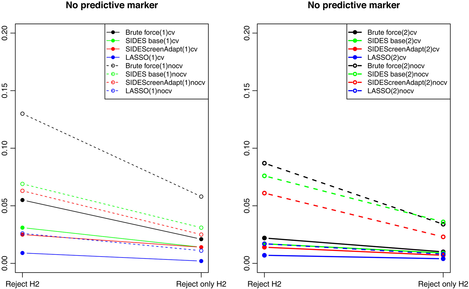
Rejection rates in the identified subgroup at FA for the scenario with no predictive marker and depth = 1 (left panel) and depth = 2 (right panel). Solid lines indicate search strategies followed by cross-validated estimates of treatment effect in identified subgroups. Dashed lines—when no cross-validation was used. Reject H2 is when the null hypothesis was rejected in the identified subgroup and Reject only H2 is when the null hypothesis was rejected in the identified subgroup and not in the overall population

To gain a better insight into the accuracy of cross-validation estimates of the identified subgroup effects, we summarized simulation estimates of the adjusted, unadjusted, and true hazard ratios within the subgroups for all four-search methods under the six scenarios using boxplots. As an illustration, we present only results for the SIDES Base (Figure 7) and SIDEScreen Adaptive (Figure 8). First, observe that the cross-validated hazard ratios are centered around the true hazard ratios while the unadjusted ratios are biased downward, which indicates the “over-optimism bias.” Comparing the unadjusted estimates for the SIDES Base and SIDEScreen Adaptive, we notice that, while the SIDES Base has largely overoptimistic unadjusted hazard ratios (especially for depth = 2), the over-optimism in the SIDEScreen Adaptive is smaller. An appealing aspect of the SIDEScreen Adaptive compared to more greedy search methods, including the SIDES Base, is that it already incorporates protection against false discovery as part of its search method, hence a lesser need to apply shrinkage to the naive estimates of the treatment effect in the subgroups. This is also seen when examining Figure 5, noting the adjusted and unadjusted results (represented by the dashed and solid lines) are closer for the SIDEScreen Adaptive compared to the SIDES Base.

FIGURE 7.

Boxplots comparing cross-validated (CV. HR) versus unadjusted (Unadj. HR) versus true hazard ratios under SIDES base method

FIGURE 8.

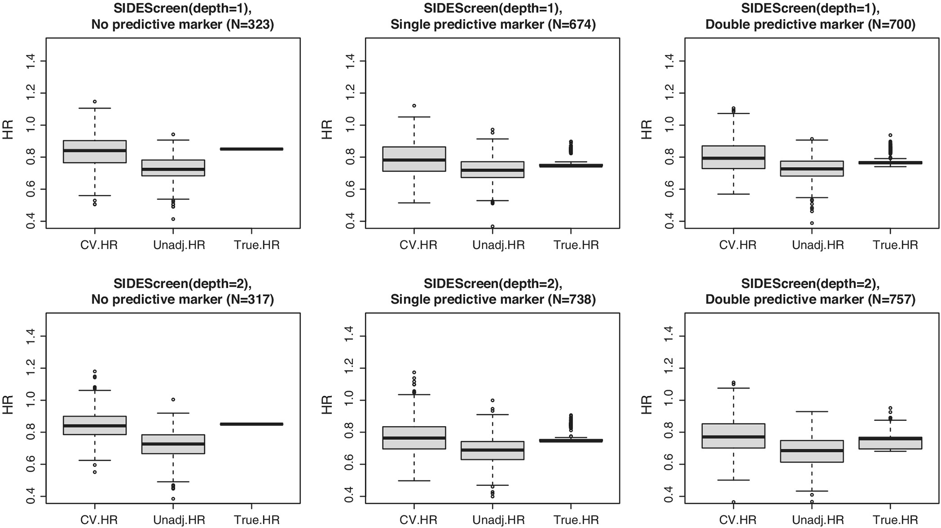
Boxplots comparing cross-validated (CV. HR) versus unadjusted (Unadj. HR) versus true hazard ratios under SIDEScreen Adaptive method

4 |. CONCLUSIONS

This paper evaluates operating characteristics of an adaptive clinical trial with the data-driven selection of a sub-population at an interim time point. We considered hypothetical scenarios when data-driven subgroup discovery methods may be beneficial as evaluated by criteria reflecting the perspectives of various stakeholders, for example, the trial’s sponsor (measured by the statistical power), the society at large (measured by the public utility) and the patient (e.g., reflected in the probability of early stopping for futility). To illustrate benefits of examining sub-population effects, we chose a scenario with a relatively weak overall treatment effect and substantial treatment effect in a subgroup.

If at least one strong predictive biomarker is expected in the set of candidate biomarkers, greater utility can be generally achieved by data-driven sub-population selection as compared with the traditional adaptive design allowing for stopping if a futility criterion has been met. Comparing a biomarker-driven with the standard fixed design may be misleading as the public utility does not reflect patient’s losses resulting from receiving an ineffective treatment. We found that the benefits of more complex subgroup identification strategies involving more than a single biomarkers might not provide advantages even for scenarios where the largest treatment effect is in subgroups defined by two biomarkers. These findings seem reasonable given that the consequence of choosing a subgroup defined by multiple biomarkers will result in decrease in statistical power for detecting treatment differences.

The SIDEScreen Adaptive method was the most competitive method for subgroup discovery that provided a desirable balance between the true positive and false positive rates. The Brute Force method performed well with respect to the true positive rate but this came at a price of an inflated false positive rate. If there is a good belief that one predictive biomarker exists out a few candidate biomarkers, Brute Force may be a sufficient method for subgroup discovery. One disadvantage of using either SIDES method is the need for cross-validation, which means that the LASSO could be more appealing since the cross-validation (for complexity control) is incorporated into the LASSO algorithm. We found that non-cross validated procedures resulted in higher power/utility. However, this may results in a higher risk of selecting a spurious subgroup for the final analysis.

As stated previously, most of the current research on subgroup discovery does not incorporate methods to test for the treatment effect in the overall population. Our research framework supports a comparison of popular methods for implementing subgroup discovery as well as procedures for evaluating treatment effects in both populations while controlling the Type I error rate. These methods are most useful when searching for a single biomarker and should be considered when designing adaptive trials with population selection. Ultimately, our results demonstrate that data-driven subgroup identification techniques are possible within the adaptive clinical trial design and could retain the resources used by a sponsors from development of a novel treatment.

In the presented simulations, we considered a situation common in clinical practice when the sponsor’s decisions are based on conditional power at interim analysis. Then we assess these decisions via simulations using various criteria including the utility function (7). Alternatively, we could consider a more complex scenario when the sponsor is making decisions at interim by maximizing expected utility evaluated via predictive distributions of future outcomes (estimated from the data available at interim), consistently with the assessment criterion used in the simulations. This is the topic of our future research.

Another extension to be considered is to include more challenging data simulation models, for example, consider models with prognostic effects that may obscure identifying predictive effects. Lastly, in this paper we looked at a seamless two-stage design, and it may be of interest to compare it with a “benchmark strategy” where the learnings from the first stage are subsequently applied to the stage 2 trial, and the final analysis is based solely on the data from stage 2.

DATA AVAILABILITY STATEMENT

Data sharing not applicable to this article as no real datasets were used.

REFERENCES

- 1.Lipkovich I, Dmitrienko A, D’Agostino B Sr. Tutorial in biostatistics: data-driven subgroup identification and analysis in clinical trials. Stat Med. 2017;36:136–196. doi: 10.1002/sim.7064 [DOI] [PubMed] [Google Scholar]
- 2.Jiang W, Freidlin B, Simon R. Biomarker-adaptive threshold design: a procedure for evaluating treatment with possible biomarker-defined subset effect. J Natl Cancer Inst. 2007;99(13):1036–1043. [DOI] [PubMed] [Google Scholar]
- 3.Renfro L, Coughlin C, Grothey A, Sargent D. Adaptive randomized phase II design for biomarker threshold selection and independent evaluation. Chin Clin Oncol. 2014;3:1–14. [DOI] [PMC free article] [PubMed] [Google Scholar]
- 4.Spencer A, Harbron C, Mander A, Wason J, Peers I. An adaptive design for updating the threshold value of a continuous biomarker. Stat Med. 2016;35:4909–4923. [DOI] [PMC free article] [PubMed] [Google Scholar]
- 5.Du Y, Rosner G, Rosenblum MD. Phase II Adaptive Enrichment Design to Determine the Population to Enroll in Phase III Trials, by Selecting Thresholds for Baseline Disease Severity. Johns Hopkins University, Department of Biostatistics Working Papers; 2018:290. [Google Scholar]
- 6.Diao G, Dong J, Zeng D, Ke C, Rong A, Ibrahim JG. Biomarker threshold adaptive designs for survival endpoints. J Biopharm Stat. 2018; 28(6):1038–1054. [DOI] [PMC free article] [PubMed] [Google Scholar]
- 7.Lai T, Lavori P, Liao O. Adaptive choice of patient subgroup for comparing two treatments. Contemp Clin Trials. 2014;39:191–200. [DOI] [PMC free article] [PubMed] [Google Scholar]
- 8.Freidlin B, Simon R. Adaptive signature design: an adaptive clinical trial design for generating and prospectively testing a gene expression signature for sensitive patients. Clin Cancer Res. 2005;11:7872–7878. [DOI] [PubMed] [Google Scholar]
- 9.Freidlin B, Jiang W, Simon R. The cross-validated adaptive signature design. Clin Cancer Res. 2010;16:691–698. [DOI] [PubMed] [Google Scholar]
- 10.Zhang Z, Li M, Lin M, Soon G, Greene T, Shen C. Subgroup selection in adaptive signature designs of confirmatory clinical trials. J R Stat Soc Ser C Appl Stat. 2017;66:345–361. [Google Scholar]
- 11.Zhang Z, Chen R, Soon G, Zhang H. Treatment evaluation for a data-driven subgroup in adaptive enrichment designs of clinical trials. Stat Med. 2018;37:1–11. doi: 10.1002/sim.7497 [DOI] [PubMed] [Google Scholar]
- 12.Simon N, Simon R. Adaptive enrichment designs in clinical trials. Biostatistics (Oxford, England). 2013;14:513–625. [DOI] [PMC free article] [PubMed] [Google Scholar]
- 13.Simon N, Simon R. Using Bayesian modeling in frequentist adaptive enrichment designs. Biostatistics (Oxford, England). 2018;19: 27–41. [DOI] [PMC free article] [PubMed] [Google Scholar]
- 14.Li J, Zhao L, Tian L, et al. A predictive enrichment procedure to identify potential responders to a new therapy for randomized, comparative controlled clinical studies. Biometrics. 2015;72:877–887. [DOI] [PMC free article] [PubMed] [Google Scholar]
- 15.Xu Y, Constantine F, Yuan Y, Pritchett Y. ASIED: a Bayesian adaptive subgroup-identification enrichment design. J Pharm Stat. 2020; 30:623–638. [DOI] [PubMed] [Google Scholar]
- 16.Proschan MA, Lan KG, Whites JT. Statistical Monitoring of Clinical Trials. 1st ed. Springer; 2006. [Google Scholar]
- 17.Wang SJ, James Hung HM, Tsong Y, Cui L. Group sequential test strategies for superiority and non-inferiority hypotheses in active controlled clinical trials. Stat Med. 2001;20(13):1903–1912. doi: 10.1002/sim.820 [DOI] [PubMed] [Google Scholar]
- 18.Brannath W, Posch M, Bauer P. Recursive combination tests. J Am Stat Assoc. 2002;97(457):236–244. [Google Scholar]
- 19.Hommel G Adaptive modifications of hypotheses after an interim analysis. Biom J. 2001;43(5):581–589. [Google Scholar]
- 20.Alemayehu D, Chen Y, Markatou M. A comparative study of subgroup identification methods for differential treatment effect: performance metrics and recommendations. Stat Methods Med Res. 2018;27(12):3658–3678. [DOI] [PubMed] [Google Scholar]
- 21.Huber C, Benda N, Friede T. A comparison of subgroup identification methods in clinical drug development: simulation study and regulatory considerations. Pharm Stat. 2019;18(5):600–626. [DOI] [PMC free article] [PubMed] [Google Scholar]
- 22.Loh WY, Cao L, Zhou P. Subgroup identification for precision medicine: a comparative review of 13 methods. WIREs Data Min Knowl Discov. 2019;9(5):e1326. [Google Scholar]
- 23.Lipkovich I, Dmitrienko A, Denne J, Enas G. Subgroup identification based on differential effect search—a recursive partitioning method for establishing response to treatment in patient subpopulations. Stat Med. 2011;30(21):2601–2621. doi: 10.1002/sim.4289 [DOI] [PubMed] [Google Scholar]
- 24.Lipkovich I, Dmitrienko A. Strategies for identifying predictive biomarkers and subgroups with enhanced treatment effect in clinical trials using SIDES. J Biopharm Stat. 2014;24(1):130–153. [DOI] [PubMed] [Google Scholar]
- 25.Tibshirani R Regression shrinkage and selection via the Lasso. J R Stat Soc B Methodol. 1996;58(1):267–288. [Google Scholar]
- 26.Graf A, Posch M, König F. Adaptive designs for subpopulation analysis optimizing utility functions. Biom J. 2015;57:76–89. [DOI] [PMC free article] [PubMed] [Google Scholar]
- 27.Youden WJ. Index for rating diagnostic tests. Cancer. 1950;3(1):32–35. [DOI] [PubMed] [Google Scholar]
- 28.Sasaki Y The Truth of the F-Measure. 1st ed. School of Computer Science, University of Manchester; 2007. [Google Scholar]
Associated Data
This section collects any data citations, data availability statements, or supplementary materials included in this article.