Using machine learning surrogate modeling for faster QSP VP cohort generation

Abstract

Virtual patients (VPs) are widely used within quantitative systems pharmacology (QSP) modeling to explore the impact of variability and uncertainty on clinical responses. In one method of generating VPs, parameters are sampled randomly from a distribution, and possible VPs are accepted or rejected based on constraints on model output behavior. This approach works but can be inefficient (i.e., the vast majority of model runs typically do not result in valid VPs). Machine learning surrogate models offer an opportunity to improve the efficiency of VP creation significantly. In this approach, surrogate models are trained using the full QSP model and subsequently used to rapidly pre‐screen for parameter combinations that result in feasible VPs. The overwhelming majority of parameter combinations pre‐vetted using the surrogate models result in valid VPs when tested in the original QSP model. This tutorial presents this novel workflow and demonstrates how a surrogate model software application can be used to select and optimize the surrogate models in a case study. We then discuss the relative efficiency of the methods and scalability of the proposed method.

INTRODUCTION

Mechanistic quantitative systems pharmacology (QSP) models represent processes relevant to clinical disease progression and the pharmacological effects of therapeutic interventions. They typically draw on a wide range of in vitro, nonclinical, and clinical knowledge and data to identify and quantify the biological processes that give rise to clinical symptoms and the mechanisms by which existing or novel therapies interact with the disease biology. QSP models are thus data‐, knowledge‐, and hypothesis‐based. ¹ Significant biological uncertainty and variability typically remains so no single instance of a QSP model—its equations and parameter values—can be said to be the definitive biology model. QSP modeling commonly uses multiple “virtual patients” (VPs)—distinct sets of parameter values that capture a range of biological hypotheses and variability—to capture the range of biological behaviors observed in existing clinical data and to facilitate exploration of the likely range of biological responses to novel interventions. ²

To de‐risk the development of novel therapies, it is desirable to create a wide range of VPs to fully explore the feasible space defined by constraints on the model behavior. A conceptually straightforward method of generating VPs is illustrated in ref. 3. Parameters are sampled, the model is run through relevant simulated protocols, and the simulated model results are compared to clinical constraints. Parameter sets that produce simulation results that satisfy all constraints are deemed “plausible” VPs. This process works but can be very low‐yield and simulating the full QSP model can be computationally expensive. Biological parameters are highly interdependent in ways that are not known a priori, so random sampling tends to result in combinations that do not produce valid model behaviors that pass all constraints. Several methodologies have been developed in recent years to facilitate creating VPs or virtual populations. ⁴ , ⁵ , ⁶ In this tutorial, we describe an alternative novel workflow taking advantage of surrogate modeling to pre‐screen parameter sets so that only the most promising combinations of parameters are simulated in the full QSP model.

Such use of machine learning techniques for VP or “virtual twin” generation has recently been illustrated in cardiac models, where generation of “families of models” (i.e., multiple copies of a single mathematical model but with different parameter values) has been of interest for some time. ⁷ , ⁸ In one example, ⁹ surrogate models based on Support Vector Machines were used in place of full model simulations to efficiently generate a family of models consistent with clinical data. In another example, ¹⁰ a generative adversarial network approach was used to generate a family of models and infer parameter distributions for a model of myofilament contraction. In this tutorial, we elaborate on the use of surrogate models for VP development in the context of QSP modeling. We introduce a practical general workflow that does not depend on specific model properties or available data. We discuss considerations for the choice of surrogate models and their validation. Finally, we describe the surrogate model generation process step by step in the Regression Learner App ¹¹ and include scripts in the supplemental materials to facilitate hands‐on learning.

Surrogate modeling is a special case of supervised machine learning applied in engineering design, ¹² where a model faster to simulate than the full QSP model is trained to replicate the results of the full QSP model for predefined conditions. The workflow is illustrated in Figure 1, Stage 2. The development of a surrogate model consists of three major steps: (1) relevant parameters are sampled, and the full QSP model is simulated to generate the corresponding model response, (2) a surrogate model is trained to capture the relationships between input parameters and the QSP model response, (3) eventually, the surrogate model can be used for prediction because it can be evaluated on new parameter values to generate the response that the full QSP model is likely to produce.

FIGURE 1.

General workflow for the creation of surrogate models from data. The first stage generates training data from the QSP model. The second uses generated data to train a surrogate and test its performance. Finally, the predictions made by the trained surrogate model are used to filter parameter sets and generate viable VPs. QSP, quantitative systems pharmacology; VP, virtual patient.

The workflow shown in Figure 1 summarizes the workflow of applying surrogate modeling to QSP VP creation. In Stage 1, the full QSP model is simulated to create a training set used to train a surrogate model for each model response in Stage 2. Stage 3 consists of a pre‐screen phase, where the VP generation of sampling parameters, predicting responses, and rejecting or accepting the parameter set as a plausible VP is performed using the surrogate models, which run almost instantaneously. The second phase of Stage 3 validates the pre‐screened VPs against the full QSP model.

In this tutorial, we discuss this novel workflow, including the process of generating and applying the surrogate models, by example of a previously established QSP model of psoriasis. The psoriasis QSP model is a mechanistic model that represents key biological processes involved in psoriasis pathophysiology and response to therapy. Cellular dynamics of keratinocytes, corneocytes, dendritic cells, macrophages, Th1, cytotoxic T cells, Th17 cells, and regulatory T cells are explored, as are the production and effects of cytokines involved in psoriasis. The psoriasis model was implemented in SimBiology (MATLAB, 2020). ¹³ An exported version of this model, which was used for the generation of training data and VP cohort simulation, is included in the Supplementary Materials.

NOVEL VP CREATION WORKFLOW

Stage 1: Generate training data set

Step 1.1: Choose parameters

QSP models often have dozens or even hundreds of parameters, and only a subset of these parameters is generally chosen for VP creation in practice. Choosing which parameters to vary between VPs is usually informed by sensitivity analysis and information about reported or hypothesized biological variability. ¹ This preliminary step of choosing parameters can be quite complex and is not a focus of this tutorial. However, we provide general guidelines and tools for parameter selection in the discussion about Stage 2, Step 2.1, below. For illustrative purposes in this tutorial, and to keep the examples in the scripts tractable, the number of parameters to be varied between VPs was limited to five (Table 1). These parameters were chosen because outcomes of interest in the psoriasis model were sensitive to these parameters. Furthermore, variability in these parameters across VPs was expected to lead to variability in cell populations that play a role in disease pathophysiology and response to treatments in psoriasis. The parameters' ranges of variability are described in relation to an existing reference VP in the psoriasis model. All other parameters in the model retain the same value as in the reference VP.

TABLE 1.

Parameters sampled for VP generation.

Parameter	Fold change
KC_Basal_Skin_density_prolif_Imax	0.5–1
KC_Basal_Skin_stim_prolif_k	0.5–2
Mac_Act_Skin_clear_k	0.5–2
Proinflam_Cyt_Skin_clear_k	0.5–2
Th17_Act_Skin_clear_k	0.5–2

Abbreviation: VP, virtual patient.

Note: Range is expressed as ‐fold change from a reference VP.

Typical VP generation efforts may involve 20–30 parameters, depending on the specifics of the model and the research question under investigation, but care should be taken to limit the VP generation workflow to using only sensitive parameters in order to avoid incurring substantial computational overhead to create VPs that are not meaningfully different.

Step 1.2: Sample parameters

Chosen parameters are sampled using distributions that are typically not known a priori but informed by data or prior experience working with the model. Variability was defined in terms of fold change from the reference VP parameter value, and a uniform sampling distribution was chosen for the psoriasis case study. Each set of sampled values for the five chosen parameters is referred to as a parameter set in this tutorial.

Step 1.3: Simulate QSP model

We use the sampled parameters and simulate the QSP model in this step. This step should include running any protocols where data that can be applied as constraints for plausible VPs in Step 1.3 of the workflow are available. For example, if clinical data for existing therapy responses exists, it could be applied in Step 1.3 to rule out certain implausible VPs if their responses to the treatment fall outside the observed responses. In the current example, we simulate only an untreated protocol (i.e., disease processes with no therapy or other perturbation applied) for illustrative purposes.

Steps 1.1–1.3 are performed to generate the training data set. The optimal size of the data set required to train the surrogates has not been fully determined to date. However, an initial investigation specific to this case study is provided in the Supplementary Material. The size and complexity of the model, as well as the number of parameters and output constraints, should be factors to consider. Training data for the surrogate models were generated using sample simulation data from the full QSP model for this case study. A set of 10,000 parameter sets was created within target fold change ranges, as shown in Table 1, through uniform random sampling. Each parameter set was simulated in the full QSP model to generate response data. Responses for 11 constrained model species were then measured at the final timepoint for each simulation. Training data tables were created for each constrained model species, with each model species end point value serving as the output variable for the data set and the five sampled parameter values serving as the predictor variables for the data set.

Stage 2: Generate surrogate models

This section introduces intuitive guidelines for choosing the best type of surrogate model to fit the data. We also present a methodology for training surrogate models and metrics to assess how accurately the surrogate model approximates the full QSP model.

We use the Regression Learner App ¹¹ to train surrogate models. This app provides step‐by‐step support for parameter selection and data preparation, as well as surrogate model training and validation. We use the Regression Learner App to illustrate the workflow for the creation of surrogates, however, other tools for fitting, validating, and evaluating surrogates are available. We refer to ref. 14 and the references therein for an overview. All guidelines and intuition for the workflows described in this tutorial are equally applicable and are not specific to the Regression Learner App.

Step 2.1: Training setup: Parameter selection, training data test data, validation scheme

Parameter selection

The sampled parameters in the QSP model are often called features or predictors in the context of machine learning. We first identify relevant parameters that explain the QSP model's response variability, as mentioned in Step 1.1. ¹⁴ Sensitivity analyses and prior knowledge can be used to identify important parameters. Plotting the QSP model response against single parameter variation and keeping all other parameter values fixed at their values in the reference VP is a visual way to assess the importance of parameters for training a surrogate model (Figure 2, left). Parameters that cause larger variations in QSP model responses are generally good candidates to include in training surrogate models. Conversely, parameters that do not affect QSP model responses should be excluded from the surrogate model creation to ensure the existence of a unique surrogate model. Care should be taken to curate the data set to identify the chosen parameters uniquely.

FIGURE 2.

Parameter/feature selection by visual inspection of the response versus input parameter plot (left panel) and the application of feature ranking algorithms (right panel).

Besides sensitivity analysis, prior knowledge, and visual inspection, other methods for parameter selection such as the minimum redundancy maximum relevance method ¹⁵ or a neighborhood component analysis ¹⁶ can be used. Filter‐type parameter selection algorithms, such as RReliefF ¹⁷ or F‐tests, that search for a subset of parameters optimally fitting measured model responses, can also be used for parameter selection. All methods mentioned above are also called feature selection or feature ranking methods in the context of machine learning (Figure 2, right). They can each yield different importance rankings of the parameters as every method focuses on different aspects of how parameters affect QSP model responses. Therefore, we recommend considering several parameter selection methods, ensuring that no critical parameter is left out when training the surrogate model.

We also briefly mention feature engineering besides parameter (feature) selection. Feature engineering is a technique transforming and combining sets of parameters in a way beneficial for training surrogate models. Automatic feature engineering can be used to increase the predictive power of surrogate models ¹⁸ to find optimal transformations along with the best combinations of parameters.

Training data, test data and validation scheme

We split the data into a training set and a test set, creating a surrogate response of a QSP model response. Reasonable ratios are 70%–80% training data and 20%–30% test data. Figure 3 shows how to specify the data set and the split into training and test data in the Regression Learner App. The surrogate model is created based on training data only. The test data is only used after the training of the surrogate model to assess its accuracy (i.e., how well it approximates the full QSP model response). A validation metric (e.g., the root mean squared error [RMSE] or mean absolute error), is computed for this assessment. Re‐substitution validation (i.e., computing validation metrics on the training data) should be avoided. It generally yields unrealistically high validation accuracy, even though the predictive accuracy for parameter sets not used during training might be low. ¹⁹

FIGURE 3.

Selection of a validation scheme in the Regression Learner App, such as cross‐validation to minimize overfitting and data splitting to evaluate final model performance on unseen data.

Step 2.2: Surrogate model selection and training

Building intuition: Choosing the right surrogate type

Using surrogate models is an inexpensive way to evaluate full QSP model approximations. The general form of a surrogate model is $r=f\left(p,\theta \right),$ where $f$ is the surrogate that maps parameters $p$ to the approximated response $r$. Surrogate models often also depend on so‐called hyperparameters $\theta$ that allow modelers to improve the accuracy of the full QSP model approximation.

To determine the right type of surrogate to approximate QSP models, we characterize the model responses by their degree of nonlinearity, ranging from constant or linear, slightly nonlinear (e.g., solutions to slow mass action kinetics), highly nonlinear (e.g., oscillatory kinetics), to abrupt changes (e.g., fast reaction kinetics and phase transitions). Different types of surrogate models exist for each of these characteristics. Linear or quadratic model responses are best approximated using linear or polynomial regression surrogate models. Nonlinear model responses, including oscillatory responses, can typically be well approximated using spline interpolation, Bezier curves, Fourier analysis, or nonparametric models like radial basis functions (RBFs) or Gaussian process regression models. ²⁰ RBFs and Gaussian processes are useful for approximating data on scattered (e.g., randomly sampled) parameter sets particularly. The amount of data required to train accurate surrogate models increases with the degree of nonlinearity of the full QSP model responses in general.

We visualize sampled QSP model responses around the reference VP (see Table 1) to see which type of surrogate is best for the psoriasis model. Figure 4 shows the sampled QSP model response Th17_total. The response shows a nonlinear but smooth behavior. Following the classification above, nonparametric surrogates, such as RBFs or Gaussian process regression models, are well‐suited for the approximation of the QSP model responses. The response variation is most significant for parameter values approaching the boundaries of the parameter domain, suggesting the training and test data should contain samples from those regions. The randomly sampled data set (see Step 1.2) is also well‐supported by Gaussian process surrogates or RBFs, further suggesting those surrogates are suitable to approximate these kinds of nonlinear QSP model responses.

FIGURE 4.

Simulated Th17_total response at steady state around nominal parameter values listed in Table 1.

Because Gaussian processes are good candidates to approximate the psoriasis model, we discuss those surrogate models in greater detail. Gaussian processes can be expressed as follows:

$$f\left(\overrightarrow{p,}\theta \right)=\sum _{j=1}^N{\alpha }_{j}k\left({\overrightarrow{p}}_j,\overrightarrow{p};\theta \right).$$

The basis‐functions $k\left({\overrightarrow{p}}_j,\overrightarrow{p};\theta \right)$ for $N$ parameter sets ${\left\{{\overrightarrow{p}}_j\right\}}_{j=1}^N$ are determined by a kernel function $k$ describing the correlation between samples ${\overrightarrow{p}}_j$ and parameter values $\overrightarrow{p}$ for which the model response is unknown. The kernel function has free parameters, $\theta$, the hyperparameters, that can be used to improve the approximation between the surrogate model and the QSP response. A simple example for a kernel function is the square‐exponential kernel:

$$k\left(\overrightarrow{p},\overrightarrow{q}\right)=\mathit{COV}\left(f\left(\overrightarrow{p}\right),f\left(\overrightarrow{q}\right)\right)={\sigma }^2\exp \left(\frac{{‖\overrightarrow{p}-\overrightarrow{q}‖}^2}{2l^2}\right)$$

with hyperparameters $\theta =\left\{\sigma ,l\right\},$ the kernel variance ${\sigma }^2$ and length scale $l$. Gaussian process regressions have been described in depth. ²⁰ Intuitively, the greater the kernel variance, the better the surrogate can approximate rapid changes in QSP model responses. The length scale reflects the correlation of the QSP model response at different timepoints. Thus, the larger the length scale and the lower the variability over time, the more predictive power the training data has. Conversely, the smaller the length scale and larger the variability, the more flexible the Gaussian process prediction is. The predictive power of training data is smaller, requiring more training data to accurately approximate the QSP model response in those cases. We want to use as much information as possible from available data points to make predictions with a small number of training data and be as flexible as possible to best adapt to nonlinear QSP model behavior in practice. The hyperparameters are optimized to find the best values for a flexible and predictive surrogate model to achieve this goal.

We show Gaussian process surrogates for the Th17_total response in the psoriasis model for varying values of parameter Mac_Act_Skin_clear_k for different length scales $l$ ranging from ${10}^{-5}$ to $0.1$ in Figure 5 to illustrate the importance of hyperparameter optimization. We see that for small length scales, the predictive power of the surrogate on the test set, measured using RMSE, is significantly reduced, whereas choosing a larger length scale yields a good surrogate approximation. Note that the RMSE increases, even on the training data, if the length scale becomes too large. The reason for this is that the Gaussian process becomes too inflexible to even represent the training data accurately. Figure 5 also shows that if the length scale is small, the validation metric on the training data becomes meaningless. The error between the QSP model response and the surrogate model prediction can only be quantified on the independent test data, which was not used for training the surrogate model.

FIGURE 5.

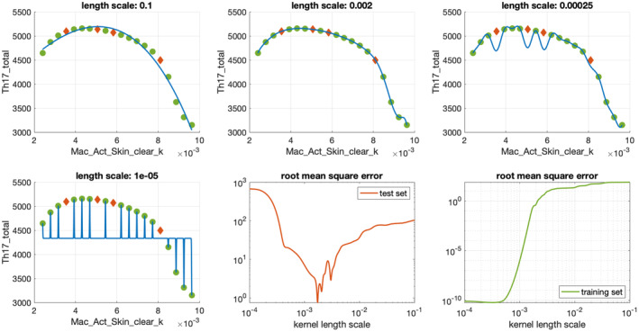
Gaussian process approximation of Th17_total data for a single parameter Mac_Act_Skin_clear_k. Green dots are training data, red diamonds represent test data.

Creating surrogate models in the Regression Learner App

Using the Regression Learner App can automate selecting and training different surrogate models. The app uses k‐fold cross‐validation to determine the best surrogate type to fit the training data. Figure 3 shows a screenshot of the app demonstrating how the k‐fold cross‐validation can be configured. The k‐fold cross validation method splits the training set into k groups, which are also called folds. Typical values for k are 5 or 10, depending on the data set size. During k‐fold cross validation, k surrogate models, one for each fold, are trained. For each surrogate model, one‐fold is held out, and its accuracy is estimated using the validation metric, typically the RMSE, on the held‐out fold. The overall accuracy is then computed by averaging the validation metric of all k surrogate models. The k‐fold cross validation stratifies overfitting bias to k different training sets.

One benefit of k‐fold cross‐validation is that we know the validation metric for the surrogate model without using test data. The surrogate model with the highest average validation metric over all k folds is deemed the best. The best surrogate model is then re‐fitted on the full training set to use all available training data. The final accuracy of the selected surrogate model is then assessed on the test set.

In summary, the k‐fold cross‐validation approach requires k surrogate models to be trained for each type. Therefore, it is beneficial to eliminate surrogate types a priori that are known to be not suitable for approximating the full QSP model response accurately. We already know that Gaussian processes are good candidates for the psoriasis model. Therefore, we restrict the surrogate type to nonlinear models and omit the consideration of linear regression models in the following example.

In Figure 6, various surrogate types, ranging from decision trees, ²¹ support vector machines, ²² neural networks ²³ to Gaussian process models ²⁰ are listed in the Models panel (left) of the Regression Learner App. Running the app yields validation scores for the validation metric specified in Step 2.1 (see Figure 3). We see that the intuitive choice of a Gaussian process regression model from the last section is, in fact, the best surrogate type when we look at the validation score (RMSE) for all models.

FIGURE 6.

Selection of a Gaussian Process Regression model as the best surrogate model for the response Th17_total after parallel training of multiple model types and their hyperparameter optimization. The best model was selected based on its validation root mean squared error and its performance subsequentially quantified on a test set. The left panel shows the list of candidate model types with their validation accuracy. The right panel shows the training summary, the minimum mean squared error for each iteration of the hyperparameter optimization, a residual versus true response plot as well as a predicted response versus true response plot.

The ranking of surrogate models is determined prior to optimizing hyperparameters. The final surrogate model is created using the full training set as well as optimized hyperparameters. The optimization of hyperparameter is performed on the k‐fold split of the training data to improve its accuracy without overfitting to the training data. Note that not all surrogate models in the Regression Learner App support hyperparameter optimization. Therefore, it is recommended to select optimizable versions of all surrogate types and compare their validation score after their hyperparameters have been optimized. In the next Step 2.3, we discuss the validation of fitted surrogate models using the held‐out test data.

The concept of automatic machine learning ²⁴ , ²⁵ can be used to automate surrogate selection, training, and validation. We refer to the provided references for details, however, we want to emphasize that although the automation can be convenient, having intuition about the surrogate selection and fitting process can help to reduce computational overhead (e.g., by a priori limiting the set of surrogate types). The intuition also gives confidence that a good surrogate type is chosen. Within the next Step 2.3 we formalize how to assess the predictive accuracy of surrogates.

Step 2.3: Test/explain surrogate model

Testing the surrogate model

The final validation of the surrogate model's accuracy is performed on the test data, which was not used while training the surrogate model. The validation metrics for the surrogate model are shown in the Summary panel in the Regression Learner App (Figure 6). The validation metric measures the error between the surrogate model and the full QSP model on the test data. Therefore, the lower the value the better. In general, there is a trade‐off between accuracy of the surrogate models and the efficiency of creating them. The surrogate accuracy should be good relative to the context the surrogate is used in. In our use case, for example, we are vetting the surrogate predictions against the QSP model. This provides a safeguard against loss of accuracy of the final virtual population. See Stage 3 and the final discussion of the method below for more details.

The Regression Learner App produces diagnostic plots to further assess the accuracy of the surrogate in addition to the validation metric. The plots include a Predicted versus Actual plot (Figure 6, lower right) and a Residuals plot (Figure 6, lower left), which can be used to detect parameter regions and associated QSP model responses not approximated by the surrogate model accurately.

Moreover, model type and application agnostic techniques are also available to analyze the surrogate model. For example, Shapley values ²⁶ or LIME ²⁷ provide information about the contribution of specific parameters to a model response. This type of analysis shares similarities with a local sensitivity analysis. This additional analysis of the surrogate model can reveal properties, parameter correlations, insensitivities, or aliasing effects within the original QSP model, although not this tutorial's focus.

Further assurance for the accuracy and predictive power of the surrogate model can be obtained within the context in which the surrogate model is used in addition to the assessment of the surrogate model's accuracy using the validation metrics discussed above. In Stage 3, we discuss further validation of the surrogate model predictions for the purpose of generating virtual populations for the study of the psoriasis model.

Stage 3: Generate VPs using surrogate models

The surrogate models can be used to prescreen parameter sets for more efficient VP creation once created. The following sections describe each step. MATLAB ¹³ scripts to create training data, generate surrogate models, and simulate the VP cohort for the psoriasis QSP model are included in the Supplementary Material.

Step 3.1: Sample parameters

The same parameters as in Step 1.1 are sampled. The identical sampling distributions and methods used to generate training data in Steps 1.1 and 1.2 were used in Step 3.1 to generate parameter sets for the updated VP cohort creation workflow for the psoriasis case study.

Step 3.2: Run surrogate models to predict responses

The sampled parameter sets are used as input vectors for the surrogate models. Eleven surrogate models were trained for the psoriasis case study, one for each QSP model response for which there are constraints. Each surrogate model predicts the full QSP model's response for the given parameter set. Prediction of responses by the surrogate models incurs negligible computational costs.

Step 3.3: Prescreen parameter sets based on constraints

Predicted response values generated by the surrogate models for each parameter set are compared to the corresponding data constraints. Each of the 11 responses has associated constraints (Table 2). These values are based on analysis of the literature and primary data suggesting that the values should not fall outside of the observed ranges for VPs of the desired phenotype (i.e., any parameter set that results in responses outside of the constraints should be rejected as not being a plausible VP). The parameter set passes the prescreening step as being a likely plausible VP if all predicted responses for a parameter set satisfy the data constraints.

TABLE 2.

Model species and associated constraints that plausible VPs must meet.

Response	Constraint bounds	Units
SPASI	20–40	–
Basal KC	<44,000	cells/mm2
Differentiated KC	<99,000	cells/mm2
Corneocytes	<77,000	cells/mm2
Dendritic cells	<174,800	cells/mm2
Th17	<10,640	cells/mm2
Treg	<21.280	cells/mm2
IL‐17	<14	cells/mm2
IL‐23	<226	cells/mm2
TNF	<90	cells/mm2

Abbreviations: KC, keratinocyte; VPs, virtual patients.

Step 3.4: Simulate full QSP model for accepted parameter sets

Steps 3.1 to 3.3 are repeated until the desired number of accepted parameter sets have been generated. Based on the surrogate model predictions, the full QSP model is then simulated only for the parameter sets that passed the initial prescreening step in Step 3.3.

Step 3.5: Do final filtering

All parameter sets that passed the surrogate model prescreening are simulated in the full QSP model and QSP model responses are compared again to the corresponding data constraints. Parameter sets that result in responses passing all constraints after simulation in the full QSP model are considered “plausible VPs.” Any parameter sets not satisfying all constraints are removed from the final cohort.

DISCUSSION

Method efficiency

The goal of the novel workflow is to improve VP creation efficiency in QSP modeling. The rate‐limiting step in VP creation is simulating the full QSP model to test whether a sampled parameter set leads to model responses within the data constraints. Surrogate modeling sharply reduced the number of full QSP model simulations that did not lead to plausible VPs in our case example. For example, simulating the QSP model 10,000 times without surrogate models only yielded 638 plausible VPs, whereas 10,000 QSP model runs with surrogate modeling and prefiltered parameter sets resulted in 9604 plausible VPs.

Of course, the surrogate modeling method requires an initial investment in generating the training and test sets and surrogate model training and optimization. This investment must be considered when deciding whether to use the surrogate modeling method. Figure 7 illustrates the VP generation efficiency of both methods as a function of total QSP model simulations. Using the traditional method of generating VPs, a total of 1276 VPs are generated in 20,000 QSP model simulations, whereas the surrogate modeling approach generates 10,242 VPs in 20,000 QSP model simulations (638 VPs generated in the training set and 9604 VPs generated after the creation of the surrogate models). Using the traditional approach, generation of 10,000 VPs took 50 min and 12 s and required 152,498 total simulations in the QSP model, whereas generation of 10,000 VPs using the surrogate modeling approach took 4 min and 25 s (including 50 s to train the models), or less than 1/11 of the total time. All simulations were performed using a laptop with eight cores, 32 GB RAM, and an Intel i7 processor with no parallelization. Additional simulations using a larger training data set (10,000 sampled parameter sets) and using optimized surrogate models were also performed, but were not shown to significantly improve the efficiency of the approach. Please see the supplement for additional discussion of how training set size and hyperparameter optimization influenced VP generation efficiency. The workflow is demonstrated here with a simple example and more complete benchmarking remains to be established, but an ~11‐fold speed‐up in VP creation time in scenarios with more complex models and/or simulation protocols would certainly be a significant improvement and could enable larger VP cohorts or more iterations to refine parameter sampling, filtering criteria, or the underlying model itself.

FIGURE 7.

Efficiency comparison of surrogate modeling method. For the same number of total simulations in the full QSP model, the surrogate modeling workflow generated over 10,000 plausible VPs, while the original QSP model workflow only generated ~1300 plausible VPs. QSP, quantitative systems pharmacology; VP, virtual patient.

Method validation

Unlike in other settings, using surrogate models in QSP VP generation has an obvious built‐in validation step where the sampled parameter sets that passed the prefiltering step are simulated using the full QSP model. Therefore, the risk of moving forward with invalid VPs is minimized.

Nonetheless, whether using the surrogate models introduced any bias into parameter selection or response distributions is worth considering. We compared the VPs generated by the traditional versus the surrogate modeling methods and compared the parameters' and response variables' probability density functions and the pairwise correlations between parameter values (Figure 8).

FIGURE 8.

Comparison of attributes for virtual patientss generated by the traditional workflow (light blue) versus surrogate modeling workflow (dark blue). (a) Probability density functions for sampled parameters after filtering, (b) Probability density functions for observable endpoints after filtering, (c) parameter correlation coefficients for parameters sampled without using surrogate models, and (d) parameter correlation coefficients for parameters sampled using surrogate models.

After filtering, the probability distributions of both sampled parameters and observable end points were nearly identical for both methods (Figure 8a,b). The distributions achieved through both sampling methods were compared quantitatively using the two‐sample Kolmogorov–Smirnov Goodness of Fit test. The observables and parameters were found to come from the same distributions within 5% significance. Correlation coefficients were calculated for each pair of parameters. It was observed that the pairwise relationships between parameters generated using the traditional approach were preserved for the parameter sets sampled by the surrogate models (Figure 8c,d). We conclude that there were no systematic differences between VPs generated by the two methods.

CONCLUSION AND FUTURE DIRECTIONS

We have demonstrated that using surrogate models for QSP VP creation can increase efficiency in modeling scenarios where many VPs are needed. Using existing surrogate modeling software for this purpose was found to be straightforward, and the revised workflow produces VPs with similar attributes as VPs created by other methods. Generating a broad range of VPs with mechanistic and phenotypic variability facilitates staying one step ahead of the data and de‐risking drug development, and the workflow presented here makes this process more efficient. VPs can be developed and simulated to anticipate outcomes ahead of clinical data. When new data become available, they can be used to refine the next generation VP cohort or population, which can then be used to gain additional insights and to predict the next trial outcome. The increased efficiency in VP generation enabled by the workflow using surrogate modeling is thus expected to improve the utility of QSP research across the development pipeline.

The utility of machine learning approaches in conjunction with QSP has already been demonstrated in numerous interesting applications ranging from inferring model structure to elucidating the relationships between biomarkers and endpoints. ²⁸ , ²⁹ , ³⁰ In this tutorial, we have added another exciting possibility of using surrogate models as a stand‐in for full QSP model simulations in VP development. In addition to improving VP creation efficiency, the approach also opens the possibility of better understanding the QSP model itself by facilitating exploration and sophisticated analysis of the parameter and response space. We believe this analysis will soon become an integral tool for QSP modelers.

FUNDING INFORMATION

R.C.M. and C.M.F. are employees of Rosa & Co, LLC. F.A. and J.H. are employees of The MathWorks, Inc/The MathWorks GmbH.

CONFLICT OF INTEREST STATEMENT

The authors declared no competing interests for this work.

Supporting information

SupinfoS1

FigureS1

FigureS2

FigureS3

FigureS4

TableS1

README file

DataS1

DataS2

DataS3

DataS4

DataS5

DataS6

Myers RC, Augustin F, Huard J, Friedrich CM. Using machine learning surrogate modeling for faster QSP VP cohort generation. CPT Pharmacometrics Syst Pharmacol. 2023;12:1047‐1059. doi: 10.1002/psp4.12999

REFERENCES

- 1. Friedrich CM. A model qualification method for mechanistic physiological QSP models to support model‐informed drug development. CPT Pharmacomet Syst Pharmacol. 2016;5:43‐53. [DOI] [PMC free article] [PubMed] [Google Scholar]
- 2. Kansal AR, Trimmer J. Application of predictive biosimulation within pharmaceutical clinical development: examples of significance for translational medicine and clinical trial design. Syst Biol. 2005;152:214‐220. [DOI] [PubMed] [Google Scholar]
- 3. Rieger TR, Allen RJ, Musante CJ. Modeling is data driven: use it for successful virtual patient generation. CPT Pharmacomet Syst Pharmacol. 2021;10:393‐394. [DOI] [PMC free article] [PubMed] [Google Scholar]
- 4. Allen RJ, Rieger TR, Musante CJ. Efficient generation and selection of virtual populations in quantitative systems pharmacology models. CPT Pharmacomet Syst Pharmacol. 2016;5:140‐146. [DOI] [PMC free article] [PubMed] [Google Scholar]
- 5. Rieger TR, Allen RJ, Bystricky L, et al. Improving the generation and selection of virtual populations in quantitative systems pharmacology models. Prog Biophys Mol Biol. 2018;139:15‐22. [DOI] [PubMed] [Google Scholar]
- 6. Cheng Y, Straube R, Alnaif AE, Huang L, Leil TA, Schmidt BJ. Virtual populations for quantitative systems pharmacology models. Methods Mol Biol. 2022;2486:129‐179. [DOI] [PubMed] [Google Scholar]
- 7. Lawson BAJ, Drovandi CC, Cusimano N, Burrage P, Rodriguez B, Burrage K. Unlocking data sets by calibrating populations of models to data density: a study in atrial electrophysiology. Sci Adv. 2018;4:e1701676. [DOI] [PMC free article] [PubMed] [Google Scholar]
- 8. Niederer SA, Aboelkassem Y, Cantwell CD, et al. Creation and application of virtual patient cohorts of heart models. Philos Transact A Math Phys Eng Sci. 2020;378:20190558. [DOI] [PMC free article] [PubMed] [Google Scholar]
- 9. Romero P, Lozano M, Martínez‐Gil F, et al. Clinically‐driven virtual patient cohorts generation: an application to aorta. Front Physiol. 2021;12:713118. [DOI] [PMC free article] [PubMed] [Google Scholar]
- 10. Parikh J, Rumbell T, Butova X, et al. Generative adversarial networks for construction of virtual populations of mechanistic models: simulations to study Omecamtiv Mecarbil action. J Pharmacokinet Pharmacodyn. 2022;49:51‐64. [DOI] [PMC free article] [PubMed] [Google Scholar]
- 11. The MathWorks®, Inc . Regression Learner App (R2022b). Retrieved on October 03, 2022 from https://www.mathworks.com/help/stats/regression‐learner‐app.html
- 12. Guo S. An introduction to surrogate modeling, part I: fundamentals. Data Sci. 2020. Retrieved on May 28, 2023 from https://medium.com/towards‐data‐science/an‐introduction‐to‐surrogate‐modeling‐part‐i‐fundamentals‐84697ce4d241 [Google Scholar]
- 13. The MathWorks®, Inc . MATLAB® Version 9.8 (R2020a). Natick, Massachusetts.
- 14. Guyon I, Elisseeff A. An introduction to variable and feature selection. J Mach Learn Res. 2003;3:1157‐1182. [Google Scholar]
- 15. Ding C, Peng H. Minimum redundancy feature selection from microarray gene expression data. J Bioinform Comput Biol. 2005;3:185‐205. [DOI] [PubMed] [Google Scholar]
- 16. Yang W, Wang K, Zuo W. Neighborhood component feature selection for high‐dimensional data. J Comput. 2012;7:161‐168. [Google Scholar]
- 17. Kononenko I, Šimec E, Robnik‐Šikonja M. Overcoming the myopia of inductive learning algorithms with RELIEFF. Appl Intell. 1997;7:39‐55. [Google Scholar]
- 18. Kuhn M, Johnson K. Feature Engineering and Selection: A Practical Approach for Predictive Models. Taylor & Francis Group; 2019. [Google Scholar]
- 19. Kuhn M, Johnson K. Applied Predictive Modeling. Vol 26. Springer; 2013. [Google Scholar]
- 20. Rasmussen, C. E. & Williams, C. K. Gaussian Processes for Machine Learning. MIT Press; 2006. [Google Scholar]
- 21. Breiman L. Classification and Regression Trees. Routledge; 2017. [Google Scholar]
- 22. Cortes C, Vapnik V. Support‐vector networks. Mach Learn. 1995;20:273‐297. [Google Scholar]
- 23. Nielsen MA. Neural Networks and Deep Learning. Vol 25. Determination Press; 2015. [Google Scholar]
- 24. The MathWorks(R), Inc . The MathWorks®, Inc., AutoML (Automated Machine Learning) Explained. Retrieved on October 3, 2022. https://www.mathworks.com/discovery/automl.html
- 25. Conrad F, Mälzer M, Schwarzenberger M, Wiemer H, Ihlenfeldt S. Benchmarking AutoML for regression tasks on small tabular data in materials design. Sci Rep. 2022;12:19350. [DOI] [PMC free article] [PubMed] [Google Scholar]
- 26. Lundberg SM, Lee S‐I. A unified approach to interpreting model predictions. Adv Neural Inf Process Syst. 2017;30:4765‐4774. [Google Scholar]
- 27. Ribeiro MT, Singh S, Guestrin C. ‘ Why should I trust you?’ Explaining the predictions of any classifier. 2016:1135–1144.
- 28. Zhang T, Androulakis IP, Bonate P, et al. Two heads are better than one: current landscape of integrating QSP and machine learning: an ISoP QSP SIG white paper by the working group on the integration of quantitative systems pharmacology and machine learning. J Pharmacokinet Pharmacodyn. 2022;49:5‐18. [DOI] [PMC free article] [PubMed] [Google Scholar]
- 29. Aghamiri SS, Amin R, Helikar T. Recent applications of quantitative systems pharmacology and machine learning models across diseases. J Pharmacokinet Pharmacodyn. 2022;49:19‐37. [DOI] [PMC free article] [PubMed] [Google Scholar]
- 30. Cheng L, Qiu Y, Schmidt BJ, Wei G‐W. Review of applications and challenges of quantitative systems pharmacology modeling and machine learning for heart failure. J Pharmacokinet Pharmacodyn. 2022;49:39‐50. [DOI] [PMC free article] [PubMed] [Google Scholar]
Associated Data
This section collects any data citations, data availability statements, or supplementary materials included in this article.
Supplementary Materials