Deep Learning-Based TEM Image Analysis for Fully Automated Detection of Gold Nanoparticles Internalized within Tumor Cell

Abstract

Transmission electron microscopy (TEM) imaging can be used for detection/localization of gold nanoparticles (GNPs) within tumor cells. However, quantitative analysis of GNP-containing cellular TEM images typically relies on conventional/thresholding-based methods, which are manual, time-consuming, and prone to human errors. In this study, therefore, deep learning (DL)-based methods were developed for fully-automated detection of GNPs from cellular TEM images. Several models of “you only look once (YOLO)” v5 were implemented, with a few adjustments to enhance the model’s performance by applying the transfer learning approach, adjusting the size of the input image, and choosing the best optimization algorithm. 78 original (12040 augmented) TEM images of GNP-laden tumor cells were used for model implementation and validation. A maximum F1 score (harmonic-mean of the precision and recall) of 0.982 was achieved by the best-trained models, while mean average precision was 0.989 and 0.843 at 0.50 and 0.50–0.95 intersection-over-union threshold, respectively. These results suggested the developed DL-based approach was capable of precisely estimating the number/position of internalized GNPs from cellular TEM images. A novel DL-based TEM image analysis tool from this study will benefit research/development efforts on GNP-based cancer therapeutics, for example, by enabling the modeling of GNP-laden tumor cells using nanometer-resolution TEM images.

1. Introduction

Over the years, various cancer therapeutic approaches utilizing gold nanoparticles (GNPs) have been the subjects of active investigation (Thakor et al., 2011; Jain et al., 2012; Schuemann et al., 2016). For proper understanding of the mechanisms behind such approaches, it is crucial to determine the cellular uptake as well as intracellular locations of GNPs. For example, as summarized elsewhere (Schuemann et al., 2016), numerous computational and in vitro/in vivo studies have been conducted to show drastic radiation dose enhancement in the immediate vicinity (e.g., less than a micrometer) of GNPs and consequent radiosensitization of GNP-laden cells or tumors. In general, the degree of GNP-mediated dose enhancement & radiosensitization is thought to be closely related with the number of GNPs that enter a cell (i.e., internalized GNPs). Techniques such as inductively coupled plasma mass spectrometry, atomic emission spectroscopy (Chithrani et al., 2006), and flow cytometry (Kim et al., 2012) can be employed to determine the amount or number of internalized GNPs (i.e., GNP uptake in cells). While these assay techniques can provide overall amounts of internalized GNPs, they are limited in offering other quantitative information (shape or size, aggregation, and precise intracellular locations of GNPs) that is essential for accurate modeling of GNP-mediated dose enhancement & radiosensitization from a physical point of view.

Transmission electron microscopy (TEM) is one of the powerful tools to investigate nanoparticle uptake and biodistribution, and interaction with cells and tissue components (Malatesta, 2021; Hao et al., 2012; Chen et al., 2011). Given its nanometer resolution, TEM is well suited to address the aforementioned imaging challenge for modeling of GNP-mediated dose enhancement & radiosensitization. In fact, as illustrated in a recent study (Jayarathna et al., 2019), a computational Monte Carlo (MC) model using a TEM image of a GNP-laden cell can be developed successfully. To develop more sophisticated models of GNP-laden cells, it is crucial to analyze as many TEM images of GNP-laden cells as possible (e.g., thousands of TEM images), which can be tedious and time-consuming. Also, manual nanoparticle counting can also be subjective and may lead to incorrect counts due to inter-observer variability (de Boodt et al., 2013). Considering these challenges, it is important to have an easy-to-use technology that can be used for fully automated nanoparticle identification and statistical analysis. This will help researchers take on massive image analysis tasks which otherwise would be considered impractical. In general, the ability to gather the information contained in TEM images on a large scale is beyond the average skills of a human analyst, thus necessitating the development of fully automated systems to process TEM images.

Within the scope of the current investigation, an ideal automated TEM image processing method should be able to perform two tasks. First, it should detect nanoparticles, which includes identification of nanoparticles, and second, allow for localization of the nanoparticles of interest within cellular structures. There is evidence that nanoparticles are distributed heterogeneously throughout the cell and that they aggregate to form clusters (Hainfeld et al., 2004; Schuemann et al., 2016). Clustering of nanoparticles and the non-uniform background of subcellular organelles with differing electron densities due to varying protein and lipid compositions, concentrations, and densities create problems in nanoparticle identification. In this circumstance, it is also difficult to use traditional image processing methods such as thresholding or matrix filtering (Kapur et al., 1985; Ridler & Calvard, 1978). To address these issues, new techniques are required. These are the reasons why deep neural networks or artificial intelligence seem to be especially promising. Computer-aided systems can use artificial intelligence (AI) via deep learning (DL) and machine learning techniques such as convolutional neural networks (CNNs) for autonomous object recognition. CNNs learn to recognize patterns in input images and connect them with predetermined outcomes, such as object recognition or categorization (Azam et al., 2022). For TEM images, only a few investigations on the DL-based particle detector have been performed so far. These include cell counting and detection of nuclei (Xiao & Yang, 2017; Zhu et al., 2017), virus-particle detection (Ito et al., 2018), and metal nanoparticle detection (Oktay & Gurses, 2019; Saaim et al., 2022; Groschner et al., 2021) in TEM images. To the best of our knowledge, there are some studies that assessed GNP uptake using conventional manual approaches (Xie et al., 2017; Carnovale et al., 2019; Tremi et al., 2021). However, there is no prior study that identified various shapes of GNPs, such as cylindrical GNPs, i.e., gold nanorods (GNRs), and spherical GNPs, i.e., gold nanospheres (GNSs), in TEM images of GNP-laden cells using DL. Therefore, effective automated identification and quantification of GNPs in cellular TEM images remains difficult, motivating us to investigate solutions to this difficulty.

Most DL algorithms are used to detect objects using regular segmentation, such as U-net (Ronneberger et al., 2015), mask region-based convolutional networks (Mask RCNN) (He et al., 2017), and fully convolutional networks (FCN) (Long et al., 2014). These strategies require pixel-by-pixel labeling of ground truth objects. This is often difficult if the objects are small. Bounding boxes can be used to create localizations of objects. This allows us to train an object detection model that can recognize and detect multiple objects, making it adaptable. There are two types of DL-based object detection algorithms: single-stage regression-based and two-stage region-based models. A two-stage detection model is built on region suggestions generated during the first stage. These suggestions can then be used to extract features for classification regression, region of interest (ROI) pooling, and bounding box (Ren et al., 2017). Examples of two-stage detection algorithms include region-based convolution neural networks (R-CNN) (Girshick et al., 2013), spatial pyramid pooling network (SPP-Net) (He et al., 2015), fast region-based convolutional neural networks (Fast R-CNN) (Girshick, 2015), and faster region-based convolution neural network (Faster R-CNN) (Ren et al., 2017). Two-stage object detection algorithms such as faster R-CNN have been used for many applications, including fruit detection in orchard (Sa et al., 2016), cervical spinal cord injury detection on magnetic resonance imaging (Ma et al., 2020), coronavirus detection on chest radiographs (Shibly et al., 2020), cancer cell detection on phase-contrast microscopy images (Zhang et al., 2016), as well as automatic car accident detection (Tian et al., 2019). The two-step detection method is slow and unsuitable for real-time applications, despite its high localization accuracy and recognition accuracy. Single-stage detectors, on the other hand, address object detection as a regression task. They take the single complete image as input and output the class probabilities and several bounding boxes simultaneously (Liu et al., 2016). The model runs much faster than two-stage object detectors. Most popular single-stage object detectors include single shot detector (SSD) (Liu et al., 2016), RetinaNet (Lin et al., 2017), you only look once (YOLO) (Redmon et al., 2015), EfficientDet (Tan et al., 2019) etc. YOLO is fast, accurate, and one of the most well-known single-stage object detection algorithms nowadays. It was first introduced in 2015 through a research paper (Redmon et al., 2015). The algorithm was then improved continuously (YOLOv2 (Redmon & Farhadi, 2016), YOLOv3 (Redmon & Farhadi, 2018), YOLOv4 (Bochkovskiy et al., 2020), and YOLOv5 (Jocher et al., 2022)) to achieve the best object detection capability.

This research presents a DL-based method for fully automated detection of internalized GNPs from cellular TEM images. Ultralytics’ YOLOv5 system (Jocher et al., 2022) was used for the current investigation. This system can be used as a foundation for a low-cost, readily deployable GNP detection system that is also more accurate and much quicker than the conventional methods. In real-time, our method can detect intracellularly distributed GNPs in various shapes including GNRs and GNSs. As such, it can be used as an essential tool that allows for the creation of realistic nanometer-resolution TEM-based models of GNP-laden cells. The availability of such models will likely help unravel the exact mechanisms behind GNP-based cancer therapeutic approaches, such as GNP-mediated dose enhancement & radiosensitization which was the main driver for the current investigation.

2. Methods

2.1. Datasets

We examined two separate sets of TEM images obtained from distinct cell types and GNP treatments. The first set (TEM1) included 57 TEM images acquired from human colorectal tumor cells that were treated with GNRs (10 nm in diameter and 40 nm in height). The second set (TEM2) consisted of 21 TEM images derived from pancreatic tumor cells that underwent treatment with GNSs (5 nm in diameter). The current TEM imaging work was performed, following the procedures described elsewhere (Wolfe et al., 2015). Briefly, thin slices of the cell were prepared using a Leica Ultramicrotome (Leica Microsystems Inc., Deerfield, IL) and then stained with uranyl acetate and lead citrate in a Leica EM Stainer. Bright field TEM imaging was performed using a JEM 1010 transmission electron microscope (JEOL, USA, Inc., Peabody, MA) at an accelerating voltage of 80 kV. Digital images were obtained using an AMT imaging system (Advanced Microscopy Techniques Corp., Danvers, MA). The acquired TEM images were employed to develop an image analysis model for identifying and quantifying GNPs in cell structures. These images also showed a variation in magnification. Some images were taken at 50000× magnification, while others were taken at 25000×. All GNR-containing images were nanometer-resolution at 2256×2448 pixels (single pixel size 1.34 nm × 1.34 nm and 2.69 nm × 2.69 nm for 50000× and 25000× magnification, respectively.), and all GNS-containing images had a resolution of 1024×1184 (single pixel size 5.43 nm × 5.43 nm for 25000× magnification). We first selected 33 GNR and 9 GNS images for model training and the rest for independent testing. The remaining test set contained 36 raw TEM images that were not part of the training dataset. No further image processing or alterations were done to them. Note both GNSs and GNRs are referred to hereafter as GNPs. Since TEM images have a higher resolution, resizing them is not reasonable as the nanoparticle details are lost when reduced to a smaller size. This problem was resolved by manually cropping images with higher resolution to images of 1024×1024 for training. The size problem is only present during training because YOLO models can detect objects in larger images once they are trained. Using a YOLO model trained on patches of lower resolution images and by simply varying the input image size, it can be used to detect an object on any higher resolution original images. Table 1 provides a comprehensive summary of the original TEM datasets used in this study.

Table 1.

Summary of original transmission electron microscopy (TEM) datasets, presenting details on cell types, gold nanoparticle (GNP) types, GNP dimensions, the number of images, image dimensions in pixels, magnification levels for each dataset, and the distribution of images used for both model development and independent performance testing.

TEM Set	Tumor Cell Type	GNP Type	GNP Dimension (nm)	Number of Original Images	Image Dimension (pixel)	Magnification	Number of Original Images Used for Model Development	Number of Original Images Used for Independent Testing
TEM1	Colorectal	GNRs	10 (diameter) 40 (height)	57	2256×2448	50000, 25000	33	24
TEM2	Pancreatic	GNSs	5 (diameter)	21	1024×1184	25000	9	12

Thousands of images are often required to train a CNN model. This is difficult to do experimentally or economically. Data augmentation might be an alternative method to achieve our goal in this situation. It takes existing training datasets and creates significantly modified versions. This technique addresses the limited data problem by increasing the size of the training data. It can then be used to develop more robust DL models. Since the background will not affect our object detection work as the object detection only looks at the target information (localization box, class label), our TEM images are unaffected by data augmentation. For this study, two-stage data augmentation techniques were used. In the first stage, we created 344 augmented TEM images from 42 original images. These images were called Dataset1. This was done by random rotation, zooming, and reflection fill. These techniques produced more images with more GNPs per image shown in Figure 1. It is important to note that the YOLOv5 model requires supervision during object detection training, which is achieved through bounding box annotations. This process involves (a) creating a box around each object to identify it and (b) labeling each box with the object’s class. To perform this task, we utilized LabelImg (an open-source data annotation tool) (Tzutalin, 2015). This tool enabled us to create bounding boxes around objects in TEM images and retrieve their coordinates. By using LabelImg, we drew bounding boxes around all GNPs, ensuring that each box encompassed the entire structure we aimed to detect. The GNP annotations were automatically saved in the corresponding YOLO format, with annotations normalized according to the image size and constrained within the range of 0–1.

Fig. 1.

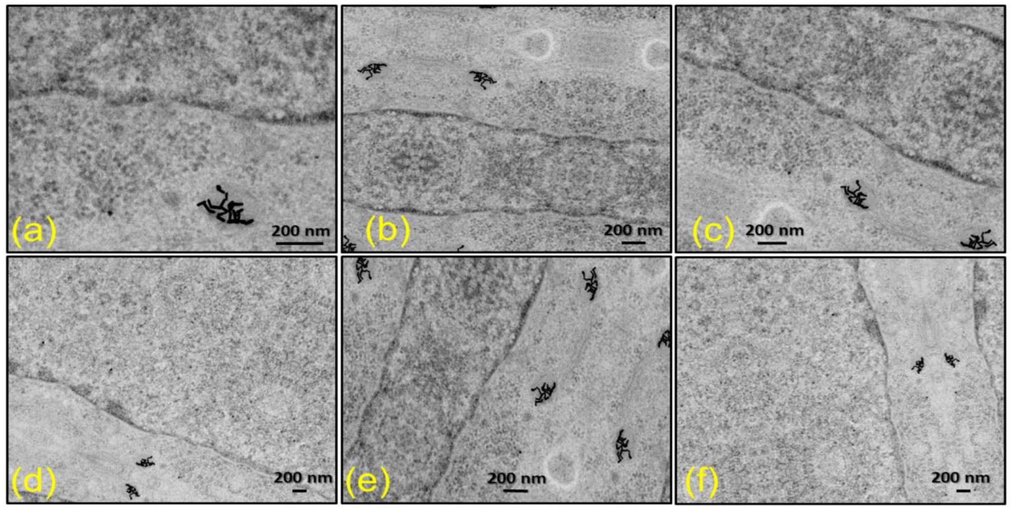
Example of (a) original transmission electron microscopy (TEM) image of human colorectal tumor cells treated with gold nanorods (GNRs) and (b)-(f) augmented TEM images with increased GNR instances. The augmentation techniques applied include rotation, flipping, and scaling to generate diverse training datasets.

CLoDSA (Casado-García et al., 2019) was used in the second data augmentation step. It is also an open-source library that supports many augmentation techniques and allows users to combine them easily. Each image from Dataset1 went through 34 various augmentation steps. The final dataset contained a total of 12040 images (11696 and 344) used to build the model. This was referred to as Dataset2. The number of images, number of available GNPs, and average number of GNP instances per image were all used to divide the original data set. The images were split into three datasets of train, validation, and test sets of 80%/16%/4% using stratified group shuffling technique resulting in 9632, 1926, and 482 train, valid, and test TEM images, respectively, for Dataset2. Similarly, Dataset1 contained 275, 56, and 13 train, valid, and test TEM images, respectively. The training set was used to learn the sample data and estimate the model’s parameters to make it reflect reality and forecast the unknown information. The primary purpose of the validation set was to adjust hyperparameters and evaluate the trained model’s detection capability. A test set was used to assess the trained model’s generalization capability. In our study, two test sets were used for model testing: TestDataSet1 was composed of augmented TEM images, and TestDataSet2 was composed of raw TEM images. The result section provides a detailed explanation of each dataset.

2.2. Model

The YOLO system is based on a single neural network that divides the images’ parts into their respective probability distributions (Redmon et al., 2015). The system then predicts each component’s probability. This works by only looking at one image and making predictions after one forward propagation through the neural network. The object detection algorithm then returns the identified object with non-max suppression. This ensures that each object is only determined once (Redmon et al., 2016). Figure 2 illustrates the basic principle of the YOLO algorithm where Figure 2(a) illustrates the grid division, where the input TEM image is divided into a fixed-size grid (s × s), and each grid cell predicts a certain number of bounding boxes for potential objects. Figure 2(b) shows the bounding box prediction, where the neural network predicts bounding box coordinates, dimensions, and confidence scores for each grid cell, representing the likelihood of an object being present within the bounding box. Figure 2(c) presents the class probability prediction, where the neural network simultaneously predicts class probabilities for each grid cell. In Figure 2(d), the final object detection is depicted. Here, the confidence scores are multiplied by the class probabilities to obtain class-specific confidence scores for each bounding box. Non-maximum suppression (NMS) is then applied to remove overlapping and redundant bounding boxes. The remaining bounding boxes, along with their corresponding class labels and confidence scores, represent the final object detections. The project’s GitHub page (Jocher et al., 2022) contains a detailed overview of the inner structure.

Fig. 2.

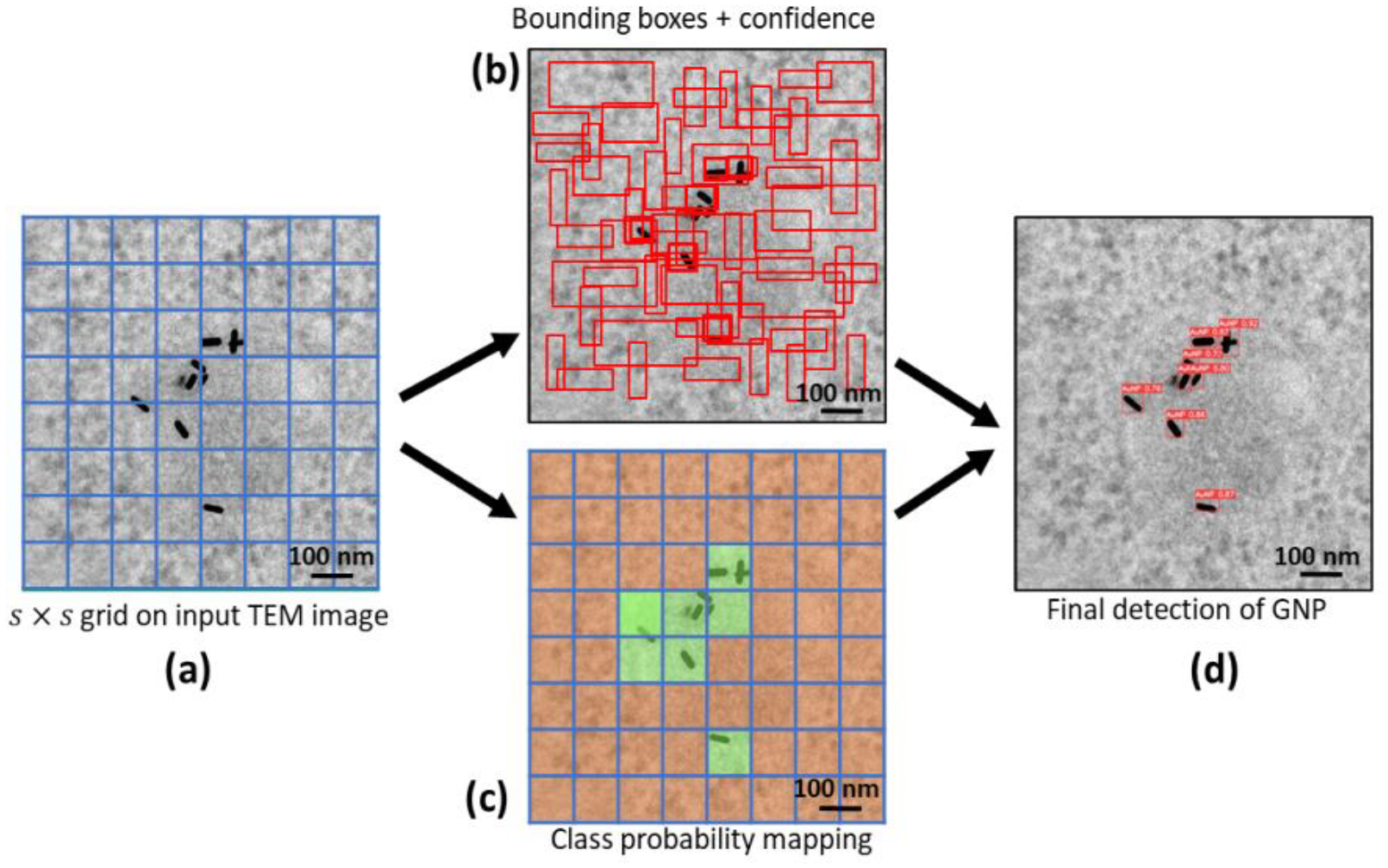
Object detection principle of you only look once (YOLO) algorithm illustrated in four steps: (a) Grid division - Input image (featuring human colorectal tumor cells treated with gold nanorods) divided into a fixed-size grid, with each cell predicting bounding boxes for potential objects. (b) Bounding box prediction - Neural network predicts coordinates, dimensions, and confidence scores for each grid cell, indicating object presence likelihood. (c) Class probability mapping - Neural network concurrently predicts class probabilities for each grid cell, estimating object class likelihood within bounding boxes. (d) Final object detection - Confidence scores are multiplied by class probabilities, and non-maximum suppression (NMS) is applied to remove overlapping and redundant bounding boxes, yielding final gold nanoparticle (GNP) detections.

2.3. Model evaluation metrics

It is essential to create metrics that will allow us to evaluate the performance of DL models after training. In the object detection task, the detection can be either true positive (TP) or false positive (FP) or false negative (FN), or true negative (TN). TP is the number of objects that have been identified successfully. FP is the number of targets that were incorrectly identified. The number of targets not detected is represented by FN. A TN is also a consequence where the model correctly predicts objects of the negative classes. Using these outcomes, we can use the precision (P) and recall (R) to assess the detection capability of the model. These can be calculated using equations (1) and (2).

$$P=\frac{TP}{TP+FP}$$ (1)

$$R=\frac{TP}{TP+FN}$$ (2)

Many object detection models can experience a decline in recall if they are more precise or vice versa. These two numbers can be hard to use for evaluation of the model’s performance. Therefore, the F1 score (as shown in equation 3) is a more straightforward measure that considers precision and recall as the harmonic average. We aim to improve our model by increasing this number. F1 score is calculated when precision and recall are combined, and this score is a number that lies between 0, the worst score, and 1, the best score.

$$F1=2\left(\frac{P\times R}{P+R}\right)$$ (3)

Recall and precision can be mutually exclusive. A model that is accurate and has a high recall as the recall grows will perform superior. In contrast, a model’s performance might be worsened by losing the precision in exchange for the improved recall. Therefore, to measure the trained model’s detection accuracy, the average precision (AP) metric is introduced. Equation (4) defines average precision, and it is the average weight of precisions at each threshold where the increment in recall from the previous threshold determines the weight. In simple language, the area under the precision-recall curve determines the AP value. Higher AP values indicate better prediction accuracy. Multi-class target detection can assess the detection accuracy by computing the average value of all classes of AP, known as mean average precision (mAP), which is described in equation (5).

$$AP=\underset{0}{\overset{1}{\int }}P\left(R\right)dR$$ (4)

$$mAP=\frac{1}{C}\sum _{c=1}^{C}AP\left(c\right)$$ (5)

where C is the number of target categories (our case has only one class of GNP).

We used mAP@0.5, which measures the object detection precision by using the minimum intersection over union (IOU) value greater than or equal to 0.5. We also used another more advanced form of the mAP metric (mAP@0.5–0.95), which calculates the average of all mAP values at IOU levels of 0.5 to 0.95, with a step of 0.05. We aimed to improve the score of mAP@0.5–0.95 and other evaluation metrics. Note YOLOv5 has established a default fitness function as a weighted combination metric in such a way that mAP@0.5 contributes 10%, and mAP@0.50–0.95 contributes the rest.

2.4. Experimental settings

The High-Performance Computing (HPC) research facility at MD Anderson Cancer Center was used for all the model training, utilizing two Tesla V100-SXM2–16GB GPUs with torch 1.11.0+cu102. In addition, all inference tests described in the following sections were carried out using Google Colab Pro computing resources with Tesla T4–16GB GPU. Optimization was performed using the stochastic gradient descent method (SGD). 120 training epochs were used in this study, 16 batches were used for the batch size, 0.01 was used as the initial and final learning rate, 0.005 was used for weight decay, and 0.937 was used for SGD momentum. To accelerate the learning process and conserve computation resources, we used the YOLO’s default pretrained weights. We left the default anchor boxes for the YOLOv5 model at these points: [10,13, 16,30, 33,23] (P3/8), [30,61, 62,45, 59,119] (P4/16) and [116,90, 156,198, 373,326] (P5/32), as defined in the official GitHub repository (Jocher et al., 2022). We experimented with 4 different version of YOLOv5 model named YOLOv5s (small), YOLOv5m (medium), YOLOv5l (large), and YOLO5x (extreme). In addition, we used YOLOv5’s standard data augmentation technique. As far as hyperparameter settings are concerned, they were consistent with the default YOLOv5 settings unless otherwise specified.

3. Results

3.1. Effect of data size

The distribution of GNPs within TEM images is shown in Figure 3. There were 4639 GNP instances in Dataset1. The average number of GNP instances per image was 13.49. On the other hand, there were 159131 GNP cases in Dataset2, and the average number of GNP instances per image was 13.22. Also, it was important to assess the distributions of the widths and heights of the GNP instances in each image. For the 1024×1024 TEM image, normalized average width and height of GNP instances were 0.028±0.025 and 0.028±0.023 pixels, respectively. Their width varied from 0.0023 to 0.3357 pixels and their height from 0.0026 to 0.270 pixels (inset of Figure 3). This demonstrates the irregular morphology of GNPs instances in TEM images concerning size and shape. Similar distributions were observed for Dataset1.

Fig. 3.

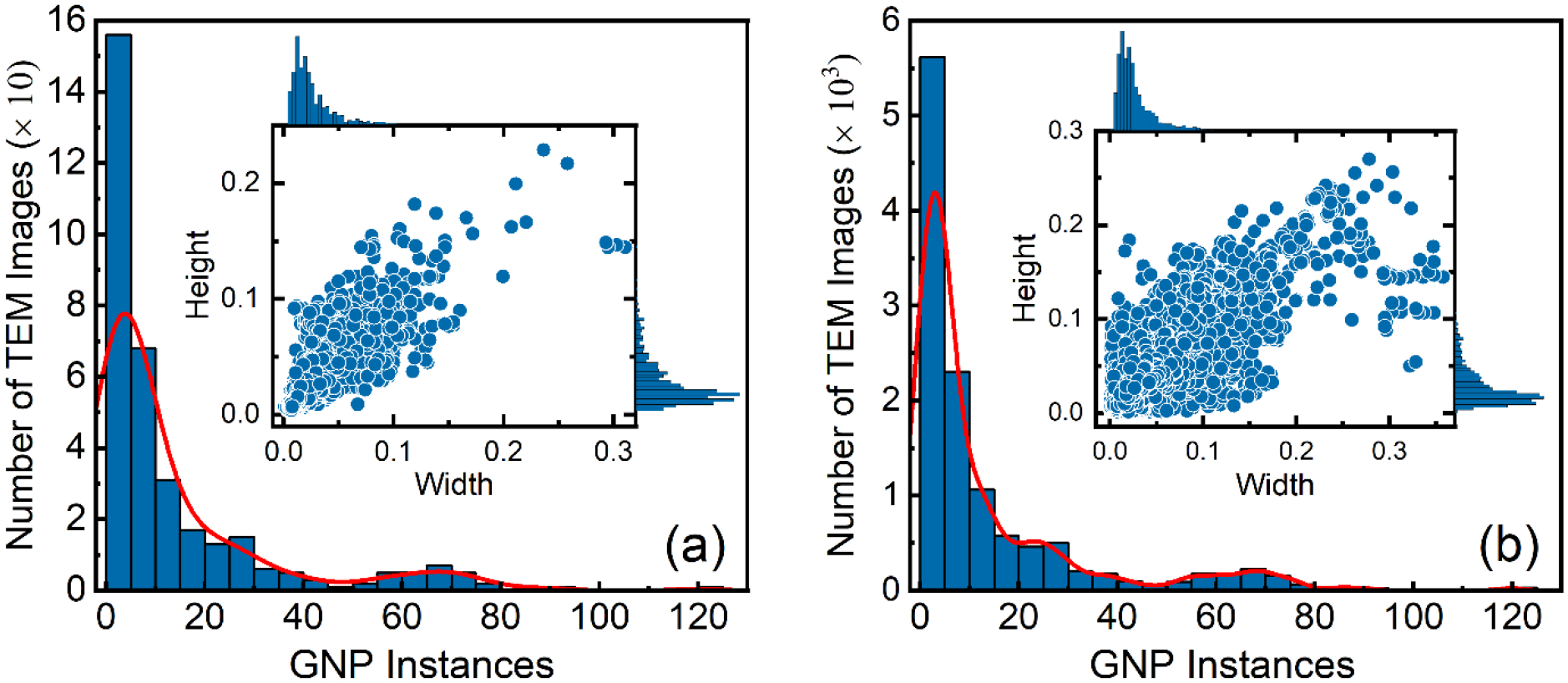
Distribution of gold nanoparticle (GNP) instances in transmission electron microscopy (TEM) images of (a) Dataset1 and (b) Dataset2. Inset shows distribution of normalized widths and heights of GNPs instances. A red line indicates the kernel density distribution of GNP instances, illustrating the concentration and spread of GNPs in the images.

Figure 4 (a–b) illustrates the performance of the same model trained for the same number of epochs and the same initial state of the optimizer. It also shows how different datasets affect the model’s performance. Table 2 showed, Dataset1 had the highest recall score of 0.8498, precision of 0.8756, F1 score of 0.8314, mAP@0.5 of 0.8734, and mAP@0.5–0.95 of 0.4534. Dataset2, on the other hand, achieved maximum recall, precision, F1, mAP@0.5, and the mAP@0.5–0.95 score of 0.9702, 0.9840, 0.9801, 0.9863, and 0.8124, respectively. Compared to Dataset2, the model accuracy of Dataset1 was low because training images in Dataset1 were not sufficient to accurately reflect the characteristics of dataset. We saw that increasing the number of images for training by 35-fold led to an increase in all the evaluation matrices. Dataset1 also showed an overfitting problem because the loss plot indicated a point of inflection (indicated by an arrow in Figure 4 (c–d)). Validation loss must decrease along with training loss to develop DL models. As shown in Figure 4 (c–d), the validation loss increased after 20–30 epochs, while the training loss decreased. Model overfitting occurs when the model has greater control over a small dataset and can satisfy all data points. The network is trying to remember every data point but failing to recognize the general trend of the training dataset. In contrast, Dataset2 had more images, which might decrease the bias in the data. This could help avoid overfitting. In Figure 4 (c–d), both bounding box (bbox) and objectness (obj) loss decrease as the number of epochs increases, which indicates that the YOLOv5l model tends to be more effective. These results demonstrate the importance of data augmentation and show how larger datasets can be used to achieve higher accuracy for CNN models.

Fig. 4.

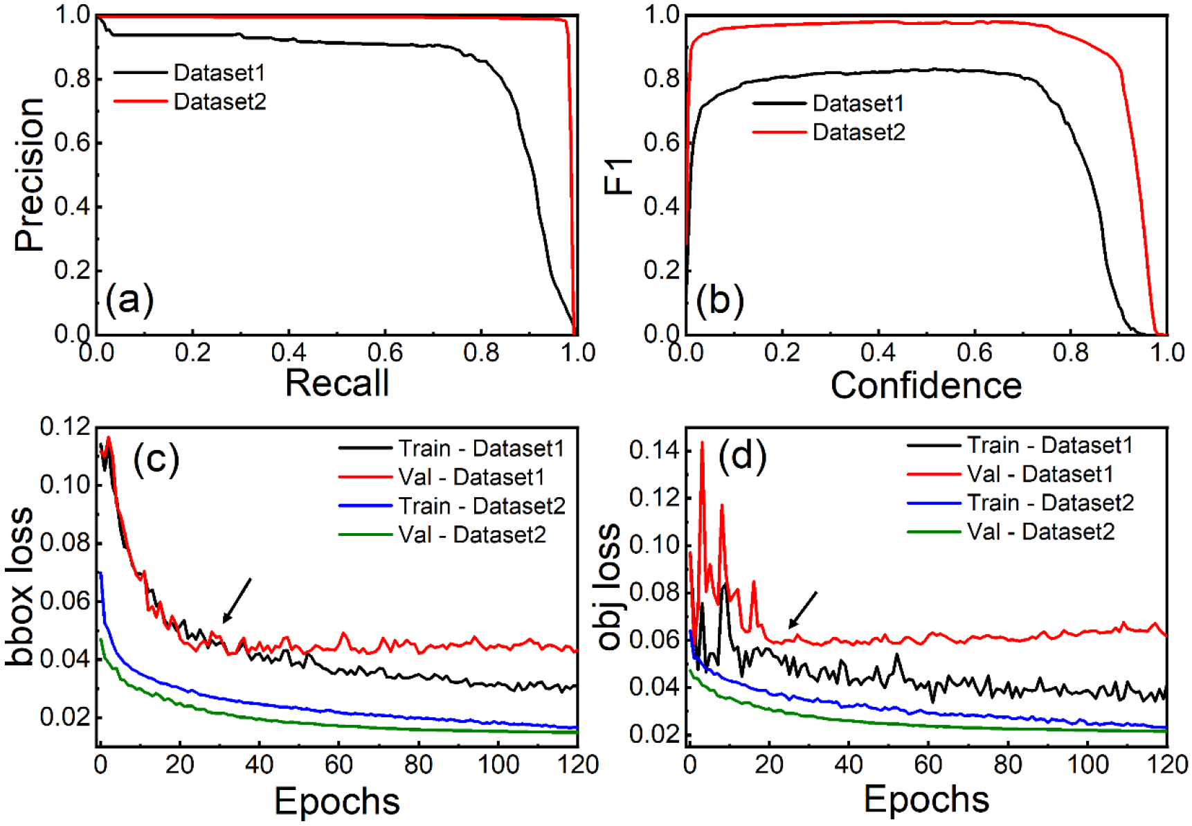
Performance evaluation of the YOLOv5l model trained on two datasets, showcasing (a) precision-recall curve for assessing the trade-off between precision and recall, (b) F1 score plotted against confidence level to determine the optimal confidence threshold, (c) bbox loss plot illustrating the minimization of bounding box prediction errors, and (d) objectness loss plot demonstrating the reduction of object classification errors. Arrows indicate inflection points, highlighting key changes in the plotted metrics.

Table 2.

Comprehensive performance evaluation of the YOLOv5l model across two distinct datasets, showcasing the model’s effectiveness in detecting gold nanoparticles in transmission electron microscopy images.

Datasets	Precision (P)	Recall (R)	F1	mAP@0.50	mAP@0.50–0.95
Dataset1	0.8756	0.8498	0.8314	0.8734	0.4534
Dataset2	0.9840	0.9702	0.9801	0.9863	0.8124

3.2. Comparison of YOLOv5 models

The depth and width of multiple parameters in the model structure can be adjusted according to our needs by utilizing the YOLOv5 model’s setup flexibility. By varying the number of bottlenecks in cross stage partial (CSPs) and the number of convolution cores in each convolution layer, 4 different YOLO models can be obtained, namely YOLOv5s (small), YOLOv5m (medium), YOLOv5l (large), and YOLO5x (extreme) as shown in Table 3. With the expansion of depth and width, so do layers and trainable parameters, and the model becomes more complex.

Table 3.

Comparative analysis of various YOLOv5 model scales, detailing training parameters, results, and computational efficiency. The table includes model depth, width, number of layers, trainable parameters, evaluation metrics (Precision, Recall, F1, mAP@0.5, mAP@0.5–0.95), training time, and inference time per image.

Model	Depth	Width	Number of layers	Trainable parameters	Precision (P)	Recall (R)	F1	mAP@0.5	mAP@0.5–0.95	Training time	Inference time per image
YOLOv5s	0.33	0.50	270	7.0223M	0.9725	0.9493	0.9607	0.9736	0.7360	2h48m54s	0.061 s
YOLOv5m	0.67	0.75	369	20.8713M	0.9809	0.9679	0.9743	0.9844	0.7965	4h7m38s	0.133 s
YOLOv5l	1.00	1.00	468	46.1383M	0.9840	0.9702	0.9770	0.9863	0.8124	6h16m27s	0.202 s
YOLOv5x	1.33	1.25	567	86.2178M	0.9829	0.9744	0.9786	0.9876	0.8157	11h19m12s	0.287 s

Within this section, training metrics are compared, including precision, recall, F1, mAP, loss values, and other criteria that directly impact performance. An overview of the results obtained by various YOLOv5 models is shown in Table 3. The loss function defined in YOLOv3 was also used to calculate the loss value of YOLOv5 (Redmon et al., 2016; Ahmed, 2021). A total loss function was calculated for the YOLOv5 model from regression loss based on bbox loss and obj loss, which was calculated from complete intersection over union loss and binary cross-entropy loss, as well as classification loss (cls loss) (Jocher et al., 2022). We had a single class GNPs, so cls loss was zero in our case. There was a difference in the weighting of the objectness losses across the three prediction layers (P3, P4, P5). Accordingly, the balance weights for small, medium, and large-sized objects were 4, 1, and 0.4. We observed that training losses were slightly higher than validation losses in all cases, possibly due to augmentation during training but absent during validation. As long as the training loss was closest to the validation loss and no inflection point occurred, the model was not overfitting - the lower the loss, the better the model’s accuracy. Therefore, none of the YOLOv5 models was overfitting during the training until epoch 120. We started to see overfitting as validation loss increased and training loss decreased as training further increased. We did not train for more than 120 epochs to avoid overfitting our model. According to Figure 5, the plots of the loss values for all the models share the same characteristics, but the loss value for model x is smaller than those of models l, m, and s. Suppose the evaluation metrics of the four models are compared in Table 3. In that case, it is evident that as the scale of the model increases, recall, F1, and mAP values also rise, resulting in relatively high accuracy. However, for the precision score, model l has the highest precision value of 0.9840, followed by models x, m, and s. Model l and x have extremely comparable mAP@0.5 and mAP @0.5–0.95 values. Also, YOLOv5’ scale growth is evident in Table 3. There is a tendency to increase the training and inference time. When the same number of images are used, the YOLOv5s model spends the shortest training time and makes the fastest predictions. But its accuracy is lowest as compared to other models. To complete 120 epochs training, model x took 11h 19m 12s, but model l required 6h 16m 27s, which was nearly half the time compared to model x. Therefore, our experiments focused on model l for the following few other trials because its training duration was minimal, and the results were nearly identical to model x.

Fig. 5.

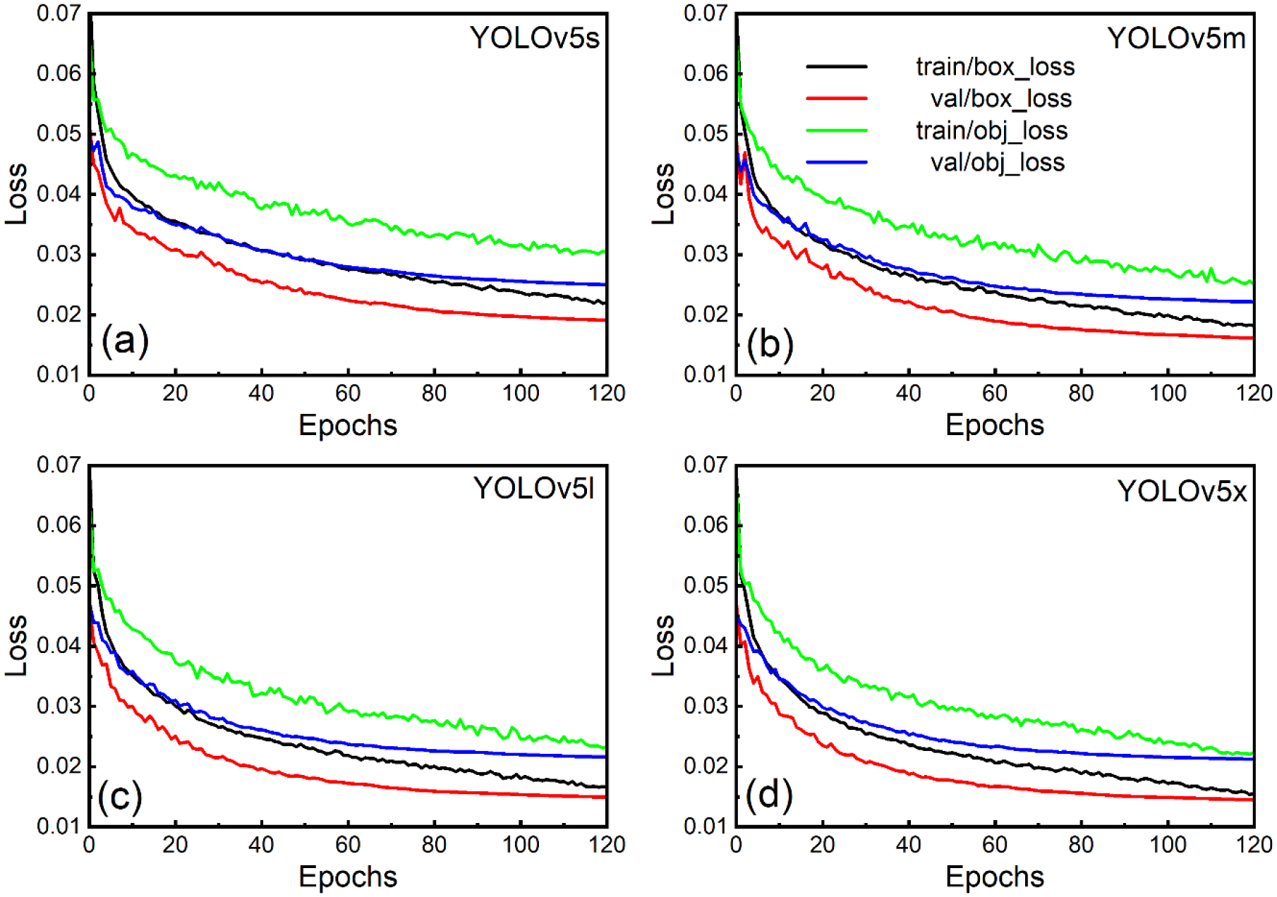
Comparative loss plots for various YOLOv5 model architectures: (a) YOLOv5s (small), (b) YOLOv5m (medium), (c) YOLOv5l (large), and (d) YOLOv5x (extreme). These plots illustrate the training loss progression for each model, providing insights into their convergence and relative performance.

3.3. Transfer learning

Since the original YOLOv5 model was trained on the MS COCO dataset (328K images) (Lin et al., 2014), it can detect objects belonging to 80 different classes. These images contain rich feature representations from a low to a high level. Unfortunately, those 80 classes do not include nanoparticles; hence, without explicit training, the pre-trained model will not be able to identify the nanoparticles from the TEM image dataset. Also, we have a very small number of TEM images, so it is not reasonable to train the YOLOv5 model from scratch with such a small dataset. However, this is an ideal scenario to apply transfer learning. Since the task is the same, i.e., object detection, we can always start with the pre-trained weights on the COCO dataset and then train the model on our images, starting from those initial weights. In this case, the more general aspects of the model are transferred, such as the capability to identify objects by their edges in images. Training is then done on the more specific model layer, which identifies types of objects and shapes. While the model’s parameters will need to be fine-tuned and optimized, its core functionality will have already been determined by transfer learning. Many researchers (Schwarz et al., 2015; Qian et al., 2016; Oquab et al., 2014) have shown that the object detection model can benefit from the transfer learning approach. Therefore, we speculate that our model might also benefit from pre-trained weights. So, we decided to train the model using two strategies: one with pretrained weight and the other from scratch, to see the difference in performance.

Figure 6 shows that the model performed very well when using pre-trained weight for training. The training performance shown in Figure 6 indicates that the model trained with pretrained weight converges fast, because using pre-trained weight keeps the model intuitively from learning basic features. Training and validation bbox and obj loss was low by almost 10–20% for a model trained using pre-trained weight compared to a model trained from scratch. There was an enhancement of 1.13% in precision, 1.08% in the recall, 0.735% in mAP@0.5, and a massive 7.05% in the mAP@0.5–0.95 score. Also, to complete 120 epochs of training, the model from scratch took 6h 41m 51s, and the model with pretrained weight took 6h 16m 27s. Nevertheless, for the model trained from scratch, we obtained the best mAP@0.5–0.95 score of 0.7589 at 120 epochs, whereas to achieve this mAP value, the model with pretrained weight took only 58 epochs just in 3h 1m 36s of training time which was almost half of the training time and epoch took for training from scratch. These results clearly show that training from scratch requires many more epochs, takes more time to train and results are also inferior.

Fig. 6.

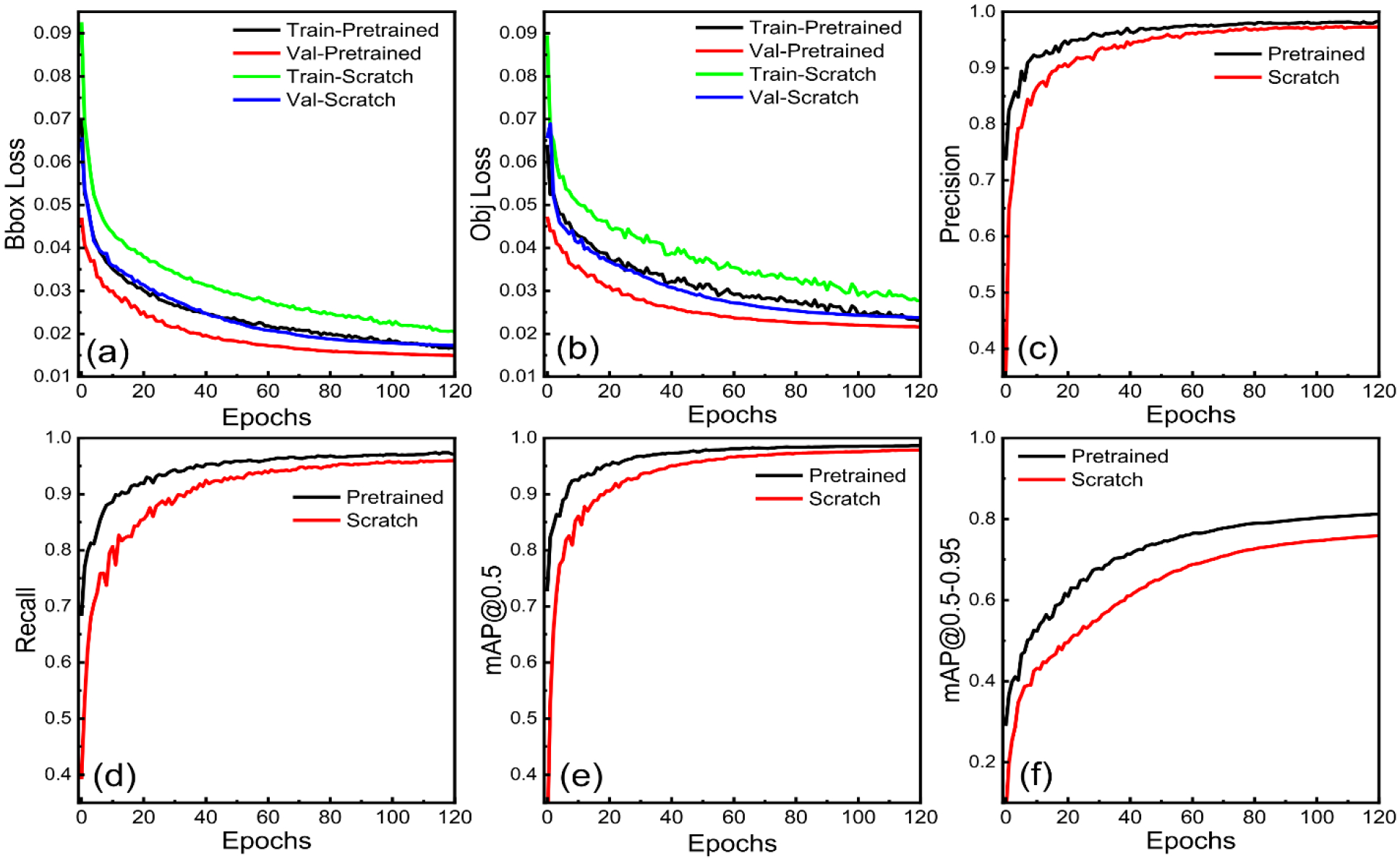
Comparison of YOLOv5l model performance when trained using pre-trained weights versus training from scratch, showcasing the impact of transfer learning on the detection performance. The metrics displayed include: (a) bounding box (bbox) loss, which represents the accuracy of the predicted bounding box coordinates and dimensions, (b) objectness (obj) loss, indicating the model’s ability to correctly identify the presence of objects within bounding boxes, (c) precision, a measure of the proportion of true positive detections among all positive predictions, (d) recall, a measure of the proportion of true positive detections among all actual positives in the dataset, (e) mean average precision (mAP) at intersection over union (IoU) threshold of 0.5, representing the model’s overall detection performance, and (f) mAP at IoU thresholds ranging from 0.5 to 0.95, providing a more comprehensive evaluation of the model’s performance across various IoU thresholds.

3.4. Image size comparison

We experimented with various input image sizes to see how resizing affects the model’s performance. The input images were scaled up or down according to the resolution, with the lowest image resolution being 340×340 and the highest image resolution being 1280×1280. For this experiment, we used a batch size of 32 for an input image size of 320, 512, and 640, a batch size of 24 for 800, and 16 for 1024 and 1280, respectively. As the image was scaled to different pixel sizes, the object in the images also changed. The best part of the YOLOv5 model is that the annotation information in the dataset is checked before the start of training and calculates the optimal recall rate for the dataset annotation information for the default anchor box. It uses the default anchor box when the optimal recall rate is greater than or equal to 0.98. If the optimal recall rate is less than 0.5% of 0.98, new anchors are automatically computed, evolved, and attached to the model. It uses a genetic evolution optimizer (Goldberg, 1988) on the anchors following a k-means scan. For an image size of 320, default anchors were likely a poor fit for our dataset. So, it recalculated the new anchor boxes of [3,3, 5,5, 7,7], [10,9, 13,13, 15,23] and [25,17, 29,29, 54,45]. Similarly, for image size of 512, default anchor boxes changed to [4,4, 6,6, 9,9], [12,12, 18,18, 20,28] and [33,24, 42,43, 100,92]. For all other image size, default anchor boxes of [10,13, 16,30, 33,23], [30,61, 62,45, 59,119] and [116,90, 156,198, 373,326] were good fit.

Due to the presence of small nanoparticles in the input image, the image’s dimensions significantly influenced the model’s mAP, F1, precision, and recall score (Figure 7(a)). Our model’s mAP@0.5–0.95 increased from 0.6634 to 0.8231 as image resolution increased from 340 to 1280, a 24.09% improvement. Similarly, there was an enhancement of 9.19% in mAP@0.5, 16.93% in Recall, and 2.13% in precision, respectively. These findings were validated by the results shown in Figure 7(b), which indicate that the bbox loss decreased for the higher resolution images. It is believed that objectness loss is compromised by a highly imbalanced sample set between positive and negative. When an image is scaled up, the object count inside images remains the same, increasing the imbalance. Therefore, the loss gain is automatically scaled to the image size of 640 in the YOLOv5 model to compensate for this effect. Consequently, as image size increases, obj loss decreases up to 640 and then increases. In general, expanding the sizes of the images tends to increase the time required to finish each epoch, as expected. This varied from 1m 7s for the smallest image size of 320×320 to 4m 55s for the largest image size of 1280×1280. It can be concluded that when the image resolution is high, the model performance is better; however, the training is computationally expensive because GPU memory utilization rises as image size increases due to an increase in the number of trainable parameters and neurons in convolution and fully connected layers. We concluded that when dealing with tiny nanoparticles of small pixel size, it is crucial to train the model on the native high resolution to improve the abundance of characteristics. Then the trained model can correctly detect and identify the nanoparticles from the cell by doing so.

Fig. 7.

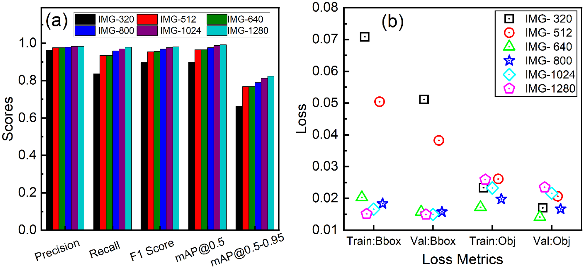
Performance evaluation of the YOLOv5l model with varying transmission electron microscopy (TEM) image sizes to assess the impact of image resolution on detection accuracy: (a) evaluation metrics, including precision, recall, F1 score, and mean average precision (mAP) at different intersection over union (IoU) thresholds, providing a comprehensive understanding of the model’s performance for each image size, and (b) loss plot, illustrating the convergence and training stability for different image resolutions. The numbers listed from 320 to 1280 denote the pixel dimensions of the images; for instance, IMG-320 corresponds to TEM images with a 320×320-pixel resolution.

3.5. Progressive image resizing

Progressive image resizing is a method of resizing all images in order while training DL algorithms on smaller to larger image sizes. Many researchers (Colangelo et al., 2021; Bhatt et al., 2021; Farooq & Hafeez, 2020) have shown that progressive resizing methods improve the performance of the DL model. Each larger-scale model includes the preceding smaller-scale model layers and weights into its architecture, fine-tuning the final model and boosting the accuracy score (Howard & Gugger, 2020). Progressive resizing has another advantage: it is a type of data augmentation. As a result, we should expect improved generalization from models trained with progressive image resizing. Therefore, we applied this strategy to train the YOLOv5l model with a smaller image size of 512×512 for 100 epochs and then used the weights from the first model to train another second model with an image size of 800×800 for 100 epochs. Further, we used the weights from the second model to train the third model on images of size of 1024×1024 for another 100 epochs.

Figure 8(a) shows the enhancement in all evaluation matrices by progressive image resizing methods. Improvement was 0.82% for precision, 0.61% for recall, 0.68% for F1 score, 0.38% for mAP@0.5, and 5.01% for mAP@0.5–0.95. Overall, the models’ mAP@0.5–0.95 was significantly improved, proving that progressive image resizing helped us get better results. On the other hand, even with the good result on the accuracy, the progressive resizing technique took more training time than the normal training; it was almost two times longer (10h 59m 52s) than the normal training time (5h 13m 35s) for 100 epochs. Although training by this approach required high computational effort and energy requirements, it was worth training because the model’s mAP could be improved by 5%.

Fig. 8.

(a) Effect of progressive image resizing on YOLOv5l model performance, illustrating the percentage improvements in all evaluation metrices; (b) precision-recall curve for our best-performing YOLOv5l model, illustrating the trade-off between precision and recall in detecting gold nanoparticles in two different test datasets, providing insights into the overall detection performance and suitability of the model for practical applications; and (c) F1 score as a function of confidence level for the two test datasets, demonstrating the optimal confidence threshold for maximizing the balance between precision and recall.

3.6. Detection and performance results on test dataset

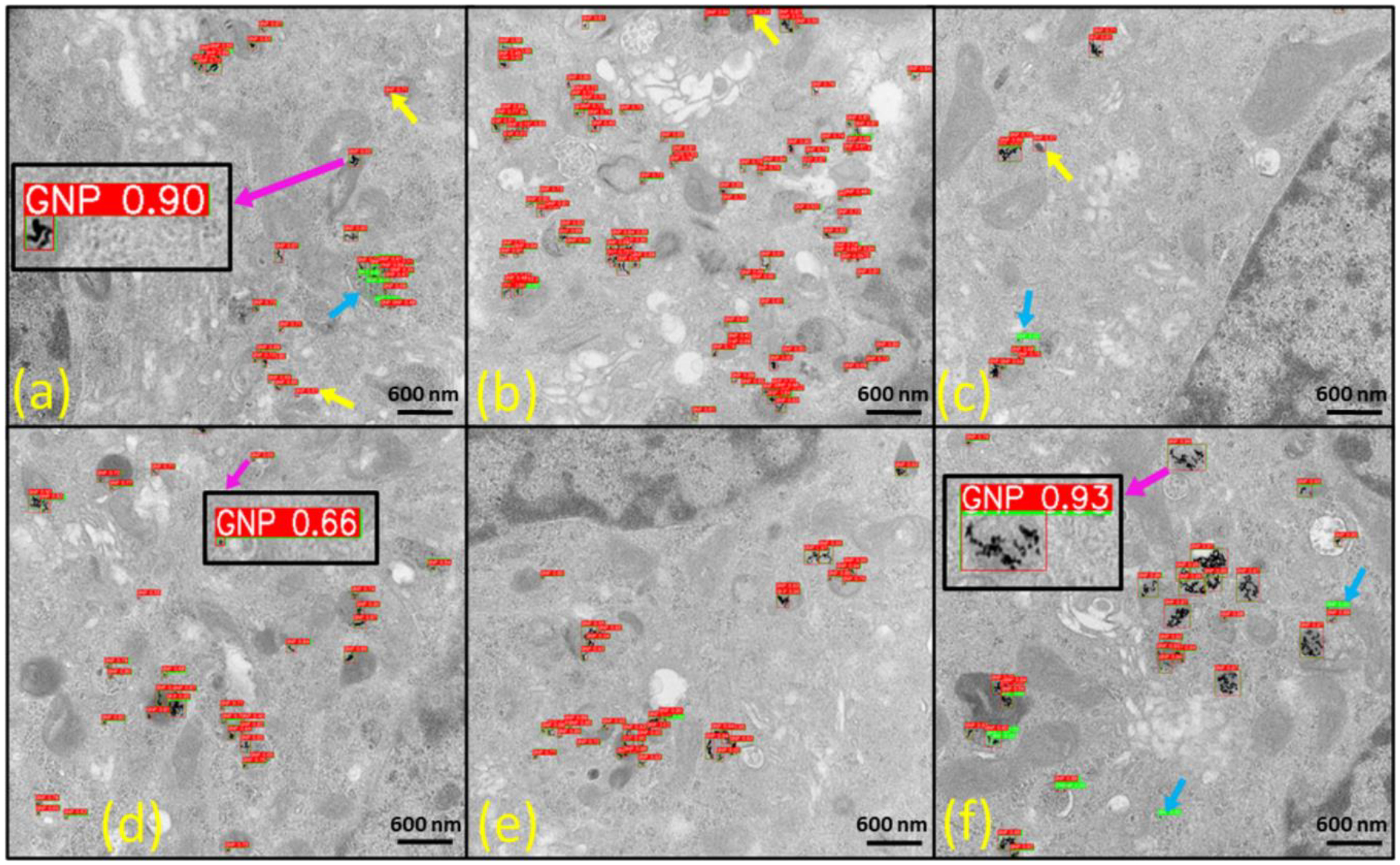
To provide an unbiased evaluation of the final model fit on the training dataset, we compared detection results obtained on two separate test data sets: TestDataSet1 and TestDataSet2. 482 TEM images were presented in TestDataSet1, and 7811 ground truth labels were generated using various augmentation techniques. TestDataSet2, however, contained 36 raw TEM images along with 456 ground truth labels. Figure 8 (b–c) illustrates the performance of the trained YOLOv5l model on two test datasets.

We analyzed the performance and evaluated the predictions based on the ground truth data. Some examples of our best model prediction on the more complex TestDataSet2 are shown in Figure 9 and Figure 10. The best model we developed generated 7787 prediction structures for TestDataSet1. Out of these predictions, 7639 predictions were TPs, 148 predictions were FPs, and 24 were FNs. Using these values, we estimated a precision of 0.981, a recall of 0.978, and an F1 score of 0.978 at a confidence interval of 0.624. In contrast, our best model for TestDataSet2 produced 446 predictions, with 417 TPs, 29 FPs, and 10 FNs, yielding a precision of 0.935, a recall of 0.914, and an F1 score of 0.925 at a confidence level of 0.417. Accordingly, mAP@0.5 for TestDataSet1 and TestDataSet2 was 0.99 and 0.95, respectively. The TEM images without GNPs in TestDataSet1 and TestDataSet2 were 74 and 6, respectively. Our model accurately predicted that there was no GNPs in those images. This proves that our model could distinguish the background cellular structures very well. Even though there was a slight decline in the performance of the detection algorithm on the TestDataSet2 that only contained raw TEM images, given that the TestDataSet2 contained much more complex images, the performance was still very high (≈95%). There were a few false positive and false negative results in our models as shown by yellow and light blue arrows in Figure 9 and Figure 10. The results demonstrated that the YOLOv5 model could efficiently acquire adequate information from the training image sets to identify GNPs from a cellular image correctly.

Fig. 9.

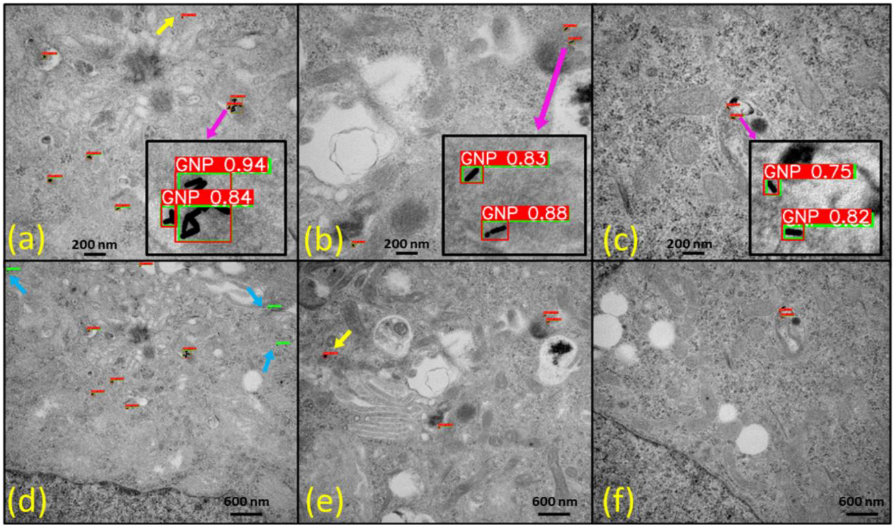
Detection results of our best YOLOv5l model on TestDataSet2 featuring human colorectal tumor cells treated with cylindrical gold nanoparticles (GNPs), i.e., gold nanorods (10 nm diameter and 40 nm length). (a)-(c) raw transmission electron microscopy (TEM) images at 50000 magnification and (d)-(f) raw TEM images at 25000 magnifications. The yellow arrow indicates false-positive results, while the light blue arrow highlights false-negative results. Insets display zoomed-in images of GNPs, revealing the confidence scores associated with each detection. The red bounding boxes represent the detection results, and the green bounding boxes denote ground-truth labels, providing a clear visual comparison of model predictions and actual GNP locations within the TEM images.

Fig. 10.

Detection results of our best YOLOv5l model on TestDataSet2 featuring human pancreatic tumor cells treated with spherical gold nanoparticles (GNPs), i.e., gold nanospheres of 5 nm diameter. All raw TEM images are at 25000 magnifications. The yellow arrow indicates false-positive results, while the light blue arrow highlights false-negative results. Insets display zoomed-in images of GNPs, revealing the confidence scores associated with each detection. The red bounding boxes represent the detection results, and the green bounding boxes denote ground-truth labels, providing a clear visual comparison of model predictions and actual GNP locations within the TEM images.

Because we trained our model with the 1024×1024-pixel image size, for the best detection performance, the inference must also be performed with the exact resolution; however, YOLOv5 can be inferred from any resolution image. Consequently, more precise detection is a challenge for large-scale input images when the object is very tiny, like GNPs in our case. The image can be randomly cropped or resized, but this approach is obviously not viable for inference since information may be lost while resizing to a lower resolution. Slicing-Assisted Hyper Inference (SAHI) (Akyon et al., 2022) is of use in this case. In SAHI, slices predictions take the input image, break it down into slightly overlapping patches, perform predictions on each patch, and then combine the annotated patches to visualize them on the original image. We applied this approach to our TEM images of GNRs whose native resolution was 2256×2048. Since our model was trained at 1024×1024 images, we used slice height and width of 1024, the detection confidence level of 0.42, and the overlap ratio of 0.2. Figure 11 clearly shows that the SAHI prediction technique enabled the detection of solitary GNPs that were missed by normal inference. As a result, it removed some false detection making our detection algorithm more precise. However, SAHI prediction took slightly more inference time (0.34s per image) than standard inference time (0.20s per image). This result shows the advantage of SAHI prediction if the detection image resolution is higher than the training image size.

Fig. 11.

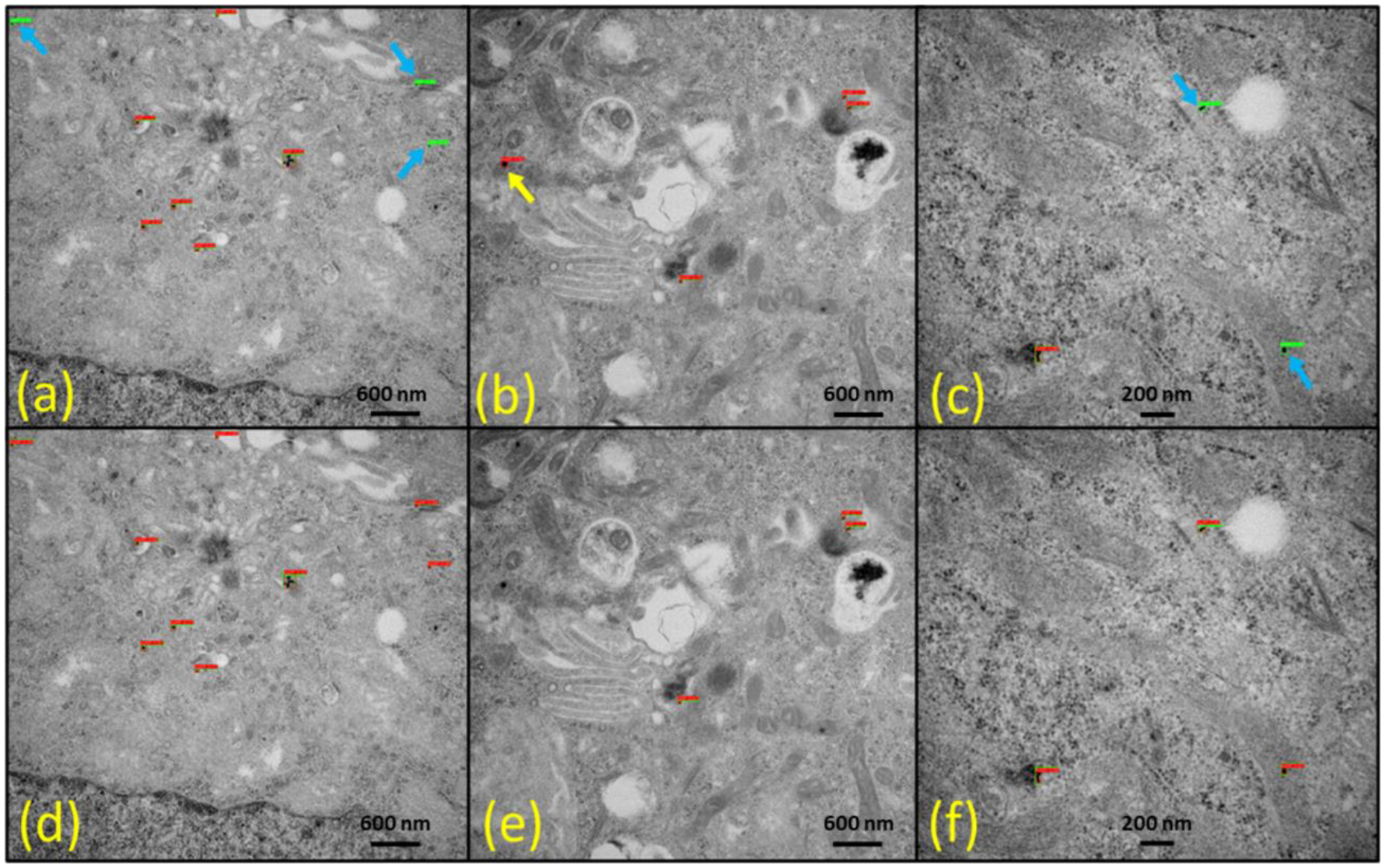
Detection results using standard inference (a-c) and Slicing-Assisted Hyper Inference (SAHI) prediction (d-f) on raw transmission electron microscopy (TEM) images featuring human colorectal tumor cells treated with cylindrical gold nanoparticles (GNPs) (i.e., gold nanorods). The yellow arrow highlights false-positive results, while the light blue arrow points out false-negative results. The red bounding boxes represent the detection results, and the green bounding boxes denote the ground-truth labels, showcasing the effectiveness of each method in identifying GNPs within the TEM images.

4. Discussion

This study aimed to develop a reliable and fully automated method for detecting nanoparticles (specifically GNPs within the current scope) in cellular TEM images. Manual detection of nanoparticles can be very time consuming and may even be considered impractical in many cases. The DL model developed from this study automatically recognizes nanoparticles and does not require an annotation by a human. To our knowledge, no prior study has demonstrated these capabilities. After training based only on a few TEM images, we analyzed heterogeneous cellular TEM images with higher accuracy. Importantly, data from the YOLOv5 model allowed us to precisely estimate the number and position of nanoparticles within cell structures.

Four different architectures of YOLOv5 models were tested, YOLOv5s, YOLOv5m, YOLOv5l, and YOLOv5x. As we moved from a small model to an extreme one, there was a tendency for the inference and training time to increase. The YOLOv5s model took the shortest time to train and made the fastest predictions, even though it used the same number of images. However, its accuracy was lower than other models. We found that both the YOLOv5l object detectors and YOLOv5x object detectors were suitable for this task. They both had an equivalent mAP value. The model also performed well when it was trained with pre-trained weight. The pre-trained weight helped the model to learn basic features faster, which is evident in the model’s training performance. Our study also showed that models performed better when images were high quality for training. However, training was computationally costly because GPU memory usage rose with increasing image sizes due to an increase in trainable parameters. We found that increasing the image resolution for TEM images was the key to enhancing the sensitivity of nanoparticle detection. Nanoparticles in cells could then be better detected and distinguished using the trained model. Two of the most popular deep network optimization algorithms, Adam (result not shown here) and SGD, were also tested. We concluded that, SGD might be an excellent choice for object detection models, as there was a performance gap with Adam when used default hyperparameters. Our results also revealed that progressive image resizing methods improved all evaluation matrices of models. Although this approach was time-consuming and expensive, it was also able to enhance the model’s mAP by 5%. Besides, our model was able to handle nanoparticle detection from TEM image sets with multi-magnification, as shown in Figure 9.

The YOLOv5 trained model was able to produce predictions from raw TEM images that outperformed human detection. Manually counting and locating each TEM image of approximately 10 GNPs took around 2–3 minutes for an expert technician. However, on average, our YOLOv5 model processed 1 TEM image containing any number of GNPs and generated predictions in just 0.2s using a single GPU. This was almost a 900-fold increase in speed, reducing effort and time. Besides, it did not necessitate a lot of computational resources, as 10–12 hours of training time were sufficient for the results obtained. The YOLOv5 algorithm is very scalable for large datasets. This can be seen by the short training time required for our dataset. We expect that the current approach can be extended beyond the detection of GNPs within cells using TEM image for biomedical applications. For example, it can also be used to analyze typical TEM images of nanoparticles in materials science.

To demonstrate the robustness and reliability of our approach, we used a more complex dataset that included GNPs in general and controlled environments. Next, we selected samples with noisy backgrounds and added more noise manually which looked like GNPs, and then performed detection using our trained model. Some detection results can be seen in Figure 12. There were few false-negative detections of solitary tiny GNPs; however, we observed no false positive detection. Likewise, we selected sample images containing solitary GNPs from the test dataset to verify that the proposed algorithm was able to accurately detect these particles. This test showed that our YOLOv5 model correctly detected smaller GNPs in the input images. Although there were few missed detections of solitary GNPs, it was able to identify clustered GNPs more accurately, which could be crucial for modeling of GNP-mediated dose enhancement & radiosensitization (Jayarathna et al., 2019).

Fig. 12.

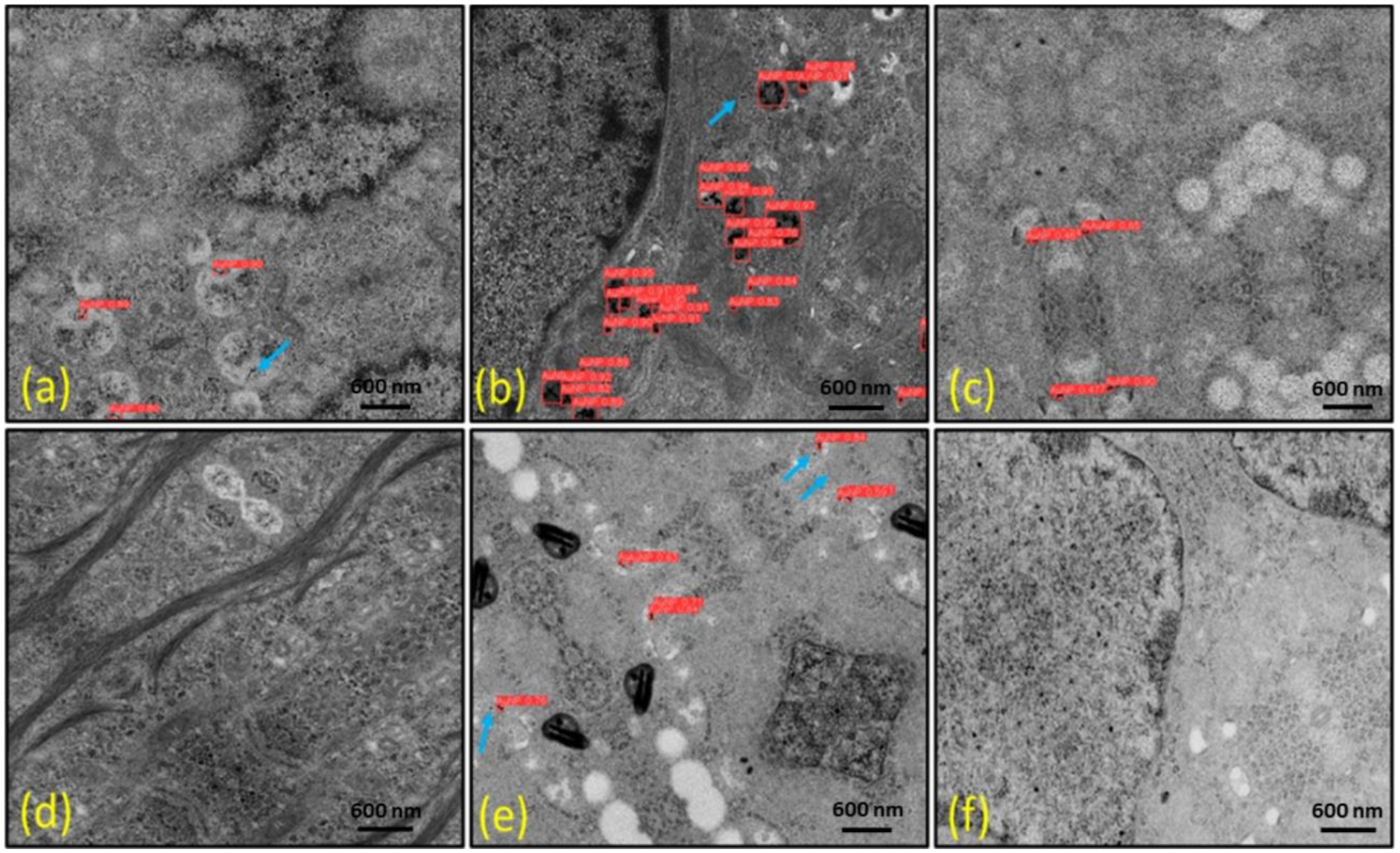
Detection of gold nanoparticles (GNPs) on noisy cellular backgrounds featuring augmented images with added noise to test the model’s robustness. (a, c, e) show colorectal tumor cells, while (b, d, f) represent pancreatic tumor cells. The light blue arrow highlights false-negative results. Notably, there are no GNPs present in (d) and (f), and our model accurately distinguishes background cellular structures from GNPs, demonstrating its ability to perform effectively under challenging, noisy conditions.

The relatively small training dataset was one of the challenges of this study. Although we used augmented images to train the model, it could have been more accurate if we had access to a larger number of datasets. Our model struggled to detect tiny solitary GNPs in a few cases. Since our ultimate goal within the current scope is to study GNP-mediated dose enhancement & radiosensitization, however, the possibility of missing a few GNPs out of hundreds could be insignificant. Even so, the DL model developed from this investigation can be trained with an expanded image dataset to achieve even better detection performance and a shorter computational time.

While not demonstrated in this investigation, the currently developed DL-based TEM image analysis tool can, in principle, be extended for the detection of other internalized metal nanoparticles (MNPs) (e.g., made of iron, hafnium, gadolinium, etc.) that have also been considered for cancer treatments and diagnosis. The current approach is also expected to be independent of specific TEM imaging devices. Furthermore, it may serve as the basis for the development of other related tools that can help facilitate computational modeling of GNP- or MNP-laden tumor cells. For example, following the detection of GNPs and MNPs, it is possible to automatically determine other important modeling parameters such as the distances between internalized GNPs and MNPs and specific subcellular organelles (e.g., nuclei and mitochondria). Given the impracticality of a manual determination of such parameters, the benefits from this possibility are easily foreseeable.

5. Conclusion

We employed a DL-based YOLOv5 model for detecting GNPs in cellular TEM images. The robustness and reliability of our method were demonstrated by analyzing a more complex dataset involving GNPs in general and controlled environments. In a validation set, our best model achieved maximum recall, precision, F1, mAP@0.5, and mAP@0.5–0.95 scores of 0.987, 0.976, 0.982, 0.989, and 0.843, respectively. The trained model performed very well on a complex raw test dataset with a precision of 93.5%, a recall of 91.4%, an F1 score of 92.5%, and mAP@0.5 of 95.0% at a confidence level of 0.417. Utilizing the currently developed method, the time required for hundreds of TEM image analyses can be reduced from hours to less than a minute. Furthermore, our proposed method has high repeatability since it is operator independent. Overall, we have shown that the YOLOv5 model allows for precise determination of GNP distributions throughout cellular structures. This enables us to fully automate GNP detection from cellular TEM images, successfully addressing the key challenge for the development of nanometer resolution TEM image-based models of GNP-laden cells. Owing to its generality, the current DL-based approach can also be extended for the detection of other MNPs, besides GNPs, considered for cancer diagnostic and therapeutic applications.

References

- Ahmed KR (2021). Smart Pothole Detection Using Deep Learning Based on Dilated Convolution. Sensors 21, 8406. 10.3390/s21248406 (Accessed April 26, 2022). [DOI] [PMC free article] [PubMed] [Google Scholar]
- Akyon FC, Altinuc SO & Temizel A (2022). Slicing Aided Hyper Inference and Fine-tuning for Small Object Detection. 10.48550/arXiv.2202.06934 (Accessed May 11, 2022). [DOI] [Google Scholar]
- Azam MA, Sampieri C, Ioppi A, Africano S, Vallin A, Mocellin D, Fragale M, Guastini L, Moccia S, Piazza C, Mattos LS & Peretti G (2022). Deep Learning Applied to White Light and Narrow Band Imaging Videolaryngoscopy: Toward Real‐Time Laryngeal Cancer Detection. The Laryngoscope 132, 1798–1806. 10.1002/lary.29960 (Accessed May 8, 2022). [DOI] [PMC free article] [PubMed] [Google Scholar]
- Bhatt AR, Ganatra A & Kotecha K (2021). Cervical cancer detection in pap smear whole slide images using convNet with transfer learning and progressive resizing. PeerJ Computer Science 7, e348. 10.7717/peerj-cs.348 (Accessed May 4, 2022). [DOI] [PMC free article] [PubMed] [Google Scholar]
- Bochkovskiy A, Wang C-Y & Liao H-YM (2020). YOLOv4: Optimal Speed and Accuracy of Object Detection. 10.48550/arXiv.2004.10934 (Accessed May 3, 2022). [DOI] [Google Scholar]
- de Boodt S, Poursaberi A, Schrooten J, Berckmans D & Aerts J-M (2013). A semiautomatic cell counting tool for quantitative imaging of tissue engineering scaffolds. Tissue engineering. Part C, Methods 19, 697–707. 10.1089/ten.tec.2012.0486 (Accessed May 8, 2022). [DOI] [PubMed] [Google Scholar]
- Carnovale C, Bryant G, Shukla R & Bansal V (2019). Identifying Trends in Gold Nanoparticle Toxicity and Uptake: Size, Shape, Capping Ligand, and Biological Corona. ACS Omega 4, 242–256. 10.1021/acsomega.8b03227 (Accessed May 17, 2022). [DOI] [Google Scholar]
- Casado-García Á, Domínguez C, García-Domínguez M, Heras J, Inés A, Mata E & Pascual V (2019). Clodsa: A tool for augmentation in classification, localization, detection, semantic segmentation and instance segmentation tasks. BMC Bioinformatics 20, 1–14. 10.1186/s12859-019-2931-1 (Accessed May 3, 2022). [DOI] [PMC free article] [PubMed] [Google Scholar]
- Chen H-H, Chien C-C, Petibois C, Wang C-L, Chu YS, Lai S-F, Hua T-E, Chen Y-Y, Cai X, Kempson IM, Hwu Y & Margaritondo G (2011). Quantitative analysis of nanoparticle internalization in mammalian cells by high resolution X-ray microscopy. Journal of nanobiotechnology 9, 14. 10.1186/1477-3155-9-14 (Accessed May 8, 2022). [DOI] [PMC free article] [PubMed] [Google Scholar]
- Chithrani BD, Ghazani AA & Chan WCW (2006). Determining the size and shape dependence of gold nanoparticle uptake into mammalian cells. Nano Letters 6, 662–668. 10.1021/nl052396o (Accessed May 8, 2022). [DOI] [PubMed] [Google Scholar]
- Colangelo F, Battisti F & Neri A (2021). Progressive Training Of Convolutional Neural Networks For Acoustic Events Classification. In 2020 28th European Signal Processing Conference (EUSIPCO), pp. 26–30. IEEE; 10.23919/Eusipco47968.2020.9287362 (Accessed May 4, 2022). [DOI] [Google Scholar]
- Farooq M & Hafeez A (2020). COVID-ResNet: A Deep Learning Framework for Screening of COVID19 from Radiographs. 10.48550/arXiv.2003.14395 (Accessed May 4, 2022). [DOI] [Google Scholar]
- Girshick R (2015). Fast R-CNN. In 2015 IEEE International Conference on Computer Vision (ICCV), pp. 1440–1448. IEEE; 10.1109/ICCV.2015.169. [DOI] [Google Scholar]
- Girshick R, Donahue J, Darrell T & Malik J (2013). Rich feature hierarchies for accurate object detection and semantic segmentation. 10.48550/arXiv.1311.2524 (Accessed May 8, 2022). [DOI] [Google Scholar]
- Goldberg DE (1988). Genetic algorithms in search, optimization, and machine learning. American Library Association; 10.5860/choice.27-0936 (Accessed May 3, 2022). [DOI] [Google Scholar]
- Groschner CK, Choi C & Scott MC (2021). Machine Learning Pipeline for Segmentation and Defect Identification from High-Resolution Transmission Electron Microscopy Data. Microscopy and Microanalysis 27, 549–556. [DOI] [PubMed] [Google Scholar]
- Hainfeld JF, Slatkin DN & Smilowitz HM (2004). The use of gold nanoparticles to enhance radiotherapy in mice. Physics in Medicine and Biology 49, N309–N315. 10.1088/0031-9155/49/18/N03 (Accessed May 19, 2022). [DOI] [PubMed] [Google Scholar]
- Hao Y, Yang X, Song S, Huang M, He C, Cui M & Chen J (2012). Exploring the cell uptake mechanism of phospholipid and polyethylene glycol coated gold nanoparticles. Nanotechnology 23, 045103. 10.1088/0957-4484/23/4/045103 (Accessed May 8, 2022). [DOI] [PubMed] [Google Scholar]
- He K, Gkioxari G, Dollár P & Girshick R (2017). Mask R-CNN. 10.48550/arXiv.1703.06870 (Accessed May 8, 2022). [DOI] [PubMed] [Google Scholar]
- He K, Zhang X, Ren S & Sun J (2015). Spatial Pyramid Pooling in Deep Convolutional Networks for Visual Recognition. IEEE Transactions on Pattern Analysis and Machine Intelligence 37, 1904–1916. 10.1109/TPAMI.2015.2389824 (Accessed May 8, 2022). [DOI] [PubMed] [Google Scholar]
- Howard J & Gugger S (2020). Deep Learning for Coders with Fastai and Pytorch. O’Reilly Media, Inc. [Google Scholar]
- Ito E, Sato T, Sano D, Utagawa E & Kato T (2018). Virus Particle Detection by Convolutional Neural Network in Transmission Electron Microscopy Images. Food and Environmental Virology 10, 201–208. 10.1007/s12560-018-9335-7 (Accessed May 8, 2022). [DOI] [PubMed] [Google Scholar]
- Jain S, Hirst DG & O’Sullivan JM (2012). Gold nanoparticles as novel agents for cancer therapy. The British Journal of Radiology 85, 101. /pmc/articles/PMC3473940/ (Accessed September 20, 2022). [DOI] [PMC free article] [PubMed] [Google Scholar]
- Jayarathna S, Manohar N, Ahmed MF, Krishnan S & Cho SH (2019). Evaluation of dose point kernel rescaling methods for nanoscale dose estimation around gold nanoparticles using Geant4 Monte Carlo simulations. Scientific Reports 9, 3583. 10.1038/s41598-019-40166-9 (Accessed August 7, 2022). [DOI] [PMC free article] [PubMed] [Google Scholar]
- Jocher G, Chaurasia A, Stoken A, Borovec J, NanoCode012, Kwon Y, TaoXie, Fang J, imyhxy, Michael K, Lorna V,A, Montes D, Nadar J, Laughing, tkianai, yxNONG, Skalski P, Wang Z, Hogan A, Fati C, Mammana L, AlexWang1900, Patel D, Yiwei D, You F, Hajek J, Diaconu L & Minh MT (2022). ultralytics/yolov5: v6.1 - TensorRT, TensorFlow Edge TPU and OpenVINO Export and Inference. 10.5281/zenodo.6222936 (Accessed April 26, 2022). [DOI] [Google Scholar]
- Kapur JN, Sahoo PK & Wong AKC (1985). A new method for gray-level picture thresholding using the entropy of the histogram. Computer Vision, Graphics, and Image Processing 29, 273–285. 10.1016/0734-189X(85)90125-2 (Accessed May 8, 2022). [DOI] [Google Scholar]
- Kim JA, Åberg C, Salvati A & Dawson KA (2012). Role of cell cycle on the cellular uptake and dilution of nanoparticles in a cell population. Nature Nanotechnology 7, 62–68. 10.1038/nnano.2011.191 (Accessed May 8, 2022). [DOI] [PubMed] [Google Scholar]
- Lin TY, Goyal P, Girshick R, He K & Dollar P (2017). Focal Loss for Dense Object Detection. 318–327. 10.48550/arXiv.1708.02002 (Accessed May 8, 2022). [DOI] [PubMed] [Google Scholar]
- Lin T-Y, Maire M, Belongie S, Hays J, Perona P, Ramanan D, Dollár P & Zitnick CL (2014). Microsoft COCO: Common Objects in Context. In Computer Vision – ECCV 2014. Springer, Cham: 10.1007/978-3-319-10602-1_48 (Accessed May 2, 2022). [DOI] [Google Scholar]
- Liu W, Anguelov D, Erhan D, Szegedy C, Reed S, Fu C-Y & Berg AC (2016). SSD: Single Shot MultiBox Detector. In Computer Vision – ECCV 2016, pp. 21–37. Springer; Verlag: 10.1007/978-3-319-46448-0_2 (Accessed May 8, 2022). [DOI] [Google Scholar]
- Long J, Shelhamer E & Darrell T (2014). Fully Convolutional Networks for Semantic Segmentation. 10.48550/arXiv.1411.4038 (Accessed May 8, 2022). [DOI] [PubMed] [Google Scholar]
- Ma S, Huang Y, Che X & Gu R (2020). Faster RCNN‐based detection of cervical spinal cord injury and disc degeneration. Journal of Applied Clinical Medical Physics 21, 235–243. 10.1002/acm2.13001 (Accessed May 8, 2022). [DOI] [PMC free article] [PubMed] [Google Scholar]
- Malatesta M (2021). Transmission Electron Microscopy as a Powerful Tool to Investigate the Interaction of Nanoparticles with Subcellular Structures. International Journal of Molecular Sciences 22, 12789. 10.3390/ijms222312789 (Accessed May 8, 2022). [DOI] [PMC free article] [PubMed] [Google Scholar]
- Oktay AB & Gurses A (2019). Automatic detection, localization and segmentation of nano-particles with deep learning in microscopy images. Micron 120, 113–119. 10.1016/j.micron.2019.02.009 (Accessed May 8, 2022). [DOI] [PubMed] [Google Scholar]
- Oquab M, Bottou L, Laptev I & Sivic J (2014). Learning and Transferring Mid-level Image Representations Using Convolutional Neural Networks. In 2014 IEEE Conference on Computer Vision and Pattern Recognition, pp. 1717–1724. Columbus, OH: IEEE; 10.1109/CVPR.2014.222 (Accessed May 2, 2022). [DOI] [Google Scholar]
- Qian Y, Dong J, Wang W & Tan T (2016). Learning and transferring representations for image steganalysis using convolutional neural network. In 2016 IEEE International Conference on Image Processing (ICIP), pp. 2752–2756. IEEE; 10.1109/ICIP.2016.7532860 (Accessed May 2, 2022). [DOI] [Google Scholar]
- Redmon J, Divvala S, Girshick R & Farhadi A (2015). You Only Look Once: Unified, Real-Time Object Detection. 10.48550/arXiv.1506.02640 (Accessed May 3, 2022). [DOI] [Google Scholar]
- ———— (2016). You Only Look Once: Unified, Real-Time Object Detection. In 2016 IEEE Conference on Computer Vision and Pattern Recognition (CVPR), pp. 779–788. 10.1109/CVPR.2016.91. [DOI] [Google Scholar]
- Redmon J & Farhadi A (2016). YOLO9000: Better, Faster, Stronger. 10.48550/arXiv.1612.08242 (Accessed May 3, 2022). [DOI] [Google Scholar]
- ———— (2018). YOLOv3: An Incremental Improvement. 10.48550/arXiv.1804.02767 (Accessed May 3, 2022). [DOI] [Google Scholar]
- Ren S, He K, Girshick R & Sun J (2017). Faster R-CNN: Towards Real-Time Object Detection with Region Proposal Networks. IEEE Transactions on Pattern Analysis and Machine Intelligence 39, 1137–1149. 10.1109/TPAMI.2016.2577031 (Accessed May 8, 2022). [DOI] [PubMed] [Google Scholar]
- Ridler TW & Calvard S (1978). Picture Thresholding Using an Iterative Selection Method. IEEE Transactions on Systems, Man, and Cybernetics 8, 630–632. 10.1109/TSMC.1978.4310039 (Accessed May 8, 2022). [DOI] [Google Scholar]
- Ronneberger O, Fischer P & Brox T (2015). U-Net: Convolutional Networks for Biomedical Image Segmentation. 10.48550/arXiv.1505.04597 (Accessed May 8, 2022). [DOI] [Google Scholar]
- Sa I, Ge Z, Dayoub F, Upcroft B, Perez T & McCool C (2016). DeepFruits: A Fruit Detection System Using Deep Neural Networks. Sensors 16, 1222. 10.3390/s16081222 (Accessed May 8, 2022). [DOI] [PMC free article] [PubMed] [Google Scholar]
- Saaim KM, Afridi SK, Nisar M & Islam S (2022). In search of best automated model: Explaining nanoparticle TEM image segmentation. Ultramicroscopy 233, 113437. [DOI] [PubMed] [Google Scholar]
- Schuemann J, Berbeco R, Chithrani DB, Cho SH, Kumar R, McMahon SJ, Sridhar S & Krishnan S (2016). Roadmap to Clinical Use of Gold Nanoparticles for Radiation Sensitization. Int J Radiat Oncol Biol Phys 94, 189–205. 10.1016/j.ijrobp.2015.09.032 (Accessed August 7, 2022). [DOI] [PMC free article] [PubMed] [Google Scholar]
- Schwarz M, Schulz H & Behnke S (2015). RGB-D object recognition and pose estimation based on pre-trained convolutional neural network features. In 2015 IEEE International Conference on Robotics and Automation (ICRA), pp. 1329–1335. IEEE; 10.1109/ICRA.2015.7139363. [DOI] [Google Scholar]
- Shibly KH, Dey SK, Islam MT-U & Rahman MM (2020). COVID faster R–CNN: A novel framework to Diagnose Novel Coronavirus Disease (COVID-19) in X-Ray images. Informatics in Medicine Unlocked 20, 100405. 10.1016/j.imu.2020.100405 (Accessed May 8, 2022). [DOI] [PMC free article] [PubMed] [Google Scholar]
- Tan M, Pang R & Le Q. v. (2019). EfficientDet: Scalable and Efficient Object Detection. 10778–10787. 10.48550/arXiv.1911.09070 (Accessed May 8, 2022). [DOI] [Google Scholar]
- Thakor AS, Jokerst J, Zavaleta C, Massoud TF & Gambhir SS (2011). Gold nanoparticles: a revival in precious metal administration to patients. Nano letters 11, 4029–4036. https://pubmed.ncbi.nlm.nih.gov/21846107/ (Accessed September 20, 2022). [DOI] [PMC free article] [PubMed] [Google Scholar]
- Tian D, Zhang C, Duan X & Wang X (2019). An Automatic Car Accident Detection Method Based on Cooperative Vehicle Infrastructure Systems. IEEE Access 7, 127453–127463. 10.1109/ACCESS.2019.2939532 (Accessed May 8, 2022). [DOI] [Google Scholar]
- Tremi I, Havaki S, Georgitsopoulou S, Lagopati N, Georgakilas V, Gorgoulis VG & Georgakilas AG (2021). A Guide for Using Transmission Electron Microscopy for Studying the Radiosensitizing Effects of Gold Nanoparticles In Vitro. Nanomaterials 11, 859. 10.3390/nano11040859 (Accessed May 17, 2022). [DOI] [PMC free article] [PubMed] [Google Scholar]
- Tzutalin (2015). LabelImg. Git code. https://github.com/heartexlabs/labelImg. [Google Scholar]
- Wolfe T, Chatterjee D, Lee J, Grant JD, Bhattarai S, Tailor R, Goodrich G, Nicolucci P & Krishnan S (2015). Targeted gold nanoparticles enhance sensitization of prostate tumors to megavoltage radiation therapy in vivo. Nanomedicine: Nanotechnology, Biology and Medicine 11, 1277–1283. 10.1016/j.nano.2014.12.016 (Accessed September 16, 2022). [DOI] [PMC free article] [PubMed] [Google Scholar]
- Xiao Y & Yang G (2017). A fast method for particle picking in cryo-electron micrographs based on fast R-CNN. AIP Conference Proceedings 1836, 020080. 10.1063/1.4982020 (Accessed May 8, 2022). [DOI] [Google Scholar]
- Xie X, Liao J, Shao X, Li Q & Lin Y (2017). The Effect of shape on Cellular Uptake of Gold Nanoparticles in the forms of Stars, Rods, and Triangles. Scientific Reports 7, 3827. 10.1038/s41598-017-04229-z (Accessed May 17, 2022). [DOI] [PMC free article] [PubMed] [Google Scholar]
- Zhang J, Hu H, Chen S, Huang Y & Guan Q (2016). Cancer Cells Detection in Phase-Contrast Microscopy Images Based on Faster R-CNN. In 2016 9th International Symposium on Computational Intelligence and Design (ISCID)vol. 1, pp. 363–367. IEEE; 10.1109/ISCID.2016.1090 (Accessed May 8, 2022). [DOI] [Google Scholar]
- Zhu Y, Ouyang Q & Mao Y (2017). A deep convolutional neural network approach to single-particle recognition in cryo-electron microscopy. BMC Bioinformatics 18, 348. 10.1186/s12859-017-1757-y (Accessed May 8, 2022). [DOI] [PMC free article] [PubMed] [Google Scholar]