Understanding the host-pathogen evolutionary balance through Gaussian process modeling of SARS-CoV-2

Summary

We have developed a machine learning (ML) approach using Gaussian process (GP)-based spatial covariance (SCV) to track the impact of spatial-temporal mutational events driving host-pathogen balance in biology. We show how SCV can be applied to understanding the response of evolving covariant relationships linking the variant pattern of virus spread to pathology for the entire SARS-CoV-2 genome on a daily basis. We show that GP-based SCV relationships in conjunction with genome-wide co-occurrence analysis provides an early warning anomaly detection (EWAD) system for the emergence of variants of concern (VOCs). EWAD can anticipate changes in the pattern of performance of spread and pathology weeks in advance, identifying signatures destined to become VOCs. GP-based analyses of variation across entire viral genomes can be used to monitor micro and macro features responsible for host-pathogen balance. The versatility of GP-based SCV defines starting point for understanding nature’s evolutionary path to complexity through natural selection.

Graphical abstract

Highlights

• •An early warning detection system for potential SARS-CoV-2 variants of concern
• •GP-based spatial covariance applied to whole genome architecture of the virus
• •GP residuals and mutation co-occurrences allow for monitoring pathology alert levels

The bigger picture

A critical goal for managing the rapid evolution of the SARS-CoV-2 pandemic is the ability to anticipate in advance the next viral strain that will compromise human health—the “host-pathogen” balance. The drivers of the pandemic are variants of concern (VOCs), virus strains that sequentially achieve dominance using unique patterns of genetic mutations leading to improved fitness. To discover the emergent pattern of VOCs, we developed a new AI tool—early warning anomaly detection (EWAD). EWAD provides a heads-up weeks to months in advance of what the next VOC may look like, helping us to anticipate response measures that tip the host-pathogen balance to favor the host. The pattern recognition algorithm enabling EWAD has important implications beyond the COVID-19 pandemic. It provides us with a “standard model” to understand the emergence of new pandemics as well as to understand mechanistically the genetic variation impacting human health ranging from cancer to neurodegeneration.

A data-driven early warning detection system is developed for variants of concern in SARS-CoV-2. The model builds on Gaussian process regression and variant co-occurrence, is computationally efficient, and enables the authors to identify variants of concern at times months before their WHO assignation—hence of high interest for real-time variant surveillance. It also gives information about the nature of the variant and its potential fatality impact. This modeling method could easily be applied to other areas of disease and viruses.

Introduction

The coronavirus disease 2019 (COVID-19) caused by SARS-CoV-2 rapidly expanded to a global pandemic that has impacted over 600 million people and led to the death of a projected 6 million individuals.¹ The pathology rate was dominated (>75%) by the over ∼60 years age group.^{2,3,4,5,6,7,8,9,10,11,12,13,14} Given that Alpha, Delta, and Omicron variants of concern (VOCs) generated worldwide social and economic disruption,¹⁵ understanding the evolution of the whole genome architecture (WGA) of SARS-CoV-2 in response to its global genetic variation and the host biological responses is critical for understanding the fitness balance in host-pathogen relationships that lead to fatality in the aging population.^{16,17,18,19,20,21}

Considerable evolution of the SARS-CoV-2 genome (∼30,000 base pairs [bp]) has occurred since its initial emergence, leading to multiple VOCs.^22,23 VOCs are assigned lineage importance based on allele frequency (i.e., a variant found in >75% of strains analyzed) reflecting the dominant spread of a lineage in the worldwide population and therefore potential for impact on pathophysiology.²² VOC assignments do not necessarily reflect all of the mutational features responsible for real-world pathology in the human population, a concern we now refer to and define hereafter as “variant dark matter,” where undesignated variants contribute significantly to the evolution of the many different viral lineages that are traced by hierarchical mapping.^22,24,25 There is a need for a systematic approach toward assessing the entire variational landscape in the context of real-world infection and fatality information, to better understand SARS-CoV-2 and its evolutionary race for host-pathogen dominance.

Gaussian process (GP) is a universal non-parametric regression machine learning (ML) approach used to interpolate a variable over a range when given a sparse collection of known sample inputs. The output gives a quantitative value and an associated uncertainty for every unknown point across the range sampled for input. GP regression-based interpolation is a tool used widely in a variety of disciplines,^26,27,28 including geostatistics,^29,30 astronomy,³¹ and finite element method mathematical modeling. GP-based covariance relationships provide a computational framework where “distance” separation between points in space can be parameterized by two or more other variables to achieve an understanding of complex environments bounded by the points in space and time.

To address the role of worldwide genetic variation in human inherited genetic disease, we have developed a new approach using GP,²⁹ referred to as spatial covariance (SCV).^32,33 SCV makes use of mutations in the genome leading to changes in amino acid residues responsible for the protein fold. This helps us understand sequence-to-function-to-structure SCV relationships driving health and disease.^{32,33,34,35,36,37} SCV relationships provide a universal approach to capture probabilistic phenotype outcomes—with assigned uncertainty—that contribute to altered protein function^32,33,37,38 and response to therapeutics^34,35,36 across the entire protein sequence.

In the evolution of RNA viruses, increased variant frequency in the population can arise from genetic drift due to random events, as well as from positive selection reflecting Darwinian principles of fitness.³⁹ Connecting these mutations to viral life cycle components is a difficult task due to a lack of system-based approaches that link mutations to functional outcomes, and to diversity in the population.⁴⁰ For example, linking large databases that report strictly on the hierarchical mapping of SARS-CoV-2 genomes and their mutations^22,24,25 to those that report experimental and clinical outcomes in the population are in their infancy.^{15,41,42,43,44}

Using the rapidly evolving collection of mutant alleles contributing to the WGA of SARS-CoV-2 lineages, we apply GP to generate unprecedented “allele phenotype landscapes.” Allele phenotype landscapes describe the role of all allele positions in the SARS-CoV-2 genome across the pandemic from the first Wuhan strain to the recent Omicron strains (a total of 5,600,000 sequences over 724 days). They define SCV relationships that link spread to pathology and fatality. These results are evaluated in the context of analysis of co-occurring mutations⁴⁵ (“co-occurrence”) across the same time frame to extract insights into the evolution of the SARS-CoV-2 WGA. We find that each VOC evolves different GP-based “search” strategies over time. Importantly, a joint analysis of co-occurrences and residuals extracted from the GP-based SCV maps that report on “actual” versus “predicted” changes provides an early warning anomaly detection (EWAD) system for the emergence of VOCs. EWAD provides an unprecedented view of features spanning the entire WGA, from initiating variant dark matter to current Omicron strains, features that drive host-pathogen system dynamics—referred to as the “Red Queen” effect.⁴⁶ EWAD enables a fresh view of the host-pathogen dynamics responsible for emergent VOCs in the context of variant dark matter that is hidden from consideration in conventional hierarchical mapping. It provides a performance map to assess progression from pandemic to endemic states by the changing dynamics of spread-fatality covariance.

We posit that knowledge of genome-based SCV relationships^{32,33,34,37,38} linking SARS-CoV-2 genotypic diversity to host phenotypic diversity provides an unanticipated platform to address the “Red Queen” effect⁴⁶ responsible for natural selection leading to spread and fatality in the aging population.^{17,19,20,21,47} GP-based SCV provides us with a new view of the pandemic as a collective global phenomenon based on evolutionary conserved covariant relationships that generate biology and drive host-pathogen balance.^{32,33,34,35,36,37,38,48}

Results

Standard analysis shows no correlation between pathology and genomic position

Despite the abundance of data from many sources, relating genotype to phenotype faces many challenges, since data are overall fragmented, heterogeneous, and miss rigorous connections that incorporate the potential of disease contribution across the entire genome. To address this problem, we first built data processing pipelines that feed directly from both clinical outcomes/phenotypes⁴⁹ and viral mutations recorded in sequence files deposited worldwide (Global Initiative on Sharing All Influenza Data [GISAID]⁴⁷ aggregated at Chinese National Center for Bioinformation 2019 Novel Coronavirus Resource [CNCB]⁴⁰). We integrated temporal geospatial data with mutation-specific data between March 2020 and March 2022 capturing the spread of the virus up to the Omicron VOC on a daily basis (see methods).

To understand spread, pathology, and disease management throughout the SARS-CoV-2 virus genome, we used this worldwide dataset of mutations, assessed by allele frequency, along with two composite variables—allele frequency-weighted infectivity rate ($\overline{IR}\left(V\right)$) and allele frequency-weighted pathology fatality rate ($\overline{FR}\left(V\right)$) (abbreviated as $\overline{IR}$ and $\overline{FR})$ (see methods). We use this algorithm to understand fitness of the virus in the population, reflecting host-pathogen relationships and thereby what we posit are the conserved evolutionary rules of viral WGA worldwide. This is in contrast to the more mutation-focused hierarchical clustering approaches that supply important information on regional distributions of spread in terms of explicit case counts.²²

Strikingly, standard correlation analysis between the above variables and genomic position shows that there is no detectable correlation between $\overline{IR}$/$\overline{FR}$ and genomic position (Figures S1A and S1B), and the two variables themselves are poorly correlated (Figures S1C and S1D, Pearson r = 0.1; log-transformed, Pearson r = 0.4). Therefore, a new systems-based approach is needed to integrate these features and provide a meaningful description of WGA and its contribution to the evolving balance in pathogen and host fitness. This is important to understand disease progression across the worldwide population.

SCV analysis linking SARS-CoV-2 mutations with real-world infection and fatality

To understand the impact of genotype to phenotype relationships from a WGA perspective, we took advantage of our previous work in inherited rare disease.^{32,33,34,35,36,37} Variation distributed in the worldwide population provides a platform to dissect pathology and therapeutic management through spatial covariance (SCV).^{32,33,34,35,36,37} SCV utilizes the sample population to provide a unique lens to focus on the functional impact of a variant in the individual using GP regression ML. GP-based SCV utilizes the sparse distribution of variation in the genome of the worldwide population as input to assess as output the SCV of relationships found for each protein that ties genotype to phenotype for every residue in the polypeptide sequence. SCV relationships in inherited disease define the strength of covarying functional features encoded by its evolving allele composition through weighted proximity—thereby relating sequence to functional features. SCV relationships allow us to deduce both residue-by-residue and complex residue-residue multi-dimensional interactions that can be used to describe protein function-structure relationships and their contribution to environmental fitness at atomic resolution (see methods).^32,33,34,38

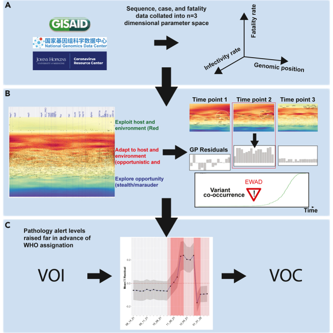
To address the impact of WGA of SARS-CoV-2 on host-pathogen balance driving the spatial-temporal dynamics of spread and pathology, we applied GP to generate allele-based phenotype landscapes that describe on a nucleotide-by-nucleotide basis the SCV relationships linking viral spread to pathology across the entire ∼30,000-bp SARS-CoV-2 genome (Figure 1). Figures 1A–1C shows the process for generating the SCV relationships. These SCV relationships are defined by three axes that include (1) allele genome position (x axis)), (2) allele frequency-weighted infectivity rate ($\overline{IR})$ (spread) (y axis), and (3) allele frequency-weighted fatality pathology rate ($\overline{FR}$) (z axis, color) (Figure 1A). These three features, when generated in the context of time, allow us to quantitatively image the spatial-temporal features contributing to spread and pathology through the different phases of the pandemic as a covariant collective of the designated VOCs in the universal context of the global mutation load (see methods for full details), visualized in daily SCV landscapes (Figures 1D and 1E, with zoomed inset).

Figure 1.

Illustration of the GP regression approach

(A) Data ingestion and pre-processing. Genotypic data from SARS-CoV-2 isolates and phenotypic data (cases and deaths) are gathered daily from NGDC and JH resource, respectively. For each reported SARS-CoV-2 mutation, allele frequency-weighted $\overline{\mathit{I}\mathit{R}}$ and $\overline{\mathit{F}\mathit{R}}$ are computed.

(B) SARS-CoV-2 mutations (alleles) are positioned by their genomic positions (x axis) and $\overline{\mathit{I}\mathit{R}}$ (y axis) and colored by $\overline{\mathit{F}\mathit{R}}$ (z axis). The pairwise spatial relationships (indicated by black lines) are analyzed by GP regression. Shown is a simplified plot showing only 50 mutations for clarity.

(C) As a first step in GP regression modeling, a variogram is computed (an illustrative example is depicted) showing spatial relationships between the separation distance of paired data points in (B) (x axis) and the spatial variance of $\overline{\mathit{F}\mathit{R}}$ relative to $\overline{\mathit{I}\mathit{R}}$ (y axis).

(D and E) GP regression maps of genomic position (x axis), and log-transformed $\overline{\mathit{I}\mathit{R}}$ (y axis) and $\overline{\mathit{F}\mathit{R}}$ (color scale, z axis) for SARS-CoV-2 genome (data in this example are for 9/15/20). $\overline{\mathit{F}\mathit{R}}$ is predicted across the whole landscape according to the variogram computed in (C), where output is an average of surrounding sample points, weighted by a function of distance given by the variogram.

(D) Black dots represent variant input values used to compute GP regression, with dot sizes proportional to the allele frequency of the mutations. Vertical dotted blue lines are boundaries between SARS-CoV-2 proteins, annotated on the top axis.

(E) Input variants are shaded light gray for clarity of VOCs. Contour lines are drawn at 10% and 25% percentiles of global variance estimated for model predictions (C). Labels on the map are signature mutations for Alpha (black), Beta (blue), Gamma (green), and Delta (brown). The zoomed inset shows the region with most VOC mutations in more detail, with all input mutations and contours that are used to train the GP regression model.

The expanding time frame of SCV relationships

Focusing on the first stages of the pandemic up through to the time of the Delta VOC, we show six tri-monthly snapshots from the time lapses, each taken mid-month and annotated for the set of signature Alpha VOC (Figure 2A, panels 1–6, analysis of distance and variance in Figure 2B) and the Delta VOC (Figure 3A, panels 1–6, analysis of distance and variance in Figure 3B). See supplemental information for Beta and Gamma VOCs (Figures S2 and S3) and Video S1. Movie of allele phenotype landscapes across the pandemic timeline for VOCs Alpha, Beta, Gamma, DeltaImages are annotated with four VOC signature mutations (Alpha, black; Beta, blue; Gamma, green; Delta, Brown). Details as in Figures 2 and 3, Video S2. Movie of allele phenotype landscapes across the pandemic timeline for Alpha VOC. Images are annotated with VOC signature mutations. Details as in Figures 2 and 3, Video S3. Movie of allele phenotype landscapes across the pandemic timeline for Beta VOC. Images are annotated with VOC signature mutations. Details as in Figures 2 and 3, Video S4. Movie of allele phenotype landscapes across the pandemic timeline for Gamma VOC. Images are annotated with VOC signature mutations. Details as in Figures 2 and 3, Video S5. Movie of allele phenotype landscapes across the pandemic timeline for Delta VOC. Images are annotated with VOC signature mutations. Details as in Figures 2 and 3 for the full time lapses for each VOC. Beginning with 5/15/20 for the Alpha VOC (Figure 2A, panel 1), only a few mutations are reported including a mutation in nsp3 (T1001I), four in Spike (21991del, 21765del, P681H, T716I), and two mutations in the nucleocapsid (NC) gene (R52I, S235F), both in areas of relatively high $\overline{FR}$ (Figure 2A, orange to red). The next time point 3 months later (Figure 2A, panel 2) reveals the emergence of an important Spike mutation (501N- > Y) at the bottom of the map with very low $\overline{IR}$/$\overline{FR}$, while the rest of the defining mutations for Alpha VOC are already migrating to higher $\overline{FR}$ areas. By 11/15/20 (Figure 2A, panel 3), all assigned mutations for Alpha VOC are present, and all in relatively high $\overline{FR}$ regions reflecting their initial impact on pathology as a potential opportunist in a naive host environment, particularly the aging population. From this time point onward, the distribution of mutations on the map increasingly “compacts” where the relative GP defined SCV relationships between mutations get smaller, both at the 5′ and 3′ ends of the SARS-CoV-2 genome (Figure 2A, panels 7 and 8). These VOC-containing clusters, as a covariant collective, migrate toward the top of the allele phenotype landscape with higher $\overline{IR}$ suggestive of cooperation in WGA features impacting both spread and fatality (Figure 2A, panels 4–6). However, their collective migration occurs in the context of the increasing number of variant dark matter variants that retune the GP-based allele phenotype landscape features over time (Figure 2A, black dots). These hidden supporting residues found in the global population contribute to the observed lineage diversification from our GP-based SCV global perspective.

Figure 2.

Time lapse of viral genome allele phenotype landscapes

(A) Alpha VOC showing six tri-monthly time points between May 2020 and August 2021. $\overline{\mathit{I}\mathit{R}}$ (y axis) and $\overline{\mathit{F}\mathit{R}}$ (z axis) are log-transformed, genomic position is scaled to a (0–1) scaled from 5′ to 3′ of the RNA sequence encompassing ∼30,000 bp with 5′-end located at the origin of the x axis. Vertical dotted blue lines are boundaries between SARS-CoV-2 proteins, annotated on the top of each figure. Input variants are in shaded color, with dot sizes proportional to allele frequency of the mutations. Contour lines are drawn at 10% and 25% percentile of global variance estimated for model predictions (Figure 1C).

(B and C) (Left) Average distance between Alpha VOC signature mutations defined by x axis (genomic position) and y axis coordinates ($\overline{\mathit{I}\mathit{R}}$) as described in Figure 1B for each of the six time points shown in (A). The gray ribbon marks the 95% confidence interval. (Right) Average spatial variance of $\overline{\mathit{F}\mathit{R}}$ (z axis) between Alpha signature mutations defined by x axis ‘Genome position’ and y axis coordinates ($\overline{\mathit{I}\mathit{R}}$) as described in Figure 1B for each of the six time points shown in (C). The gray ribbon marks the 95% confidence interval.

Figure 3.

Time lapse of viral genome allele phenotype landscapes

(A) Delta VOC showing six tri-monthly time points between May 2020 and August 2021. $\overline{\mathit{I}\mathit{R}}$ (y axis) and $\overline{\mathit{F}\mathit{R}}$ (z axis) are log-transformed, genomic position is scaled to a (0–1) scaled from 5′ to 3′ of the RNA sequence encompassing ∼30,000 bp with 5′-end located at the origin of the x axis. Vertical dotted blue lines are boundaries between SARS-CoV-2 proteins, annotated on the top of each figure. Input variants are in shaded color, with dot sizes proportional to allele frequency of the mutations. Contour lines are drawn at 10% and 25% percentile of global variance estimated for model predictions (Figure 1C).

(B) (Left) Average distance between Delta VOC signature mutations defined by x axis (genomic position) and y axis coordinates ($\overline{\mathit{I}\mathit{R}}$) as described in Figure 1B for each of the six time points shown in (A). The gray ribbon marks the 95% confidence interval. (Right) Average spatial variance of $\overline{\mathit{F}\mathit{R}}$ (z axis) between Delta signature mutations defined by x axis ‘Genome position’ and y axis coordinates ($\overline{\mathit{I}\mathit{R}}$) as described in Figure 1B for each of the six time points shown in (A). The gray ribbon marks the 95% confidence interval.

The primary factor responsible for the observed SCV compaction is the increase in the number of Alpha VOC detections in response to population testing leading to higher allele frequency weights in $\overline{IR}$; however, we still detect significant changes in the SCV relationships of all VOC mutations in response to the changing local environments revealed by predicted $\overline{FR}$ (Figure 2A, panels 1–6, z axis). Intriguingly, by 2-15-21 (Figure 2A, panel 4), we already notice that the mutations in the 3′ region of the SARS-CoV-2 genome have migrated to a low $\overline{FR}$ region and this becomes more evident in successive snapshots, where all Alpha mutations lay in a high $\overline{IR}$/low $\overline{FR}$ region at the top of the allele phenotype landscape. This trend likely reflects the beginning of the impact of host countermeasures, including innate and adaptive immune responses, vaccine availability, and physical interventional measures such as masks and social distancing, clearly illustrating the impact on fatality but less so on the global spread of variants seen in the continued increase of $\overline{IR}$ at this time frame (Figure 2A, panels 4–6).

For Delta VOC, the early time point (Figure 3A, panel 1 [(5/15/20]) has two NC mutations already in high $\overline{FR}$ (203R- > M, 377D- > Y), similar to what was observed with Alpha (Figure 2A, panel 1). These mutations are in two of the three disordered domains of NC (LINK and CTD) where most protein-protein and protein-RNA interaction sites occur.⁵⁰ By 11/15/20 (Figure 3A, panel 3), almost all signature mutations for Delta VOC are in relatively high $\overline{FR}$ regions and this continues through the next time point (Figure 2B, panel 4: 2/15/21) where the mutations are now more spread over the $\overline{IR}$ axis than was observed in Alpha (compare Figure 2A, panel 4, with Figure 3A, panel 4). There are almost two orders of magnitude of difference in $\overline{IR}$ between 478T- > K (Spike) and 377D- > Y (NC) pointing to the fact that there is a wide difference in spread of signature mutations in Delta VOC reflecting different evolutionary trajectories promoting success. These results, along with the emergent variant dark matter, suggest that the Delta VOC is still evolving in the context of the worldwide population as a “predator,” whereas Alpha variants have comparable values at these time points, suggesting that a consolidation of WGA function has been achieved and curiously, appears to be the endpoint in its race for fitness through SCV relationships—reflecting the limitations of its GP evolved WGA.

In the last two snapshots (Figure 3A, panels 5 [(5/15/21] and 6 [(8/15/21]), the Delta VOCs are now located in a high $\overline{IR}$, low $\overline{FR}$ cluster, as seen for Alpha but at an even lower $\overline{FR}$/$\overline{IR}$. Counts for Delta VOC, as of May 2021, were at least 100 times lower than Alpha VOC (Figure S4), reflecting the lower cumulative spread of Delta compared with Alpha VOC at this point in time, although Delta’s subsequent surging prevalence in the pandemic dwarfed the real-time values of the Alpha VOC, suggestive of SCV-based optimization for spread. For Beta and Gamma VOCs, we observe more of a mixed behavior over time compared with the trajectories of Alpha VOC and Delta VOC with only few mutations (e.g., 501N- > Y) moving into high $\overline{IR}$, low $\overline{FR}$ clusters at later time points (Figures S2 and S3).

Combined, these results capture the striking VOC divergence in allele phenotype landscape features in the context of the global pandemic. They suggest that these VOCs are progressively channeled into unique collectives of SCV relationships in the context of an increasingly more combative host response environment, limiting their capacity to achieve further prominence on a worldwide scale.

Temporal co-occurrence patterns give a way of tracking VOC emergence

To provide an alternative approach to the patterns of emergence captured through GP analyses and to augment and validate our GP approach, we generated a comprehensive view of mutation co-occurrence across the entire arc of the SARS-CoV-2 pandemic. For each virus isolate, sequence alignment against the reference SARS-CoV-2 genome reports the mutations called on that particular sequence. Such alignments can be mined systematically for co-occurrence of mutations over time, where co-occurrence is simply the count of mutations occurring together on the same viral sequence (see methods). Co-occurrence analyses let us track evolvability, reflecting increasing mutational burden in genome variation events, events that likely contribute to lineage focus on spread and pathology.

To highlight co-occurrences driving emergence of VOCs Alpha, Beta, Gamma, and Delta, we first tracked cumulative co-occurrences among the defining mutations for every day starting 9/15/21 up to 8/22/21 and computed a daily average co-occurrence by averaging all cumulative co-occurrence values available daily for each of the VOCs. Average co-occurrence over time for the four VOCs is shown (Figure 4A, left panel; zoom of Beta/Gamma/Delta VOC timeline plots shown in the right panel). Differences between VOCs are further evident in the patterning of their representative co-occurrence matrices (Figure 4B). The first VOC to emerge, Alpha, has a uniform distribution of co-occurrences across the signature mutations of this viral strain, suggestive of an opportunistic break in its evolving host-pathogen encounters. This is not the case for later emergent VOCs. See supplementary results for more details.

Figure 4.

Co-occurrence over time for VOCs

(A) Timeline plots showing average cumulative co-occurrence (co-occurrence) over time for the four VOCs on the same scale (left), and zoom view on the later VOCs (Beta, Gamma, Delta).

(B) Representative co-occurrence matrices showing co-occurrence counts between the signature mutations of each VOC. For both (A) and (B): Alpha VOC, black; Beta VOC, blue; Gamma VOC, green; Delta VOC, brown.

To track the actual number of co-occurrences between signature mutations of a VOC versus all possible co-occurrences at a specific time point, we defined VOC co-occurrence density as the ratio between the number of non-zero co-occurrences in the VOC co-occurrence matrix (Figure 5, lower panels in each VOC) over the total number of possible co-occurrences. Here, an empty VOC co-occurrence matrix has a density of 0, and one with no zeroes has a density of 1. As an example, we computed co-occurrence density for each of the four VOCs between September 2020 and August 2021 (Figure 5, lower panel for each VOC). Analysis of co-occurrence density curves for each VOC over time reveals that for the two early-onset VOCs (Alpha and Beta), the VOC co-occurrence density has an “all or none” behavior—going from near zero to one in a single day (Figure 5, lower panels for Alpha and Beta VOC). This event is many weeks ahead of the time where VOC average co-occurrences enter a fast growth phase (Figure 5, upper panels Alpha and Beta, green curves).

Figure 5.

For each VOC (Alpha, Beta, Gamma, Delta), the upper panel reports min co-occurrence, max co-occurrence, average co-occurrence, and range (max co-occurrence minus min co-occurrence) between 9/15 and 8/22

The lower panel shows co-occurrence density, which is the number of non-zero co-occurrences over all possible co-occurrences, standardized for the range of 0–1, for the same time interval. To characterize more precisely co-occurrence patterns emerging for the four VOCs, we tracked max co-occurrence, min co-occurrence, and co-occurrence range over time instead of solely the average co-occurrence described above (upper panel of each). For Beta and Gamma, we observe a “high range” pattern where the difference between max and min co-occurrence (range co-occurrence: red line) increases over time and is above the curve for average co-occurrence (green line). Conversely, Alpha and Delta VOCs show a low range (red line) that is consistently below the average co-occurrence curve (green line) after co-occurrences begin accumulating at a steady pace. Beta and Gamma lineages are thought to boost the immune escape capabilities of the virus, while Alpha and Delta variants are more efficient in enhancing infectivity and spread. Thus, based on the detailed co-occurrence profiles, we can discriminate between different functional classes of VOCs.

In contrast, for the later VOCs (Gamma and Delta), co-occurrence densities exhibit an exploratory behavior where in the early phase few co-occurrence options are explored for a longer time interval before the jump to the full spectrum of co-occurrences, reflecting its predatory behavior. Here, the time at which the jump is observed is nearly proximal to the beginning of the sustained growth phase where the increasing slope of the co-occurrence average curve starts (Figure 4A, e.g., green curve, Gamma). This contrasts with the “all or none” VOC co-occurrence densities for Alpha and Beta (Figure 5, lower Gamma and Delta panels). An intermediate level of acquisition of co-occurrence is particularly evident within the Delta VOC capturing co-occurrence links for months up to 0.4–0.5 (40%–50%) of co-occurrence discovered prior to the jump to the full co-occurrence set. To track the spread and pathology of each VOC in the context of evolving host responses, we performed a joint analysis of all VOCs by tracking their signature mutations through their genomic co-occurrences to provide detailed insight into the convergence of co-occurrence for each possible co-occurrence seen in the pandemic (Figure S5). These results suggest that the virus WGA is evolving improved search strategies over time across a seemingly intractable number of mutation-sensitive co-occurrences influenced by the supporting variant dark matter. Thus, evolving VOC co-occurrence relationships highlight potential pathogen fitness strategies that likely contribute to evolutionary success or failure. These potential strategies are missing from existing perspectives of viral spread and pathology.

GP residuals provide a clear early warning of VOC emergence

Because the co-occurrence analysis alone is not linked to the real-world infection and fatality features, it is not enough to inform whether a certain combination of mutations will eventually result in a VOC that challenges the evolved/evolving host responses that, as a covariant collective, ultimately dictates virus spread.

To track the spread and pathology of each VOC in the context of evolving host responses, we performed a joint analysis of all VOCs by tracking their signature mutations through their genomic co-occurrences (Figure S5) over time in conjunction with GP-based $\overline{IR}$ and $\overline{FR}$ SCV relationships (Figures 2 and 3). Specifically, we examined whether allele phenotype landscapes could be used as an EWAD⁵¹ system for the emergence of VOCs reflected in GP principled relationships dictating global spread and pathology. An EWAD system for spread and pathology is looking for a signal that ideally changes significantly during the early phase of the transition, reaches a maximum, and then quenches when the phenomenon enters a steady state, reflecting accomplishment of the optimized goal across the population, often leading to its diminution in the host population due to the Red Queen effect.⁵²

To assess the potential of an emergent EWAD signal as the SARS-CoV-2 evolves in response to host countermeasures, we focused on “$\overline{FR}$ residuals.” In GP modeling at a given time point in the pandemic (Figure 6A, x axis), $\overline{FR}$ residuals are defined as the difference between the observed and predicted $\overline{FR}$ values (Figure 6A, y axis, observed $\overline{FR}$ minus predicted $\overline{FR}$). The observed $\overline{FR}$ for a mutation is the explicit assigned $\overline{FR}$ of that mutation used for the input data in GP that does not incorporate the impact of other mutations, while the predicted $\overline{FR}$ for the mutation generated by GP is a proximity weighted average of the observed $\overline{FR}$ value in the context of its surrounding mutations in the phenotype landscape that includes the hidden relationships driven by the variant dark matter. If the observed $\overline{FR}$ is lower than the predicted $\overline{FR}$ for a mutation (i.e., a negative GP residual value [Figure 6A, left panel]), it indicates that the $\overline{FR}$ for the mutation is lower than the $\overline{FR}$ of surrounding mutations in the phenotype landscape, therefore underperforming relative to the surrounding VOC/variant dark matter in terms of $\overline{FR}$. In contrast, if the observed $\overline{FR}$ is higher than the predicted $\overline{FR}$ for a mutation (i.e., a positive GP residual value [Figure 6A, left panel]), it indicates that this mutation has a higher $\overline{FR}$ than its surrounding mutations—therefore overperforming in its pathology as defined by $\overline{FR}$ relative to the surrounding VOC/variant dark matter. Overperformance is consistent with the interpretation that is emerging as a prominent player in disease pathology as measured by $\overline{FR}$. These relationships we take as our definitions of under- or overperformance, reflecting how a variant’s actual pathology ($\overline{FR}$) compares with its GP-based pathology as predicted by the surrounding variant dark matter. In addition, the mean $\overline{FR}$ residual’s location above/below the baseline can tell us something about the nature of the impending cluster of variants reflecting their potential impact on pandemic progression. Therefore, the GP-based $\overline{FR}$ residual value represents a real-time monitor of the collective behavior of the global virus system versus the actual sparse measurements defined by a VOC mutation designated at the 75% frequency level used by the epidemiological community to track strain importance.

Figure 6.

EWAD analysis of Alpha, Beta, Gamma, and Delta VOCs

(A) Graphical explanation of GP regression residuals. GP predictions are covariance-matrix weighted averages of the observed values, so a GP regression prediction is a point comprising the proximity weighted information of its surrounding observed values in the variant dark matter. The GP residual, calculated by using observed value minus the predicted value reports the difference between the mean observed $\overline{FR}$ of that variant and the predicted $\overline{FR}$—the weighted average of its surrounding variants. As illustrated, a positive GP residual indicates that the observed mean $\overline{FR}$ of that variant is higher than the mean weighted averaging of the $\overline{FR}$ for surrounding variants, while a negative GP residual indicates the predicted mean $\overline{FR}$ of that variant is lower than the mean weighted averaging of the $\overline{FR}$ for surrounding variants. GP residual values represent a real-time monitor for the differences of predicted variant $\overline{FR}$ based on SCV analysis.

(B–I) For each VOC (B and C, Alpha; D and E, Beta; F and G, Gamma; H and I, Delta), we report its average co-occurrence (co-occurrence plots: B, D, F, and H) together with the mean $\overline{FR}$ residuals for its signature mutations (mean, blue line; 95% confidence interval, gray shade) computed weekly along the selected time interval (EWAD plots: C, E, G, and I). We examined the time interval between September 20 and May 21, and based on average co-occurrences, we selected six representative time points covering the flat, early, and sustained co-occurrence growth phases for each of the VOCs (see numbered points in graphs B–I). The baseline for EWAD is set to 0 ± 0.05 obtained by empirical randomization (dashed red line at 0 in EWAD plots) (C, E, G, and I) where for a VOC including n signature mutations, we computed the mean $\overline{FR}$ residuals of thousands of random sets of n mutations yielding the interval near zero the random (null) EWAD signal. We then defined two alert levels, pathology alert level 1 (PAL1) (light red shades: C, E, G, and I) and pathology alert level 2 (PAL2) (dark red shades: C, E, G, and I) based on a heuristic that takes into account the degree of change over time, the magnitude of change, and the persistence over time where PAL1 includes two consecutive points whose combined change in mean $\overline{FR}$ residual is above 0.05, and/or where both mean $\overline{FR}$ residual and its 95% confidence interval are above/below zero. PAL2 includes three consecutive points whose combined change in mean $\overline{FR}$ residual is above 0.1. Stars show the date that each variant was designated a VOC by the WHO.

EWAD residuals reveal striking real-time signals of pathology, codified in pathology alert levels

By using as input the defining mutations of the Alpha, Beta, Gamma, and Delta VOCs as our sparse collection of measured values for GP-based analyses, we reasoned that the calculated mean of $\overline{FR}$ residuals, where the mean is the averaged value of the $\overline{FR}$ residuals for a given time frame (see methods), could be used as output across the entire pandemic time line to detect potential features in advance reflecting the emergence of VOC from the variant dark matter. Because mean $\overline{FR}$ residuals highlight coordinated changes in real time in the observed $\overline{FR}$ versus the predicted $\overline{FR}$ based on the SCV relationships within the evolving variant dark matter, they provide an EWAD for emerging VOCs.

We first examined the mean $\overline{FR}$ residuals for all the mutations defining Alpha, Beta, Gamma, and Delta VOCs at weekly time points, and plotted the mean $\overline{FR}$ residual value for each VOC as a measure of their changing GP-based relationships to define globally the emergent evolution of SARS-CoV-2 lineages. Initial efforts focused on the average co-occurrence cumulative counts over the time interval between September 2020 and May 2021. We selected six representative time points covering the flat, early, and sustained growth phases for each of the VOCs Alpha, Beta, Gamma, and Delta VOCs for co-occurrence (Figures 6B, 6D, 6F, and 6H) and their mean $\overline{FR}$ residuals (Figures 6C, 6E, 6G, and 6I, blue line) for analyses. We first assign a zero baseline that is set to 0 ± 0.05 by empirical randomization where any overlap of the mean $\overline{FR}$ residuals with the baseline reflects the high probability that the calculated mean relationships are unrelated to the emergent VOC under consideration (Figures 6C, 6E, 6G, and 6I, red dashed line).

To assess potential EWAD signals, we defined two pathology alert levels (PAL): PAL1 (Figures 6C, 6D, 6G, and 6I; light red shade) and PAL2 (Figures 6C, 6D, 6G, and 6I; dark red shade), which considers the degree of change over time, the magnitude of change, and the persistence over time—detailed as follows. PAL1 is defined either as (1) two consecutive points (Figure 6B, x axis) whose combined change in mean $\overline{FR}$ residuals (Figure 6B, y axis) is more than 0.05, and/or (2) both mean residual and its 95% confidence interval above or below the zero baseline. PAL2 is defined as three consecutive points whose combined change in mean $\overline{FR}$ residuals is above 0.1. Two empirical alert levels were chosen as they seemed a reasonable trade-off between an overly simplistic single-alert model, and the additional complexity of multiple alert levels (where PAL1 is an invite to watch closely, whereas PAL2 incites to possible action).⁵¹ These alert levels were chosen to show significant deviations from the basal state that could have more rigorous definitions, as our understanding of their root cause evolves in future work. We next examined EWAD development over time for Alpha and Omicron as examples at the extreme ends of the pandemic, with Beta, Gamma, and Delta explained in detail in the supplementary results.

To test the statistical significance of the EWAD PAL system, 15 mutations similar to the size of signature mutations for Alpha and Gamma VOC were randomly chosen and monitored over seven tri-weekly time points between 11/17/20 and 5/18/21. Whereas the mean $\overline{\mathrm{F}\mathrm{R}}$ residuals corresponding to VOC signature mutations show a coordinated, EWAD signal of potential use for variant surveillance (see the bar plots in Figures S6 and S7), residuals for these randomly chosen mutations show a rather random behavior over time, not correlated with specific temporal events. The full analysis was repeated with thousands of random sets of mutations whose set size is the same as the VOC signature mutations considered here (10–15 mutations) to determine if the EWAD results were statistically significant and unique to VOC, or if they were just a map-wide property that could be observed for any random set of mutations. Remarkably, a great majority of randomly selected mutations did not present any coordinated behavior at the level of $\overline{\mathrm{F}\mathrm{R}}$ residuals across the selected time window (empirical p values <10⁻³ for all VOCs), providing evidence that the observed EWAD patterns are specifically associated with distinctive VOC mutations. The mutation sets for Alpha, Beta, Gamma, and Delta VOCs were compared with five randomly selected sets of mutations from the data in order to validate the significance of the differences between the VOC mutations and randomly chosen mutation sets. These results showed conclusive differences, as described in full in Figure S8. These results have important implications for the future prediction of unknown VOCs prior to their emergence by focusing on emerging variants in the variant dark matter comprising high spread with either low or high pathology.

An EWAD example: Predicting the Alpha VOC

Alpha VOC was first detected in November 2020 from a sample collected in the United Kingdom in September 2020⁵³ and declared a VOC on 12/15/20 (Figures 6B and 6C; star). Although our co-occurrence data track down precisely this first Alpha isolate as seen in the co-occurrence density plot for Alpha (Figure 5, transition to full co-occurrence density on 9/16/20 due to a single isolate), co-occurrence data alone at that time point does not reveal that this event would turn into a widespread VOC, as we have few detections and almost no growth indicated by the flat average co-occurrence (Figure 6B; time point #1, 10/15/20). Strikingly, we note on the EWAD plot (Figure 6C) that this point is already marked as PAL1, being significantly below the baseline but with a broad confidence interval, which was activated just 2 weeks after the discovery of the first isolate. Being below the baseline suggests that the mean $\overline{FR}$ residual for the Alpha VOC is below what we might otherwise expect, consistent with an EWAD signal of PAL1. By underperforming relative to surrounding variant dark matter, this suggests the emergent cluster is hidden from view, having a lower fatality rate than expected, but by triggering PAL1 it reveals itself as a potential VOC (Figure 6C).

On 11/14/20 (Figure 6B, time point #2), we see a change in the growth regime, with a rapidly increasing slope transitioning from flat to consistent growth while the number of worldwide detections remains low (Figure 6B, ∼200). The EWAD plot (Figure 6C) reveals a remarkable change with a steep decrease in mean $\overline{FR}$ residuals exceeding 0.1 and a more compact confidence interval resulting in PAL2 activation beginning on 10/16/20. Looking at the individual $\overline{FR}$ residuals in the allele phenotype landscape (Figure S6), we see that the change is driven by mutations on the map that are compacting in both the 5′ and 3′ regions where the average distances of Alpha VOC mutations decrease between 8/15/20 and 2/15/21 (Figure 3A). The mean $\overline{FR}$ residuals consistently fall to more negative values, suggesting that the Alpha VOC is seeking to optimize covariance relationships between these underperforming driver mutations relative to the supporting passenger variant dark matter. Hence, even with a very low number of detections, the mean $\overline{FR}$ residuals appear to respond quite sensitively to changes in the entire growth regime in a coordinated fashion across the worldwide population. The change would appear negligible and overlooked if examined at the level of hierarchical clustering (mutation counts) or co-occurrences alone, whereas the stark, coordinated change seen within mean $\overline{FR}$ residuals based on GP modeling induces a solid early warning for this set of variants.

The 11/20/21 time point (Figure 6B, time point #3) captures the increasing co-occurrence growth rate with ∼800 more detections within 8 days, further showing a coordinated decrease in the mean $\overline{FR}$ residuals (Figure 6C) and accompanied by compaction of mutations on the allele phenotype landscape in the 5′ cluster (Figure 3A). The EWAD signal (Figure 6C) keeps increasing steadily and stays in PAL2, confirming the trend of a strong early warning signal revealed at the previous time point. Again, at this early stage of spread for Alpha VOC, counts alone could be easily overlooked; in contrast, monitoring of mean $\overline{FR}$ residuals provides a clear EWAD signal many weeks ahead of the official (and after-the-fact) designation of these mutations as a VOC.

After an additional 1.5 months (Figure 6B, time point #4, 1/12/21), when the co-occurrence is entering a steady, quasi-exponential growth phase (with over 50,000 viral genomes sequenced bearing the Alpha co-occurrence signature), the average distance between mutations in the 5′ cluster is smaller and at higher values of $\overline{IR}$ in the map corresponding to lower $\overline{FR}$ (Figure S6; panel 4). The mean $\overline{FR}$ residuals exhibit the same consistent pattern of negative values as the previous time point but are more uniform and at a lower magnitude (Figures 7C and S6, panel 4, bar plot). On the EWAD plot (Figure 7C, blue line), mean $\overline{FR}$ residuals are steadily increasing with confidence interval compaction, reflecting improving accuracy of the prediction by GP, still in PAL2. Hence, the collective signal defined by the mean $\overline{FR}$ residuals begin attenuating after reaching the maxima observed in the EWAD phase given its sensitivity to (1) growth rate change and (2) the fact that detections are now in a steady growth regime reflecting balance with supporting variant dark matter in the absence of new competition.

Figure 7.

Omicron VOC co-occurrence and EWAD spanning 8/15/21 to 3/20/22

(A) Time line plot showing average cumulative co-occurrence over time for combined Alpha, Beta, Gamma, and Omicron VOC defining mutations (Delta is out of range with values near 1M and is therefore omitted).

(B) EWAD plot for combined Omicron where mean $\overline{FR}$ residuals (blue line with 95% confidence interval, gray shade) for Omicron signature mutations computed weekly along the selected time intervals. The baseline for EWAD is set to 0 ± 0.05 by empirical randomization (dashed red line at 0; details as in Figure 6). Alert levels defined as in Figure 6.

(C) Time line plot showing average cumulative co-occurrence over time for Omicron 1.1.529 and sub-lineages BA.1 and BA.2 for defining mutations.

(D and E) Omicron sub-lineages BA.1 and BA.2 sub-lineages with co-occurrence over time and EWAD analysis between 1/17/22 and 3/20/22. EWAD plots for BA.1 and E. BA.2 where mean of $\overline{FR}$ residuals (blue line; 95% confidence interval, gray shade) signature mutations computed weekly along the selected time interval. The baseline for EWAD is set to 0 ± 0.05 by empirical randomization (dashed red line at 0; details as in Figure 6). PAL defined as in Figure 6.

Finally, for the time points #5 and #6 (Figure 6B, sampled on 2/16/21 and 4/5/21, respectively) during the steady growth phase, mean $\overline{FR}$ residuals show no further compaction of the defining Alpha VOC (Figure S6; panels 5 and 6, allele phenotype landscape and bar plots), but rather a collective migration to a higher $\overline{IR}$ and lower $\overline{FR}$ region in both 3′ and 5′ clusters (Figure 6C, blue line; Figure S6, panels 5 and 6, allele phenotype landscape). The mean $\overline{FR}$ residuals modestly increase their magnitude while keeping their uniform, sign pattern (Figure S6; panels 5 and 6, bar plots), thus confirming the attenuated signal configuration initially observed at the previous time point. On the EWAD plot (Figure 6C, blue line), this translates to an approximately flat progression with a narrow 95% confidence interval still in PAL1 since both are well below the baseline. These results suggest a still underperforming variant that could reflect an underestimate of the pathology at this time point, although these results also suggest that Alpha has reached a steady-state equilibrium with the existing supporting variant dark matter and a more effective host environment response to its restricted covariant cluster of mutations.

While we focused on Alpha VOC, EWAD plots can be described that illustrate that different GP-based tactical strategies seen for Beta, Gamma, and Delta VOCs (Figures 6D–6I, see supplemental results). Interestingly, for Beta VOC, the VOC call was made well before PAL1 (Figure 6E) suggesting it was premature, consistent with the fact from a global perspective it remained highly regionalized and fizzled out quickly (outbreak.info/²⁵), questioning the utility of the 75% VOC designation as a reliable tool for designating a VOC in the absence of appreciation of the global covariance dictating host-pathogen balance.

Thus, mean $\overline{FR}$ residuals extracted from allele phenotype landscapes have many desirable traits of an EWAD system. The results are statistically significant and unique to each of the VOCs. Importantly, they are not just map-wide properties that could be observed for any random set of mutations, given that if we repeat the analysis with thousands of random sets of mutations whose set size is the same as the Alpha, Beta, Gamma, and Delta VOCs, the majority of the randomly selected mutations will not present any coordinated behavior at the level of mean $\overline{FR}$ residuals across the selected time window (Figures S9 and S10; empirical p value <10⁻⁴). Consistent with this view, we performed ablation studies for the four VOCs—where the signature mutations of each VOC were removed from the training set prior to GP regression and EWAD analysis. Importantly, for all four ablated sets, we discovered no significant differences between the ablated and the original models in terms of EWAD signal (Figure S11), thus highlighting the robustness of an early warning system with respect to the presence of specific sets of mutations.

These results provide strong evidence that the observed patterns are generated systematically in response to GP-based selection and unknown fitness rules enabling the emergence of a VOC in the context of the large variant dark matter background, providing evidence that the observed EWAD patterns are specifically associated with distinctive VOC mutations. The results have important implications for the future prediction of unknown VOCs prior to their emergence by focusing on emerging variants in the variant dark matter comprising high spread with either low or high pathology (Figures S9 and 10). Can this EWAD behavior also be observed with VOCs emergent at the latest stage of the spread and pathology?

A second EWAD example: Predicting the Omicron VOC

To capture the most recent phase of spread and pathology, we updated the GP map from 8/15/20 to 3/20/22 to include emergence of Omicron variants with the peak in cases in January 2021 almost entirely driven by BA.1 and its sub-lineage BA.1.1 where the VOC call was made on 11/26/21 (Figure 7A, star). Here, the Omicron VOC refers to the mutations common to all Omicron lineages found during this time frame^22,24,25 (Figure 7A). When tracking the co-occurrence density for Omicron defining mutations (Figure 7B), we detect a jump in Omicron VOC defining mutations at 10/23/20 (Figure 7B, time point #1) consistent with its robust surge across the worldwide population. An EWAD plot of mean $\overline{FR}$ residuals (Figure 7C, blue line, 95% confidence interval, gray shade) at this time point detects emergence and a rapid transition from PAL1 to PAL2 with the mean $\overline{FR}$ residuals at 10/23/22 to 11/01/22 going above the zero baseline—well before its emergence as a dominant strain in 12/23/22 to 1/20/21 (Figure 7B, time point #2). Not only do we have exceptionally strong EWAD signal, but a rise above the baseline suggests that the observed VOC $\overline{FR}$ data is overperforming the prediction—that is, the observed VOC $\overline{FR}$ data are above what we might otherwise expect in response to the surrounding variant dark matter. These results suggest that $\overline{FR}$ is now being challenged by evolving host responses reflecting the Omicron’s “marauder” mode in the face of increasing competition from the host. However, this changes rapidly with the emergence of BA.1 and BA.1.1.1, with a rapid drop in $\overline{FR}$ residuals indicating a rapid evolution to fitness that allows it to dominate the pandemic landscape in the context of the supporting variant dark matter background. A similar sensitivity in early stages of Omicron diffusion is observed on the allele phenotype landscape (Figure S12), full details in the supplementary text.

To gain insight into the evolution of just the emergent Omicron sub-lineages BA.1-BA.2, we added an additional 1.6 M viral sequences between 1/17/22 and 3/20/22 (for a total of over 5.4 M sequences processed) where spread remained a prominent feature in the evolution of SARS-CoV-2 Omicron strains relative to fatality—likely reflecting gains in host immune response and more effective clinical/social management of virus pathology (Figures 7D and 7E).^54,55,56,57 The BA.1 sub-lineage, identified on 11/15/21 and becoming dominant worldwide by 1/17/22, was the first VOC suggested to be able to completely escape from neutralizing antibodies induced by vaccination,⁵⁷ in essence resetting the host immune response balance. Subsequently, the BA.2 sub-lineage sharply increased heading into February and March of 2022.^55,56 As of March 2022, Omicron BA.2 was the dominant sub-lineage in most countries. BA.1 and BA.2 have many mutations in common (both being sub-lineages of the original Omicron B.1.1.529) but with 21 mutations in the Spike protein, differentiating the two sub-lineages.

We focused on sets of characteristic signature mutations for BA.1 and BA.2 (43 and 49, respectively) that are non-synonymous substitutions or deletions in their encoded viral proteins that occur in >75% of sequences within the overall Omicron lineage²² (Figure 7C). Once again, co-occurrence counts alone offer limited information regarding the progression and potential risk of the new sub-lineages. We performed separate EWAD analyses for Omicron sub-lineages BA.1 and BA.2 weekly between 1/17/22 and 3/20/22 (Figures 7D and 7E; blue lines, 95% confidence interval [gray shade]) for signature mutations. During this interval, BA.1 and BA.2 sub-lineages already have higher cumulative co-occurrence counts (Figure 7C) compared with the variants common to all Omicron (Figures 7A and 7B), with an accumulation rate increasing with BA.2>BA.1>Omicron. Interestingly, mean $\overline{FR}$ residuals for each of the BA.1 and BA.2 sub-lineages show similar EWAD signals at the early stages of the evolution, but then differentiate suggesting different evolutionary paths are evoked by the change in mutation load in the evolving BA.2. For BA.1, new activity between 1/24/22 and 1/31/22 induces another brief PAL1 (Figure 7D), but then the signal subsides to no-alert with a broad mean $\overline{FR}$ residuals for the following weeks (up to 3/20/22) above the baseline. The mean of the observed values are overperforming our prediction—that is, the predicted VOC fatality rate is above what we might expect, suggesting that the host is gaining the upper hand in mitigating impact, a conjecture supported by the fact that BA.1 counts reach a plateau (Figure 7C, blue line), marking the time point where it begins to lose influence in response to the rising dominance of BA.2 (Figure 7C, orange line). Intriguingly, BA.2 EWAD (Figure 7E) is already in PAL1 during the first week (1/17–1/24) and rapidly escalates to PAL2. These results indicate that the observed data are overperforming our prediction and that the predicted VOC fatality rate is above what we might otherwise expect based on the surrounding variant dark matter, reflecting a stealth/marauder search mode.⁵⁸ This rise above baseline quickly drops back to below the baseline, indicating that the observed data are now underperforming our prediction and that the predicted VOC fatality rate is below what we would expect based on surrounding variant dark matter, suggesting a change in response by the host population that challenges fatality. Remarkably, the alerts for BA.2 are triggered in mid-January, again weeks before more official warnings such as the official World Health Organization (WHO) VOC designation in late February.

The overall EWAD pattern for BA.2 (Figure 7D) strikingly resembles the one seen for the originating collection of Omicron variants (Figure 7B). This indicates that EWAD has value not only for newly emerging lineages represented by the strikingly different VOCs, but also for tracking the subsequent evolution of VOC sub-lineages, a current concern of health agencies.^59,60 These results suggest that the integration of genotypic and phenotypic data through GP-based residual analysis provides a temporal and sensitive EWAD output for pandemic performance to anticipate its trajectory across the worldwide population.

Discussion

We have introduced a system-based GP spatial covariance platform^32,33,34,38 (Figure 8) to plot the role of natural selection and global population fitness in driving host-pathogen relationships. Not only do we capture the distinctive patterns of evolution of each of the VOCs through $\overline{IR}$ and $\overline{FR}$ coordinates in allele phenotype landscapes, but we have shown that tracking these changes through GP reveals a hidden and largely uncharacterized agenda involving the supportive variant dark matter in pandemic progression. GP-based analyses suggest that successful allele changes found in emergent VOCs are using rules defined by covariant weighted proximity that evolves with time and that are predictable based on SCV relationships encompassing the entire collective. This is evidence of the potential for GP-based SCV to provide insights from a high-confidence natural selection view that are rooted in global biological variation.^32,33,34,38

Figure 8.

Flow diagram for modeling EWAD and performance using GP

Starting from the GP-based predicted allele phenotype landscape for each VOC (leftmost panel) in combination with the co-occurrences at different time points (second panel from left), GP residuals can be calculated to assign PAL1 and PAL2 danger alerts (third panel from left) predicting the host-pathogen responses weeks to months ahead of the official WHO VOC assignation. The performance characteristics in terms of impact on VOC pandemic features can be estimated by the position of the mean $\overline{FR}$ residuals below or above baseline (dotted line). Shown as an example is the result for Omicron emergence (Figure 7B).

It is now apparent that the “collective” strategy defined by our GP-based covariant predictions reveals the ability of the VOCs to differentiate themselves from one another and from the whole in response to the more slowly evolving host genome. These range from the “opportunistic” Alpha VOC trajectory to the “predatory” Delta VOC to the “stealth/marauder” modes of Omicron trajectories. For example, from Alpha VOC onward, the time spent searching for optimal covariant combinations to enhance viral spread increases because of emergent immunological host responses to pathogen aggression. Delta stands out as the first predator VOC, performing a successful extensive GP principled grid search by using a dominant 3′ SCV cluster—one that includes mutations in the Spike protein affecting resistance to immune surveillance, binding, and uptake—as well as the nucleocapsid (NC) protein involved in packaging the virus, contributing to viral load.^50,61 This compact SCV cluster is then extended by the stealth/marauder state of Omicron VOC involving specific mutations not only in Spike and NC, but to additional mutations in viral proteases and envelope proteins, indicating that successive surges may involve increasingly complex covariant search strategies using different viral components to increase spread and thus contribute to the changes in host pathology that may become better targets for therapeutic management. For example, newly emergent strains of Omicron, such as BQ.1, BQ.1.1, and BQ1.5, have gained significant ground with the Omicron subvariant Arcturus (XBB.16) now taking the lead. It is interesting to note that by tracking the differing search strategies, it is the Omicron’s “marauder” mode, in the face of increasing competition from the host, that has dominated and become the baseline from which subsequent sub-lineages are emerging, particularly in China as of June 2023. The spread of these sub-lineages, it has been argued, is largely driven by immune response evasion in the Spike protein.^62,63,64 However, this alone may not be the answer. Covariance across the entire genome is something that will need to be considered in future work by incorporating what is hidden from view (i.e., the emergent features of the variant dark matter such as Q556K in the ORF1a protein and Y264H in the ORF1b protein that are present in BQ.1 and BQ.1.1 but not BA.1 or BA.5). This can be done through the prism of GP-based SCV and EWAD to advance understanding of viral pathology and/or advancing new therapeutics,^63,65,66 as our GP analysis treats the virus as whole (the collective sum of its covariate parts) in driving the rapid evolution of the pandemic.

The EWAD system showcased here builds upon the SCV method we developed for inherited genetic disease.³² Instead of focusing on polypeptide sequence changes, it focuses GP-based modeling of allele changes for all ∼30,000 bp comprising the SARS-CoV-2 genome, which raises the possibility that in the future could be applied to both coding and non-coding sequences. In addition, it adds the use of co-occurrences and residuals to the analysis allowing for not only the identification of possible VOCs well in advance of their WHO assignation (as can be seen in Table 1), but also giving a covariant-based description of the qualitative/quantitative behavior of those emerging variants. For example, representative heatmaps showing the mutation co-occurrence matrices during the early, mid, and late stages of the pandemic can be seen in Figures S13–S21, and for Delta specifically in Figures S22 and S23. Thus, computational analysis, merging the insights from GP-based mean $\overline{FR}$ residuals with co-occurrence maps, can provide an EWAD framework, where the averaged residuals are the difference between predicted and observed values, to account for host fitness relative to the emergent pathogen aggression. EWAD provides the ability to forecast the emergence of a VOC through both the slope dynamics of the mean $\overline{FR}$ residuals and the spatial-temporal compaction of the cluster reflected in co-occurrence densities. As a novel application of the GP-based SCV approach, the mean $\overline{FR}$ residuals also provide a performance index relative to the EWAD baseline—indicating the status of the VOC collective in response to the evolving (and largely hidden from view) variant dark matter—the evolution of which, for example, can be seen for nsp12 (Figure S24).

Table 1.

Table of VOC assignation showing EWAD PAL raised well in advance

VOC	Date of VOC assignation	Date of first PAL1	Date of first PAL2
α	18 Dec 2020	23 Sep 2020	16 Oct 2020
β	18 Dec 2020	5 Jan 2021	27 Jan 2021
γ	11 Jan 2021	26 Oct 2020	12 Dec 2020
δ	11 May 2021	10 Sep 2020	7 Nov 2020
ο	26 Nov 2021	23 Oct 2021	30 Oct 2021

While other models have been proposed that attempt to predict the spread of specific SARS-CoV-2 mutations,^67,68 to the best of our knowledge they do not link spread to fatality, or attempt to give qualitative/quantitative information about the potential features of a particular variant. Thus, these features allow us to see in advance the emergence of mutational clusters that could contribute to both spread and/or pathology before the virus advances to clinically stamped VOC status (Figure 8)—a result that does not appear to be tied to the presence of specific sets of signature VOC mutations as the ablation studies confirmed. This illustrates the usefulness of framing the pandemic evolution in terms of SCV relationships defined by the evolving worldwide viral genome as a collective—a view that expands on more traditional approaches such as hierarchical clustering. As such, GP-based SCV analyses of global allele distributions may provide a new way to address the dynamics of spread and fatality in pandemics. For example, Omicron had a strong EWAD signal harboring VOCs a full month before the lineage officially designated a VOC. Here, the lack of compaction of residuals suggests that this lineage is well-tuned to continue to evolve within its strain to succeed in successive waves, as has been captured by GP-based SCV for its sub-lineages highlighted above.^59,60

Besides the small sets of mostly non-overlapping signature mutations for each VOC lineage, the larger sets of all mutations that comprise the variant dark matter required for the full GP analysis are not generally considered as part of a VOC assignation when defining impact. In contrast, by tracing EWAD potential in terms of performance in the GP residual plots, we learn about the dynamics of viral evolution impacting their trajectory in the worldwide population. Here, the under- or over-powered feature of the prediction can give us a sense of how a given VOC achieved its current position in the context of downstream global spread and pathology. These results suggest that tracking via GP designated “variants being monitored,” variants of interest (VOIs), or a larger group of cluster subsets we refer to as covariant clusters with co-evolving high y axis $\overline{IR}$ values linked with $\overline{FR}$, could provide a more quantitative tool to assess risk management of disease from both virus and host perspectives. In general, our GP analysis attests to the need to expand our understanding of the variant dark matter in viral disease to fully appreciate the impact of variation in achieving fitness in host-pathogen race for dominance,⁶⁹ particularly the countermoves of the host adaptive and innate immune responses and/or social/clinical/political practices contributing to spread and fatality, particularly of the virus-sensitive aged population (Figure 8). The recently discovered ability to detect emerging variants in sewage may provide a broad and more consistent covariant collective of population behavior in each locale that is amenable to GP-based EWAD analysis.⁷⁰

The method introduced here for VOC early warning and variant surveillance has several features that are worth noting. It is a purely computational method for variant surveillance, using data from publicly available repositories (viral sequences, infectivity, and fatality data updated daily). In its early stage, it applies a novel multimodal data fusion approach across time-resolved genotypic and phenotypic data to obtain the input composite variables for GP modeling. The ML workflow implemented in the method differs from standard supervised ML methods (i.e., classification/regression) since it uses supervised ML (in the form of GP regression) as an intermediate step to generate data instead of an endpoint for the prediction, sharing similarities with generative modeling. Importantly, GP regression acts as an amplifier for small but robust differences through weighted proximity occurring in the phenotypic data over time, that are then exploited for the purpose of VOC anomaly detection.

The limitations in our method lie currently in its reliance on already identified variants in the population to pioneer the SCV framework. It is currently computationally prohibitive to examine all combinations of mutations seen in the SARS-CoV-2 data for their potential to become a VOC, although emergent variants being monitored and VOIs, as indicated above, provide a focused starting point in evaluating variant dark matter. Given the universal applicability of SCV,^{32,33,34,35,36,37,38,48} capturing emergence from the total viral variant load may be possible in other settings, including for example, influenza and HIV, where current collections of variant genotypes and associated phenotypes could serve as a collective for GP-based landscape descriptions.^{32,33,34,35,36,37,38,48,71}

In terms of computational resources, pattern generation by the GP method is highly efficient. Only 10 compute nodes and a few hours were used to image SCV maps for 700+ days of the pandemic. On the other hand, computation of co-occurrences can, in principle, be challenging both in terms of time and memory as the number of known viral mutations grew near-exponentially over time given the massive tracking efforts (for example, see Omicron co-occurrences in Figures S25 and S26). However, adopting a few strategies (detailed in methods) such as sparse data structures, and a cutoff on very low allele frequencies, computation of co-occurrences can be completed in a reasonable time frame on a moderately sized compute resource (e.g., a few days on 20 compute nodes). Code and examples for both GP and co-occurrence calculations is available at the GitHub public repository: https://github.com/balchlab/VSPsnap or Zenodo archival https://doi.org/10.5281/zenodo.8000486. Over recent months, the data coverage and quality of SARS-CoV-2 (such as the mutation frequencies tracked by outbreak.info [Figure S27]) has waned for many reasons—technical, social, and political. As such, our approach will be more challenging to apply. However, the strength of the GP model lies in its versatility and broader applicability given its use of only a sparse collection of variants such has already been applied to multiple human rare diseases.^{21,34,35,36,37,48} These efforts provide a new paradigm for development of therapeutics impacting genome-encoded sequence-function-structure relationships⁷¹ that can now be applied to viral genomes.

There is a fundamental dichotomy between the pandemic efforts focused on the “microscopic” (genes, mutations, proteins, biochemical and biophysics of virus life cycle, host cell biology) and “macroscopic” (cases, masks, vaccination, hospitalizations, deaths, social behavior, healthcare policies, politics, etc.) issues. Unfortunately, the necessarily integrated rules dictating these diverse covariant relationships remain largely unknown and hidden from view in the simple hierarchical clustering maps used to currently describe spread and pathology progression and guide health policy.²² In contrast, our GP-based SCV method can integrate both the micro- and macro- at atomic resolution.^32,33,34,38 For example, the migration to low $\overline{FR}$ regions in Alpha, Delta, and Omicron VOC lineages found at the top of allele phenotype landscapes is strongly correlated with the beginning of vaccination policies across many countries (not shown), indicating improvement in host fitness responses. Moreover, because even a simple estimator extracted from the modeling of GP-based $\overline{FR}$ residuals displays an unanticipated coordinated pattern of future relationships, there might be a number of additional properties that can be extracted that are more actionable than those revealed by simple hierarchical clustering.

In more general terms, we posit that GP-based features could help to elucidate the role of WGA in the context of micro- and macro-complexity observed at the host-pathogen interface à la the Red Queen challenge. These relationships are hidden within the variant dark matter and ignored as a collective except as a means of tracking evolutionary trajectories.⁶⁹ In contrast, GP-based WGA offers a starting point to begin to understand the complexity of coupled genomic and proteomic architectures, and how evolution uses this coupling through covariance to shape biological function.^{32,33,34,35,36,37,38,48} As host-pathogen biology moves into a new, rapid phase of management where molecular analysis, designer vaccines, and novel therapeutics can address the immediate need to lower human fatality, particularly in the aging population,^{2,3,4,5,6,7,8,9,10,11,12,13,14} an understanding of GP-based SCV relationships could allow for a more rapid and expansive exploration of disease at the level of the individual.^32,33,34,38 GP-based SCV principled ML insights could provide a more generalized approach for understanding pathogen fitness relative to host response (or vice versa) for management of risk in the clinic, given the versatility of phenotype landscapes to quantitatively frame the emergent Red Queen challenge.⁷²

Experimental procedures

Resource availability

REAGENT or RESOURCE	SOURCE	IDENTIFIER
Deposited data
Additional Supplemental Items are available from Mendeley Data	https://doi.org/10.17632/69zm32zvmn.1
Software and algorithms
Original code	https://doi.org/10.5281/zenodo.8000486
Other
CNCB publicly available individual sequence data	ftp://download.big.ac.cn/GVM/Coronavirus/gff3
CNCB publicly available individual meta data	https://bigd.big.ac.cn/ncov/release_genome
Johns Hopkins publicly available data	https://github.com/CSSEGISandData/COVID-19

Lead contact

Further information and requests for resources and reagents should be directed to and will be fulfilled by the lead contact, William E. Balch (webalch@scripps.edu).

Materials availability

All data are available in the main text or the supplementary materials.

Method details

Data generation and description

SARS-CoV-2 genome mutations are collected from the Chinese National Center for Bioinformation 2019 Novel Coronavirus Resource (CNCB) website. The CNCB resource, at the time of the last update (3/16/22), utilizes 3,864,334 genomes from the GISAID database.²⁴ The CNCB team aligns the sequences to the reference NC_045512 also known as Wuhan-Hu-1 with Muscle (3.8.31) to identify and extract variants. These variants are provided to the public in gff3 file format for each genome and available for download through an ftp server. In total, after parsing all 3,864,334 gff3 files, there are a total of 104,952 unique mutation identifiers. These identifiers include both single nucleotide polymorphisms (SNPs) and insertions/deletions. The SNP mutations follow the IUPAC degenerate base symbol when describing the replacement base. This creates some ambiguity in determining what the mutation is, due to some cases having multiple possible alternatives. However, these degenerate base occurrences are not frequent nor widespread across countries. Mutations are filtered by selecting ones that are found in more than three countries and mask genome positions 1–55 and 29,804–29,903 since these terminal regions are likely to contain sequencing artifacts.

Country-level case/infection rate (IR) and death/fatality rate (FR) counts are collected from the John Hopkins COVID-19 GitHub Data Repository, which provides time series documentation of country-level case and death counts in csv file format.⁷³ The counts are then used to calculate % cases per 100k people and pathology percentage (deaths/cases) per country.

Generating GP-based SCV landscapes

We began with two host-related features of pathology, IR, and FR, the latter impact largely defined by the aging population, particularly in early stages of the pandemic.^{2,3,4,5,6,7,8,9,10,11,12,13,14} We then considered two composite variables, allele frequency-weighted infectivity rate ($\overline{IR}\left(V\right)$) and allele frequency-weighted pathology rate ($\overline{FR}\left(V\right)$) (abbreviated as $\overline{IR}$ and $\overline{FR}$ in text). $\overline{IR}\left(V\right)$ reports on spread/cases and ($\overline{FR})\left(V\right)$ reports on deaths/fatality in the worldwide population for a variant “$\left(V\right)$.” By composite variable we mean a variable made up of two or more variables or measures that are related to one another conceptually or statistically. These allele frequency-weighted

$$\overline{IR}\left(V\right)=\frac{\sum _{country}\frac{counts\left(V,{Ctr}_i\right)}{counts\left(AllSeq,{Ctr}_i\right)}\times cases\left({Ctr}_i\right)}{\sum _{country}population\left(V,{Ctr}_i\right)}$$

$$\overline{FR}\left(V\right)=\frac{\sum _{country}\frac{counts\left(V,{Ctr}_i\right)}{counts\left(AllSeq,{Ctr}_i\right)}\times deaths\left({Ctr}_i\right)}{\sum _{country}cases\left(V,{Ctr}_i\right)}$$

composite variables keep the structure of IR and FR that report on infections over population and deaths over cases, respectively, where the weighting term of allele frequency for a specific variant is summed over countries (as indicated in the numerator). Similarly, denominators are summed over countries where the variant is detected to achieve a balanced worldwide comprehensive view of mutation distribution and density. When analyzed in the context of GP, the $\overline{IR}$ and $\overline{FR}$ allow us to define the relationships between global pathogen and host fitness, capturing the balance defined by the Red Queen effect where the pathogen or host population must continually evolve new adaptations to secure dominance.⁶⁹

The above metrics are essentially weighted sums of IR and FR across countries where the weighting factors are allele frequencies per country. The choice of allele frequency as weighting factors was motivated by the fact that there is a large imbalance among reporting countries, with the top five countries making up for more than 70% of all sequences provided. The imbalance in sequences would result in a skew in the weighted average of cases per 100k people and pathology percentage, heavily favoring countries with the most cases reported.

For most countries, there is a lag of several days between reported deaths and actual deaths, as could be estimated by cross-correlation between daily cases and daily deaths. To correct for the lag factor, first estimate lags for each country are generated by running a cross-correlation function between daily cases and daily deaths—where the optimal lag is the value that maximizes correlation between the two time series (Figure S1). Countries suitable for lag correction were required to have reasonably high cross-correlation and smooth distributions—filtered for cases with cross-correlation at least 0.4 and |3| ≤ lag < −30. Sixty-four countries, including the major contributors like the United States and the United Kingdom, passed the criteria. Most common lags found were 10–15 days. For the countries for which computed empirical lags were available, compute the lag-adjusted $\overline{FR}$ according to the following:

$$\overline{FR}\left(V,t\right)=\frac{\sum _{country}\frac{counts\left(V,{Ctr}_i,t\right)}{counts\left(AllSeq,{Ctr}_i,t\right)}\times deaths\left({Ctr}_i,t+l\right)}{\sum _{country}Cases\left(V,{Ctr}_i,t\right)}$$

essentially dividing deaths occurring at time t+l (lag) by cases at time t.

To build allele phenotype landscapes, we regress the input genomic position of each allele found in three or more countries (x axis) against the corresponding input $\overline{IR}$ (y axis) reporting on allele frequency with the input z axis $\overline{FR}$ values (Figure 1A). Regression prediction of the z axis pathology value across the entire genome in the context of spread here is not the end goal, but rather a tool for unsupervised learning of clustering where phenotype landscapes are used as output to mechanistically define patterns inherent to the covariance between spread and pathology. The $\overline{IR}$ (Figure 1B, y axis) and $\overline{FR}$ (Figure 1B, z axis) for each mutation are first positioned in the 2D phenotype landscape defined by their genomic allele positions (Figure 1B, x axis). This is followed by a second step where pairwise distances are computed for all mutations (Figure 1B), and the relationship between pairwise distance and variation in $\overline{FR}$ is codified in a variogram^32,34 (Figure 1C). The variogram quantifies the covarying relationships between all pairwise distances incorporating $\overline{IR}$ (Figure 1C, x axis) and their spatial variance with $\overline{FR}$ (Figure 1C, y axis). The data modeling provided by the variogram is used to build the allele phenotype landscape, where $\overline{FR}$ for all points in the landscape is predicted according the the variogram function (Figures 1D and 1E) so that the landscape describes known and unknown $\overline{IR}$ and $\overline{FR}$ SCV relationships for every allele position defined explicitly by the evolving the SARS-CoV-2 genome.^32,34

Mutation co-occurrence

All Gff3 files available for the time arc studied were downloaded from the CNCB ftp server, resulting in a collection of 3,864,334 unique gff3 files obtained from sequenced viral genomes, covering over 2 years of pandemic in 142 countries. For each day, all binary co-occurrences were recorded in a square matrix whose root is the number of unique mutations—thus obtaining a collection of daily co-occurrence cumulative counts.

The pseudocode used to generate the daily cumulative co-occurrence matrices was the following for each date in the pandemic.

• (1)read in all unique mutation descriptors M,
• (2)build a squared matrix, M X M for gff3 files in collection,
• (3)read all co-occurring mutations,
• (4)generate all pairwise combinations 2$\left(\begin{array}{l}\mathrm{c}\\ 2\end{array}\right)$,
• (5)add each to co-occurrence matrix,
• (6)save co-occurrence matrix for that date.

Since pairwise co-occurrence counts are symmetrical (cc(mut1,mut2) equal to cc(mut2,mut1)), only a half triangular matrix was saved at each iteration. Two key solutions allowed this computation to be carried out within reasonable time and storage requirements. The first was to implement sparse data structures (python/pandas: pd.SparseDtype). This step implied a size reduction of up to 1,000x (from ∼1 Gb to ∼4 Mb) for each matrix, bringing down the time required to save each object significantly. However, sparse data structures do not support cell-wise editing (i.e., adding a co-occurrence value to a specific cell (df.loc[x,y] + = 1 type of operation)). The second key workaround was to convert only the specific column to be updated to dense, then sparse again at each update.

Variants of concern

Mutation lists for the main VOC (Alpha: B.1.1.7; Beta: B.1.351; Gamma: P.1; Delta: B.1.617.2; Omicron: B.1.1.529, BA.1, BA.2, BA.3) were obtained from PANGO lineages online resource.⁷⁴ Alpha VOC (B.1.1.7) was first detected in September 2020 in southeast England and rapidly became the dominant variant in the United Kingdom, possibly owing to its enhanced transmissibility.⁵³ This strain spread rapidly to more than 50 countries⁷⁵ and dominated the early phase of the pandemic with substantial pathology. Subsequently, Beta (B.1.351) and Gamma (P.1) emerged in more localized patterns of dominance.⁷⁶ Delta VOC (B.1.617.2) was first identified in India in December 2020.⁷⁷ Within a matter of months, this particular variant spread to >200 countries around the world, becoming the dominant variant.⁷⁸ Delta was responsible for 99% of COVID-19 cases being reported worldwide by November 2021 (https://outbreak.info/),²⁵ again with substantial pathology, when it was supplanted by the highly transmissible Omicron VOC BA.1 and its derivative strain BA.2,⁷⁸ and more recently by BA.5 strains.^{22,24,25,54,55,56,57,68,78,79,80} The Omicron VOC is recognized to be considerably more transmissible than the Alpha and Delta VOCs.⁴¹ The Omicron BA.5 VOC now constitutes a large and growing proportion of cases as of August 2022 with seemingly higher transmissibility, but apparent lower pathology rates requiring hospitalization, likely reflecting changes in host-pathogen balance in immune response and social/clinical management. These results have led to consideration of the pandemic transitioning to an endemic state, albeit one with remaining fatality for the aging population reflecting a lack of immune robustness.^{16,17,18,19,20,21} Understanding what mechanistically drives variant emergence in the context of SARS-CoV-2 WGA and host responses is key to understanding and controlling the trajectory of host-pathogen balance going forward.^68,80

GP regression

Filtering for mutations observed in three or more countries gave infectivity and pathology rates for 4,663 mutations across the SARS-CoV-2 genome. This set was used to build SCV maps for the full viral genome, and individual proteins. While maps for single proteins had issues related to variable number of mutations and variable (low) accuracy, the whole genome map was more robust in terms of number of input mutations and overall accuracy. Consequently, the strategy was to optimize the whole genome map, obtaining an accuracy in the 0.47 range (Pearson r, predicted versus observed). The model was expanded on a grid approximately $x$ × 1,000, where $x$ equals the number of nucleotides in SARS-CoV-2 genome, thus obtaining single nucleotide resolution on the x axis. GP regression was performed in R 3.2.8 using the gstat library for geostatistical computing and rendering of the maps was obtained with ggplot. Cross-validation was performed as standard leave-one-out cross-validation. Trained GP models were used to obtain predicted FR values corresponding to minimum uncertainty. For each protein, the value corresponding to each residue was evaluated as the middle nucleotide of each triplet. An RGB color value matching the same value in the allele phenotype landscape was obtained using a color ramp function using the same palette as the map (R library RColorBrewer).

Once the whole genome GP model was available, maps for single CoV-2 proteins were obtained as slices of the whole genome map, by subsetting the corresponding kriged output table and replotting the map in R/ggplot. Local estimates of accuracy (protein-specific) were obtained by cross-validation limited to sets of protein-specific mutations.

GP residuals

Residuals are defined as the difference between the observed and predicted values of a variable at an input sample point. The observed $\overline{FR}$ for a mutation is the explicit assigned $\overline{FR}$ of that mutation used for the input data in GP that does not incorporate the impact of other mutations, while the predicted $\overline{FR}$ for the mutation generated by GP is a proximity weighted average of the observed $\overline{FR}$ value of its surrounding mutations in the phenotype landscape as generated through the SCV process. So, if the observed sample value of a variable is 7, for example, and the predicted value is 3, then the residual would be 4.

$$residual=observed-predicted$$

In our context, we are comparing the observed allele frequency-weighted fatality rate $\overline{FR}$, at a given point in the SCV landscape—as defined by genomic location and allele frequency-weighted infectivity rate associated with a particular mutation—with the $\overline{FR}$ predicted for that location by our GP SCV protocol. We calculated the $\overline{FR}$ residuals for all the mutations in each different VOC at different time points. Then for each time point we calculated the mean of all the VOC residues and plotted the mean for each VOC over time (Figures 6 and 7).

Time lapses

Daily resolved datasets for infectivity and pathology rate were built in a cumulative fashion, i.e., for a specific day d, values were added from the beginning of the data collection (2/1/20) up to day d. Filtering parameters were the same as described before (e.g., three or more countries, etc.). Data were scaled locally, with respect to the current dataset. To automate GP model generation, variogram parameters were automatically fitted through the autofit routine available in gstat, with the exception of nmin/nmax (set to 5/30) and model type—set to “Exponential” to avoid flat variance across all predicted FR values.

Published: July 21, 2023

Data and code availability

• This paper analyzes existing, publicly available data. These accession numbers for the datasets are listed in the Resource availability table.

• All original code has been deposited at Zenodo and is publicly available as of the date of publication. DOIs are listed in the Resource availability table.

• Any additional information required to reanalyze the data reported in this paper is available from the lead contact upon request.

References

- 1.WHO Coronavirus (COVID-19) Dashboard. (2022). https://covid19.who.int.
- 2.Levin A.T., Hanage W.P., Owusu-Boaitey N., Cochran K.B., Walsh S.P., Meyerowitz-Katz G. Assessing the age specificity of infection fatality rates for COVID-19: systematic review, meta-analysis, and public policy implications. Eur. J. Epidemiol. 2020;35:1123–1138. doi: 10.1007/s10654-020-00698-1. [DOI] [PMC free article] [PubMed] [Google Scholar]
- 3.Channappanavar R., Perlman S. Age-related susceptibility to coronavirus infections: role of impaired and dysregulated host immunity. J. Clin. Invest. 2020;130:6204–6213. doi: 10.1172/JCI144115. [DOI] [PMC free article] [PubMed] [Google Scholar]
- 4.Niemi M.E.K., Karjalainen J., Liao R.G., Neale B.M., Daly M., Ganna A., Pathak G.A., Andrews S.J., Kanai M., Veerapen K., et al. Mapping the human genetic architecture of COVID-19. Nature. 2021;600:472–477. doi: 10.1038/s41586-021-03767-x. [DOI] [PMC free article] [PubMed] [Google Scholar]
- 5.Mendiola-Pastrana I.R., López-Ortiz E., Río de la Loza-Zamora J.G., González J., Gómez-García A., López-Ortiz G. SARS-CoV-2 Variants and Clinical Outcomes: A Systematic Review. Life. 2022;12 doi: 10.3390/life12020170. [DOI] [PMC free article] [PubMed] [Google Scholar]
- 6.Tazerji S.S., Shahabinejad F., Tokasi M., Rad M.A., Khan M.S., Safdar M., Filipiak K.J., Szarpak L., Dzieciatkowski T., Jurgiel J., et al. Global data analysis and risk factors associated with morbidity and mortality of COVID-19. Gene Rep. 2022;26 doi: 10.1016/j.genrep.2022.101505. [DOI] [PMC free article] [PubMed] [Google Scholar]
- 7.Rea I.M., Alexander H.D. Triple jeopardy in ageing: COVID-19, co-morbidities and inflamm-ageing. Ageing Res. Rev. 2022;73 doi: 10.1016/j.arr.2021.101494. [DOI] [PMC free article] [PubMed] [Google Scholar]
- 8.Singh J., Alam A., Samal J., Maeurer M., Ehtesham N.Z., Chakaya J., Hira S., Hasnain S.E. Role of multiple factors likely contributing to severity-mortality of COVID-19. Infect. Genet. Evol. 2021;96 doi: 10.1016/j.meegid.2021.105101. [DOI] [PMC free article] [PubMed] [Google Scholar]
- 9.Alimohamadi Y., Tola H.H., Abbasi-Ghahramanloo A., Janani M., Sepandi M. Case fatality rate of COVID-19: a systematic review and meta-analysis. J. Prev. Med. Hyg. 2021;62:E311–E320. doi: 10.15167/2421-4248/jpmh2021.62.2.1627. [DOI] [PMC free article] [PubMed] [Google Scholar]
- 10.Dessie Z.G., Zewotir T. Mortality-related risk factors of COVID-19: a systematic review and meta-analysis of 42 studies and 423,117 patients. BMC Infect. Dis. 2021;21:855. doi: 10.1186/s12879-021-06536-3. [DOI] [PMC free article] [PubMed] [Google Scholar]
- 11.Boutin S., Hildebrand D., Boulant S., Kreuter M., Rüter J., Pallerla S.R., Velavan T.P., Nurjadi D. Host factors facilitating SARS-CoV-2 virus infection and replication in the lungs. Cell. Mol. Life Sci. 2021;78:5953–5976. doi: 10.1007/s00018-021-03889-5. [DOI] [PMC free article] [PubMed] [Google Scholar]
- 12.Cohen J.F., Korevaar D.A., Matczak S., Chalumeau M., Allali S., Toubiana J. COVID-19-Related Fatalities and Intensive-Care-Unit Admissions by Age Groups in Europe: A Meta-Analysis. Front. Med. 2020;7 doi: 10.3389/fmed.2020.560685. [DOI] [PMC free article] [PubMed] [Google Scholar]
- 13.Tisminetzky M., Delude C., Hebert T., Carr C., Goldberg R.J., Gurwitz J.H. Age, Multiple Chronic Conditions, and COVID-19: A Literature Review. J. Gerontol. A Biol. Sci. Med. Sci. 2022;77:872–878. doi: 10.1093/gerona/glaa320. [DOI] [PMC free article] [PubMed] [Google Scholar]
- 14.Meyerowitz-Katz G., Merone L. A systematic review and meta-analysis of published research data on COVID-19 infection fatality rates. Int. J. Infect. Dis. 2020;101:138–148. doi: 10.1016/j.ijid.2020.09.1464. [DOI] [PMC free article] [PubMed] [Google Scholar]
- 15.Tracking SARS-CoV-2 Variants. (2022). https://www.who.int/activities/tracking-SARS-CoV-2-variants.
- 16.Budinger G.R.S., Kohanski R.A., Gan W., Kobor M.S., Amaral L.A., Armanios M., Kelsey K.T., Pardo A., Tuder R., Macian F., et al. The Intersection of Aging Biology and the Pathobiology of Lung Diseases: A Joint NHLBI/NIA Workshop. J. Gerontol. A Biol. Sci. Med. Sci. 2017;72:1492–1500. doi: 10.1093/gerona/glx090. [DOI] [PMC free article] [PubMed] [Google Scholar]
- 17.McQuattie-Pimentel A.C., Ren Z., Joshi N., Watanabe S., Stoeger T., Chi M., Lu Z., Sichizya L., Aillon R.P., Chen C.I., et al. The lung microenvironment shapes a dysfunctional response of alveolar macrophages in aging. J. Clin. Invest. 2021;131 doi: 10.1172/JCI140299. [DOI] [PMC free article] [PubMed] [Google Scholar]
- 18.Misharin A.V., Morales-Nebreda L., Reyfman P.A., Cuda C.M., Walter J.M., McQuattie-Pimentel A.C., Chen C.I., Anekalla K.R., Joshi N., Williams K.J.N., et al. Monocyte-derived alveolar macrophages drive lung fibrosis and persist in the lung over the life span. J. Exp. Med. 2017;214:2387–2404. doi: 10.1084/jem.20162152. [DOI] [PMC free article] [PubMed] [Google Scholar]
- 19.Watanabe S., Markov N.S., Lu Z., Piseaux Aillon R., Soberanes S., Runyan C.E., Ren Z., Grant R.A., Maciel M., Abdala-Valencia H., et al. Resetting proteostasis with ISRIB promotes epithelial differentiation to attenuate pulmonary fibrosis. Proc. Natl. Acad. Sci. USA. 2021;118 doi: 10.1073/pnas.2101100118. [DOI] [PMC free article] [PubMed] [Google Scholar]
- 20.Hie B., Zhong E.D., Berger B., Bryson B. Learning the language of viral evolution and escape. Science. 2021;371:284–288. doi: 10.1126/science.abd7331. [DOI] [PubMed] [Google Scholar]
- 21.Loguercio S., Hutt D.M., Campos A.R., Stoeger T., Grant R.A., McQuattie-Pimentel A.C., Abdala-Valencia H., Lu Z., Joshi N., Ridge K., et al. Proteostasis and energetics as proteome hallmarks of aging and influenza challenge in pulmonary disease. bioRxiv. 2019 doi: 10.1101/769737. Preprint at. [DOI] [Google Scholar]
- 22.Hadfield J., Megill C., Bell S.M., Huddleston J., Potter B., Callender C., Sagulenko P., Bedford T., Neher R.A. Nextstrain: real-time tracking of pathogen evolution. Bioinformatics. 2018;34:4121–4123. doi: 10.1093/bioinformatics/bty407. [DOI] [PMC free article] [PubMed] [Google Scholar]
- 23.Variants of the Virus. (2022). https://www.cdc.gov/coronavirus/2019-ncov/variants/index.html.
- 24.Elbe S., Buckland-Merrett G. Data, disease and diplomacy: GISAID's innovative contribution to global health. Glob. Chall. 2017;1:33–46. doi: 10.1002/gch2.1018. [DOI] [PMC free article] [PubMed] [Google Scholar]
- 25.Stolberg S. 2021. The Delta Variant Makes up an Estimated 83 Percent of U.S. Cases, the C.D.C. Director Says. New York Times, 7/20/2021. [Google Scholar]
- 26.Hie B., Bryson B.D., Berger B. Leveraging Uncertainty in Machine Learning Accelerates Biological Discovery and Design. Cell Syst. 2020;11:461–477.e9. doi: 10.1016/j.cels.2020.09.007. [DOI] [PubMed] [Google Scholar]
- 27.Romero P.A., Krause A., Arnold F.H. Navigating the protein fitness landscape with Gaussian processes. Proc. Natl. Acad. Sci. USA. 2013;110:E193–E201. doi: 10.1073/pnas.1215251110. [DOI] [PMC free article] [PubMed] [Google Scholar]
- 28.Yang K.K., Wu Z., Arnold F.H. Machine-learning-guided directed evolution for protein engineering. Nat. Methods. 2019;16:687–694. doi: 10.1038/s41592-019-0496-6. [DOI] [PubMed] [Google Scholar]
- 29.Chilès J.-P., Delfiner P. John Wiley & Sons; 2012. Geostatistics: Modeling Spatial Uncertainty. [Google Scholar]
- 30.Oliver M.A., Webster R. Springer International Publishing; 2015. Basic Steps in Geostatistics: The Variogram and Kriging. [Google Scholar]
- 31.Pastorello N., Forbes D.A., Foster C., Brodie J.P., Usher C., Romanowsky A.J., Strader J., Arnold J.A. The SLUGGS survey: exploring the metallicity gradients of nearby early-type galaxies to large radii. Mon. Not. R. Astron. Soc. 2014;442:1003–1039. doi: 10.1093/mnras/stu937. [DOI] [Google Scholar]
- 32.Wang C., Balch W.E. Bridging Genomics to Phenomics at Atomic Resolution through Variation Spatial Profiling. Cell Rep. 2018;24:2013–2028.e6. doi: 10.1016/j.celrep.2018.07.059. [DOI] [PMC free article] [PubMed] [Google Scholar]
- 33.Wang C., Elghobashi-Meinhardt N., Balch W.E. Covariant Fitness Clusters Reveal Structural Evolution of SARS-CoV-2 Polymerase Across the Human Population. bioRxiv. 2022 doi: 10.1101/2022.01.07.475295. Preprint at. [DOI] [Google Scholar]
- 34.Wang C., Anglès F., Balch W.E. Triangulating variation in the population to define mechanisms for precision management of genetic disease. Structure. 2022;30:1190–1207.e5. doi: 10.1016/j.str.2022.05.011. [DOI] [PMC free article] [PubMed] [Google Scholar]
- 35.Wang C., Scott S.M., Subramanian K., Loguercio S., Zhao P., Hutt D.M., Farhat N.Y., Porter F.D., Balch W.E. Quantitating the epigenetic transformation contributing to cholesterol homeostasis using Gaussian process. Nat. Commun. 2019;10:5052. doi: 10.1038/s41467-019-12969-x. [DOI] [PMC free article] [PubMed] [Google Scholar]
- 36.Wang C., Scott S.M., Sun S., Zhao P., Hutt D.M., Shao H., Gestwicki J.E., Balch W.E. Individualized management of genetic diversity in Niemann-Pick C1 through modulation of the Hsp70 chaperone system. Hum. Mol. Genet. 2020;29:1–19. doi: 10.1093/hmg/ddz215. [DOI] [PMC free article] [PubMed] [Google Scholar]
- 37.Anglès F., Wang C., Balch W.E. Spatial covariance analysis reveals the residue-by-residue thermodynamic contribution of variation to the CFTR fold. Commun. Biol. 2022;5:356. doi: 10.1038/s42003-022-03302-2. [DOI] [PMC free article] [PubMed] [Google Scholar]
- 38.Wang C., Zhao P., Sun S., Wang X., Balch W.E. Profiling genetic diversity reveals the molecular basis for balancing function with misfolding in alpha-1 antitrypsin. bioRxiv. 2022 doi: 10.1101/2022.03.04.483066. Preprint at. [DOI] [Google Scholar]
- 39.Moya A., Holmes E.C., González-Candelas F. The population genetics and evolutionary epidemiology of RNA viruses. Nat. Rev. Microbiol. 2004;2:279–288. doi: 10.1038/nrmicro863. [DOI] [PMC free article] [PubMed] [Google Scholar]
- 40.Song S., Ma L., Zou D., Tian D., Li C., Zhu J., Chen M., Wang A., Ma Y., Li M., et al. The Global Landscape of SARS-CoV-2 Genomes, Variants, and Haplotypes in 2019nCoVR. Dev. Reprod. Biol. 2020;18:749–759. doi: 10.1016/j.gpb.2020.09.001. [DOI] [PMC free article] [PubMed] [Google Scholar]
- 41.Koelle K., Martin M.A., Antia R., Lopman B., Dean N.E. The changing epidemiology of SARS-CoV-2. Science. 2022;375:1116–1121. doi: 10.1126/science.abm4915. [DOI] [PMC free article] [PubMed] [Google Scholar]
- 42.MacLean F. Knowledge graphs and their applications in drug discovery. Expert Opin. Drug Discov. 2021;16:1057–1069. doi: 10.1080/17460441.2021.1910673. [DOI] [PubMed] [Google Scholar]
- 43.Grubaugh N.D., Petrone M.E., Holmes E.C. We shouldn't worry when a virus mutates during disease outbreaks. Nat. Microbiol. 2020;5:529–530. doi: 10.1038/s41564-020-0690-4. [DOI] [PMC free article] [PubMed] [Google Scholar]
- 44.Geoghegan J.L., Holmes E.C. Evolutionary Virology at 40. Genetics. 2018;210:1151–1162. doi: 10.1534/genetics.118.301556. [DOI] [PMC free article] [PubMed] [Google Scholar]
- 45.Du X., Wang Z., Wu A., Song L., Cao Y., Hang H., Jiang T. Networks of genomic co-occurrence capture characteristics of human influenza A (H3N2) evolution. Genome Res. 2008;18:178–187. doi: 10.1101/gr.6969007. [DOI] [PMC free article] [PubMed] [Google Scholar]
- 46.Valen L.V.A.N. A new evolutionary law. Evol. Theor. 1973;1 l–30. [Google Scholar]
- 47.Shu Y., McCauley J. GISAID: Global initiative on sharing all influenza data - from vision to reality. Euro Surveill. 2017;22 doi: 10.2807/1560-7917.ES.2017.22.13.30494. [DOI] [PMC free article] [PubMed] [Google Scholar]
- 48.Wang C., Zhao P., Sun S., Teckman J., Balch W.E. Leveraging Population Genomics for Individualized Correction of the Hallmarks of Alpha-1 Antitrypsin Deficiency. Chronic Obstr. Pulm. Dis. 2020;7:224–246. doi: 10.15326/jcopdf.7.3.2019.0167. [DOI] [PMC free article] [PubMed] [Google Scholar]
- 49.COVID-19 Data. (2020). Johns Hopkins University.
- 50.Cubuk J., Alston J.J., Incicco J.J., Singh S., Stuchell-Brereton M.D., Ward M.D., Zimmerman M.I., Vithani N., Griffith D., Wagoner J.A., et al. The SARS-CoV-2 nucleocapsid protein is dynamic, disordered, and phase separates with RNA. Nat. Commun. 2021;12:1936. doi: 10.1038/s41467-021-21953-3. [DOI] [PMC free article] [PubMed] [Google Scholar]
- 51.Nassif A.B., Talib M.A., Nasir Q., Dakalbab F.M. Machine Learning for Anomaly Detection: A Systematic Review. IEEE Access. 2021;9:78658–78700. doi: 10.1109/ACCESS.2021.3083060. [DOI] [Google Scholar]
- 52.Saravanan K.A., Panigrahi M., Kumar H., Rajawat D., Nayak S.S., Bhushan B., Dutt T. Role of genomics in combating COVID-19 pandemic. Gene. 2022;823 doi: 10.1016/j.gene.2022.146387. [DOI] [PMC free article] [PubMed] [Google Scholar]
- 53.Galloway S.E., Paul P., MacCannell D.R., Johansson M.A., Brooks J.T., MacNeil A., Slayton R.B., Tong S., Silk B.J., Armstrong G.L., et al. Emergence of SARS-CoV-2 B.1.1.7 Lineage - United States, December 29, 2020-January 12, 2021. MMWR Morb. Mortal. Wkly. Rep. 2021;70:95–99. doi: 10.15585/mmwr.mm7003e2. [DOI] [PMC free article] [PubMed] [Google Scholar]
- 54.Tuekprakhon A., Nutalai R., Dijokaite-Guraliuc A., Zhou D., Ginn H.M., Selvaraj M., Liu C., Mentzer A.J., Supasa P., Duyvesteyn H.M.E., et al. Antibody escape of SARS-CoV-2 Omicron BA.4 and BA.5 from vaccine and BA.1 serum. Cell. 2022;185:2422–2433.e13. doi: 10.1016/j.cell.2022.06.005. [DOI] [PMC free article] [PubMed] [Google Scholar]
- 55.Shrestha L.B., Foster C., Rawlinson W., Tedla N., Bull R.A. Evolution of the SARS-CoV-2 omicron variants BA.1 to BA.5: Implications for immune escape and transmission. Rev. Med. Virol. 2022;32 doi: 10.1002/rmv.2381. [DOI] [PMC free article] [PubMed] [Google Scholar]
- 56.Rahimi F., Bezmin Abadi A.T. The Omicron subvariant BA.2: Birth of a new challenge during the COVID-19 pandemic. Int. J. Surg. 2022;99 doi: 10.1016/j.ijsu.2022.106261. [DOI] [PMC free article] [PubMed] [Google Scholar]
- 57.Lewnard J.A., Hong V.X., Patel M.M., Kahn R., Lipsitch M., Tartof S.Y. Clinical outcomes associated with SARS-CoV-2 Omicron (B.1.1.529) variant and BA.1/BA.1.1 or BA.2 subvariant infection in southern California. Nat. Med. 2022;28:1933–1943. doi: 10.1038/s41591-022-01887-z. [DOI] [PMC free article] [PubMed] [Google Scholar]
- 58.Tiecco G., Storti S., Arsuffi S., Degli Antoni M., Focà E., Castelli F., Quiros-Roldan E. Omicron BA.2 Lineage, the "Stealth" Variant: Is It Truly a Silent Epidemic? A Literature Review. Int. J. Mol. Sci. 2022;23 doi: 10.3390/ijms23137315. [DOI] [PMC free article] [PubMed] [Google Scholar]
- 59.Le T.T.B., Vasanthakumaran T., Thi Hien H.N., Hung I.C., Luu M.N., Khan Z.A., An N.T., Tran V.P., Lee W.J., Abdul Aziz J.M., et al. SARS-CoV-2 Omicron and its current known unknowns: A narrative review. Rev. Med. Virol. 2023;33 doi: 10.1002/rmv.2398. e2398. [DOI] [PMC free article] [PubMed] [Google Scholar]
- 60.Wiegand T., Nemudryi A., Nemudraia A., McVey A., Little A., Taylor D.N., Walk S.T., Wiedenheft B. The Rise and Fall of SARS-CoV-2 Variants and Ongoing Diversification of Omicron. Viruses. 2022;14 doi: 10.3390/v14092009. [DOI] [PMC free article] [PubMed] [Google Scholar]
- 61.Surjit M., Lal S.K. The Nucleocapsid Protein of the SARS Coronavirus: Structure, Function and Therapeutic Potential. Molecular Biology of the SARS-Coronavirus. 2009;129:129–151. doi: 10.1007/978-3-642-03683-5_9. [DOI] [Google Scholar]
- 62.Harvey W.T., Carabelli A.M., Jackson B., Gupta R.K., Thomson E.C., Harrison E.M., Ludden C., Reeve R., Rambaut A., COVID-19 Genomics UK COG-UK Consortium. Peacock S.J., Robertson D.L. SARS-CoV-2 variants, spike mutations and immune escape. Nat. Rev. Microbiol. 2021;19:409–424. doi: 10.1038/s41579-021-00573-0. [DOI] [PMC free article] [PubMed] [Google Scholar]
- 63.Willett B.J., Grove J., MacLean O.A., Wilkie C., De Lorenzo G., Furnon W., Cantoni D., Scott S., Logan N., Ashraf S., et al. SARS-CoV-2 Omicron is an immune escape variant with an altered cell entry pathway. Nat. Microbiol. 2022;7:1161–1179. doi: 10.1038/s41564-022-01143-7. [DOI] [PMC free article] [PubMed] [Google Scholar]
- 64.McGrath M.E., Xue Y., Dillen C., Oldfield L., Assad-Garcia N., Zaveri J., Singh N., Baracco L., Taylor L.J., Vashee S., Frieman M.B. SARS-CoV-2 variant spike and accessory gene mutations alter pathogenesis. Proc. Natl. Acad. Sci. USA. 2022;119 doi: 10.1073/pnas.2204717119. [DOI] [PMC free article] [PubMed] [Google Scholar]
- 65.McCallum M., Czudnochowski N., Rosen L.E., Zepeda S.K., Bowen J.E., Walls A.C., Hauser K., Joshi A., Stewart C., Dillen J.R., et al. Structural basis of SARS-CoV-2 Omicron immune evasion and receptor engagement. Science. 2022;375:864–868. doi: 10.1126/science.abn8652. [DOI] [PMC free article] [PubMed] [Google Scholar]
- 66.Hossain A., Akter S., Rashid A.A., Khair S., Alam A.S.M.R.U. Unique mutations in SARS-CoV-2 Omicron subvariants' non-spike proteins: Potential impacts on viral pathogenesis and host immune evasion. Microb. Pathog. 2022;170 doi: 10.1016/j.micpath.2022.105699. [DOI] [PMC free article] [PubMed] [Google Scholar]
- 67.Obermeyer F., Jankowiak M., Barkas N., Schaffner S.F., Pyle J.D., Yurkovetskiy L., Bosso M., Park D.J., Babadi M., MacInnis B.L., et al. Analysis of 6.4 million SARS-CoV-2 genomes identifies mutations associated with fitness. Science. 2022;376:1327–1332. doi: 10.1126/science.abm1208. [DOI] [PMC free article] [PubMed] [Google Scholar]
- 68.Maher M.C., Bartha I., Weaver S., di Iulio J., Ferri E., Soriaga L., Lempp F.A., Hie B.L., Bryson B., Berger B., et al. Predicting the mutational drivers of future SARS-CoV-2 variants of concern. Sci. Transl. Med. 2022;14:eabk3445. doi: 10.1126/scitranslmed.abk3445. [DOI] [PMC free article] [PubMed] [Google Scholar]
- 69.Van Valen L. A new evolutionary law. Evol. Theor. 1973;1:1–30. [Google Scholar]
- 70.Karthikeyan S., Levy J.I., De Hoff P., Humphrey G., Birmingham A., Jepsen K., Farmer S., Tubb H.M., Valles T., Tribelhorn C.E., et al. Wastewater sequencing reveals early cryptic SARS-CoV-2 variant transmission. Nature. 2022;609:101–108. doi: 10.1038/s41586-022-05049-6. [DOI] [PMC free article] [PubMed] [Google Scholar]
- 71.Sun S., Wang C., Zhao P., Kline G.M., Grandjean J.M.D., Jiang X., Labaudiniere R., Wiseman R.L., Kelly J.W., Balch W.E. Capturing the conversion of the pathogenic alpha-1-antitrypsin fold by ATF6 enhanced proteostasis. Cell Chem. Biol. 2023;30:22–42.e5. doi: 10.1016/j.chembiol.2022.12.004. [DOI] [PMC free article] [PubMed] [Google Scholar]
- 72.Carroll L. W.B. Conkey Co.; 1900. Through the Looking-Glass and what Alice Found There; p. 1900. ©1900) [Google Scholar]
- 73.CSSE . Johns Hopkins University; 2021. COVID-19 Data Repository by the Center for Systems Science and Engineering (CSSE) at.https://github.com/CSSEGISandData/COVID-19 [Google Scholar]
- 74.O’Toole A., Hill V., Pybus O.G., Watts A., Bogoch I.I., Khan K., Messina J.P., et al. COVID-19 Genomics UK (COG-UK) consortium. Network for Genomic Surveillance in South Africa (NGS-SA) Brazil-UK CADDE Genomic Network Tracking the international spread of SARS-CoV-2 lineages B.1.1.7 and B.1.351/501Y-V2. Wellcome Open Res. 2021;6:121. doi: 10.12688/wellcomeopenres.16661.1. [DOI] [PMC free article] [PubMed] [Google Scholar]
- 75.Davies N.G., Jarvis C.I., CMMID COVID-19 Working Group. Edmunds W.J., Jewell N.P., Diaz-Ordaz K., Keogh R.H. Increased mortality in community-tested cases of SARS-CoV-2 lineage B.1.1.7. Nature. 2021;593:270–274. doi: 10.1038/s41586-021-03426-1. [DOI] [PMC free article] [PubMed] [Google Scholar]
- 76.cov-lineages.org . 2021. Global Report - B.1.351.https://cov-lineages.org/global_report_B.1.351.html [Google Scholar]
- 77.GISAID . 2021. Tracking of SARS CoV2 Variants: B.1.617.2. 26 April 2021. [Google Scholar]
- 78.WHO . 2021. Classification of Omicron (B.1.1.529): SARS-CoV-2 Variant of Concern.https://www.who.int/news/item/26-11-2021-classification-of-omicron-(b.1.1.529)-sars-cov-2-variant-of-concern [Google Scholar]
- 79.Cameroni E., Bowen J.E., Rosen L.E., Saliba C., Zepeda S.K., Culap K., Pinto D., VanBlargan L.A., De Marco A., di Iulio J., et al. Broadly neutralizing antibodies overcome SARS-CoV-2 Omicron antigenic shift. Nature. 2022;602:664–670. doi: 10.1038/s41586-021-04386-2. [DOI] [PMC free article] [PubMed] [Google Scholar]
- 80.Telenti A., Hodcroft E.B., Robertson D.L. The Evolution and Biology of SARS-CoV-2 Variants. Cold Spring Harb. Perspect. Med. 2022;12 doi: 10.1101/cshperspect.a041390. [DOI] [PMC free article] [PubMed] [Google Scholar]
Associated Data
This section collects any data citations, data availability statements, or supplementary materials included in this article.
Supplementary Materials
Data Availability Statement