Calibrating an agent-based model of longitudinal human activity patterns using the Consolidated Human Activity Database

Abstract

Patterns of human behavior over extended periods of time are important for characterizing human exposure to hazardous chemicals. Because longitudinal behavior patterns for an individual are difficult to obtain, exposure-assessors have characterized such patterns by linking daily records from multiple individuals. In an earlier publication, we developed an alternative strategy that was based on agent-based simulation modeling. Specifically, we created a software program, Agent-Based Model of Human Activity Patterns (ABMHAP), that generates year-long longitudinal behavior patterns. In this paper, we both calibrate and evaluate ABMHAP using human behavior data from the U.S. Environmental Protection Agency’s Consolidated Human Activity Database (CHAD). We use the longitudinal data (data on individuals’ activities over multiple days) in CHAD to parameterize ABMHAP, and we use single-day behavior data from CHAD to evaluate ABMHAP predictions. We evaluate ABMHAP’s ability to simulate sleeping, eating, commuting, and working (or attending school) for four populations: working adults, nonworking adults, school-age children, and preschool children. The results demonstrate that ABMHAP, when parameterized with empirical data, can capture both interindividual and intraindividual variation in behaviors in different types of individuals. We propose that simulating annual activity patterns via ABMHAP may allow exposure-assessors to characterize exposure-related behavior in ways not possible with traditional survey methods.

INTRODUCTION

Exposure-assessors and modelers historically obtained information about exposure-related behaviors by surveying individuals about their daily activities [1]. Collecting representative amounts of survey data is challenging, especially for durations longer than 1 day. Unfortunately, such data are required in models of chronic exposures to chemicals [2,3,4]. In the absence of such data, researchers have attempted to create combinations of daily records that have statistical properties similar to those observed in existing longitudinal studies, combine data from individuals with similar characteristics, or combine data that were taken at similar times of the year [5,6,7]. Despite these efforts, there remains a need for a method of generating realistic information on longitudinal exposure patterns.

Agent-based models (ABMs) have been suggested as an alternative approach for generating longitudinal exposure data [8]. In our earlier paper, we presented an agent-based simulation model, Agent-Based Model of Human Activity Patterns (ABMHAP), to characterize longitudinal behavior relevant for exposure-assessment [9]. While the ABMHAP publication describes the methodology and makes the model code publicly available, the paper did not try to predict longitudinal patterns in any population; and the example model outputs were based on plausible but hypothetical sets of inputs. In this paper, we calibrate ABMHAP with empirical behavior data from the following demographics within the United States: working adults (18 years and above), nonworking adults (18 years and above), school-age children (ages 5 through 17), and preschool children (ages 1 through 4). For the respective demographics, we evaluate ABMHAP’s output against a second source of empirical data in predicting year-long daily activity patterns of single-occupancy residences. The predicted activity patterns consist of five behaviors: sleeping, eating, commuting, working (or attending school), and idle time (time not spent in any of the prior four activities). The code for ABMHAP is open-source and implemented in Python 3.5.1 [10]; the code itself and a full description of it may be found at https://github.com/HumanExposure/AgentBasedModel.

We intend to demonstrate the performance of ABMHAP by calibrating the model with empirical data and evaluating its ability to predict longitudinal behavior. In what follows, we first give a brief overview of the methodology of ABMHAP. Afterwards, we describe the parameterization of ABMHAP using published human activity data. We present ABMHAP’s predictions and the results of an evaluation of predictions. Lastly, we give a summary of our findings and provide a discussion concerning our research.

METHODOLOGY

ABMHAP is an ABM embedded with needs-based artificial intelligence (AI) [9]. ABMs allow autonomous agents to make decisions following sets of simple rules that often lead towards more complex behavior. Needs-based AI is a method of decision-making based on agents’ taking actions to satisfy motivations called needs [11]. In our implementation, the agent considers multiple needs (e.g., the desire to eat, the desire to sleep, etc.), which are linked to corresponding actions. By reacting to the state of its time-varying needs, the agent generates its pattern of actions over time [9]. ABMHAP creates autonomous agents capable of simulating human behavior, specifically sleeping, eating breakfast, eating lunch, eating dinner, working/attending school, commuting to work/school, and commuting from work/ school. We designed ABMHAP to model these behaviors because people spend large portions of time performing these activities and because these activities are relevant for determining other exposure-related behaviors [12]. We propose that by modeling both how agents’ needs change over time and how agents react to those needs, we can simulate human behavior.

What follows is a summary of the decision-making procedure within ABMHAP. The reader is referred to Brandon et al. [9] for a complete description of the methodology.

1. In ABMHAP, the need is the driver of the agent’s behavior. Over time, a need changes from being in a satisfied state to being in an unsatisfied state; and agents make decisions to do actions that return a need to a satisfied state.

2. There are two quantities that define a need: its magnitude (referred to as satiation) expressed as a function of time $n\left(t\right)$ and its threshold parameter $\lambda$. The satiation is a measure of how satisfied an agent is with the respective need. The satiation has values in range [0, 1] where the value of 1 indicates a fully satisfied need and a value of 0 indicates a fully unsatisfied need. The threshold $\lambda$ controls the level of satiation required for a need to change from a satisfied state to an unsatisfied state. When $n>\lambda$, the need is satisfied; the agent has no desire to address the need. When $n\le \lambda$, the need is unsatisfied; and the agent has a desire to address the need.

3. Satiation declines over time in two ways. The first type of decline depends on the amount of time since the need was last satisfied. Here, the satiations’ temporal behavior is modeled mathematically as a linear function of time. The second type of decline corresponds to scheduled behavior, where the agent has committed to perform an action at a specific time. Here, the satiations’ temporal behavior is modeled mathematically as a step function.

4. An agent’s urgency for addressing a need is calculated by the weight function

   $$W(n)=\left\{\begin{array}{c}0,n>\lambda \\ \frac{1}{n+ϵ},n\le \lambda \end{array}\right.$$

($ϵ>0$ is a constant preventing division by zero). The value of $W\left(n\right)=0$ indicates that the respective need is satisfied; the agent has no desire to address the need. Values of $W\left(n\right)>0$ indicate that the respective need is unsatisfied; the agent has a desire to address the need. The larger the value of $W$, the more urgent for the agent to do an action that restores the need to a satisfied state.

The logic behind ABMHAP proceeds as follows. At each time step, the agent considers if it should perform an action. If the agent is currently performing an action, the agent continues performing an action until the respective action is completed. If the agent is not currently performing an action, the agent examines its needs. If all needs are satisfied $(n>\lambda )$, the agent continues being idle. If a need is unsatisfied $(n\le \lambda )$, the agent evaluates the urgency of each need $W\left(n\right)$ and attempts to do an action that will satisfy the most urgent need. During the next time step, this process repeats itself.

ABMHAP works by doing the following. First, the algorithm initializes by assigning a description of the agent by defining fixed characteristics that do not change over the duration of a simulation. These characteristics may be social (e.g., employment status) or biological (e.g., age). After initiation, ABMHAP moves an individual through time by assigning the agent’s actions based on its needs over the simulation period. The result of running ABMHAP is a set of temporal records that specify the start time, end time, and duration of actions of individuals in a way representative of the population of interest.

CALIBRATING ABMHAP USING THE CONSOLIDATED HUMAN ACTIVITY DATABASE

We calibrate ABMHAP using human behavior data from the Consolidated Human Activity Database (CHAD). CHAD is a compilation of data collected from 22 separate exposure and time-use studies in which survey participants created records of their daily activity by time and activity type. CHAD contains over 54,000 individual study days of human behavior as well as some demographic information such as age, sex, employment, and education level [13, 14]. Within risk assessment, CHAD is often used as an input for driving human behavior within chemical exposure models such as the Stochastic Human Exposure and Dose Simulation model, which estimates exposure from chemicals in everyday activities [15].

CHAD has limitations that must be considered when using the data to calibrate ABMHAP. Single-day records reflect both interindividual variation amongst a population and intraindividual variation within the individual, but the two cannot be separated. The longitudinal data in CHAD, while smaller, allow a separation of the two types of variation. Most of these studies contained in CHAD, however, only collect data on each individual over a single day or 2 nonconsecutive days. This occurs because it was difficult for the survey participants to meticulously record their daily activity over multiple days. Therefore, the longitudinal entries that reported two or more days of activities are smaller and surveyed local populations that may not be representative of the general U.S. population. In addition, certain behaviors are not consistently observed in all individuals surveyed. Despite CHAD’s shortcomings, the longitudinal data in CHAD provide the best available data to calibrate the model. See Tables 1–7 for a listing of the number of individuals from CHAD whose records we use for calibrating each activity. Once parameterized, ABMHAP is used to generate year-long activity patterns in a population of individuals over a year.

Table 1.

The number of unique individuals with CHAD records (single-day and longitudinal) for eating breakfast

Demographic group	Single-day records	Longitudinal records
Working adults	1510	398
Nonworking adults	1543	495
School-age children	2610	1884
Preschool children	803	824

Table 7.

The number of unique individuals with CHAD records (single day and longitudinal) for commuting from work/ school

Demographic group	Single-day records	Longitudinal records
Working adults	1474	4
School-age children	92	17

PREPARATION OF DATASET USED IN CALIBRATION AND EVALUATION

Each activity in ABMHAP is defined using at least one of three parameters (start time, end time, and duration). We denote these as the activity parameters for a given activity. The reasons for the selection of specific parameters for each activity are given in ref. [9]. The first step in using CHAD data is to determine the values of the activity parameters for each of the seven activities in each of the CHAD records.

To capture interindividual variation, we use CHAD data to create empirical probability distributions of the mean start time, mean end time, and/ or mean duration (denoted by $\mu$) for each respective activity across the survey individuals. Values from the distributions pertaining to each demographic are presented in Table 8, and in Supplementary Tables 2–4. Note that time of day (represented in hours) is expressed as hours relative to midnight and range from 0 to 24 for most activities. For sleeping, which typically involves 2 days, it is expressed as [−12, 12].

Table 8.

Range of values used to identify the activity parameters from the CHAD data for adult workers

Activity	Start time (hours of the day)	End time (hours of the day)	Duration (h)	Longitudinal data exists?
Sleeping	−3.00 ≤ μstart ≤ 3.00	5.00 ≤ μend ≤ 10.00	4.00 ≤ μduration ≤ 13.00	Yes
Eating breakfast	6.00 ≤ μstart ≤ 9.00	6.08 ≤ μend ≤ 10.00	0.08 ≤ μduration ≤ 1.00	Yes
Commuting to work	5.00 ≤ μstart ≤ 10.91	5.08 ≤ μend ≤ 11.91	0.08 ≤ μduration ≤ 1.00	No
Working	6.00 ≤ μstart ≤ 11.00	15.00 ≤ μend ≤ 19.00	4.00 ≤ μduration ≤ 13.00	No
Eating lunch	11.50 ≤ μstart ≤ 15.50	11.58 ≤ μend ≤ 16.50	0.08 ≤ μduration ≤ 1.00	Yes
Commuting from work	15.00 ≤ μstart ≤ 22.00	15.08 ≤ μend ≤ 23.00	0.08 ≤ μduration ≤ 1.00	No
Eating dinner	17.00 ≤ μstart ≤ 21.50	17.08 ≤ μend ≤ 22.50	0.08 ≤ μduration ≤ 1.00	Yes

For activities in demographics where there are insufficient records in CHAD to allow the determination of a distribution of the means of the activity parameters, we use data of the activity parameters from individuals with single-day records. For each ABMHAP simulation, we parameterize the expected behavior for each agent by sampling the distributions of the means for the respective activity parameters. In sampling distributions of the means, we reduce the contribution from intraindividual variation in the data and produce distributions that largely reflect interindividual variation. This approach also avoids the use of outliers that are not indicative of realistic, full-year longitudinal values for the activity parameters.

Sleeping behavior data require special attention because survey participants often stopped recording an event at midnight, even though sleeping usually starts 1 day and ends the following day. For longitudinal data this is not a problem because both the start and end times are captured. But for single-day data, the start and end times typically are derived from two separate sleep events. In this case, we assume that the person wakes up on the subsequent day at the same time as the observed day and that the sum of the durations of the two sleep events is equivalent to the total duration of the sleep event that begins on the day of the record. This procedure allows us to use single-day records to evaluate the sleeping duration predictions of ABMHAP instead of discarding those data.

The result of the above process is a model capable of capturing the interindividual variation of the means in the respective activity parameters across a population. Note that with interindividual variability alone, each day in a year-long simulation would be identical. This is not a reality for human behavior; therefore, we add intraindividual variation to ABMHAP.

PARAMETERIZING INTRAINDIVIDUAL VARIATION

To capture intraindividual (i.e., day-to-day) variability for each of the simulated individuals within each demographic, ABMHAP uses longitudinal CHAD data for the respective activity. For each activity, ABMHAP parameterizes intraindividual variation in the activity parameters by assigning a standard deviation (given by $\sigma$) to the activity parameter. To enable both interindividual and intraindividual variation, we describe the activity parameters as random variables. With each activity occurrence, the respective activity parameter(s) is sampled from a probability distribution assigned to it. In ABMHAP, we use a truncated normal distribution with mean $\mu$ (long-term average of the activity parameter in the individual) and variance ${\sigma }^2$ (day-to-day variation of the parameter in the individual).

We use different approaches for modeling σ for measures of duration and measures of start and end time. The determination of σ for duration is performed in two steps. We use CHAD data to create empirical probability distributions of the coefficient of variation (denoted as $c_v=\frac{\sigma }{\mu }$) across surveyed individuals with longitudinal data. Afterwards, the standard deviation for duration is defined as $\sigma =c_v\mu$ where $\mu$ is the assigned mean duration. When there are no longitudinal data for duration, we assume a fixed value for the coefficient of variation (i.e., $c_v=0.1$ for work, school, and sleep; and $c_v=0.3$ for the eating activities) for simplicity. See the Supplementary Information for further discussion.

We use longitudinal CHAD data to create empirical probability distributions of $\sigma$ for start and end times. When there are no longitudinal data for start time and end time, we make the following assumptions. First, for each agent, we assume that the randomly assigned values for the standard deviations of both start time and end time are independent. Second, we assume that variance within the start time and end time are equal. Lastly, we assume that the standard deviation of duration is associated with a fixed value of the coefficient of variation. These assumptions cumulate to the standard deviation of the start time and end time to be ${\sigma }_{start}={\sigma }_{end}=\frac{c_v({\mu }_{end}-{\mu }_{start})}{\surd 2}$ where ${\mu }_{start}$ and ${\mu }_{end}$ are the assigned mean values of the start time and end time, respectively. The reader may view the complete derivation for this result in the Supplementary Information. The values for the standard deviation of the activity parameters for working adults may be found in Table 9; the respective values for the other demographics may be found in Supplementary Tables 5–7.

Table 9.

The range of values from CHAD data used to parameterize the standard deviation σ of various activity parameters for adult workers

Activity	Start time (h)	End time (h)	Duration (h)	Longitudinal data exists?	Derivation
Sleeping	0 < σstart ≤ 1	0 < σend ≤ 1	–	Yes	Empirically sampled
Eating breakfast	0 < σstart ≤ 1	–	0.1 ≤ cv ≤ 0.8 cvμduration	Yes	Empirically sampled
Commuting to work	–	–	cv = 0.3 cvμduration	No	Analytical formulation
Working	cv = 0.1 cv(μend−μstart)2√cv(μend−μstart)2	cv = 0.1 cv(μend−μstart)2√cv(μend−μstart)2	–	No	Analytical formulation
Eating lunch	0 < σstart ≤ 1	–	0.1 ≤ cv ≤ 0.8 cvμduration	Yes	Empirically sampled
Commuting from work	–	–	cvμduration cv = 0.3	No	Analytical formulation
Eating dinner	0 < σstart ≤ 1	–	0.1 ≤ cv ≤ 0.8 cvμduration	Yes	Empirically sampled

In CHAD, most activities have longitudinal data dominated by records that are 2 or 3 days long. Determining the values of $\sigma$ from entries with two or three data points is a concern. This measurement uncertainty can result in elevated values of intraindividual variation for some datasets. As a result, we truncate the normal distribution used to calculate the activity parameter values to plus or minus one standard deviation. In addition, should the distribution for sampling duration lead to values less than 5 min, the standard deviation is scaled to ensure that a duration cannot be sampled for less than 5 min.

PARAMETERIZATION OF BEHAVIOR

So far, all discussion of agent parameterization implicitly assumes that the human behaviors being modeled are independent. However, human activities are correlated and not independent of each other. To model the dependencies, we establish rules that introduce an order of parameterization in activity parameters.

Agents representing working adults and school-age children are parameterized with the following scheme. We will focus on working adults; however, school-age children follow similarly. To simulate what the agent does from the point of waking up until starting work, we parameterize the agent to attempt to do the following sequence of activities in order without idle time: wake up, eat breakfast, commute to work, and work. To accomplish this, first the activity parameters for the work activity are assigned. Afterwards, the duration for the commute to work activity are assigned. The mean start time for breakfast is assigned as $E[T_{start}^{breakfast}]=E[T_{start}^{work}]-E[\mathrm{\Delta }{T}^{commutetowork}]$ where $T_{start}^{breakfast},T_{start}^{work},\mathrm{\Delta }{T}^{commutetowork}$ are random variables that represent the start time for breakfast, start time for work, and the duration to commute to work, and $E[\cdot ]$ is the expected value function. Next, the mean end time for sleep is assigned to be the same as the start time for breakfast (i.e. $E[T_{end}^{sleep}]={E[T}_{start}^{breakfast}]$ where $T_{end}^{sleep}$ and $T_{start}^{breakfast}$ are random variables that represent the end time for sleep and the start time for work). With this parameterization, the agent will attempt to eat breakfast, commute to work, and start work on time without any idle time in between activities. In the absence of intraindividual variation, the agent will always display the previous sequence of behavior when waking up. However, there will be variation in behavior due to the intraindividual variation assigned to each activity-parameter. The agent may start and end activities at various times, have idle time between activities, and even skip activities such as eating breakfast.

Next, the activity-parameters for the eat lunch, eat dinner, and commute from work activity are assigned independently. Lastly, agents representing non-working adults and preschool children have a different sequence of parameterization. All activity-parameters are assigned independently such that order does not matter.

IMPLEMENTATION

Now that we have described the methodology behind ABMHAP, we will now discuss its implementation. ABMHAP is designed to simulate daily behavior relevant to residential exposure-assessment over the course of a year. Due to the complexity of human behavior, ABMHAP makes the following assumptions. There are four types of agents, reflective of the four discussed demographics: working adults, nonworking adults, school-age children, and preschool children. In addition, residences are assumed to be single-occupancy only; we use a simplified AI that does not consider agent-to-agent interactions. In future models, such interactions can be included. The behaviors an agent undergoes are limited to the previously discussed behaviors. Once an action starts, the agent does not consider taking any other actions until the current action is completed, with one exception. This occurs when working/attending school is interrupted to eat lunch [9]. Any time an agent is not doing any of the previous activities is considered as idle.

ABMHAP has further temporal simplifications. It assumes a year consisting of 364 days, which equates to 52 seven-day-long weeks. To incorporate seasonal changes in behavior relevant for most of the U.S., the simulated year in ABMHAP is divided into four seasons each consisting of 13 weeks: winter, spring, summer, autumn, respectively. In the simulation, day 0 corresponds to the first day of winter; and day 363 corresponds to the last day of autumn. Working adults and school-age children are assumed to work/attend school 5 days per week (Monday through Friday) and to have two sequential days (Saturday and Sunday) off from work/school. To model summer vacation, we assume that school-age children do not attend school during the first 11 weeks of summer. ABMHAP does not model variation in behavior due to vacations or holidays.

MODEL RUNS

ABMHAP was run for the each of four demographics: working adults, nonworking adults, school-age children, and preschool children. A total of 8192 agents were generated for a period of 364 days and 8 h. Each simulation started on day 0, Sunday at 16:00 and ended on day 365 at 0:00. The extra 8 h on day 0 were required to properly parameterize the model to simulate behaviors on day 1. In each simulation, the agent was randomly assigned values for the activity parameters of their behaviors from the various distributions from CHAD longitudinal data described in Tables 8, 9, and Supplementary Tables 2–7. The runtime for simulating one agent in ABMHAP in serial took about 30 s on a desktop computer. However, actual runtimes will vary with each computer configuration. For reproducibility of the results in this paper, the values used for the mathematical parameters used in ABMHAP are given in Supplementary Table 1.

MODEL EVALUATION

We use CHAD single-day data to evaluate the performance of the calibrated ABMHAP model. The evaluation is performed by comparing an empirical dataset consisting of activity-specific data taken from single-day CHAD records. These data originate from survey participants who reported only 1 day of data for a given activity. The single-day data reflect both interindividual and intraindividual variation, i.e., the records are taken from individuals whose behaviors differ from one another and differ over time. These data are compared with two sets of predictions from the calibrated model. The first dataset of predictions is generated by selecting a single random activity-instance from each of simulated individuals’ year-long activity predictions. In the simulation, each agent is parameterized such that its activity parameters reflect both the interindividual and intraindividual variation. The second dataset contains predictions where only interindividual variation is modeled. Note that the second dataset still considers the impact of weekly and seasonal variation in attending school and working. The reason that two predictions are used is to determine the impact of considering intraindividual variation within ABMHAP.

Comparisons between the datasets of ABMHAP predictions (with and without intraindividual variation) and the dataset of single-day CHAD records for evaluation are performed by preparing cumulative distributions functions (CDFs) of each activity’s activity parameters (start time, duration, and end time). In addition, the residuals of the quantile values between the ABMHAP predictions with intraindividual variation and the CHAD dataset for evaluation (i.e., the difference between values of the quantiles of the two CDFs) are determined:

$$r(x)=Q_{predicted}(x)-Q_{observed}(x)$$ (1)

where $x$ represents the values of an activity-parameter for a given activity, $Q_{observed}\left(x\right)$ and $Q_{predicted}\left(x\right)$ are the quantile functions for the observed CHAD single-day data and the predicted longitudinally parameterized ABMHAP output. The values of the residuals are plotted against the quantiles.

RESULTS

To better understand the ABMHAP output and the differences in behavior within the four demographics (working adults, nonworking adults, school-age children, and preschool children, respectively), Fig. 1 shows the daily duration of each activity for one agent in each of the four demographics over a full year of simulation. The daily variation in activity duration is reflective of the presence of intraindividual variation (if there were none, the lines would be straight). Figure 2 shows the same data as Fig. 1 but for the first 2 weeks of simulation.

Figure 1.

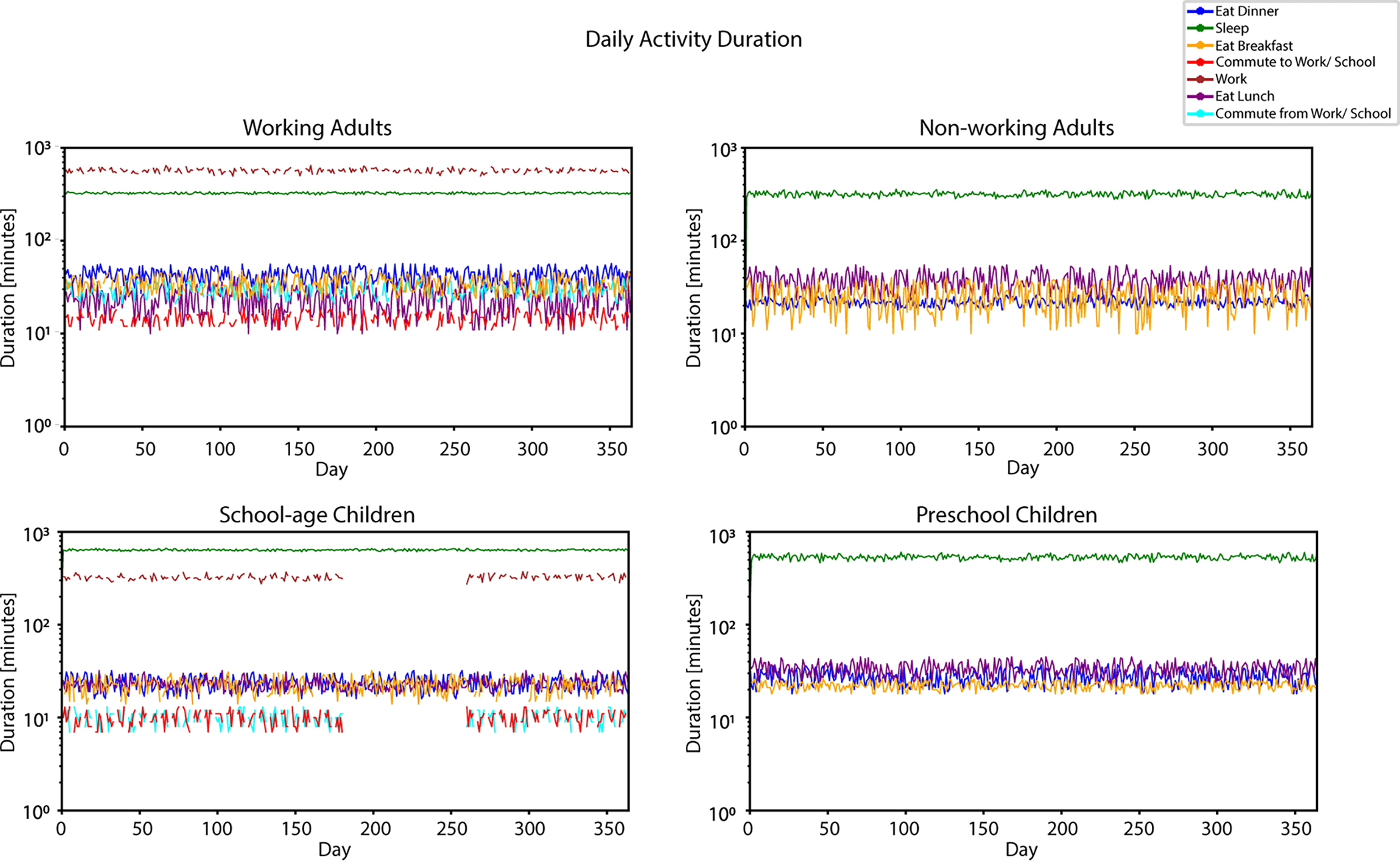
Visualization of example output of a full year of daily activity durations for all demographics. The durations are expressed in minutes in a log₁₀ scale

Figure 2.

Visualization of example output of two-weeks of daily activity durations for all demographics. The durations are expressed in minutes in a log₁₀ scale

The following analysis shows how distributions of the activity parameters from single-day ABMHAP output with and without consideration of intraindividual variation matches to single-day CHAD diaries (see Fig. 3). Figure 4 shows how the residuals of the quantile functions against the quantile rank for working adults with intraindividual variation. Residuals between ABMHAP without intraindividual variation and CHAD evaluation data are similar. Figures that describe ABMHAP’s performance with respect the other demographics may be found in Supplementary Figures 16 in the Supplementary Information. In addition, Table 10 summarizes ABMHAP’s performance for working adults by showing the mean of the absolute value of the residual function (seen in Fig. 4) for the middle 95% of the quantile range (we use the middle 95% to dismiss values from outliers). Numerical results that summarize ABMHAP’s performance for the other demographics may be found in Supplementary Tables 8–10.

Figure 3.

Cumulative distribution function (CDF) plots for activity start time, end time, and duration concerning working adults. (Blue) The distribution of ABMHAP predictions with intraindividual variation. (Black) The distribution of ABMHAP predictions without intraindividual variation. (Red) The distribution of single-day CHAD evaluation data

Figure 4.

The difference between the cumulative distribution functions (CDFs) between the CHAD single-day evaluation activity data and the corresponding ABMHAP predictions with intraindividual variation for working adults. The values are calculated by using Equation (1)

Table 10.

Mean absolute value of the middle 95% of residuals for working adults

Activity	Start [min]	End [min]	Duration [min]
Commute to work	6	7	1
Commute from work	15	14	1
Eat breakfast	48	48	4
Eat lunch	15	12	4
Eat dinner	6	4	3
Sleep	35	21	52
Work	10	7	18

DISCUSSION

From Fig. 1, one can see that working adults and school-age children are predicted to behave similarly; and nonworking adults and preschool children behave similarly as well. This is due to the presence/absence of the desire to go to work/school for the respective demographics. Since working adults and school-age children go to work/school, ABMHAP shows that these agents have less idle time than nonworking adults and preschool children. In addition, ABMHAP shows an example of seasonal changes in behavior for school-age children. For these agents, the break of the attending school and commuting activities is due to summer vacation, which occurs during the first 11 weeks of summer.

In Fig. 2, one can more clearly see the difference in behavior for working adults and school-age children due to a day being a weekday or weekend (i.e., these agents do not commute nor work/attend school on the weekend). In addition, the morning presents the possibility for these agents to simultaneously consider multiple unsatisfactory needs related to the activities: eat breakfast, commute to work/school, work/attend school. For these agents, sometimes breakfast is skipped. This can be seen in Fig. 2 as the absence of a duration for breakfast for some individuals on particular days. Breakfast may be skipped if the scheduled end time for sleep overlaps with the scheduled time to commute to work/school. Skipping breakfast may also occur if the end time for eating dinner overlaps the scheduled start time for sleep from the previous day. This causes the agent to start sleeping later and hence wake up later, which may cause the agent to skip breakfast. Either way, since the agent skips breakfast, the agent’s need to eat will be increasingly unsatisfied, causing the agent to eat lunch for a longer duration. Likewise, skipping dinner may occur if the agent ends the commute from work (school) sufficiently late and attempts to sleep sufficiently early before the scheduled dinner time.

The plots in Fig. 3 indicate that ABMHAP matches well with CHAD single-day records. This suggests that ABMHAP parameterized with longitudinal data mimics daily activity of working adults. Figure 4 shows the difference between ABMHAP output and randomly sampled CHAD data. For the most part, the residuals over the activity parameters distributions are small and indicate that ABMHAP is performing well in characterizing behavior observed in CHAD.

Table 10 shows that ABMHAP can match both the durations from CHAD in all activities and most of the start and end times. The biggest differences lie in ABMHAP’s ability to match the start times for both breakfast and sleep. This is due to our assumptions in how ABMHAP parameterizes the morning behavior. Namely, the agent’s expected behavior is to perform the following sequence without any idle time: wake up, eat breakfast, commute to work, and work. This assumption is an oversimplification of actual human behavior when people wake up in the morning; realistic behavior is more varied and is not captured by our assumptions. In addition, depending on the agent’s parameterization, the morning may lead to conflicts with sleeping and eating breakfast. Both factors may lead to inaccuracies seen in predicting the start time (and hence end time) for ABMHAP’s predictions for eating breakfast and sleeping. Nevertheless, ABMHAP parameterized with longitudinal data (where possible) can reasonably mimic CHAD single-day data over the simulated activities.

Figure 3 also shows that ABMHAP generates similar CDFs whether intraindividual variation is considered or not. This suggests the CHAD longitudinal records combined with our modeling assumptions show that human day-to-day behavior does not vary very much. Because these behaviors are driven by biological needs and the regular schedules of work/school, it is possible that the behaviors studied simulated in ABMHAP are more regular than other activities such as housecleaning or recreational activities [16].

Data on interindividual variation from longitudinal records are available for all behaviors. However, data on intraindividual variation are not available for parameterization due to an insufficient number of individuals with longitudinal activity patterns. This occurs for several behaviors in the four populations (see Tables 4–7). Using these data to both calibrate and to evaluate reduces the power of the analysis to evaluate the model’s predictions for intraindividual variation these behaviors. In these instances, we only assert that the analyses only demonstrate that ABMHAP produces internally-consistent predictions of intraindividual variation for these activities.

Table 4.

The number of unique individuals with CHAD records (single-day and longitudinal) for sleeping

Demographic group	Single-day records	Longitudinal records
Working adults	3909	779
Nonworking adults	2079	108
School-age children	2618	3764
Preschool children	703	0

We also acknowledge that there is a disconnection between a model of limited behaviors and the CHAD data. CHAD data reflect individuals performing many activities (child raising, exercise, and entertainment). As result, the CHAD data reflect decisions not included in ABMHAP. Nevertheless, ABMHAP can be made more robust by adding more behaviors than its current form. By doing so, the differences between limited models of behavior and empirical datasets could be investigated in the future.

ABMHAP provides increased benefits towards understanding human behavior for the exposure community. First, the use of behavioral data as input to ABMHAP may come not only from CHAD but also from other empirical data sources. Various human activity surveys, cell phone records, smart phones, and activity tracker devices like Fitbit may provide additional sources of human behavior data that could be used within the ABMHAP framework [17]. Second, additional benefits from ABMHAP come from its potential to support the modeling of longitudinal exposures to a wide range of environmental stressors [18,19,20,21,22]. For example, by defining commuting time, ABMHAP can generate estimates of exposure to traffic related air pollutants. Moreover, the time at home could be used to evaluate exposures to chemicals in indoor air. Likewise, since the use of most consumer products occurs during idle times, ABMHAP could provide a means of predicting when such products are used. Lastly, in the future ABMHAP could be extended to address more complex patterns of behavior such as child care, household cleaning and maintenance, entertainment, and social interactions between household members. To that end, we have made both the model code and the documentation available to the reader.

CONCLUSION

In this paper, we use the ABMHAP to simulate daily human activity. Through parameterizing ABMHAP with longitudinal data from the CHAD and evaluating ABMHAP with single-day data from CHAD, we show that ABMHAP can generate realistic longitudinal behavior patterns of sleeping, eating, commuting, working/attending school, and idle time (i.e., when an agent is not undergoing any of the aforementioned behaviors) for adults and children. In addition, the ability for ABMHAP to attain longitudinal behavior patterns will give exposure-assessors the ability to quickly generate rich human behavior data in ways not possible with current survey methods.

Table 2.

The number of unique individuals with CHAD records (single-day and longitudinal) for eating lunch

Demographic group	Single-day records	Longitudinal records
Working adults	1890	509
Nonworking adults	1560	576
School-age children	3463	1344
Preschool children	904	755

Table 3.

The number of unique individuals with CHAD records (single-day and longitudinal) for eating dinner

Demographic group	Single-day records	Longitudinal records
Working adults	2775	696
Nonworking adults	1852	803
School-age children	2585	3590
Preschool children	781	1132

Table 5.

The number of unique individuals with CHAD records (single-day and longitudinal) for working/attending school

Demographic group	Single-day records	Longitudinal records
Working adults	1347	4
School-age children	2168	286

Table 6.

The number of unique individuals with CHAD records (single-day and longitudinal) for commuting to work/school

Demographic group	Single-day records	Longitudinal records
Working adults	1513	4
School-age children	81	1

REFERENCES

- 1.Klepeis NE. An introduction to the indirect exposure assessment approach: modeling human exposure using microenvironmental measurements and the recent national human activity pattern survey. Environ Health Perspect. 1999;107:365–74. [DOI] [PMC free article] [PubMed] [Google Scholar]
- 2.Zartarian V, Xue J, Glen G, Smith L, Tulve N, Tornero-Velez R. Quantifying children’s aggregate (dietary and residential) exposure and dose to permethrin: application and evaluation of EPA’s probabilistic SHEDS-multimedia model. J Expo Sci Environ Epidemiol. 2012;22:267–73. [DOI] [PMC free article] [PubMed] [Google Scholar]
- 3.Egeghy PP, Quackenboss JJ, Catlin S, Ryan PB. Determinants of temporal variability in NHEXAS-Maryland. J Expo Anal Environ Epidemiol. 2005;15:388–97. [DOI] [PubMed] [Google Scholar]
- 4.Isaacs K, McCurdy T, Glen G, Nysewander M, Errickson A, Forbes S, et al. Statistical properties of longitudinal time-activity data for use in human exposure modeling. J Expo Sci Environ Epidemiol. 2013;23:328–36. [DOI] [PubMed] [Google Scholar]
- 5.Glen G, Smith L, Isaacs K, McCurdy T, Langstaff J. A New method of longitudinal diary assembly for human exposure modeling. J Expo Sci Environ Epidemiol. 2008;18:299–311. [DOI] [PubMed] [Google Scholar]
- 6.Graham SE, McCurdy T. Developing meaningful cohorts for human exposure models. J Expo Anal Environ Epidemiol. 2004;14:23–43. [DOI] [PubMed] [Google Scholar]
- 7.Xue J, McCurdy T, Spengler J, Özkaynak H. UnderStanding Variability in Time Spent in Selected Locations for 7–12-year old children. J Expo Anal Environ Epidemiol. 2014;14:222–33. [DOI] [PubMed] [Google Scholar]
- 8.Klepeis NE. Modeling human exposure to air pollution. In Ott WR, Steinemann AC, Wallace LA, editors. Exposure analysis. Boca Raton, Florida: CRC Press; 2006. p. 445–70. [Google Scholar]
- 9.Brandon N, Dionisio K, Isaacs K, Tornero-Velez R, Kapraun D, Setzer W, et al. Simulating exposure-related behaviors using agent-based models embedded with needs-based artificial intelligence. J Expo Sci Environl Epidemiol. 2018. 10.1038/s41370-018-0052-y. [DOI] [PMC free article] [PubMed] [Google Scholar]
- 10.Python Software Foundation. Python Software Foundation Website. https://www.python.org. Accessed 19 July 2017.
- 11.Zubek R Needs-based AI. In: Lake J, editor. Game Programming Gems 8. Boston, MA: Course Technology; 2011. p. 302–11. [Google Scholar]
- 12.Moya J, Phillips L, Schuda L, Wood P, Diaz A, Lee R.U.S. EPA et al. Exposure factors handbook. 2011. Washington, DC: U.S. Environmental Protection Agency; 2011. P. [Google Scholar]
- 13.United States Environmental Protection Agency. Consolidated Human Activity Database (CHAD) for use in human exposure and health studies and predictive models. https://www.epa.gov/healthresearch/consolidated-human-activity-database-chad-use-human-exposure-and-health-studies-and. Accessed Jan 2018.
- 14.McCurdy T, Glen G, Smith L, Lakkadi Y. The national exposure research laboratory’s consolidated human activity database. Int J Expo Anal Environ Epidemiol.2000;10:566–78. [DOI] [PubMed] [Google Scholar]
- 15.Isaacs KK, Glen WG, Egeghy P, Goldsmith MR, Smith L, Vallero D, et al. SHEDS-HT: an integrated probabilistic exposure model for prioritizing exposures to chemicals with near-field and dietary sources. Environ Sci Technol. 2014;48:12750–9. [DOI] [PubMed] [Google Scholar]
- 16.Wu X, Bennett DH, Lee K, Cassady DL, Ritz B, Hertz-Picciotto I. longitudinal variability of time-location/activity patterns of population at different ages: a longitudinal study in california. Environ Health. 2011; 10. 10.1186/1476-069X-10-80. [DOI] [PMC free article] [PubMed] [Google Scholar]
- 17.Fitbit. Fitbit. https://www.fitbit.com. Accessed 18 Apr 2018.
- 18.Rider CV, Dourson ML, Hertzberg RC, Mumtaz MM, Price PS, Simmons JE. Incorporating nonchemical stressors into cumalative risk assessments. Toxicol Sci. 2012;127:10–7. [DOI] [PMC free article] [PubMed] [Google Scholar]
- 19.Price PS, Chaisson CF. A conceptual framework for modeling aggregate and cumalative exposure to chemicals. J Expo Sci Environ Epidemiol. 2005;15:473–81. [DOI] [PubMed] [Google Scholar]
- 20.Hertz-Picciotto I, Cassady D, Lee K, Bennett DH, Ritz B, Vogt R. Study of use of products and exposure-related behaviors (SUPERB): study design, methods, and demographic characteristics of cohorts. Environ Health. 2010; 9. 10.1186/1476-069X-9-54. [DOI] [PMC free article] [PubMed] [Google Scholar]
- 21.Klepeis NE, Nelson WC, Ott WR, Robinson JP, Tsang AM, Switzer P, et al. The National Human Activity Pattern Survey (NHAPS): a resource for assessing exposure to environmental pollutants. J Expo Anal Environ Epidemiol. 2001;11:231–52. [DOI] [PubMed] [Google Scholar]
- 22.Zartarian VG, Xue J, Ozkaynak H, Dang W, Glen G, Smith L, et al. A probabilistic arsenic exposure assessment for children who contact CCA-treated playsets and decks, Part 1: model methodology, variability results, and model evaluation. Risk Anal. 2006;26:515–31. [DOI] [PubMed] [Google Scholar]
Associated Data
This section collects any data citations, data availability statements, or supplementary materials included in this article.