Mathematical assessment of monkeypox disease with the impact of vaccination using a fractional epidemiological modeling approach

Abstract

This present paper aims to examine various epidemiological aspects of the monkeypox viral infection using a fractional-order mathematical model. Initially, the model is formulated using integer-order nonlinear differential equations. The imperfect vaccination is considered for human population in the model formulation. The proposed model is then reformulated using a fractional order derivative with power law to gain a deeper understanding of disease dynamics. The values of the model parameters are determined from the cumulative reported monkeypox cases in the United States during the period from May 10th to October 10th, 2022. Besides this, some of the demographic parameters are evaluated from the population of the literature. We establish sufficient conditions to ensure the existence and uniqueness of the model’s solution in the fractional case. Furthermore, the stability of the endemic equilibrium of the fractional monkeypox model is presented. The Lyapunov function approach is used to demonstrate the global stability of the model equilibria. Moreover, the fractional order model is numerically solved using an efficient numerical technique known as the fractional Adams-Bashforth-Moulton method. The numerical simulations are conducted using estimated parameters, considering various values of the fractional order of the Caputo derivative. The finding of this study reveals the impact of various model parameters and fractional order values on the dynamics and control of monkeypox.

Introduction

Monkeypox is a viral disease caused by the monkeypox virus (MPXV), which belongs to the Orthopoxvirus genus. It primarily affects animals, particularly monkeys, squirrels, and rodents. It is a zoonotic disease that can be transmitted to humans through animals. Human-to-human transmission can also occur via close contact with infected individuals, particularly through respiratory droplets or contact with skin lesions or other body fluids. Besides these, other possible modes of transmission include contact with contaminated objects or surfaces known as environmental transmission. Although, infected cases are found in numerous countries in the world, but Africa is the main place where it is most commonly found. The first monkeypox case was identified in 1958 following the occurrence of outbreaks in a group of monkeys that were being studied. Globally, there have been a total of 88,122 reported cases of infection, with 30,555 of these cases occurring in the United States¹. The symptoms of monkeypox virus infection in humans are comparable to smallpox signs but less severe^2,3. Typically, the infection begins with a fever, headache, muscle pain, and tiredness³. The primary distinction between the symptoms of monkeypox and smallpox is that the monkeypox infection results in lymphadenopathy, characterized by the swelling of lymph nodes³. The incubation period for this infection usually ranges from 7 to 14 days, although it can vary between 5 and 21 days^1,3. Symptoms of monkeypox are usually mild, and the majority of patients naturally recover within a few weeks. Those with weakened immune systems may exhibit severe symptoms^1,2,4,5. Smallpox and human monkeypox are clinically related due to their difficult-to-distinguish characteristics². Typically, monkeypox is spread to humans through contact with animal blood or bites from rodents, pets, and primates^2,3. Gambian pouched rats (Cricetomys Gambians), dormice (Graphiurus sp.), and African squirrels (Heliosciurus and Funisciurus) have also been found to be infected⁴. Currently, no approved and safe treatment mechanism specifically for monkeypox virus infection. Nevertheless, some particular controlling measures can be used to mitigate the spread of monkeypox. Vaccines, immune globulin, and antiviral medications introduced for smallpox control can be employed to control the transmission. However, that the smallpox vaccine is currently unavailable as smallpox has been eradicated worldwide^6,7.

Monkeypox has received little attention in the past, making it difficult to understand its epidemiology. Despite this, numerous mathematical models have been recently developed to analyze the dynamics of the monkeypox. A novel mathematical model based on deterministic approach for the monkeypox outbreak was developed and examined in⁸. Their findings revealed that isolating infected people from other populations reduces disease incidence. In⁹ the authors developed a system of nonlinear differential equations to analyze different modes of monkeypox transmission. The numerical simulation indicates that the immunological status of an individual affects how well they recover from an orthopoxvirus infection. To learn more about the mechanisms of transmission and various controlling methods, many epidemic models on infectious disease have been investigated^8,10–13. In¹⁴ authors developed a mathematical model to better comprehend the dynamics of the monkeypox. Their results suggest the monkeypox outbreak can be eradicated through the proper implementation of non-pharmaceutical interventions. Additionally, in the study of¹⁵, the numerical simulation of the model demonstrated that the treatment will result in the elimination of infected individuals from human and non-human primate populations throughout the course of the investigation. Recently, in^16,17 the authors introduce a mathematical model with environmental transmission to study the dynamics and some controlling measures of the monkeypox 2022 outbreak.

Mathematical modeling with fractional differential equations has recently attracted the attention of researchers in a wide range of scientific and professional domains, particularly in epidemiology^18–20. The memory effect is one of the remarkable characteristics of fractional-order models that cannot be developed in classical models because of the numerous properties of fractional operators^21,22. Many researchers have recently employed fractional differential equations to represent a variety of infectious and non-infectious diseases. One of these study subjects that has received great attention and produced insightful results is the COVID-19 infection. Mathematical models for COVID-19 based on the fractional derivatives are taken into account in^23–27. The dynamics of monkeypox with cross-infection via a novel stochastic model was studied in²⁸. A novel modeling approach based on fractal-fractional operators demonstrating monkeying dynamics with animal-to-human transmission was proposed in²⁹.

This study analyzes the dynamics of monkeypox under some controlling measures using fractional-order calculus. We present a comprehensive theoretical and numerical analysis of the fractional order epidemic model. Most of the model parameters are estimated from the actual data set of the monkeypox 2022 outbreak. The description of the manuscript’s main sections is as follows: The section titled “Basic definitions” introduces some fundamental concepts of fractional derivatives. The proposed monkeypox model and parameter estimation are described in section “Formulation of the integer order monkeypox model”. The model’s qualitative analysis is presented in section “Basic analysis of the fractional monkeypox model”. A graphical interpretation of the basic reproduction number versus model parameters is presented in section “Interpretations of ${\mathcal{R}}_0$ versus model parameters”. Detailed numerical treatment for the fractional model is accomplished in section “Numerical results of the fractional model”. Finally, in the last section titled “Conclusion,” we summarized with a conclusion.

Basic definitions

Fractional differential operators in mathematical modeling are well-known and it has been successful in the fields like science, engineering, and epidemiology. We give a few fundamental definitions along with some proprieties that be will used in the rest of the study^30,31.

Definition 1

The left and right Caputo fractional derivative operator of the function $f\in L^{\infty }(\mathbb{R})\cap C(\mathbb{R})$ is defined as follows

$$\begin{array}{cc}& {}_{t_0}^c{D}_t^{\vartheta }f\left(t\right)=\left({}_{t_0}{D}_t^{-\left(m-\vartheta \right)}{\left(\frac{d}{\mathit{dt}}\right)}^{m}f\left(t\right)\right)=\frac{1}{\mathrm{\Gamma }\left(m-\vartheta \right)}\underset{t_0}{\overset{t}{\int }}\left({\left(t-l\right)}^{m-\vartheta -1}{f}^m\left(l\right)\right)dl,\hfill \\ \hfill & \mathit{and}\hfill \\ \hfill & {}_t^c{D}_T^{\vartheta }f\left(t\right)=\left({}_t{D}_T^{-\left(m-\vartheta \right)}{\left(-\frac{d}{\mathit{dt}}\right)}^{m}f\left(t\right)\right)=\frac{{\left(-1\right)}^m}{\mathrm{\Gamma }\left(m-\vartheta \right)}\underset{t}{\overset{T}{\int }}\left({\left(l-t\right)}^{m-\vartheta -1}{f}^m\left(l\right)\right)dl.\hfill \end{array}$$ 1

Definition 2

For $x\in \mathbb{R}$, the generalized Mittag-Leffler function $E_{\alpha ,\beta }(x)$ is defined by

$$\begin{array}{c}\hfill E_{\alpha ,\beta }\left(x\right)=\sum _{m=0}^{\infty }\frac{x^m}{\mathrm{\Gamma }\left(\alpha m+\beta \right)},\alpha ,\beta >0,\end{array}$$ 2

and satisfies the following property given in

$$\begin{array}{c}\hfill E_{\alpha ,\beta }\left(x\right)=x{E}_{\alpha ,\alpha +\beta }\left(x\right)+\frac{1}{\mathrm{\Gamma }\left(\beta \right)}.\end{array}$$ 3

The Laplace transform of the function $t^{\beta -1}{E}_{\alpha ,\beta }\left(\pm \lambda t^{\alpha }\right)$ is defined as follows

$$\begin{array}{c}\hfill L\left[t^{\beta -1}{E}_{\alpha ,\beta }\left(\pm \lambda t^{\alpha }\right)\right]=\frac{s^{\alpha -\beta }}{s^{\alpha }\mp \lambda }.\end{array}$$ 4

Proposition 2.1

Let, $f\in L^{\infty }(\mathbb{R})\cap C(\mathbb{R})$ and $\alpha \in \mathbb{R}$, $m-1<\alpha <m$ then the following condition hold

$$\begin{array}{cc}\hfill & 1.{}_{t_0}^c{D}_t^{\vartheta }{I}^{\vartheta }f\left(t\right)=f\left(t\right).\hfill \\ \hfill & 2.I^{\vartheta }{}_{t_0}^c{D}_t^{\vartheta }f\left(t\right)=f\left(t\right)-\sum _{k=0}^{m-1}\frac{t^k}{k!}{f}^k\left(t_0\right).\hfill \end{array}$$

Formulation of the integer order monkeypox model

The total human population $N_h$ is divided into six different compartments i.e $S_h$ susceptible humans, $E_h$ exposed humans, $I_h$ infected humans, $C_h$ clinically ill humans, $V_h$ vaccinated humans and $R_h$ recovered individuals. Similarly, $N_r$ represents the overall non-human population which is further divided into four different subgroups i.e. $S_r$ susceptible, $E_r$ exposed, $I_r$ infected and $R_r$ recovered animals respectively.

The susceptible human class is initiated through recruited rate ${\varphi }_h$. This population is declined by the natural mortality rate ${\mu }_h$ and by the population gaining infection after interacting with infected humans (or animals) at the contact rate ${\beta }_1$ or ${\beta }_2$ respectively. The susceptible human group is also decreased by vaccinating at the rate ${\alpha }_h$. This class is further increased by the vaccinated population after waning the induced immunity at the rate $\eta$. Thus, the dynamics of the susceptible human class are modeled via the following equation

$$\begin{array}{c}\hfill \frac{d{S}_h}{\mathit{dt}}={\varphi }_h-\left(\frac{{\beta }_1{I}_h+{\beta }_2{I}_r}{N_h}\right)S_h-\left({\mu }_h+{\alpha }_h\right)S_h+\eta V_h.\end{array}$$

The class of exposed individuals is increased by joining the newly infected individuals with the force of infection ${\lambda }_h=\left(\frac{{\beta }_1{I}_h+{\beta }_2{I}_r}{N_h}\right)$. Moreover, this population class is declined by the transmission rate $\beta$ and the mortality rate ${\mu }_h$. Thus, we obtained the following differential equation describing the dynamics of exposed human class

$$\begin{array}{c}\hfill \frac{d{E}_h}{\mathit{dt}}=\left(\frac{{\beta }_1{I}_h+{\beta }_2{I}_r}{N_h}\right)S_h-\left({\mu }_h+\beta \right)E_h.\end{array}$$

The number of infected people rises at a rate of $\beta$ after the transition from being exposed class. This class is decreased by the natural death rate ${\mu }_h$, the disease-induced death rate ${\delta }_1$, the recovered population at the ${\omega }_1$ and by the people who became clinically ill and join next class at the rate $\gamma$. Thus, the resulting dynamics can be modeled via the following equation

$$\begin{array}{c}\hfill \frac{d{I}_h}{\mathit{dt}}=\beta E_h-\left({\omega }_1+\gamma +{\mu }_h+{\delta }_1\right)I_h.\end{array}$$

The people in $I_h$ class become clinically (or critically) ill at the rate $\gamma$ and join $C_h$ class. These individuals are reduced by natural mortality rate ${\mu }_h$ and disease-induced death rate ${\delta }_2$. Further, it is decreased by joining the recovered class at the rate $\rho$. Hence, we obtained the following equation describing the dynamics of $C_h$ population

$$\begin{array}{c}\hfill \frac{d{C}_h}{\mathit{dt}}=\gamma I_h-\left(\rho +{\mu }_h+{\delta }_2\right)C_h.\end{array}$$

The susceptible individuals are vaccinated at the rate ${\alpha }_h$. The vaccinated individuals are decreased due to natural mortality rate ${\mu }_h$ and due to the waning of induced immunity at a rate $\eta$. Thus, we have

$$\begin{array}{c}\hfill \frac{d{V}_h}{\mathit{dt}}={\alpha }_h{S}_h-({\mu }_h+\eta )V_h.\end{array}$$

Finally, the class of recovered humans is formed due to the transition of individuals from $I_h$ and $C_h$ at the recovery rates $\rho$ and ${\omega }_1$ respectively. Further, it is decreased due to the natural death rate ${\mu }_h$. Thus, we obtain

$$\begin{array}{c}\hfill \frac{d{R}_h}{\mathit{dt}}=\rho C_h+{\omega }_1{I}_h-{\mu }_h{R}_h.\end{array}$$

The recruitment rate of susceptible animals is ${\varphi }_r$ and the natural death rate in all animal populations is denoted by ${\mu }_r$. The force of infection in this case is given by

$$\begin{array}{c}\hfill {\lambda }_r=\frac{{\beta }_3{I}_r}{N_r},\end{array}$$

where ${\beta }_3$ is the effective contact rate causing the disease transmission rate among animals. The flow from exposed to the infected animal compartment is denoted by $\epsilon$. The death rate induced due to infection in infected animals is ${\delta }_3$. The parameter ${\omega }_2$ shows the recovery rate of infected animals. Thus, the dynamics of monkeypox in animals are given by the following system

$$\begin{array}{cc}\hfill \frac{d{S}_r}{\mathit{dt}}=& {\varphi }_r-\left(\frac{{\beta }_3{I}_r}{N_r}\right)S_r-{\mu }_r{S}_r,\hfill \\ \hfill \frac{d{E}_r}{\mathit{dt}}=& \left(\frac{{\beta }_3{I}_r}{N_r}\right)S_r-\left(\epsilon +{\mu }_r\right)E_r,\hfill \\ \hfill \frac{d{I}_r}{\mathit{dt}}=& \epsilon E_r-\left({\omega }_2+{\mu }_h+{\delta }_3\right)I_r,\hfill \\ \hfill \frac{d{R}_r}{\mathit{dt}}=& {\omega }_2{I}_r-{\mu }_r{R}_r.\hfill \end{array}$$ 5

Fractional monkeypox model in the Caputo sense

This section presents the extension of the integer order monkeypox model to the fractional case. The well-known Caputo derivative having order $0<\vartheta \le 1$ is utilized to formulate the generalized fractional epidemic model. Fractional epidemic models used fractional derivatives to capture more complex and non-local effects in the disease transmission dynamics. Such epidemic models have a greater degree of freedom and offer insights into the behavior and control of infectious diseases for a particular set of data²². The proposed model for transmission of monkeypox model is described by the following system

$$\begin{array}{cc}\hfill {}^c{D}_t^{\vartheta }{S}_h=& {\varphi }_h-{\lambda }_h{S}_h-{\mathtt{k}}_1{S}_h+\eta V_h,\hfill \\ \hfill {}^c{D}_t^{\vartheta }{E}_h=& {\lambda }_h{S}_h-{\mathtt{k}}_2{E}_h,\hfill \\ \hfill {}^c{D}_t^{\vartheta }{I}_h=& \beta E_h-{\mathtt{k}}_3{I}_h,\hfill \\ \hfill {}^c{D}_t^{\vartheta }{C}_h=& \gamma I_h-{\mathtt{k}}_4{C}_h,\hfill \\ \hfill {}^c{D}_t^{\vartheta }{V}_h=& {\alpha }_h{S}_h-{\mathtt{k}}_5{V}_h,\hfill \\ \hfill {}^c{D}_t^{\vartheta }{R}_h=& \rho C_h+{\omega }_1{I}_h-{\mu }_h{R}_h,\hfill \\ \hfill {}^c{D}_t^{\vartheta }{S}_r=& {\varphi }_r-\left({\lambda }_r+{\mu }_r\right)S_r,\hfill \\ \hfill {}^c{D}_t^{\vartheta }{E}_r=& {\lambda }_r{S}_r-{\mathtt{k}}_6{E}_r,\hfill \\ \hfill {}^c{D}_t^{\vartheta }{I}_r=& \epsilon E_r-{\mathtt{k}}_7{I}_r,\hfill \\ \hfill {}^c{D}_t^{\vartheta }{R}_r=& {\omega }_2{I}_r-{\mu }_r{R}_r,\hfill \end{array}$$ 6

where,

$$\begin{array}{cc}\hfill {\mathtt{k}}_1& =\left({\mu }_h+{\alpha }_h\right),{\mathtt{k}}_2=\left({\mu }_h+\beta \right),{\mathtt{k}}_3=\left({\omega }_1+\gamma +{\mu }_h+{\delta }_1\right),{\mathtt{k}}_4=\left(\delta +{\mu }_h+{\delta }_2\right),{\mathtt{k}}_5=\left({\mu }_h+\eta \right),\hfill \\ \hfill {\mathtt{k}}_6& =\left(\epsilon +{\mu }_r\right){\mathtt{k}}_7=\left({\omega }_2+{\mu }_h+{\delta }_3\right).\hfill \end{array}$$

Subject to non-negative initial conditions

$$\begin{array}{cc}\hfill S_h\left(0\right)=& {\stackrel{⌣}{S}}_{h_0},E_h\left(0\right)={\stackrel{⌣}{E}}_{h_0},I_h\left(0\right)={\stackrel{⌣}{I}}_{h_0},C_h\left(0\right)={\stackrel{⌣}{C}}_{h_0},V_h\left(0\right)={\stackrel{⌣}{V}}_{h_0},R_h\left(0\right)={\stackrel{⌣}{R}}_{h_0},\hfill \\ \hfill S_r\left(0\right)=& {\stackrel{⌣}{S}}_{r_0},E_r\left(0\right)={\stackrel{⌣}{E}}_{r_0},I_r\left(0\right)={\stackrel{⌣}{I}}_{r_0}and{R}_r\left(0\right)={\stackrel{⌣}{R}}_{r_0}.\hfill \end{array}$$ 7

Parameter estimation and data fitting

The objective of the present section is to accomplish the parameter estimation of the model. The estimation procedure is performed in two ways. Most of the model parameters are estimated from the real statistics of infected cases reported from 10 May to the end of October 2022 in the recent outbreak in the USA^1,3. While some of the demographic parameters (the natural death and birth rate) are estimated from the USA population³². The estimation of parameters from the real disease data is significant for carrying out the numerical simulations more realistically. The estimation process of the proposed model (6) is conducted using the well-known nonlinear least square technique.

This procedure involves the following main steps:

1. Define an objective function for quantifying the difference between the predicted and the actual data. This function is mathematically expressed as the sum of squared residuals (SSR) between the model predictions and the corresponding actual data points.

2. Define or set the model parameters’ initial values that need to be estimated. These values can be based on prior knowledge or initial guesses.

3. Utilizing the initial parameter values set in step 2, the epidemic model is simulated in order to generate model predictions.

4. Using a ’lsqcurvefit’ optimization technique, for the minimization of objective function.

5. Set a convergence criterion to stop the iterative estimation scheme. This criterion is based on a maximum number of iterations, a minimal change in parameter estimates, or attaining a predefined threshold for the corresponding objective function.

6. If the estimated parameter values do not adequately fit the real data curve or do not meet the convergence criterion, reset the initial parameter estimates and re-execute steps 3–5 until a reasonable agreement between the model simulation and the actual data is obtained.

By iteratively minimizing the objective function via a standard nonlinear least squares technique, the parameter estimates are refined, which leads to improved agreement between the model-predicted and observed data. The fitted and estimated values of the monkeypox epidemic model’s parameters are listed in Table 1, while Fig. 1 illustrates the model’s good fit to the observed data.

Table 1.

Fitted and estimated values of the model parameters.

Parameter	Description	Value in days	References
${\varphi }_h$	Birth rate of humans	11731.91	32
${\varphi }_r$	Birth rate of animals or rodents	0.016	8
$\eta$	Waning induced immunity	0.2010	Fitted
$\rho$	Recovery rate of $C_h$	0.0843	Fitted
$\beta$	Transition rate of $E_h$ to $I_h$	0.0486	Fitted
$\gamma$	Moving of $I_h$ to $C_h$	0.1119	Fitted
${\beta }_3$	Contact rate of $S_r$ and $I_r$	0.2461	Fitted
${\beta }_1$	Contact rate of $S_h$ and $I_h$	0.5701	Fitted
${\beta }_2$	Contact rate between $I_r$ and $S_h$	0.2508	Fitted
${\alpha }_h$	Vaccinated against monkeypox	0.2393	Fitted
${\mu }_h$	Natural death rate of humans	1/(79*365)	32
${\delta }_1$	Disease induced mortality rate of infectious human	0.0011	Fitted
${\delta }_2$	Disease-induced rate of $C_h$	1.0091e−04	Fitted
${\delta }_3$	Disease induced death rate of infected animals	1.5303e−05	Fitted
${\omega }_1$	Permanent immunity due to treatment	0.4670	Fitted
${\mu }_r$	Natural death rate of animals	0.000016	8
${\omega }_2$	Recovery rate due to immunity	0–1	Assumed
$ϵ$	Progression from being $E_r$ to $I_r$	0.1053	Fitted

Figure 1.

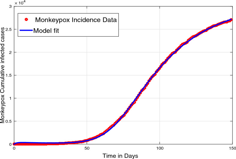
Model predicted curve (solid line) to the observed data for the case when $\vartheta =1$.

Basic analysis of the fractional monkeypox model

In this section, we address some of the basic and necessary mathematical analysis of the fractional monkeypox epidemic model (6). We proceed as follows

Positivity and boundedness

For the positive initial values $\underset{t\to \infty }{lim}sup{N}_h\left(t\right)\le \frac{{\varphi }_h}{{\mu }_h}and\underset{t\to \infty }{lim}sup{N}_r\left(t\right)\le \frac{{\varphi }_r}{{\mu }_r}$. Also, if $N_{h_0}\left(t\right)\le \frac{{\varphi }_h}{{\mu }_h}and{N}_{r_0}\left(t\right)\le \frac{{\varphi }_r}{{\mu }_r}$ then the feasible domain for the given system is given by

$$\begin{array}{cc}\hfill {\mathrm{\Omega }}_h& =\left\{\left(S_h,E_h,I_h,C_h,V_h,R_h\right)\subset {\mathbb{R}}_{+}^6:S_h+E_h+I_h+C_h+V_h+R_h\le \frac{{\varphi }_h}{{\mu }_h}\right\},\hfill \\ \hfill {\mathrm{\Omega }}_r& =\left\{\left(S_r,E_r,I_r,R_r\right)\subset {\mathbb{R}}_{+}^4:S_r+E_r+I_r+R_r\le \frac{{\varphi }_r}{{\mu }_r}\right\},\hfill \\ \hfill \end{array}$$

such that $\mathrm{\Omega }={\mathrm{\Omega }}_h\times {\mathrm{\Omega }}_r\subset {\mathbb{R}}_{+}^6\times {\mathbb{R}}_{+}^4$ and we have $\mathrm{\Omega }$ is positively invariant.

Let ${\stackrel{⌣}{S}}_{h_0}{\stackrel{⌣}{E}}_{h_0},{\stackrel{⌣}{I}}_{h_0},{\stackrel{⌣}{C}}_{h_0},{\stackrel{⌣}{V}}_{h_0},{\stackrel{⌣}{R}}_{h_0},$ ${\stackrel{⌣}{S}}_{r_0},{\stackrel{⌣}{E}}_{r_0},{\stackrel{⌣}{I}}_{r_0}$ and ${\stackrel{⌣}{R}}_{r_0}$ be positive, then all solution are will be positive for $t>0$. Considering the first equation in (6) we have

$$\begin{array}{c}\hfill {}^c{D}_t^{\vartheta }{S}_h={\varphi }_h-\left({\lambda }_h+{\mathtt{k}}_1\right)S_h+\eta V_h,\end{array}$$

then

$$\begin{array}{c}\hfill {}^c{D}_t^{\vartheta }{S}_h+\left({\lambda }_h+{\mathtt{k}}_1\right)S_h={\varphi }_h+\eta V_h.\end{array}$$

Since ${\varphi }_h+\eta V_h\ge 0$ therefore, it implies

$$\begin{array}{c}\hfill {}^c{D}_t^{\vartheta }{S}_h+\left({\lambda }_h+{\mathtt{k}}_1\right)S_h\ge 0.\end{array}$$

By using the Laplace transform we have

$$\begin{array}{cc}& L\left[{}^c{D}_t^{\vartheta }{S}_h\right]+L\left[\left({\lambda }_h+{\mathtt{k}}_1\right)S_h\right]\ge 0,\hfill \\ \hfill & s^{\vartheta }{S}_h\left(s\right)-s^{\vartheta -1}{S}_h\left(0\right)+\left({\lambda }_h+{\mathtt{k}}_1\right)S_h\left(s\right)\ge 0,\hfill \\ \hfill & S_h\left(s\right)\ge \frac{s^{\vartheta -1}}{\left(s^{\vartheta }+\left({\lambda }_h+{\mathtt{k}}_1\right)\right)}{S}_{h_0}.\hfill \end{array}$$

Applying inverse Laplace transform we have

$$\begin{array}{c}\hfill S_h\left(t\right)\ge E_{\vartheta ,1}\left(-\left({\lambda }_h+{\mathtt{k}}_1\right)t^{\vartheta }\right)S_{h_0}.\end{array}$$

Since, quantities on right hand side are positive so we have $S_h\ge 0$ for $t\ge 0$. In similar approach, we have $E_h,I_h,C_h,V_h,R_h,S_r,E_r,I_{r}and{R}_r\ge 0\forall t>0$ corresponding to any non-negative initial values. Thus, the solution remain in ${\mathbb{R}}_{+}^6\times {\mathbb{R}}_{+}^4$ for all $t>0$ with non-negative initial values.

Next to we prove the boundedness of the fractional model solution. The total human individuals is given by

$$\begin{array}{c}\hfill N_h\left(t\right)=S_h\left(t\right)+E_h\left(t\right)+I_h\left(t\right)+C_h\left(t\right)+V_h\left(t\right)+R_h\left(t\right),\end{array}$$

such that

$$\begin{array}{cc}\hfill {}^c{D}_t^{\vartheta }{N}_h\left(t\right)& {=}^c{D}_t^{\vartheta }{S}_h\left(t\right){+}^c{D}_t^{\vartheta }{E}_h\left(t\right){+}^c{D}_t^{\vartheta }{I}_h\left(t\right){+}^c{D}_t^{\vartheta }{C}_h\left(t\right){+}^c{D}_t^{\vartheta }{V}_h\left(t\right){+}^c{D}_t^{\vartheta }{R}_h\left(t\right),\hfill \\ \hfill {}^c{D}_t^{\vartheta }{N}_h\left(t\right)& ={\varphi }_h-\left({\delta }_1{I}_h+{\delta }_2{C}_h\right)-{\mu }_h{N}_h\left(t\right)\le {\varphi }_h-{\mu }_{h}N\left(t\right),\hfill \\ \hfill {}^c{D}_t^{\vartheta }{N}_h\left(t\right)& \le {\varphi }_h-{\mu }_h{N}_h\left(t\right).\hfill \end{array}$$

Taking Laplace transform on both sides we have

$$\begin{array}{cc}& L\left[{}^c{D}_t^{\vartheta }{N}_h\left(t\right)\right]\le L\left[{\varphi }_h-{\mu }_h{N}_h\left(t\right)\right],\hfill \\ \hfill & s^{\vartheta }{N}_h\left(s\right)-s^{\vartheta -1}{N}_h\left(0\right)+{\mu }_h{N}_h\left(s\right)\le \frac{{\varphi }_h}{s},\hfill \\ \hfill & N_h\left(s\right)\le \frac{s^{\vartheta -1}}{\left(s^{\vartheta }+{\mu }_h\right)}{N}_h\left(0\right)+\frac{{\varphi }_h}{s\left(s^{\vartheta }+{\mu }_h\right).}\hfill \end{array}$$

By applying inverse Laplace transform we have

$$\begin{array}{c}\hfill N_h\left(t\right)\le E_{\vartheta ,1}\left(-{\mu }_h{t}^{\vartheta }\right)N_h\left(0\right)+{\varphi }_h{E}_{\vartheta ,\vartheta +1}\left(-{\mu }_h{t}^{\vartheta }\right).\end{array}$$ 8

By taking limit $t\to \infty$ we have $N_h(t)\le \frac{{\varphi }_h}{{\mu }_h}$ implies that $\underset{t\to \infty }{lim}sup{N}_h\left(t\right)=\frac{{\varphi }_h}{{\mu }_h}.$ If $N_{h_0}\le \frac{{\varphi }_h}{{\mu }_h}$ then $N_h\left(t\right)\le \frac{{\varphi }_h}{{\mu }_h}$ which implies $N_h(t)$ is bounded. In similar way, we can prove that $N_r(t)$ is bounded. Therefore, this established the notion of the set $\mathrm{\Omega }$ as required. So, we conclude that the region is epidemiological feasible and well posed in $\mathrm{\Omega }$.

Existence and uniqueness

Let T be a positive real number and consider $J=[0,T]$. We denote the set of all continuous function defined on J by $C_e^0(J)$ with norm as $∥X∥=sup\left\{\left|X\left(t\right)\right|,t\in J\right\}.$ Consider the system (6), (7) as following initial value problem (I.V.P.)

$$\begin{array}{c}\hfill \left\{\begin{array}{c}{}^c{D}_t^{\vartheta }X\left(t\right)=F\left(t,X\left(t\right)\right),0<t<T<\infty ,\hfill \\ X\left(0\right)=X_0,\hfill \end{array}\right)\end{array}$$ 9

where $X(t)=(S_h(t),E_h(t),I_h(t),C_h(t),V_h(t),R_h(t),S_r(t),E_r(t),I_r(t),R_r(t))$ represents the compartments and F is continuous function defined as follows

$$\begin{array}{c}\hfill F\left(t,X\left(t\right)\right)=\left(\begin{array}{c}{F}_1\left(t,S_h\left(t\right)\right)\hfill \\ F_2\left(t,E_h\left(t\right)\right)\hfill \\ F_3\left(t,I_h\left(t\right)\right)\hfill \\ F_4\left(t,C_h\left(t\right)\right)\hfill \\ F_5\left(t,V_h\left(t\right)\right)\hfill \\ F_6\left(t,R_h\left(t\right)\right)\hfill \\ F_7\left(t,S_r\left(t\right)\right)\hfill \\ F_8\left(t,E_r\left(t\right)\right)\hfill \\ F_9\left(t,I_r\left(t\right)\right)\hfill \\ F_{10}\left(t,R_r\left(t\right)\right)\hfill \end{array}\right)=\left(\begin{array}{c}{\varphi }_h-\left(\frac{{\beta }_1{I}_h+{\beta }_2{I}_r}{N_h}+{\mu }_h\right)S_h-{\alpha }_h{S}_h+\eta V_h\hfill \\ \left(\frac{{\beta }_1{I}_h+{\beta }_2{I}_r}{N_h}\right)S_h-\left({\mu }_h+\beta \right)E_h\hfill \\ \beta E_h-\left({\omega }_1+\gamma +{\mu }_h+{\delta }_1\right)I_h\hfill \\ \gamma I_h-\left(\rho +{\mu }_h+{\delta }_2\right)C_h\hfill \\ {\alpha }_h{S}_h-{\mu }_h{V}_h-\eta V_h\hfill \\ \rho C_h+{\omega }_1{I}_h-{\mu }_h{R}_h\hfill \\ {\varphi }_r-\left(\frac{{\beta }_3{I}_r}{N_r}+{\mu }_r\right)S_r\hfill \\ \left(\frac{{\beta }_3{I}_r}{N_r}\right)S_r-\left(\epsilon +{\mu }_r\right)E_r\hfill \\ \epsilon E_r-\left({\mu }_r+{\delta }_3+{\omega }_2\right)I_r\hfill \\ {\omega }_2{I}_r-{\mu }_r{R}_r\hfill \end{array}\right).\end{array}$$ 10

Using property (2.1) in proposition we have

$$\begin{array}{cc}\hfill S_h\left(t\right)& ={\stackrel{⌣}{S}}_{h_0}+I_t^{\vartheta }\left({\varphi }_h-\left(\frac{{\beta }_1{I}_h+{\beta }_2{I}_r}{N_h}+{\mu }_h\right)S_h-{\alpha }_h{S}_h+\eta V_h\right),\hfill \\ \hfill \\ \hfill E_h\left(t\right)& ={\stackrel{⌣}{E}}_{h_0}+I_t^{\vartheta }\left(\left(\frac{{\beta }_1{I}_h+{\beta }_2{I}_r}{N_h}\right)S_h-\left({\mu }_h+\beta \right)E_h\right),\hfill \\ \hfill \\ \hfill I_h\left(t\right)& ={\stackrel{⌣}{I}}_{h_0}+I_t^{\vartheta }\left(\beta E_h-\left({\omega }_1+\gamma +{\mu }_h+{\delta }_1\right)I_h\right),\hfill \\ \hfill \\ \hfill C_h\left(t\right)& ={\stackrel{⌣}{C}}_{h_0}+I_t^{\vartheta }\left(\gamma I_h-\left(\rho +{\mu }_h+{\delta }_2\right)C_h\right),\hfill \\ \hfill \\ \hfill V_h\left(t\right)& ={\stackrel{⌣}{V}}_{h_0}+I_t^{\vartheta }\left({\alpha }_h{S}_h-{\mu }_h{V}_h-\eta V_h\right),\hfill \\ \hfill \\ \hfill R_h\left(t\right)& ={\stackrel{⌣}{R}}_{h_0}+I_t^{\vartheta }\left(\rho C_h+{\omega }_1{I}_h-{\mu }_h{R}_h\right),\hfill \\ \hfill \\ \hfill S_r\left(t\right)& ={\stackrel{⌣}{S}}_{r_0}+I_t^{\vartheta }\left({\varphi }_r-\left(\frac{{\beta }_3{I}_r}{N_r}+{\mu }_r\right)S_r\right),\hfill \\ \hfill \\ \hfill E_r\left(t\right)& ={\stackrel{⌣}{E}}_{r_0}+I_t^{\vartheta }\left(\left(\frac{{\beta }_3{I}_r}{N_r}\right)S_r-\left(\epsilon +{\mu }_r\right)E_r\right),\hfill \\ \hfill \\ \hfill I_r\left(t\right)& ={\stackrel{⌣}{I}}_{r_0}+I_t^{\vartheta }\left(\epsilon E_r-\left({\mu }_r+{\delta }_3+{\omega }_2\right)I_r\right),\hfill \\ \hfill \\ \hfill R_r\left(t\right)& ={\stackrel{⌣}{R}}_{r_0}+I_t^{\vartheta }\left({\omega }_2{I}_r-{\mu }_r{R}_r\right).\hfill \\ \hfill \end{array}$$

The Picard iterations lead as follows

$$\begin{array}{cc}\hfill S_{h_n}\left(t\right)& ={\stackrel{⌣}{S}}_{h_0}+\frac{1}{\mathrm{\Gamma }\left(\vartheta \right)}\underset{0}{\overset{t}{\int }}{\left(t-l\right)}^{\vartheta -1}{F}_1\left(l,S_{h_{n-1}}\left(l\right)\right)dl,\hfill \\ \hfill \\ \hfill E_{h_n}\left(t\right)& ={\stackrel{⌣}{E}}_{h_0}+\frac{1}{\mathrm{\Gamma }\left(\vartheta \right)}\underset{0}{\overset{t}{\int }}{\left(t-l\right)}^{\vartheta -1}{F}_2\left(l,E_{h_{n-1}}\left(l\right)\right)dl,\hfill \\ \hfill \\ \hfill I_{h_n}\left(t\right)& ={\stackrel{⌣}{I}}_{h_0}+\frac{1}{\mathrm{\Gamma }\left(\vartheta \right)}\underset{0}{\overset{t}{\int }}{\left(t-l\right)}^{\vartheta -1}{F}_3\left(l,I_{h_{n-1}}\left(l\right)\right)dl,\hfill \\ \hfill \\ \hfill C_{h_n}\left(t\right)& ={\stackrel{⌣}{C}}_{h_0}+\frac{1}{\mathrm{\Gamma }\left(\vartheta \right)}\underset{0}{\overset{t}{\int }}{\left(t-l\right)}^{\vartheta -1}{F}_4\left(l,C_{h_{n-1}}\left(l\right)\right)dl,\hfill \\ \hfill \\ \hfill V_{h_n}\left(t\right)& ={\stackrel{⌣}{V}}_{h_0}+\frac{1}{\mathrm{\Gamma }\left(\vartheta \right)}\underset{0}{\overset{t}{\int }}{\left(t-l\right)}^{\vartheta -1}{F}_5\left(l,V_{h_{n-1}}\left(l\right)\right)dl,\hfill \\ \hfill \\ \hfill R_{h_n}\left(t\right)& ={\stackrel{⌣}{R}}_{h_0}+\frac{1}{\mathrm{\Gamma }\left(\vartheta \right)}\underset{0}{\overset{t}{\int }}{\left(t-l\right)}^{\vartheta -1}{F}_6\left(l,R_{h_{n-1}}\left(l\right)\right)dl,\hfill \\ \hfill \\ \hfill S_{r_n}\left(t\right)& ={\stackrel{⌣}{S}}_{r_0}+\frac{1}{\mathrm{\Gamma }\left(\vartheta \right)}\underset{0}{\overset{t}{\int }}{\left(t-l\right)}^{\vartheta -1}{F}_7\left(l,S_{r_{n-1}}\left(l\right)\right)dl,\hfill \\ \hfill \\ \hfill E_{r_n}\left(t\right)& ={\stackrel{⌣}{E}}_{r_0}+\frac{1}{\mathrm{\Gamma }\left(\vartheta \right)}\underset{0}{\overset{t}{\int }}{\left(t-l\right)}^{\vartheta -1}{F}_8\left(l,E_{r_{n-1}}\left(l\right)\right)dl,\hfill \\ \hfill \\ \hfill I_{r_n}\left(t\right)& ={\stackrel{⌣}{I}}_{r_0}+\frac{1}{\mathrm{\Gamma }\left(\vartheta \right)}\underset{0}{\overset{t}{\int }}{\left(t-l\right)}^{\vartheta -1}{F}_9\left(l,I_{r_{n-1}}\left(l\right)\right)dl,\hfill \\ \hfill \\ \hfill R_{r_n}\left(t\right)& ={\stackrel{⌣}{R}}_{r_0}+\frac{1}{\mathrm{\Gamma }\left(\vartheta \right)}\underset{0}{\overset{t}{\int }}{\left(t-l\right)}^{\vartheta -1}{F}_{10}\left(l,R_{r_{n-1}}\left(l\right)\right)dl.\hfill \\ \hfill \end{array}$$

Final transformation of the I.V.P. (9) can be written as follows

$$\begin{array}{c}\hfill X\left(t\right)=X\left(0\right)+\frac{1}{\mathrm{\Gamma }\left(\vartheta \right)}\underset{0}{\overset{t}{\int }}{\left(t-l\right)}^{\vartheta -1}F\left(l,X\left(l\right)\right)dl.\end{array}$$ 11

Lemma 1

The vector F(t, X(t)) described in (10) fulfills the well-known Lipschitz condition in the variable X on a set $[0,T]\times {\mathbb{R}}_{+}^{10}$ with Lipschitz constant

$$\begin{array}{c}\hfill \psi =max\left(\begin{array}{c}\left({\beta }_1^{\ast }+{\beta }_2^{\ast }+{\mu }_h\right),\left({\mu }_h+\beta \right),\left({\mu }_h+{\delta }_1+\gamma +{\omega }_1\right),\left({\mu }_h+\rho +{\delta }_2\right)\hfill \\ ,\left({\mu }_h+\eta \right),{\mu }_h,\left({\mu }_r+{\beta }_3\right),\left({\mu }_r+\epsilon \right),\left({\mu }_r+{\omega }_2+{\delta }_3\right),{\mu }_r\hfill \end{array}\right).\\ \hfill \end{array}$$

Proof

$$\begin{array}{c}\hfill \begin{array}{c}∥F_1\left(t,S_h\right)-F_1\left(t,S_{h_1}\right)∥=∥\begin{array}{c}\left({\varphi }_h-\left(\frac{{\beta }_1{I}_h+{\beta }_2{I}_r}{N_h}+{\mu }_h\right)S_h-{\alpha }_h{S}_h+\eta V_h\right)-\hfill \\ \left({\varphi }_h-\left(\frac{{\beta }_1{I}_h+{\beta }_2{I}_r}{N_h}+{\mu }_h\right)S_{h_1}-{\alpha }_h{S}_{h_1}+\eta V_h\right)\hfill \end{array}∥\hfill \\ =∥-\left(\left(\frac{{\beta }_1{I}_h+{\beta }_2{I}_r}{N_h}\right)\left(S_h-S_{h_1}\right)+{\mu }_h\left(S_h-S_{h_1}\right)\right)∥\hfill \\ \le \left({\beta }_1^{\ast }+{\beta }_2^{\ast }\right)∥S_h-S_{h_1}∥+{\mu }_h∥S_h-S_{h_1}∥\hfill \\ \le \left({\beta }_1^{\ast }+{\beta }_2^{\ast }+{\mu }_h\right)∥S_h-S_{h_1}∥.\hfill \end{array}\end{array}$$

Similarly,

$$\begin{array}{cc}\hfill ∥F_2\left(t,E_h\right)-F_2\left(t,E_{h_1}\right)∥& \le \left({\mu }_h+\beta \right)∥E_h-E_{h_1}∥,\hfill \\ \hfill \\ \hfill ∥F_3\left(t,I_h\right)-F_3\left(t,I_{h_1}\right)∥& \le \left({\mu }_h+{\delta }_1+\gamma +{\omega }_1\right)∥I_h-I_{h_1}∥,\hfill \\ \hfill \\ \hfill ∥F_4\left(t,C_h\right)-F_4\left(t,C_{h_1}\right)∥& \le \left({\mu }_h+\rho +{\delta }_2\right)∥C_h-C_{h_1}∥,\hfill \\ \hfill \\ \hfill ∥F_5\left(t,V_h\right)-F_5\left(t,V_{h_1}\right)∥& \le \left({\mu }_h+\eta \right)∥V_h-V_{h_1}∥,\hfill \\ \hfill \\ \hfill ∥F_6\left(t,R_h\right)-F_6\left(t,R_{h_1}\right)∥& \le {\mu }_h∥R_h-R_{h_1}∥,\hfill \\ \hfill \\ \hfill ∥F_7\left(t,S_r\right)-F_7\left(t,S_{r_1}\right)∥& \le \left({\mu }_r+{\beta }_3\right)∥S_r-S_{r_1}∥,\hfill \\ \hfill \\ \hfill ∥F_8\left(t,E_r\right)-F_8\left(t,E_{r_1}\right)∥& \le \left({\mu }_r+\epsilon \right)∥E_r-E_{r_1}∥,\hfill \\ \hfill \\ \hfill ∥F_9\left(t,I_r\right)-F_9\left(t,I_{r_1}\right)∥& \le \left({\mu }_r+{\omega }_2+{\delta }_3\right)∥I_r-I_{r_1}∥,\hfill \\ \hfill \\ \hfill ∥F_{10}\left(t,R_r\right)-F_{10}\left(t,R_{r_1}\right)∥& \le {\mu }_r∥R_r-R_{r_1}∥.\hfill \\ \hfill \end{array}$$

Combining all these we have

$$\begin{array}{c}\hfill \begin{array}{c}∥F\left(t,X_1\left(t\right)\right)-F\left(t,X_2\left(t\right)\right)∥\le \psi ∥X_1-X_2∥,\hfill \\ \psi =max\left(\begin{array}{c}\left({\beta }_1^{\ast }+{\beta }_2^{\ast }+{\mu }_h\right),\left({\mu }_h+\beta \right),\left({\mu }_h+{\delta }_1+\gamma +{\omega }_1\right),\left({\mu }_h+\rho +{\delta }_2\right)\hfill \\ ,\left({\mu }_h+\eta \right),{\mu }_h,\left({\mu }_r+{\beta }_3\right),\left({\mu }_r+\epsilon \right),\left({\mu }_r+{\omega }_2+{\delta }_3\right),{\mu }_r\hfill \end{array}\right).\hfill \end{array}\end{array}$$ 12

$\square$

Lemma 2

Suppose we have (12) then the I.V.P. (6), (7) have unique solution $X\left(t\right)\in C_e^0\left(J\right).$

Proof

For the required result, the fixed point theory and Picard-Lindelöf is used. Solution of the (6), (7) is considered as $X(t)=W(X(t)),$ where W is the Picard operator defined as $W:C_e^0\left(J,{\mathbb{R}}_{+}^{10}\right)\to C_e^0\left(J,{\mathbb{R}}_{+}^{10}\right)$

$$\begin{array}{c}\hfill W\left(X\left(t\right)\right)=X\left(0\right)+\frac{1}{\mathrm{\Gamma }\left(\vartheta \right)}\underset{0}{\overset{t}{\int }}{\left(t-l\right)}^{\vartheta -1}F\left(l,X\left(l\right)\right)dl.\end{array}$$

Further, it leads to

$$\begin{array}{c}\hfill \begin{array}{c}∥W\left(X_1\left(t\right)\right)-W\left(X_2\left(t\right)\right)∥=∥\frac{1}{\mathrm{\Gamma }\left(\vartheta \right)}\underset{0}{\overset{t}{\int }}{\left(t-l\right)}^{\vartheta -1}\left[F\left(l,X_1\left(l\right)\right)-F\left(l,X_2\left(l\right)\right)\right]dl∥\hfill \\ \le \frac{1}{\mathrm{\Gamma }\left(\vartheta \right)}\underset{0}{\overset{t}{\int }}{\left(t-l\right)}^{\vartheta -1}∥F\left(l,X_1\left(l\right)\right)-F\left(l,X_2\left(l\right)\right)∥dl\hfill \\ \le \frac{\psi }{\mathrm{\Gamma }\left(\vartheta \right)}\underset{0}{\overset{t}{\int }}{\left(t-l\right)}^{\vartheta -1}∥X_1-X_2∥dl\hfill \\ \le \frac{\psi }{\mathrm{\Gamma }\left(\vartheta +1\right)}W.\hfill \end{array}\end{array}$$

If $\frac{\psi }{\mathrm{\Gamma }\left(\vartheta +1\right)}W<1$, then W gives a contraction and therefore, the problem (6), (7) has a unique solution. $\square$

Model equilibria and the basic reproduction number ${\mathcal{R}}_0$

The model disease free equilibrium (DFE) is given by

$$\begin{array}{c}\hfill D_0=\left(S_h^0,E_h^0,I_h^0,C_h^0,V_h^0,R_h^0,S_r^0,E_r^0,I_r^0,R_r^0\right)=\left(\frac{{\mathtt{k}}_5{\varphi }_h}{{\mathtt{k}}_1{\mathtt{k}}_5-\eta {\alpha }_h},0,0,0,\frac{{\alpha }_h{\varphi }_h}{{\mathtt{k}}_1{\mathtt{k}}_5-\eta {\alpha }_h},0,\frac{{\varphi }_r}{{\mu }_r},0,0,0\right).\end{array}$$ 13

Using the next generation method³³ we compute the basic reproduction number ${\mathcal{R}}_0$. Let $x=\left(E_h,I_h,C_h,V_h,E_r,I_r\right)$ then we have

$$\begin{array}{c}\hfill \frac{\mathit{dx}}{\mathit{dt}}=\mathcal{F}-\mathcal{V},\end{array}$$

where

$$\begin{array}{c}\hfill \mathcal{F}=\left(\begin{array}{c}\frac{\left({\beta }_1{I}_h+{\beta }_2{I}_r\right)S_h}{N_h}\\ 0\\ 0\\ 0\\ \frac{{\beta }_3{S}_r{I}_r}{N_r}\\ 0\end{array}\right),\mathcal{V}=\left(\begin{array}{c}{\mathtt{k}}_2{E}_h\\ {\mathtt{k}}_3{I}_h-\beta E_h\\ {\mathtt{k}}_4{C}_h-\gamma I_h\\ {\mathtt{k}}_5{V}_h-{\alpha }_h{S}_h\\ {\mathtt{k}}_6{E}_r\\ {\mathtt{k}}_7{I}_r-\epsilon E_r\end{array}\right).\end{array}$$

Then we considered the Jacobian of the Linearized system at disease free state which is given by

$$\begin{array}{c}\hfill \mathbf{F}=\left(\begin{array}{cccccc}0& \frac{{\beta }_1{S}_h^0}{N_h^0}& 0& 0& 0& \frac{{\beta }_2{S}_h^0}{N_h^0}\\ 0& 0& 0& 0& 0& 0\\ 0& 0& 0& 0& 0& 0\\ 0& 0& 0& 0& 0& 0\\ 0& 0& 0& 0& 0& \frac{{\beta }_3{S}_r^0}{N_r^0}\\ 0& 0& 0& 0& 0& 0\end{array}\right),\mathbf{V}=\left(\begin{array}{cccccc}{\mathtt{k}}_2& 0& 0& 0& 0& 0\\ -\beta & {\mathtt{k}}_3& 0& 0& 0& 0\\ 0& -\gamma & {\mathtt{k}}_4& 0& 0& 0\\ 0& 0& 0& {\mathtt{k}}_5& 0& 0\\ 0& 0& 0& 0& {\mathtt{k}}_6& 0\\ 0& 0& 0& 0& -\epsilon & {\mathtt{k}}_7\end{array}\right).\end{array}$$

Where, $\mathbf{F}$ and $\mathbf{V}$ are $6\times 6$ matrices calculated as $\mathbf{F}={\left(\frac{\partial F_i}{\partial x_j}\right)}_{D_0}$ and $\mathbf{V}={\left(\frac{\partial V_i}{\partial x_j}\right)}_{D_0}$. Also, $\mathbf{F}$ and $\mathbf{V}$ contains the linear and non-linear terms of infected compartments. So, the reproduction number is calculated as

$$\begin{array}{c}\hfill {\mathcal{R}}_0=\rho \left({\mathbf{FV}}^{-1}\right)=max\left\{{\mathcal{R}}_r^0,{\mathcal{R}}_h^0\right\}=max\left\{\frac{\epsilon {\beta }_3}{{\mathtt{k}}_6{\mathtt{k}}_7},\frac{\beta {\beta }_1{S}_h^0}{{\mathtt{k}}_2{\mathtt{k}}_3{N}_h^0}\right\}.\end{array}$$ 14

Existence of endemic equilibrium point

The endemic equilibrium (EE) of the fractional monkeypox model is given by

$${\zeta }^{\ast }=\left(S_h^{\ast },E_h^{\ast },I_h^{\ast },C_h^{\ast },V_h^{\ast },S_r^{\ast },E_r^{\ast },I_r^{\ast },R_r^{\ast }\right),$$

and is defined as follows

$$\begin{array}{cc}\hfill S_h^{\ast }& =\frac{{\mathtt{k}}_5{\varphi }_h}{\left(\left({\mathtt{k}}_1+{\lambda }_h^{\ast }\right){\mathtt{k}}_5-\eta {\alpha }_h\right)},\hfill \\ \hfill E_h^{\ast }& =\frac{{\lambda }_h^{\ast }{\mathtt{k}}_5{\varphi }_h}{{\mathtt{k}}_2\left(\left({\mathtt{k}}_1+{\lambda }_h^{\ast }\right){\mathtt{k}}_5-\eta {\alpha }_h\right)}=\frac{{\lambda }_h^{\ast }}{{\mathtt{k}}_2}{S}_h^{\ast },\hfill \\ \hfill I_h^{\ast }& =\frac{\beta {\lambda }_h^{\ast }{\mathtt{k}}_5{\varphi }_h}{{\mathtt{k}}_2{\mathtt{k}}_3\left(\left({\mathtt{k}}_1+{\lambda }_h^{\ast }\right){\mathtt{k}}_5-\eta {\alpha }_h\right)}=\frac{\beta {\lambda }_h^{\ast }}{{\mathtt{k}}_2{\mathtt{k}}_3}{S}_h^{\ast }=d_1{\lambda }_h^{\ast }{S}_h^{\ast },\hfill \\ \hfill C_h^{\ast }& =\frac{\beta \gamma {\lambda }_h^{\ast }{\mathtt{k}}_5{\varphi }_h}{{\mathtt{k}}_2{\mathtt{k}}_3{\mathtt{k}}_4\left(\left({\mathtt{k}}_1+{\lambda }_h^{\ast }\right){\mathtt{k}}_5-\eta {\alpha }_h\right)}=\frac{\beta \gamma {\lambda }_h^{\ast }}{{\mathtt{k}}_2{\mathtt{k}}_3{\mathtt{k}}_4}{S}_h^{\ast }=d_2{\lambda }_h^{\ast }{S}_h^{\ast },\hfill \\ \hfill V_h^{\ast }& =\frac{{\alpha }_h{\varphi }_h}{\left(\left({\mathtt{k}}_1+{\lambda }_h^{\ast }\right){\mathtt{k}}_5-\eta {\alpha }_h\right)}=\frac{{\alpha }_h{S}_h^{\ast }}{{\mathtt{k}}_5}=d_3{\lambda }_h^{\ast }{S}_h^{\ast },\hfill \\ \hfill R_h^{\ast }& =-\frac{-\beta \gamma \rho {\lambda }_h^{\ast }{\mathtt{k}}_5{\varphi }_h-\beta {\mathtt{k}}_4{\mathtt{k}}_5{\lambda }_h^{\ast }{\varphi }_h{\omega }_1}{{\mathtt{k}}_2{\mathtt{k}}_3{\mathtt{k}}_4\left(\left({\mathtt{k}}_1+{\lambda }_h^{\ast }\right){\mathtt{k}}_5-\eta {\alpha }_h\right){\mu }_h}=d_4{\lambda }_h^{\ast }{S}_h^{\ast }+d_5{\lambda }_h^{\ast }{S}_h^{\ast },\hfill \\ \hfill S_r^{\ast }& =\frac{{\varphi }_r}{\left({\lambda }_r^{\ast }+{\mu }_r\right)},\hfill \\ \hfill E_r^{\ast }& =\frac{{\lambda }_r^{\ast }{\varphi }_r}{{\mathtt{k}}_6\left({\mu }_r+{\lambda }_r^{\ast }\right)}=\frac{{\lambda }_r^{\ast }}{{\mathtt{k}}_6}{S}_r^{\ast }=d_6{\lambda }_r^{\ast }{S}_r^{\ast },\hfill \\ \hfill I_r^{\ast }& =\frac{\epsilon {\lambda }_r^{\ast }{\varphi }_r}{{\mathtt{k}}_6{\mathtt{k}}_7\left({\lambda }_r^{\ast }+{\mu }_r\right)}=\frac{{\lambda }_r^{\ast }\epsilon }{{\mathtt{k}}_6{\mathtt{k}}_7}{S}_r^{\ast }=d_7{\lambda }_r^{\ast }{S}_r^{\ast },\hfill \\ \hfill R_r^{\ast }& =\frac{\epsilon {\lambda }_r^{\ast }{\varphi }_r{\omega }_2}{{\mathtt{k}}_6{\mathtt{k}}_7{\mu }_r\left({\lambda }_r^{\ast }+{\mu }_r\right)}=\frac{{\lambda }_r^{\ast }\epsilon {\omega }_2}{{\mathtt{k}}_6{\mathtt{k}}_7{\mu }_r}{S}_r^{\ast }=d_8{\lambda }_r^{\ast }{S}_r^{\ast },\hfill \\ \hfill \end{array}$$ 15

where, $d_1=\frac{\zeta }{{\mathtt{k}}_3},d_2=\frac{\gamma d_1}{{\mathtt{k}}_4},d_3=\frac{{\alpha }_h}{{\mathtt{k}}_5},d_4=\frac{\rho d_2}{{\mu }_h},d_5=\frac{\zeta {\omega }_1}{{\mathtt{k}}_2{\mathtt{k}}_3{\mu }_h},d_6=\frac{1}{{\mathtt{k}}_6},d_7=\frac{\epsilon d_6}{{\mathtt{k}}_7},d_8=d_6+d_{7}and{d}_9=\frac{{\beta }_2}{{\beta }_3{d}_8}$.

Moreover,

$$\begin{array}{cc}\hfill {\lambda }_r^{\ast }& =\frac{{\beta }_3{I}_r^{\ast }}{N_r^{\ast }}=\frac{\left({\mathcal{R}}_r^0-1\right)}{\left(d_6+d_7+d_8\right)}=\frac{\left({\mathcal{R}}_r^0-1\right)}{d_9},\hfill \end{array}$$ 16

$$\begin{array}{cc}\hfill {\lambda }_h^{\ast }& =\frac{{\beta }_1{I}_h^{\ast }+\frac{{\beta }_2}{{\beta }_3}\frac{\left({\mathcal{R}}_r^0-1\right)}{d_9}{N}_r^{\ast }}{N_h^{\ast }},\hfill \end{array}$$ 17

by using (16) in (17) we have

$$\begin{array}{c}\hfill {\lambda }_h^{\ast }=\frac{{\beta }_1{I}_h^{\ast }}{N_h^{\ast }}+\frac{\left(R_r^0-1\right)N_r^{\ast }}{d_9{N}_h^{\ast }},\end{array}$$ 18

Global stability at EE

In the system (6) ${\lambda }_h=\frac{{\beta }_1{I}_h}{N_h}+\frac{{\beta }_2{I}_r}{N_h}$ and ${\lambda }_r=\frac{{\beta }_3{I}_r}{N_r}$. Also $N_h\le \frac{{\varphi }_h}{{\mu }_h},N_r\le \frac{{\varphi }_r}{{\mu }_r}ast\to \infty$, therefore, we have ${\lambda }_{h_1}={\alpha }_3{I}_h+{\alpha }_4{I}_r$and ${\lambda }_{r_1}={\alpha }_5{I}_r.$ Therefore, the system (6) becomes

$$\begin{array}{cc}\hfill {}^c{D}_t^{\vartheta }{S}_h& ={\varphi }_h-{\lambda }_{h_1}{S}_h-{\mathtt{k}}_1{S}_h+\eta V_h,\hfill \\ \hfill {}^c{D}_t^{\vartheta }{E}_h& ={\lambda }_{h_1}{S}_h-{\mathtt{k}}_2{E}_h,\hfill \\ \hfill {}^c{D}_t^{\vartheta }{I}_h& =\beta E_h-{\mathtt{k}}_3{I}_h,\hfill \\ \hfill {}^c{D}_t^{\vartheta }{C}_h& =\gamma I_h-{\mathtt{k}}_4{C}_h,\hfill \\ \hfill {}^c{D}_t^{\vartheta }{V}_h& ={\alpha }_h{S}_h-{\mathtt{k}}_5{V}_h,\hfill \\ \hfill {}^c{D}_t^{\vartheta }{R}_h& =\rho C_h+{\omega }_1{I}_h-{\mu }_h{R}_h,\hfill \\ \hfill {}^c{D}_t^{\vartheta }{S}_r& ={\varphi }_r-\left({\lambda }_{r_1}+{\mu }_r\right)S_r,\hfill \\ \hfill {}^c{D}_t^{\vartheta }{E}_r& ={\lambda }_{r_1}{S}_r-{\mathtt{k}}_6{E}_r,\hfill \\ \hfill {}^c{D}_t^{\vartheta }{I}_r& =\epsilon E_r-{\mathtt{k}}_7{I}_r,\hfill \\ \hfill {}^c{D}_t^{\vartheta }{R}_r& ={\omega }_2{I}_r-{\mu }_r{R}_r.\hfill \end{array}$$ 19

Results for system (19) at steady states are calculated as follows

$$\begin{array}{cc}\hfill {\varphi }_h& ={\lambda }_{{}_{h_1}}^{\ast }{S}_h^{\ast }+{\mathtt{k}}_1{S}_h^{\ast }-\eta V_h^{\ast },{\mathtt{k}}_2{E}_h^{\ast }={\lambda }_{{}_{h_1}}^{\ast }{S}_h^{\ast },{\mathtt{k}}_3{I}_h^{\ast }=\beta E_h^{\ast },{\mathtt{k}}_4{C}_h^{\ast }=\gamma I_h^{\ast },\hfill \\ \hfill {\mathtt{k}}_5{V}_h^{\ast }& ={\alpha }_h{S}_h^{\ast },{\varphi }_r=\left({\lambda }_{r_1}^{\ast }+{\mu }_r\right)S_r^{\ast },{\mathtt{k}}_6{E}_r^{\ast }={\lambda }_{r_1}^{\ast }{S}_r^{\ast },{\mathtt{k}}_7{I}_r^{\ast }=\epsilon E_r^{\ast }.\hfill \end{array}$$

Theorem 4.1

If ${\mathcal{R}}_0>1$, then (19) at EE ${\zeta }^{\ast }$ is global asymptotic stability (GAS) if $\left(6-\frac{S_h^{\ast }}{S_h}+\frac{{\lambda }_{h_1}}{{\lambda }_{h_1}^{\ast }}\left(1-\frac{S_h{E}_h^{\ast }}{S_h^{\ast }{E}_h}\right)-\frac{I_h^{\ast }{E}_h}{I_h{E}_h^{\ast }}-\frac{C_h}{C_h^{\ast }}-\frac{C_h^{\ast }{I}_h}{C_h{I}_h^{\ast }}-\frac{S_r^{\ast }}{S_r}+\frac{{\lambda }_{r_1}}{{\lambda }_{r_1}^{\ast }}\left(1-\frac{S_r{E}_r^{\ast }}{S_r^{\ast }{E}_r}\right)-\frac{I_r}{I_r^{\ast }}-\frac{I_r^{\ast }{E}_r}{I_r{E}_r^{\ast }}\right)\le 0.$

Proof

Consider the following nonlinear Lyapunov function given by (20)

$$\begin{array}{cc}\hfill \mathbf{M}\left(t\right)& ={\mathbf{M}}_h\left(t\right)+{\mathbf{M}}_r\left(t\right),\hfill \\ \hfill & =M_1\left(S_h-S_h^{\ast }-S_h^{\ast }ln\frac{S_h}{S_h^{\ast }}\right)+M_2\left(E_h-E_h^{\ast }-E_h^{\ast }ln\frac{E_h}{E_h^{\ast }}\right)+M_3\left(I_h-I_h^{\ast }-I_h^{\ast }ln\frac{I_h}{I_h^{\ast }}\right)\hfill \\ \hfill & +M_4\left(C_h-C_h^{\ast }-C_h^{\ast }ln\frac{C_h}{C_h^{\ast }}\right)+M_5\left(V_h-V_h^{\ast }-V_h^{\ast }ln\frac{V_h}{V_h^{\ast }}\right)+M_6\left(S_r-S_r^{\ast }-S_r^{\ast }ln\frac{S_r}{S_r^{\ast }}\right)\hfill \\ \hfill & +M_7\left(E_r-E_r^{\ast }-E_r^{\ast }ln\frac{E_h}{E_r^{\ast }}\right)+M_8\left(I_r-I_r^{\ast }-I_r^{\ast }ln\frac{I_r}{I_r^{\ast }}\right).\hfill \end{array}$$ 20

The Caputo fractional derivative of (20) implies

$$\begin{array}{cc}\hfill {}^c{D}_t^{\vartheta }\mathbf{M}\left(t\right)& {=}^c{D}_t^{\vartheta }{\mathbf{M}}_h\left(t\right){+}^c{D}_t^{\vartheta }{\mathbf{M}}_r\left(t\right),\hfill \\ \hfill & \le M_1\left(1-\frac{S_h^{\ast }}{S_h}\right){}^c{D}_t^{\vartheta }{S}_h\left(t\right)+M_2\left(1-\frac{E_h^{\ast }}{E_h}\right){}^c{D}_t^{\vartheta }{E}_h\left(t\right)+M_3\left(1-\frac{I_h^{\ast }}{I_h}\right){}^c{D}_t^{\vartheta }{I}_h\left(t\right)\hfill \\ \hfill & +M_4\left(1-\frac{C_h^{\ast }}{C_h}\right){}^c{D}_t^{\vartheta }{C}_h\left(t\right)+M_5\left(1-\frac{V_h^{\ast }}{V_h}\right){}^c{D}_t^{\vartheta }{V}_h\left(t\right)+M_6\left(1-\frac{S_r^{\ast }}{S_r}\right){}^c{D}_t^{\vartheta }{S}_r\left(t\right)\hfill \\ \hfill & +M_7\left(1-\frac{E_r^{\ast }}{E_r}\right){}^c{D}_t^{\vartheta }{E}_r\left(t\right)+M_8\left(1-\frac{I_r^{\ast }}{I_r}\right){}^c{D}_t^{\vartheta }{I}_r\left(t\right),\hfill \\ \hfill & ={\lambda }_{r_1}^{\ast }{S}_r^{\ast }(\left(1-\frac{S_h^{\ast }}{S_h}\right){}^c{D}_t^{\vartheta }{S}_h\left(t\right)+\left(1-\frac{E_h^{\ast }}{E_h}\right){}^c{D}_t^{\vartheta }{E}_h\left(t\right)+\frac{{\mathtt{k}}_2}{\beta }\left(1-\frac{I_h^{\ast }}{I_h}\right){}^c{D}_t^{\vartheta }{I}_h\left(t\right)+\frac{{\mathtt{k}}_2{\mathtt{k}}_3}{\gamma \beta }\hfill \\ \hfill & \left(1-\frac{C_h^{\ast }}{C_h}\right){}^c{D}_t^{\vartheta }{C}_h\left(t\right)+\frac{{\mathtt{k}}_1}{{\alpha }_h}\left(1-\frac{V_h^{\ast }}{V_h}\right){}^c{D}_t^{\vartheta }{V}_h\left(t\right))+{\lambda }_{h_1}^{\ast }{S}_h^{\ast }(\left(1-\frac{S_r^{\ast }}{S_r}\right){}^c{D}_t^{\vartheta }{S}_r\left(t\right)\hfill \\ \hfill & +\left(1-\frac{E_r^{\ast }}{E_r}\right){}^c{D}_t^{\vartheta }{E}_r\left(t\right)+\frac{{\mathtt{k}}_6}{\epsilon }\left(1-\frac{I_r^{\ast }}{I_r}\right){}^c{D}_t^{\vartheta }{I}_r\left(t\right)),\hfill \\ \hfill \left(1-\frac{S_h^{\ast }}{S_h}\right){}^c{D}_t^{\vartheta }{S}_h& =\left(1-\frac{S_h^{\ast }}{S_h}\right)\left({\lambda }_{h_1}^{\ast }{S}_h^{\ast }+{\mathtt{k}}_1{S}_h^{\ast }-\eta V_h^{\ast }-{\lambda }_{h_1}{S}_h-{\mathtt{k}}_1{S}_h+\eta V_h\right),\hfill \\ \hfill & ={\lambda }_{h_1}^{\ast }{S}_h^{\ast }\left(1-\frac{S_h{\lambda }_{h_1}}{S_h^{\ast }{\lambda }_{h_1}^{\ast }}-\frac{S_h^{\ast }}{S_h}+\frac{{\lambda }_{h_1}}{{\lambda }_{h_1}^{\ast }}\right)+{\mathtt{k}}_1{S}_h^{\ast }\left(2-\frac{S_h}{S_h^{\ast }}-\frac{S_h^{\ast }}{S_h}\right)\hfill \\ \hfill & -\eta V_h^{\ast }\left(1,-,\frac{V_h}{V_h^{\ast }}\right)\left(1,-,\frac{S_h^{\ast }}{S_h}\right),\hfill \\ \hfill \left(1-\frac{E_h^{\ast }}{E_h}\right){}^c{D}_t^{\vartheta }{E}_h& =\left(1-\frac{E_h^{\ast }}{E_h}\right)\left({\lambda }_{h_1}{S}_h-{\lambda }_{h_1}^{\ast }{S}_h^{\ast }\frac{E_h}{E_h^{\ast }}\right),\hfill \\ \hfill & ={\lambda }_{h_1}^{\ast }{S}_h^{\ast }\left(1-\frac{S_h{\lambda }_{h_1}}{S_h^{\ast }{\lambda }_{h_1}^{\ast }}\frac{E_h^{\ast }}{E_h}-\frac{E_h}{E_h^{\ast }}+\frac{S_h{\lambda }_{h_1}}{S_h^{\ast }{\lambda }_{h_1}^{\ast }}\right),\hfill \\ \hfill \frac{{\mathtt{k}}_2}{\beta }\left(1-\frac{I_h^{\ast }}{I_h}\right){}^c{D}_t^{\vartheta }{I}_h& =\frac{{\mathtt{k}}_2}{\beta }\left(1-\frac{I_h^{\ast }}{I_h}\right)\left(\beta E_h-{\mathtt{k}}_3\frac{I_h}{I_h^{\ast }}{I}_h^{\ast }\right),\hfill \\ \hfill & ={\lambda }_{h_1}^{\ast }{S}_h^{\ast }\left(1+\frac{E_h}{E_h^{\ast }}-\frac{I_h}{I_h^{\ast }}-\frac{E_h{I}_h^{\ast }}{E_h^{\ast }{I}_h}\right),\hfill \\ \hfill & \frac{{\mathtt{k}}_2{\mathtt{k}}_3}{\gamma \beta }\left(1-\frac{C_h^{\ast }}{C_h}\right){}^c{D}_t^{\vartheta }{C}_h=\frac{{\mathtt{k}}_2{\mathtt{k}}_3}{\gamma \beta }\left(1-\frac{C_h^{\ast }}{C_h}\right)\left(\frac{I_h}{I_h^{\ast }}-\frac{C_h}{C_h^{\ast }}\right),\hfill \\ \hfill & ={\lambda }_{h_1}^{\ast }{S}_h^{\ast }\left(1-\frac{C_h}{C_h^{\ast }}-\frac{I_h{C}_h^{\ast }}{I_h^{\ast }{C}_h}+\frac{I_h}{I_h^{\ast }}\right),\hfill \\ \hfill \frac{{\mathtt{k}}_1}{{\alpha }_h}\left(1-\frac{V_h^{\ast }}{V_h}\right){}^c{D}_t^{\vartheta }{V}_h& =\left(1-\frac{V_h^{\ast }}{V_h}\right)\left({\alpha }_h{S}_h-{\mathtt{k}}_5{V}_h^{\ast }\frac{V_h}{V_h^{\ast }}\right),\hfill \\ \hfill & ={\mathtt{k}}_1{S}_h^{\ast }\left(1+\frac{S_h}{S_h^{\ast }}-\frac{V_h}{V_h^{\ast }}-\frac{V_h^{\ast }{S}_h}{V_h{S}_h^{\ast }}\right),\hfill \\ \hfill \left(1-\frac{S_r^{\ast }}{S_r}\right){}^c{D}_t^{\vartheta }{S}_r& =\left(1-\frac{S_r^{\ast }}{S_r}\right)\left({\lambda }_{r_1}^{\ast }{S}_r^{\ast }+{\mu }_r{S}_r^{\ast }-{\lambda }_{r_1}{S}_r-{\mu }_r{S}_r\right),\hfill \\ \hfill & ={\lambda }_{r_1}^{\ast }{S}_r^{\ast }\left(1-\frac{S_r{I}_r}{S_r^{\ast }{I}_r^{\ast }}-\frac{S_r^{\ast }}{S_r}+\frac{I_r}{I_r^{\ast }}\right)+{\mu }_r{S}_r^{\ast }\left(2-\frac{S_r}{S_r^{\ast }}-\frac{S_r^{\ast }}{S_r}\right),\hfill \\ \hfill \left(1-\frac{E_r^{\ast }}{E_r}\right){}^c{D}_t^{\vartheta }{E}_r& =\left(1-\frac{E_r^{\ast }}{E_r}\right)\left({\lambda }_{r_1}{S}_r^{\ast }-{\lambda }_{r_1}^{\ast }{S}_r^{\ast }\frac{E_r}{E_r^{\ast }}\right),\hfill \\ \hfill & ={\lambda }_{r_1}^{\ast }{S}_r^{\ast }\left(1+\frac{S_r{I}_r}{S_r^{\ast }{I}_r^{\ast }}-\frac{E_r}{E_r^{\ast }}-\frac{S_r{I}_r{E}_r^{\ast }}{S_r^{\ast }{I}_r^{\ast }{E}_r}\right),\hfill \\ \hfill \frac{{\mathtt{k}}_6}{ϵ}\left(1-\frac{I_r^{\ast }}{I_r}\right){}^c{D}_t^{\vartheta }{E}_r& =\left(1-\frac{I_r^{\ast }}{I_r}\right)\left(\epsilon E_r-\epsilon E_r^{\ast }\frac{I_r}{I_r^{\ast }}\right),\hfill \\ \hfill & ={\lambda }_{r_1}^{\ast }{S}_r^{\ast }\left(1+\frac{E_r}{E_r^{\ast }}-\frac{I_r^{\ast }}{I_r}-\frac{E_r{I}_r}{E_r^{\ast }{I}_r^{\ast }}\right).\hfill \end{array}$$ 21

After replacement in (21) it implies

$$\begin{array}{cc}\hfill & \begin{array}{c}{}^c{D}_t^{\vartheta }M\left(t\right)\le {\lambda }_{h_1}^{\ast }{S}_h^{\ast }{\lambda }_{r_1}^{\ast }{S}_r^{\ast }\left(\begin{array}{c}6-\frac{S_h^{\ast }}{S_h}+\frac{{\lambda }_{h_1}}{{\lambda }_{h_1}^{\ast }}\left(1-\frac{S_h{E}_h^{\ast }}{S_h^{\ast }{E}_h}\right)-\frac{I_h^{\ast }{E}_h}{I_h{E}_h^{\ast }}-\frac{C_h}{C_h^{\ast }}-\frac{C_h^{\ast }{I}_h}{C_h{I}_h^{\ast }}-\frac{S_r^{\ast }}{S_r}+\frac{I_r}{I_r^{\ast }}\left(1-\frac{S_r{E}_r^{\ast }}{S_r^{\ast }{E}_r}\right)\hfill \\ -\frac{I_r^{\ast }}{I_r}-\frac{I_r^{\ast }{E}_r}{I_r{E}_r^{\ast }}\hfill \end{array}\right)\hfill \\ -{\mathtt{k}}_1{S}_h^{\ast }{\lambda }_{r_1}^{\ast }{S}_r^{\ast }(\left(\frac{S_h^{\ast }}{S_h}-1-ln\frac{S_h^{\ast }}{S_h}\right)+\left(\frac{V_h}{V_h^{\ast }}-1-ln\frac{V_h}{V_h^{\ast }}\right)+\left(\frac{S_h{V}_h^{\ast }}{S_h^{\ast }{V}_h}-1-ln\frac{S_h{V}_h^{\ast }}{S_h^{\ast }{V}_h}\right))-\eta V_h^{\ast }\hfill \\ {\lambda }_{r_1}^{\ast }{S}_r^{\ast }\left(1-\frac{V_h}{V_h^{\ast }}\right)\left(1-\frac{S_h^{\ast }}{S_h}\right)-{\mu }_r{\lambda }_{h_1}^{\ast }{S}_h^{\ast }{S}_r^{\ast }(\frac{{\left(S_r-S_r^{\ast }\right)}^2}{S_r{S}_r^{\ast }}),\hfill \end{array}\hfill \\ \hfill & \begin{array}{c}{}^c{D}_t^{\vartheta }M\left(t\right)\le {\lambda }_{h_1}^{\ast }{S}_h^{\ast }\frac{{\alpha }_5\left({\mathcal{R}}_r^0-1\right){\varphi }_r}{{\beta }_3{c}_9{\mu }_r}{S}_r^{\ast }\left(\begin{array}{c}6-\frac{S_h^{\ast }}{S_h}+\frac{{\lambda }_{h_1}}{{\lambda }_{h_1}^{\ast }}\left(1-\frac{S_h{E}_h^{\ast }}{S_h^{\ast }{E}_h}\right)-\frac{I_h^{\ast }{E}_h}{I_h{E}_h^{\ast }}-\frac{C_h}{C_h^{\ast }}-\frac{C_h^{\ast }{I}_h}{C_h{I}_h^{\ast }}-\frac{S_r^{\ast }}{S_r}+\frac{{\lambda }_{r_1}}{{\lambda }_{r_1}^{\ast }}\hfill \\ \left(1-\frac{S_r{E}_r^{\ast }}{S_r^{\ast }{E}_r}\right)-\frac{I_r}{I_r^{\ast }}-\frac{I_r^{\ast }{E}_r}{I_r{E}_r^{\ast }}\hfill \end{array}\right)\hfill \\ -{\alpha }_5\frac{\left(R_r^0-1\right){\varphi }_r}{{\beta }_3{c}_9{\mu }_r}{S}_r^{\ast }\left(\begin{array}{c}{\mathtt{k}}_1{S}_h^{\ast }\left(\left(\frac{S_h^{\ast }}{S_h}-1-ln\frac{S_h^{\ast }}{S_h}\right)+\left(\frac{V_h}{V_h^{\ast }}-1-ln\frac{V_h}{V_h^{\ast }}\right)+\left(\frac{S_h{V}_h^{\ast }}{S_h^{\ast }{V}_h}-1-ln\frac{S_h{V}_h^{\ast }}{S_h^{\ast }{V}_h}\right)\right)\hfill \\ +\eta V_h^{\ast }\left(1-\frac{V_h}{V_h^{\ast }}\right)\left(1-\frac{S_h^{\ast }}{S_h}\right)\hfill \end{array}\right)\hfill \\ -{\mu }_r{\lambda }_{h_1}^{\ast }{S}_h^{\ast }{S}_r^{\ast }\frac{{\left(S_r-S_r^{\ast }\right)}^2}{S_r{S}_r^{\ast }}.\hfill \end{array}\hfill \end{array}$$

Thus, ${}^c{D}_t^{\vartheta }\mathbf{M}\left(t\right)\le 0$ for ${\mathcal{R}}_0>1.$ Furthermore, ${}^c{D}_t^{\vartheta }\mathbf{M}\left(t\right)=0$ whenever ${\zeta }^{\ast }=\left(S_h^{\ast },E_h^{\ast },I_h^{\ast },C_h^{\ast },V_h^{\ast },R_h^{\ast },S_r^{\ast },E_r^{\ast },I_r^{\ast }\right)$. Thus, by LaSalle’s invariance principle the EE is GAS in $\mathrm{\Omega }$ whenever, ${\mathcal{R}}_0>1.$ $\square$

Interpretations of ${\mathcal{R}}_0$ versus model parameters

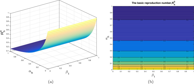
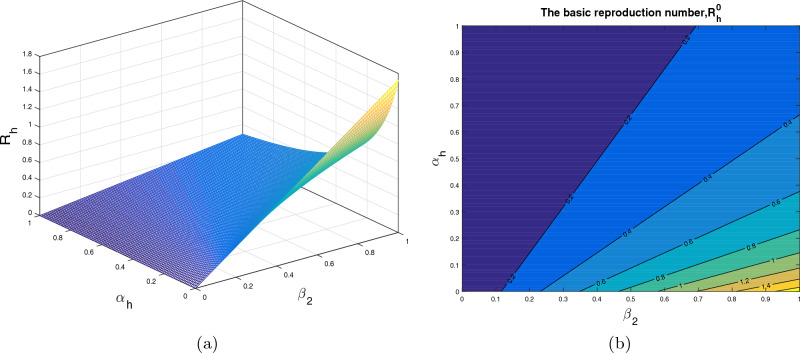
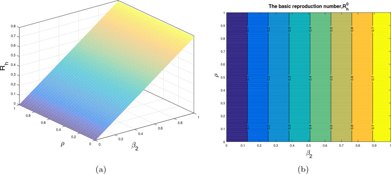
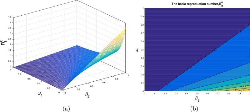
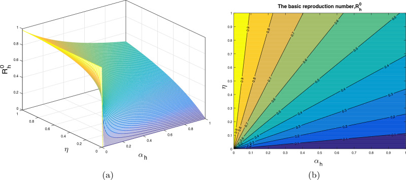
In this section, we analyze the impact of some model parameters on ${\mathcal{R}}_0$. The basic reproduction number ${\mathcal{R}}_0$ is a key biological parameter that plays an important role in describing the disease dynamics and its possible control. In these graphical results, we consider the disease transmission rates ${\beta }_1$, ${\beta }_2$, vaccination rate ${\alpha }_h$, recovery rates $\rho ,$ ${\omega }_1$ and vaccine waning rate $\eta$. The respective graphical results are shown in Figs. 2a, 3, 4, 5 and 6a, while the corresponding contour plots in each case are shown in Figs. 2b, 3, 4, 5 and 6b. Figure 2 shows the combine impact of ${\beta }_1$ and ${\alpha }_h$ on ${\mathcal{R}}_0$. It shows that the ${\mathcal{R}}_0$ decreases with a decrease in transmission coefficient ${\beta }_1$ and an increase in vaccination rate ${\alpha }_h$. Further, impact of ${\beta }_2$ along with ${\alpha }_h$ upon ${\mathcal{R}}_0$ is demonstrated in the Fig. 3a with the corresponding counter plot 3b. It can be observed that with the increase in vaccination rate and reduction in contact rate $\beta$ the basic reproduction reduces to a value less than 1. Similarly, the impact of $\rho$ and ${\beta }_2$, ${\omega }_1$ and ${\beta }_2$, $\eta$ and ${\alpha }_h$ are presented in Figs. 4a, 5a, and 6a respectively. We can observe that with the decrease in disease transmission rate ${\beta }_2$ and enhancement in vaccination rate ${\alpha }_h$ and recovery rate $\omega$ the basic reproduction decreases significantly to a value less than unity.

Figure 2.

The subplot (a) illustrate the impact of ${\beta }_1$ (disease transmission coefficient relative to $I_h$) and ${\alpha }_h$ (vaccination rate ) on ${\mathcal{R}}_0$, where (b) shows the respective contour plot.

Figure 3.

The subplot (a) analyze the impact of ${\beta }_2$ (disease transmission coefficient relative to $I_r$) and ${\alpha }_h$ (vaccination rate ) on ${\mathcal{R}}_0$, where (b) shows the respective contour plot.

Figure 4.

The subplot (a) demonstrate the impact of ${\beta }_2$ (disease transmission coefficient relative to $I_r$) and $\rho$ (recovery rate of $C_h$) on ${\mathcal{R}}_0$, where (b) shows the respective contour plot.

Figure 5.

The subplot (a) demonstrate the impact of ${\beta }_2$ (disease transmission coefficient relative to $I_r$) and ${\omega }_1$ (recovery rate of $I_h$) on ${\mathcal{R}}_0$, where (b) shows the respective contour plot.

Figure 6.

The subplot (a) demonstrate the impact of ${\alpha }_h$ (vaccination rate) and $\eta$ (loss of immunity rate) on ${\mathcal{R}}_0$, where (b) shows the respective contour plot.

Numerical results of the fractional model

In this section, we first investigate the numerical solution of the Caputo fractional monkeypox model. The generalized fractional Adams-Bash forth-Moulton approach³⁴, an effective iterative method is used to solve the model numerically. The simulation for different model parameters and different values of $\vartheta$ are carried out using the generated numerical technique and the values for model parameters are listed in Table 1. The subsequent subsection contains the iterative solution.

Numerical technique

A concise numerical method for the approximate solution of the monkeypox transmission model in the Caputo sense is shown in this subsection. For this purpose, the fractional Adams-Bashforth-Moulton is used. The system (6) can be recomposed in the subsequent problem to get the desired scheme:

$$\begin{array}{c}\hfill \left\{\begin{array}{c}{}^C{D}_t^{\vartheta }\mathbf{v}(t)=\mathcal{M}(t,\mathbf{v}(t)),0<t<\mathcal{T},\hfill \\ {\mathbf{v}}^{(m)}(0)={\mathbf{v}}_0^{(m)},m=0,1,\dots ,v,v=[\vartheta ],\hfill \end{array}\right)\end{array}$$ 22

where, $\mathbf{v}=(S_h,E_h,I_h,C_h,V_h,R_h,S_r,E_r,I_r,R_r)\in {\mathbb{R}}_{+}^{10}$, and $\mathcal{M}(t,\mathbf{v}(t))$ shows a continuous real valued function. Using the concept of integral in Caputo case, the aforementioned Eq. (22) is considered as follows:

$$\begin{array}{c}\hfill \mathbf{v}(t)=\sum _{\mathtt{m}=0}^{v-1}{\mathbf{v}}_0^{(m)}\frac{t^m}{m!}+\frac{1}{\mathrm{\Gamma }(\vartheta )}{\int }_0^t{(t-x)}^{\vartheta -1}\mathcal{M}(x,\mathbf{v}(x))dx.\end{array}$$ 23

In order to use the procedure in³⁴, a uniform grid on $[0,\mathcal{T}]$ with step size $h=\frac{\mathcal{T}}{N}$, $N\in \mathbb{N}$, where $t_u=uh,u=0,1\dots ,N$ is considered. Thus, the proposed model in (6) can be treated as:

$$\begin{array}{cc}\hfill S_{h_{u+1}}(t)=& S_{h_0}+\frac{h^{\vartheta }}{\mathrm{\Gamma }\left(\vartheta ,+,2\right)}\{{\mathrm{\Phi }}_h-\left({\alpha }_1,I_h^m,+,{\alpha }_2,I_r^m\right)\frac{S_h^m}{N_h^m}-{\mathtt{k}}_1{S}_h^m+\eta V_h^m\}+\hfill \\ \hfill \\ \hfill & \frac{h^{\vartheta }}{\mathrm{\Gamma }(\vartheta +2)}\sum _{k=0}^u{b}_{k,u+1}\{{\mathrm{\Phi }}_h-\left({\alpha }_1,I_{h_k},+,{\alpha }_2,I_{r_k}\right)\frac{S_{h_k}}{N_{h_k}}-{\mathtt{k}}_1{S}_{h_k}+\eta V_{h_k}\},\hfill \\ \hfill \\ \hfill E_{h_{u+1}}(t)=& E_{h_0}+\frac{h^{\vartheta }}{\mathrm{\Gamma }(\vartheta +2)}\{({\alpha }_1{I}_h^m+{\alpha }_2{I}_r^m)\frac{S_h^m}{N_h^m}+{\mathtt{k}}_2{E}_h^m\}+\frac{h^{\vartheta }}{\mathrm{\Gamma }(\vartheta +2)}\hfill \\ \hfill \\ \hfill & \sum _{j=0}^u{b}_{k,u+1}\{({\alpha }_1{I}_{h_k}+{\alpha }_2{I}_{r_k})\frac{S_{h_k}}{N_{h_k}}+{\mathtt{k}}_2{E}_{h_k}\},\hfill \\ \hfill \\ \hfill I_{h_{u+1}}(t)=& I_{h_0}+\frac{h^{\vartheta }}{\mathrm{\Gamma }(\vartheta +2)}\{\beta E_h^m-{\mathtt{k}}_3{I}_h^m\}+\frac{h^{\vartheta }}{\mathrm{\Gamma }(\vartheta +2)}\sum _{k=0}^u{b}_{k,u+1}\{E_{h_k}-{\mathtt{k}}_3{I}_{h_k}\},\hfill \\ \hfill \\ \hfill C_{h_{u+1}}(t)=& C_{h_0}+\frac{h^{\vartheta }}{\mathrm{\Gamma }(\vartheta +2)}\{\gamma I_h^m-{\mathtt{k}}_4{C}_h^m\}+\frac{h^{\vartheta }}{\mathrm{\Gamma }(\vartheta +2)}\sum _{k=0}^u{b}_{k,u+1}\{\gamma I_{h_k}-{\mathtt{k}}_4{C}_{h_k}\},\hfill \\ \hfill \\ \hfill V_{h_{u+1}}(t)=& V_{h_0}+\frac{h^{\vartheta }}{\mathrm{\Gamma }(\vartheta +2)}\{{\alpha }_h{S}_h^m-{\mathtt{k}}_5{V}_h^m\}+\frac{h^{\vartheta }}{\mathrm{\Gamma }(\vartheta +2)}\sum _{k=0}^u{b}_{k,u+1}\{{\alpha }_h{S}_{h_k}-{\mathtt{k}}_5{V}_{h_k}\},\hfill \\ \hfill \\ \hfill R_{h_{k+1}}(t)=& R_{h_0}+\frac{h^{\vartheta }}{\mathrm{\Gamma }\left(\vartheta ,+,2\right)}\{\rho C_h^m+{\omega }_1{I}_h^m-{\mu }_h{R}_h^m\}+\frac{h^{\vartheta }}{\mathrm{\Gamma }(\vartheta +2)}\sum _{k=0}^u{b}_{k,u+1}\{\rho C_{h_k}+{\omega }_1{I}_{h_k}-{\mu }_h{R}_{h_k}\},\hfill \\ \hfill \\ \hfill textsectio{n}_{r_{u+1}}(t)=& S_{r_0}+\frac{h^{\vartheta }}{\mathrm{\Gamma }(\vartheta +2)}\{{\varphi }_r-\frac{{\beta }_3{I}_r^m}{N_r^m}{S}_r^m-{\mu }_r{S}_r^m\}+\frac{h^{\vartheta }}{\mathrm{\Gamma }(\vartheta +2)}\sum _{k=0}^u{b}_{k,u+1}\{{\varphi }_r-\frac{{\beta }_3{I}_{r_k}}{N_{r_k}}{S}_{r_k}-{\mu }_r{S}_{r_k}\},\hfill \\ \hfill \\ \hfill E_{r_{u+1}}(t)=& E_{r_0}+\frac{h^{\vartheta }}{\mathrm{\Gamma }(\vartheta +2)}\{\frac{{\beta }_3{I}_r^m}{N_r^m}{S}_r^m-{\mathtt{k}}_6{E}_r^m\}+\frac{h^{\vartheta }}{\mathrm{\Gamma }(\vartheta +2)}\sum _{k=0}^u{b}_{k,u+1}\{\frac{{\beta }_3{I}_{r_k}}{N_{r_k}}{S}_{r_k}-{\mathtt{k}}_6{E}_{r_k}\},\hfill \\ \hfill \\ \hfill I_{r_{u+1}}(t)=& I_{r_0}+\frac{h^{\vartheta }}{\mathrm{\Gamma }(\vartheta +2)}\{ϵE_r^m-{\mathtt{k}}_7{I}_r^m\}+\frac{h^{\vartheta }}{\mathrm{\Gamma }(\vartheta +2)}\sum _{k=0}^u{b}_{k,u+1}\{ϵE_{r_j}-{\mathtt{k}}_7{I}_{r_j}\},\hfill \\ \hfill \\ \hfill R_{r_{k+1}}(t)=& R_{r_0}+\frac{h^{\vartheta }}{\mathrm{\Gamma }(\vartheta +2)}\{{\omega }_2{I}_r^m-{\mu }_r{R}_r^m\}+\frac{h^{\vartheta }}{\mathrm{\Gamma }(\vartheta +2)}\sum _{k=0}^u{b}_{i,u+1}\{{\omega }_2{I}_{r_k}-{\mu }_r{R}_{r_k}\},\hfill \end{array}$$

where,

$$\begin{array}{cc}\hfill S_{h_{u+1}}^m(t)=& S_{h_0}+\frac{1}{\mathrm{\Gamma }(\vartheta )}\sum _{k=0}^u{\theta }_{k,u+1}\{{\mathrm{\Phi }}_h-\left({\alpha }_1,I_{h_k},+,{\alpha }_2,I_{r_k}\right)\frac{S_{h_k}}{N_{h_k}}-{\mathtt{k}}_1{S}_{h_k}+\eta V_{h_k}\},\hfill \\ \hfill \\ \hfill E_{h_{u+1}}^m(t)=& E_{h_0}+\frac{1}{\mathrm{\Gamma }(\vartheta )}\sum _{k=0}^u{\theta }_{k,u+1}\{\left({\alpha }_1,I_{h_k},+,{\alpha }_2,I_{r_k}\right)\frac{S_{h_k}}{N_{h_k}}-{\mathtt{k}}_2{E}_{h_k}\},\hfill \\ \hfill \\ \hfill I_{h_{u+1}}^m(t)=& I_{h_0}+\frac{1}{\mathrm{\Gamma }(\vartheta )}\sum _{k=0}^u{\theta }_{k,u+1}\{\beta E_{h_k}-{\mathtt{k}}_3{I}_{h_k}\},\hfill \\ \hfill \\ \hfill C_{h_{u+1}}^m(t)=& C_{h_0}+\frac{1}{\mathrm{\Gamma }(\vartheta )}\sum _{k=0}^u{\theta }_{k,u+1}\{\rho C_{h_k}+{\omega }_1{I}_{h_k}-{\mu }_h{R}_{h_k}\},\hfill \\ \hfill \\ \hfill V_{h_{u+1}}^m(t)=& V_{h_0}+\frac{1}{\mathrm{\Gamma }(\vartheta )}\sum _{k=0}^u{\theta }_{k,u+1}\{{\alpha }_h{S}_{h_k}-{\mathtt{k}}_5{V}_{h_k}\},\hfill \\ \hfill \\ \hfill R_{h_{u+1}}^m(t)=& R_{h_0}+\frac{1}{\mathrm{\Gamma }(\vartheta )}\sum _{k=0}^u{\theta }_{k,u+1}\{\rho C_{h_k}+{\omega }_1{I}_{h_k}-{\mu }_h{R}_{h_k}\},\hfill \\ \hfill \\ \hfill textsectio{n}_{r_{u+1}}^m(t)=& S_{r_0}+\frac{1}{\mathrm{\Gamma }(\vartheta )}\sum _{k=0}^u{\theta }_{k,u+1}\{{\varphi }_r-\frac{{\beta }_3{I}_{r_k}}{N_{r_k}}{S}_{r_k}-{\mu }_r{S}_{r_k}\},\hfill \\ \hfill \\ \hfill E_{r_{u+1}}^m(t)=& E_{r_0}+\frac{1}{\mathrm{\Gamma }(\vartheta )}\sum _{k=0}^u{\theta }_{k,u+1}\{\frac{{\beta }_3{I}_{r_k}}{N_{r_k}}{S}_{r_k}-{\mathtt{k}}_6{E}_{r_k}\},\hfill \\ \hfill \\ \hfill I_{r_{k+1}}^m(t)=& I_{r_0}+\frac{1}{\mathrm{\Gamma }(\vartheta )}\sum _{k=0}^u{\theta }_{k,u+1}\{ϵE_{r_k}-{\mathtt{k}}_7{I}_{r_k}\},\hfill \\ \hfill \\ \hfill R_{r_{u+1}}^m(t)=& R_{r_0}+\frac{1}{\mathrm{\Gamma }(\vartheta )}\sum _{k=0}^u{\theta }_{k,u+1}\{{\omega }_2{I}_{r_k}-{\mu }_r{R}_{r_k}\},\hfill \\ \hfill \\ \hfill \end{array}$$

Further, we have in the above expressions

$$\begin{array}{c}\hfill b_{k,u+1}=\left\{\begin{array}{c}{u}^{\vartheta +1}-(u-\vartheta ){(u+1)}^{\vartheta },k=0\hfill \\ {(u-k+2)}^{\vartheta +1}+{(u-k)}^{\vartheta +1}-2{(u-k+1)}^{\vartheta +1},1\le k\le u,\hfill \\ 1,k=u+1,\hfill \end{array}\right)\end{array}$$

and

$$\begin{array}{c}\hfill {\theta }_{k,u+1}=\frac{h^{\vartheta }}{\vartheta }\left[{(u-k+1)}^{\vartheta },+,{(u-k)}^{\vartheta }\right],0\le k\le u.\end{array}$$

Simulation of the fractional monkeypox model

In this section, we applied the iterative technique developed in the preceding section in order to simulate the monkeypox Caputo epidemic model (6). The simulation results are illustrated by taking the baseline values of estimated parameters listed in Table 1. In the simulation results, we mainly focus on the dynamics of infected human and animal populations. Initially, in the simulation, we analyze the dynamics of model state variables for various values of $\vartheta \in (0,1]$ to study the impact of memory index on disease incidence. Further, the influence of variation in the recovery rate ${\omega }_1$ on the behavior of the infected human population is predicted for many values of fractional order $\vartheta$. Moreover, we considered different scenarios by decreasing the effective contact rates among susceptible humans and infected animals (i.e., ${\beta }_1,{\beta }_2$) and the parameter ${\beta }_3$ showing the effective contact rate between susceptible and infected animals. In addition, these simulations are performed for various non-integer values of the parameter $\vartheta$. The detailed discussion of the aforementioned simulation is described in the following subparts.

Impact of memory index ($\vartheta$)

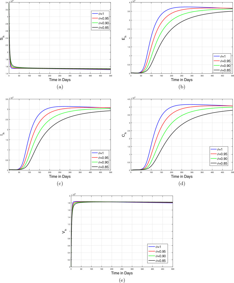
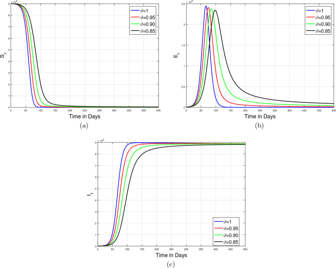
In the first case of simulation, we illustrate the impact of only fractional order $\vartheta$ of the Caputo operator on the model dynamics. The graphical results are shown in Figs. 7a–e and 8a–c. The dynamics of only human population classes are shown in Fig. 7 while Fig. 8 illustrates the dynamical aspects of only animal subpopulation. The simulation in both cases is performed for four values of $\vartheta =1,0.95,0.90,0.85$. The time length considered in the simulation is taken to 500 days. It is observed that under the specific conditions, the solution trajectories in both population classes are converged to the steady state for all values of fractional order $\vartheta$.

Figure 7.

Simulations of only human classes in fractional monkeypox epidemic model (6) for various values of fractional order $\vartheta$.

Figure 8.

Simulations of only non-human classes in fractional monkeypox epidemic model (6) for various values of fractional order $\vartheta$.

Impact of recovery rate ${\omega }_1$ and memory index ($\vartheta$)

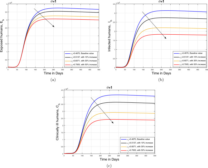
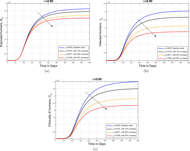
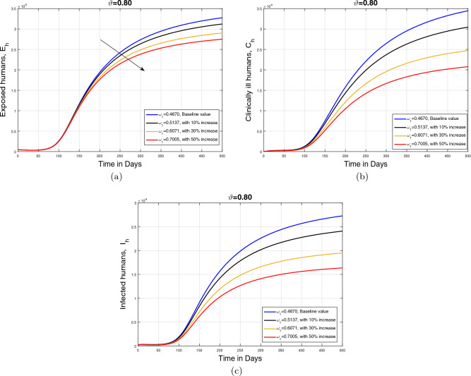
In this subpart, we analyzed the impact of variation in recovery rate ${\omega }_1$ on the dynamics of cumulative cases of exposed $E_h$, infected $I_h$, and clinically infected $C_h$ human under different values of memory index ($\vartheta$). The parameter showing recovery rate is perturbed with different rates (with baseline and with $10\%$, $30\%$, and $50\%$ increase) depending on the treatment strength provided to the infected human population. The resulting simulation is accomplished in Figs. 9, 10 and 11 with subplots (a–c) for three values of fractional order $\vartheta$. It is observed that with an increase in parameter ${\omega }_1$, the infected population in all aforementioned classes reduces showing the impact of treatment on the disease incidence. Additionally, it can observed that in the case of smaller values of $\vartheta$, the decline in the infected population is slightly faster.

Figure 9.

Impact of recovery rate ${\omega }_1$ with $\vartheta =1$.

Figure 10.

Impact of recovery rate ${\omega }_1$ with $\vartheta =0.90$.

Figure 11.

Impact of recovery rate ${\omega }_1$ with $\vartheta =0.80$.

Impact of disease transmission rates and memory index ($\vartheta$)

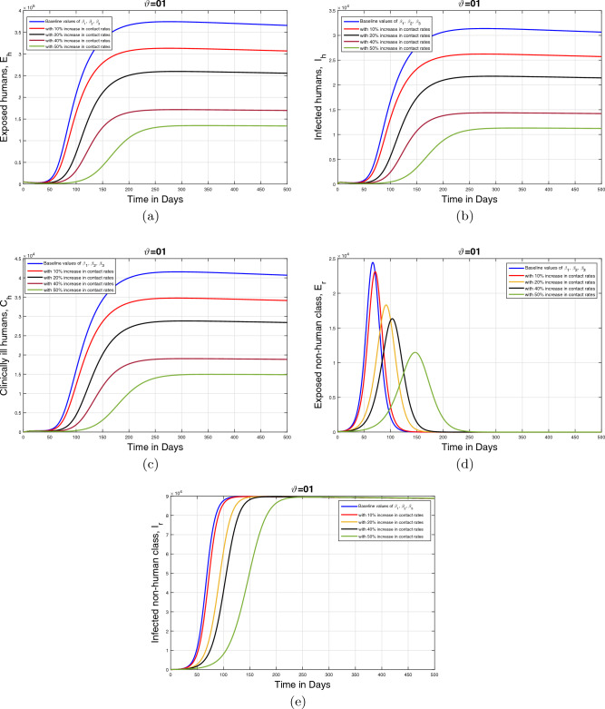
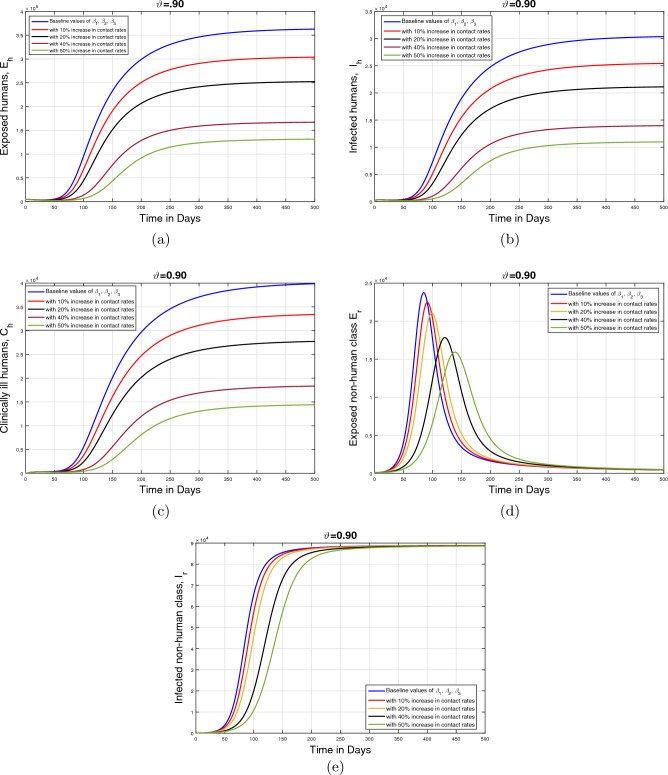
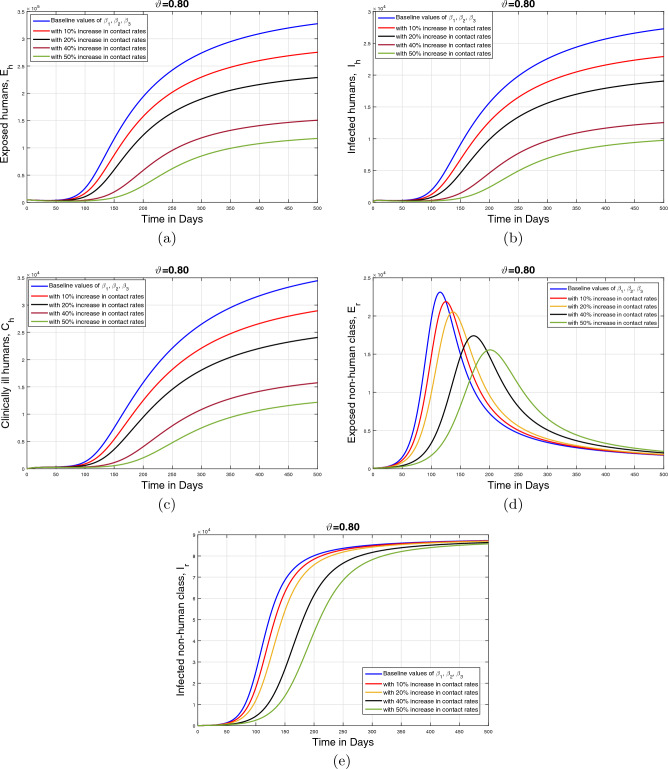
This section describes the influence of the infection transmission rates ${\beta }_1,{\beta }_2$, and ${\beta }_3$ on the dynamics of infected human and animal population classes. The graphical results are initially performed for the baseline values of the aforementioned parameters given in Table 1. Subsequently, the parameter values are decreased with $10\%,$ $20\%,$ $40\%$, and $50\%$ to the estimated values. Furthermore, the simulation results are presented for three values of fractional order $\vartheta$. These resulting simulations for the human population are shown in Figs. 12, 13 and 14 with respective subplots from (a–c) while the dynamics of the infected animal population are demonstrated in Figs. 12, 13 and 14d, e. In all plots, it is evident that the cumulative infected population significantly decreases as the infection transmission rates are reduced. Moreover, it can be seen from Figs. 13 and 14, that fractional values of $\vartheta$ provide more insights enhancing our understanding of the disease dynamics. disease dynamics. Consequently, these graphical interpretations suggest that the effective control of the monkeypox disease and the reduction of disease-induced mortality can be achieved by implementing appropriate treatment and disinfection techniques.

Figure 12.

Impact of contact rates ${\beta }_1,{\beta }_2,{\beta }_3$ with different rated and $\vartheta =1$.

Figure 13.

Impact of contact rates${\beta }_1,{\beta }_2,{\beta }_3$ with different rated and $\vartheta =0.90$.

Figure 14.

Impact of contact rates ${\beta }_1,{\beta }_2,{\beta }_3$ with different rated and $\vartheta =0.80$.

Conclusion

In this manuscript, we analyzed the dynamics of a novel monkeypox infection with the case study of the recently reported outbreak. The model is first formulated using an integer-order nonlinear system of ten differential equations. The human population was divided into six distinct subgroups, while the animal population was divided into four classes. To estimate the model parameters, we fit the model to the actual cases of the 2022 monkeypox outbreak in the USA. Moreover, keeping the importance of the fractional modeling approach, the integer case model is extended to fractional order via the well-known Caputo operator. In the initial stage, we presented a comprehensive theoretical analysis of the fractional monkeypox model, including the existence and uniqueness of the solutions. The existence and stability analysis of the model equilibria are provided. Furthermore, the fractional model is solved numerically using the fractional Adams-Bashforth-Moulton approach. The simulation results illustrate the impact of disease incidence graphically, considering both the baseline values of the parameters and different values of the fractional order of the Caputo operator. Moreover, the model is simulated by increasing the parameter ${\omega }_1$ (the recovery rate) and decreasing the disease transmission coefficients ${\beta }_1,{\beta }_2,{\beta }_3$ with different rates to their baseline values. The implementation of a real-data set of monkeypox infections makes this study more visible and important within the existing literature.

Author contributions

B.L. and M.A. improve the language of the manuscript, reviewing and editing, validate governing equations and all mathematical results with care, and project admiration. S.F and S.U. wrote the original manuscript, performed mathematical results and numerical simulations. R.N. and S.W.T. conceptualized the main problem, supervision, formal analysis, and perform data analysis. All authors are agreed on the final draft of the submission file.

Data availability

The data that support the findings of this study are available from the corresponding author up on reasonable request. Further, no experiments on humans and/or the use of human tissue samples involved in this study.

Competing interest

The authors declare no competing interests.

References

- 1.Centers for Disease Control and Prevention 2021 National Center for Emerging and Zoonotic Infectious Diseases (NCEZID), Division of High-Consequence Pathogens and Pathology (DHCPP), Monkeypox (2021, accessed 10 Nov 2021). https://www.cdc.gov/poxvirus/Monkeypox/index.html.
- 2.Jezek Z, Szczeniowski M, Paluku KM, Mutombo M, Grab B. Human monkeypox: Confusion with chickenpox. Acta Trop. 1988;45(4):297–307. [PubMed] [Google Scholar]
- 3.CDC. What you should know about Monkeypox (2003). https://www.cdc.gov/poxvirus/monkeypox/.
- 4.Bunge EM, Hoet B, Chen L, Lienert F, Weidenthaler H, Baer LR, Steffen R. The changing epidemiology of human monkeypox? A potential threat? A systematic review. PLoS Negl. Trop. Dis. 2022;16(2):e0010141. doi: 10.1371/journal.pntd.0010141. [DOI] [PMC free article] [PubMed] [Google Scholar]
- 5.Durski KN, McCollum AM, Nakazawa Y, Petersen BW, Reynolds MG, Briand S, Djingarey MH, Olson V, Damon IK, Khalakdina A. Emergence of monkeypox? West and central Africa. Morb. Mortal. Wkly. Rep. 2018;67(10):306. doi: 10.15585/mmwr.mm6710a5. [DOI] [PMC free article] [PubMed] [Google Scholar]
- 6.2021 Nigeria Centre for Disease Control, Monkeypox outbreak situation report (2021, accessed 10 Nov 2021). https://ncdc.gov.ng/report/.
- 7.Centers for Disease Control and Prevention, National Center for Emerging and Zoonotic Infectious Diseases(NCEZID), Division of High-Consequence Pathogens and Pathology (DHCPP), Monkeypox (2021, accessed 11 Nov 2021). https://cdc.gov/poxvirus/monkeypox/index.html.
- 8.Peter OJ, Kumar S, Kumari N, Oguntolu FA, Oshinubi K, Musa R. Transmission dynamics of Monkeypox virus: A mathematical modelling approach. Model. Earth Syst. Env. 2022;8(3):3423–3434. doi: 10.1007/s40808-021-01313-2. [DOI] [PMC free article] [PubMed] [Google Scholar]
- 9.Ngungu M, Addai E, Adeniji A, Adam UM, Oshinubi K. Mathematical epidemiological modeling and analysis of monkeypox dynamism with non-pharmaceutical intervention using real data from United Kingdom. Front. Public Health. 2023;11:1101436. doi: 10.3389/fpubh.2023.1101436. [DOI] [PMC free article] [PubMed] [Google Scholar]
- 10.Baba BA, Bilgehan B. Optimal control of a fractional order model for the COVID-19 pandemic. Chaos Solit. Fract. 2021;144:110678. doi: 10.1016/j.chaos.2021.110678. [DOI] [PMC free article] [PubMed] [Google Scholar]
- 11.Ameen I, Baleanu D, Ali HM. An efficient algorithm for solving the fractional optimal control of SIRV epidemic model with a combination of vaccination and treatment. Chaos Solit. Fract. 2020;137:109892. doi: 10.1016/j.chaos.2020.109892. [DOI] [Google Scholar]
- 12.Abioye AI, Peter OJ, Ogunseye HA, Oguntolu FA, Oshinubi K, Ibrahim AA, Khan I. Mathematical model of COVID-19 in Nigeria with optimal control. Results Phys. 2021;28:104598. doi: 10.1016/j.rinp.2021.104598. [DOI] [PMC free article] [PubMed] [Google Scholar]
- 13.Kumar S, Chauhan RP, Momani S, Hadid S. Numerical investigations on COVID-19 model through singular and non-singular fractional operators. Numer. Methods Part. Differ. Equ. 2020;2020:896. [Google Scholar]
- 14.Bankuru SV, Kossol S, Hou W, Mahmoudi P, Rychta J, Taylor D. A game-theoretic model of Monkeypox to assess vaccination strategies. PeerJ. 2020;8:e9272. doi: 10.7717/peerj.9272. [DOI] [PMC free article] [PubMed] [Google Scholar]
- 15.Usman S, Adamu II. Modeling the transmission dynamics of the monkeypox virus infection with treatment and vaccination interventions. J. Appl. Math. Phys. 2017;5(12):2335. doi: 10.4236/jamp.2017.512191. [DOI] [Google Scholar]
- 16.Alshehri A, Ullah S. Optimal control analysis of Monkeypox disease with the impact of environmental transmission. AIMS Math. 2023;8(7):16926–16960. doi: 10.3934/math.2023865. [DOI] [Google Scholar]
- 17.Allehiany FM, Darassi MH, Ahmad I, Khan MA, Tag-Eldin EM. Mathematical modeling and backward bifurcation in monkeypox disease under real observed data. Results Phys. 2023;2023:106557. doi: 10.1016/j.rinp.2023.106557. [DOI] [PMC free article] [PubMed] [Google Scholar]
- 18.Rihan, F. A., Baleanu, D., Lakshmanan, S. & Rakkiyappan, R. On fractional SIRC model with salmonella bacterial infection. In Abstract and Applied Analysis Vol. 2014 (2014).
- 19.Baba IA, Nasidi BA. Fractional order epidemic model for the dynamics of novel COVID-19. Alexandr. Eng. J. 2021;60(1):537–548. doi: 10.1016/j.aej.2020.09.029. [DOI] [Google Scholar]
- 20.Rihan, F. A. Numerical modeling of fractional-order biological systems. In Abstract and Applied Analysis Vol. 2013 (2023).
- 21.Ali A, Ullah S, Khan MA. The impact of vaccination on the modeling of COVID-19 dynamics: A fractional order model. Nonlinear Dyn. 2022;110:3921–3940. doi: 10.1007/s11071-022-07798-5. [DOI] [PMC free article] [PubMed] [Google Scholar]
- 22.Saeedian M, Khalighi M, Azimi-Tafreshi N, Jafari GR, Ausloos M. Memory effects on epidemic evolution: The susceptible-infected-recovered epidemic model. Phys. Rev. E. 2017;95(2):022409. doi: 10.1103/PhysRevE.95.022409. [DOI] [PMC free article] [PubMed] [Google Scholar]
- 23.Ahmed I, Baba IA, Yusuf A, Kumam P, Kumam W. Analysis of Caputo fractional-order model for COVID-19 with lockdown. Adv. Differ. Equ. 2020;2020(1):394. doi: 10.1186/s13662-020-02853-0. [DOI] [PMC free article] [PubMed] [Google Scholar]
- 24.Aba-Oud MA, Ali A, Alrabaiah H, Ullah S, Khan MA, Islam S. A fractional order mathematical model for COVID-19 dynamics with quarantine, isolation, and environmental viral load. Adv. Differ. Equ. 2021;1:1–19. doi: 10.1186/s13662-021-03265-4. [DOI] [PMC free article] [PubMed] [Google Scholar]
- 25.Baba IA, Sani MA, Nasidi BA. Fractional dynamical model to assess the efficacy of facemask to the community transmission of COVID-19. Comput. Methods Biomech. Biomed. Eng. 2022;25(14):1588–98. doi: 10.1080/10255842.2021.2024170. [DOI] [PubMed] [Google Scholar]
- 26.Ali A, Alshammari FS, Islam S, Khan MA, Ullah S. Modeling and analysis of the dynamics of novel coronavirus (COVID-19) with Caputo fractional derivative. Results Phys. 2021;20:103669. doi: 10.1016/j.rinp.2020.103669. [DOI] [PMC free article] [PubMed] [Google Scholar]
- 27.Khan MA, Ullah S, Kumar S. A robust study on 2019-nCOV outbreaks through non-singular derivative Eur. Phys. J. Plus. 2021;136:1–20. doi: 10.1140/epjp/s13360-021-01159-8. [DOI] [PMC free article] [PubMed] [Google Scholar]
- 28.Khan A, Sabbar Y, Din A. Stochastic modeling of the Monkeypox 2022 epidemic with cross-infection hypothesis in a highly disturbed environment. Math. Biosci. Eng. 2022;19(12):13560–13581. doi: 10.3934/mbe.2022633. [DOI] [PubMed] [Google Scholar]
- 29.Alzubaidi AM, Othman HA, Ullah S, Ahmad N, Alam MM. Analysis of Monkeypox viral infection with human to animal transmission via a fractional and Fractal-fractional operators with power law kernel. Math. Biosci. Eng. 2023;20(4):6666–6690. doi: 10.3934/mbe.2023287. [DOI] [PubMed] [Google Scholar]
- 30.Milici C, Draganescu G, Machado JT. Introduction to Fractional Differential Equations. Springer; 2018. [Google Scholar]
- 31.Podlubny I. Fractional Differential Equations: An Introduction to Fractional Derivatives, Fractional Differential Equations, to Methods of Their Solution and Some of Their Applications. Elsevier; 1998. [Google Scholar]
- 32.USA population (2022, accessed Nov 2022). https://www.worldometers.info/world-population/us-population/.
- 33.Van den Driessche P, Watmough J. Reproduction numbers and sub-threshold endemic equilibria for compartmental models of disease transmission. Math. Biosci. 2002;180(1–2):29–48. doi: 10.1016/S0025-5564(02)00108-6. [DOI] [PubMed] [Google Scholar]
- 34.Baskonus HM, Bulut H. On the numerical solutions of some fractional ordinary differential equations by fractional Adams-Bashforth-Moulton method. Open Math. 2015;13:1. doi: 10.1515/math-2015-0052. [DOI] [Google Scholar]
Associated Data
This section collects any data citations, data availability statements, or supplementary materials included in this article.
Data Availability Statement