Analysis of polar primary metabolites in biological samples using targeted metabolomics and LC-MS

Summary

Primary metabolites are molecules of essential biochemical reactions that define the biological phenotype. All primary metabolites cannot be measured in a single analysis. In this protocol, we outline the multiplexed and quantitative measurement of 106 metabolites that cover the central part of primary metabolism. The protocol includes several sample preparation techniques and one liquid chromatography-mass spectrometry method. Then, we describe the steps of the bioinformatic data analysis to better understand the metabolic perturbations that may occur in a biological system.

For complete details on the use and execution of this protocol, please refer to: Costanza et al.,¹ Blomme et al.,² Blomme et al.,³ Guillon et al.,⁴ Stuani et al.⁵

Graphical abstract

Highlights

• •Isolating and purifying polar metabolites from biological samples
• •Preparing the LC-MS system, MRM transitions, QC evaluation, and injecting the samples
• •Basic LC-MS data analysis, peak interpretation, and quantitative evaluation
• •Basic bioinformatic data analysis using R and generation of essential plots

Publisher’s note: Undertaking any experimental protocol requires adherence to local institutional guidelines for laboratory safety and ethics.

Primary metabolites are molecules of essential biochemical reactions that define the biological phenotype. All primary metabolites cannot be measured in a single analysis. In this protocol, we outline the multiplexed and quantitative measurement of 106 metabolites that cover the central part of primary metabolism. The protocol includes several sample preparation techniques and one liquid chromatography-mass spectrometry method. Then, we describe the steps of the bioinformatic data analysis to better understand the metabolic perturbations that may occur in a biological system.

Before you begin

The present liquid chromatography-mass spectrometry (LC-MS) protocol allows the targeted identification and quantification of 106 molecules using the multiple-reaction monitoring (MRM) acquisition mode (detailed parameters for each compound are provided in Table S1). In this mode, MS isolates a pre-defined molecule according to its nominal mass, fragments this molecule in multiple fragments, and then gives their respective masses. The combination of the nominal mass of the whole molecule and its fragments is called transition and this value is molecule-specific. Here, we use multiple transitions for each molecule and chromatographic retention time to unambiguously detect the metabolites of interest. The protocol outlined below is divided in three parts: i) sample preparation, ii) metabolite purification, and iii) LC-MS analysis. At the end of each part, the protocol can be paused by freezing the samples at −20°C (short term storage; up-to a week) or −80°C (long term storage; up-to a year). We provide three variants of the metabolite purification protocol, in function of the starting material complexity. The MS analysis, described in the last part of the protocol, is a common step that is adapted for all samples and purification techniques.

Note: The present protocol is compatible with the Poly Unsaturated Fatty Acids (PUFA) analysis method described elsewhere (see Turtoi E et al.⁶). If the same sample is processed with both methods, we recommend to start with the PUFA isolation protocol, but adding to the sample the internal standard described below (“Sample Preparation” step). Continue PUFA isolation until the “PUFA purification using Solid Phase Extraction (SPE) columns” chapter, step 13c. Importantly, do not discard, but store the flow-through/filtrate sample obtained at step 13c. Evaporate the sample and resuspend it in water (generally 1 mL). Proceed with the LC-MS analysis, as described in the “LC-MS Analysis” chapter of the present method. Note that due to the higher amount of starting material in the PUFA method, such samples need to be more diluted than the samples obtained with the present method, intended only for general metabolite analysis.

• 1.Consider how the sample will be prepared.

Tissue and cell samples can be homogenized using different methods. For cells and soft tissues (e.g., cultured cells and liver samples), bead-based homogenization using, for instance, the Precellys 24 homogenizer (see key resources table below) is sufficient. For harder tissues (e.g., bone), mortar and pestle combined with snap-freezing are more appropriate. Note that during homogenization, the sample should be kept or rapidly transferred into the crushing solution (generally containing up to 80% of an organic solvent, such as methanol). If homogenization is performed with beads and agitating equipment (e.g., Precellys 24), the sample can easily leak unless 1.5 mL tubes with screw-caps and rubber O-rings (such as the ones referenced here) are used. Homogenization of soft tissue/cells can be performed also with TissueRuptor II (Qiagen) and disposable probes or Ultra-Turrax (Ika).

• 2.Familiarize yourself with the chemicals used.

CRITICAL: Be very careful when handling the hazardous chemicals required for this protocol. Specifically, solvents (methanol, acetonitrile, chloroform, acetone, and isopropanol), formic acid, and sodium dodecyl sulfate (SDS) are used under a fume hood and wearing personal protective equipment (gloves, goggles and laboratory coat). The list below summarizes some Hazard (H) and Precautionary (P) statements concerning these chemicals:

Hazard

H225: Highly flammable liquid and vapor (methanol, acetonitrile, isopropanol, acetone).

H226: Flammable liquid and vapor (formic acid).

H228: Flammable solid (SDS).

H290: May be corrosive to metals (formic acid).

H301 + H311 + H331: Toxic if swallowed, in contact with skin, or inhaled (methanol, formic acid).

H302 + H332: Harmful if swallowed or inhaled (all).

H314: Causes severe skin burns and eye damage (formic acid).

H315: Causes skin irritation (SDS, chloroform).

H318: Causes serious eye damage (SDS).

H319: Causes serious eye irritation (acetonitrile, isopropanol, acetone).

H335: May cause respiratory irritation (SDS).

H336: May cause drowsiness or dizziness (chloroform, isopropanol, acetone).

H370: Causes damage to organs (eyes, central nervous system) (methanol).

H372: Causes damage to organs (liver, kidney) in case of prolonged or repeated exposure (chloroform).

H412: Harmful to aquatic life with long-lasting effects (SDS, methanol, chloroform).

Precaution

P201: Obtain special instructions before use (chloroform).

P210: Keep away from heat, sparks, open flames, hot surfaces. No smoking (all).

P223: Keep container tightly closed (all).

P261: Avoid breathing dust (SDS).

P273: Avoid release in the environment (all).

P280: Wear protective clothing/eye protection (all).

P301 + P312 + P330: IF SWALLOWED: Call a POISON CENTER/doctor if you feel unwell. Rinse mouth.

P302 + P352: IF ON SKIN: Wash with plenty of water (all).

P304 + P340 + P311: IF INHALED: Move person to fresh air and keep comfortable for breathing. Call a POISON CENTER/doctor (all).

P305 + P351 + P338: IF IN EYES: Rinse cautiously with water for several minutes. Remove contact lenses, if present and easy to do. Continue rinsing (all).

P308 + P313: IF exposed or concerned: get medical advice/attention (all).

P403: Store in a well-ventilated place (all).

In addition, in the “Safety Datasheet” provided with each chemical by the supplier, you will find more information about safety precautions and steps to be taken following exposure. Consult your local regulations and local safety officer on the rules for disposal of these chemicals. Importantly, chloroform, methanol and acetonitrile should never be disposed directly into sewers, and they require dedicated specialized recycling/waste management procedures.

• 3.Prepare the cell lysis solution (crushing solvent).

Integrate the internal standard (ISTD) in the cell crushing solvent for the required number of samples (N) as follows.

Chemical	Final concentration	Amount/sample	Final volume
2-Morpholinoethanesulfonic acid∗	100 μM	5 μL	(N+3) × 5 μL
Methanol	Pure, LC-MS grade	500 μL	(N+3) × 500 μL
Formic acid	Pure, LC-MS grade	7.5 μL	(N+3) × 7.5 μL
Water	Pure, LC-MS grade	250 μL	(N+3) × 250 μL

∗Internal standard (ISTD)

Place the buffer mix at −20°C overnight to ensure that it is ice-cold when used.

CRITICAL: The ISTD stock solution should be prepared at 1 mM (in water) and diluted to 100 μM just before use. The stock solution remains stable at −80°C for years. It is recommended to store small aliquots to avoid freeze/thaw cycles.

• 4.Wash & dry the glass beads.

  Glass beads are needed for sample homogenization. They are washed, dried, and stocked ready to use as follows:

• a.Weigh 20 g of glass beads in a 50 mL Falcon tube.
• b.Fill the tube with the wash solution (50% methanol, 49% water and 1% formic acid).
• c.Shake vigorously for 1 min, decant the wash solution.
• d.Add 100% methanol and shake vigorously for 1 min.
• e.Discard methanol and place the beads on clean aluminum foil.
• f.Put the beads in an oven at 300°C for at least 2 h.
• g.Cool down the beads to room temperature and store them in a clean 50 mL Falcon tube.

Institutional permissions

The present protocol uses mouse liver and adipose tissue samples. Animal experimentation was performed in accordance with the French and European Animal Care Facility guidelines. All experiments were approved by the Languedoc-Roussillon Animal Welfare and Ethical Review Body, France. Housing and experimental procedures were approved by the French Agriculture and Forestry Ministry. Note that replicating the present protocol with animal samples requires the permission of the Animal Welfare and Ethical Review Body of the relevant institution.

Key resources table

REAGENT or RESOURCE	SOURCE	IDENTIFIER
Chemicals, peptides, and recombinant proteins
Water ULC/MS∗	Biosolve BV	0023214102BS
Methanol absolute	Biosolve BV	0013684102BS
Acetonitrile	Biosolve BV	001204102BS
Formic acid	Sigma-Aldrich	33015
2-Morpholinoethansulphonic acid	Sigma-Aldrich	M8250
Acetone	Sigma-Aldrich	32201-M
Isopropanol	Sigma-Aldrich	34863
Tris-HCl	Sigma-Aldrich	10812846001
SDS (20%)	Sigma-Aldrich	05030-1L-F
BCA Protein Assay Kit	Thermo Scientific	23227
CELL CULTURE
RPMI Media with GlutaMax	Thermo Scientific	61870036
Penicillin-streptomycin (5,000 U/mL)	Thermo Scientific	15070063
0.25% Trypsin EDTA	Thermo Scientific	15050065
FBS	Thermo Scientific	A3160501
PBS	Thermo Scientific	14190144
Experimental model: Organism/strain
Mouse Liver from 6 weeks old female mice	Charles River	C57BL/6 Mice
Software and algorithms
MassHunter LC-MS Data Acquisition	Agilent	10.1.67
MassHunter Workstation Quantitative Analysis	Agilent	10.1.733.0
R studio	RStudio, PBC	Version 1.3.1056
Metaboanalyst	Jeff Xia Lab, McGill University, Canada	3.0.3 https://www.metaboanalyst.ca/home.xhtml
Other
Screw cap 1.5 mL tubes	Sarstedt	72.692.005
1.5 mL Tubes	Sarstedt	72.706.400
Glass beads	Retsch	22.222.0002
Countess 3 Cell Counter	Thermo Scientific	A50298
Tissue homogenizer Precellys 24	Brevet Bertin Technologies	03119.200.RD000
Centrifuge	Eppendorf	Centrifuge 54030 R
Captiva - EMR - Lipid 96-well plates	Agilent	5190-1001
Captiva - 96 -Well 1 mL Collection plates	Agilent	A696001000
96 - Well Collection Plate Covers	Agilent	A8961007
Captiva - Vacuum Collars	Agilent	A796
Vacuum pump	Merck/Millipore	WP6222050
SpeedVac	Thermo Scientific	SPD2030
Screw polypropylene vials	Agilent	5190-2242
Screw blue caps 9 mm PTFE/S	Agilent	5182-0720
Biocompatible HPLC System	Agilent	1290 Infinity II
LC-MS/MS	Agilent	6495C
HPLC column	Merck/Millipore	Discovery HS-F5 150 × 2.1 mm, 3 μm particle size; Cat. No. 567503-U

∗ ULC/MS is a brand name of Biosolve. The name indicates that this is a UHPLC-MS water which is, compared to HPLC-MS quality, generally additionally filtered to remove finest particles. Considering the particle size of the column used, HPLC-MS water is sufficient.

Materials and equipment

The present method requires a high-performance liquid chromatography-MS/MS (HPLC-MS/MS) system. The system should include a HPLC pump (e.g., two single channel, binary or quaternary) that can deliver a mix of two solvents at 250 μL/min and operates at a pressure range from 0 to 300 bar (at least). The LC system must include an automatic, online, solvent degasser and also a refrigerated autosampler and temperature-controlled column oven. Ideally, the LC system should be biocompatible by avoiding the use of uncoated titanium/iron components that come in contact with the sample. Uncoated titanium/iron components can interact with phosphates on molecules, trapping them and thus significantly decreasing the detection limits. The MS must be a triple-quadrupole system (because acquisition is performed in the MRM mode), and must include a nitrogen collision cell and an electrospray source operated with nitrogen gas (other collision gases have not been tested; in any case the manufacturer’s recommendations need to be followed). Newest generation MS systems feature minimum dwell-times (time spent for detecting the precursor-to-product ion transition) with shorter inter-scan delays and thus much faster acquisition speeds (number of MRM per second). In the present method, especially in the first 3 min, many compounds co-elute at the same/similar times. The newest generation systems will ensure that all MRM transitions for co-eluting compounds are recorded, and that a sufficient number of acquisitions per compound is obtained. This is critical for the quantitative aspect of the method.

Here, we used the 6495C MS system coupled to the 1290 Infinity II UHPLC system (Agilent). Alternative MS systems from other vendors may be used, such as TSQ Altis MS (Thermo Fisher), Xevo TQ-XS MS (Waters), QTrap 6500+ MS (Sciex) or 8060 MS (Shimadzu). These can be coupled with alternative UHPLC systems such as Vanquish Flex UHPLC (Thermo), Acquity UHPLC (Waters) and Nexera UHPLC (Shimadzu).

The method requires for performance check purposes an analytical standard mix (QC) that contains ideally all metabolites listed in the Compound List (Table 1 below) (for the exact reference refer to Supplemental section, Table S2).

Table 1.

List of general metabolites measured using the present method

2-Aminobutyric acid	Cytidine	Methionine sulfone
2-Ketoglutaric acid	Cytidine 3′,5′-cyclic monophosphate	Methionine sulfoxide
2-Morpholinoethansulfonic Acid	Cytidine monophosphate	NAD
3-Hydroxy-D_L-Kynurenine	Cytosine	Niacinamide
4-Aminobutyric acid	Dimethylglycine	Nicotinic acid
4-Hydroxyproline	Dopa	Norepinephrine
5-Glutamylcysteine	Dopamine	Ophthalmic acid
Acetylcarnitine	Epinephrine	Ornithine
Acetylcholine	FAD	Orotic acid
Aconitic acid	FMN	Pantothenic acid
Adenine	Fumaric Acid	Phenylalanine
Adenosine	Glutamic acid	Picolinic Acid
Adenosine 3′,5′-cyclic monophosphate	Glutamine	Proline
Adenosine monophosphate	Glutathione oxidized	Putrescine
Adenylsuccinic acid	Glutathione reduced	Pyruvic acid
Alanine	Glycine	S-Adenosylhomocysteine
Allantoin	Guanine	S-Adenosylmethionine
Anthranilic Acid	Guanosine	Serine
Arginine	Guanosine 3′,5′-cyclic monophosphate	Serotonin
Argininosuccinic acid	Guanosine monophosphate	Spermidine
Asparagine	Histamine	Spermine
Aspartic acid	Histidine	Succinic acid
Asymmetric dimethylarginine	Homocysteine	Symmetric dimethylarginine
Carnitine	Homocysteine	Taurocholic acid
Carnosine	Hypoxanthine	Threonine
Cholic acid (CA)	Inosine	Thymidine
Choline	Isocitric acid	Thymidine monophosphate
Citicoline	Isoleucine	Thymine
Citric Acid	Kynurenic Acid	Tryptophan
Citrulline	Kynurenine	Tyrosine
Creatine	Lactic Acid	Uracil
Creatinine	Leucine	Uric acid
Cystathionine	L-Hydroorotic acid	Uridine
Cysteamine	Lysine	Valine
Cysteine	Malic Acid	Xanthine
Cystine	Methionine

For details on the commercial sources of these compounds, their solubility and KEGG numbers refer to supplemental section, Table S2.

For more details on the materials needed, refer to the “key resources table” above.

Step-by-step method details

Preparing control samples

For the LC-MS system quality control, a blank and positive control sample are needed. The positive control is a biological sample that contains most metabolites and the matrix, hence similar to the actual sample. The blank sample contains all the elements used to prepare the sample (e.g., tubes, glass beads, crushing solvent), except the sample itself.

• 1.Prepare blank sample by transferring 750 μL of crushing solvent to a 1.5 mL polypropylene tube with screw cap (e.g., Sarstedt cat. No. 72.687 or similar). Add 0.5 g of glass beads (Sigma Aldrich) and vortex vigorously for 1 min. Homogenize the sample with the Precellys 24 homogenizer (speed 4 m/s, 2 cycles of 15 s). Proceed to the metabolite purification section below.

Note: Alternatively, a matrix-adjusted blank can be prepared by mixing 50 μL of PBS with 750 μL of crushing solvent in a 1.5 mL polypropylene tube. Then, proceed as described for the Blank sample above.

• 2.Prepare positive control from a cell line pellet (we recommend HT29 or HCT116 cancer cells) made from 1 × 10⁶ cells. Alternatively, use 20 μL of fetal bovine serum (FBS) and prepare the positive control as described for the serum sample (see sample preparation section below). Commercial metabolite extracts also are suitable positive controls (e.g., Metabolite Yeast Extract, Cat. No. ISO1-UNL, Cambridge Isotope Laboratories, USA). After adding the crushing solvent (with the ISTD), proceed directly to the metabolite purification section below (choose the same purification method used for the experimental samples).
• 3.Prepare 100 μL of QC by mixing all MS Standards (listed in Table S2) in water at 10 μM final concentration .

Note: It is good practice to prepare a batch of positive control samples (10 or more aliquots of cell pellets) and keep them at −80°C to be used when a new sample preparation is started.

Sample preparation

General considerations

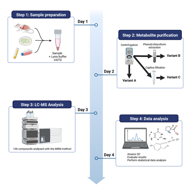
Figure 1 presents a schematic overview of the sample preparation process. Prior to initiating the sample preparation protocol, it is crucial to establish the required number of sample replicates. In our experience, strong inter-sample variation is frequent: 30%–40% of relative standard deviation for a given metabolite (comparison of biological replicates). This is almost exclusively caused by the experimental conditions and to a much lesser extent by several key steps in the protocol (see CRITICAL comments below). For example, animal diet or batch changes in the commercial serum used to culture cells will cause metabolism changes in laboratory animals or cells. Therefore, five biological replicates should be used when performing metabolomics analysis.

Figure 1.

Workflow of the general metabolite sample preparation and analysis

At the end of the sample preparation step (see custom-made protocols below), samples can be used straight away (i.e., metabolite purification step) or long-term stored (ideally overlaid with N₂) at −80°C (1 year in these conditions; longer storage times have not been tested).

Cell extracts

Timing: 30 min

The steps below describe the process of homogenizing cellular samples from cell culture.

• 4.
  Start from adherent cells (here we use HT29 cells) in 10 cm Petri dishes

  • a.
    Grow 3–5 million cells at 80% of confluence per dish.

    Note: Use RPMI cell culture medium supplemented with 10% FBS and 1% penicillin-streptomycin solution and a cell culture incubator at 37°C with humidified atmosphere containing 5% CO₂.

  • b.
    Wash the cell monolayer twice with ice-cold PBS (8 mL/wash).
  • c.
    Add 0.5 mL trypsin (trypsin-0.25% EDTA, phenol red) at 37°C for 5 min.

    • i.
      Stop the reaction with 10 mL culture medium (RPMI with 10% FBS).
    • ii.
      Dissociate cells by resuspension and collect them in a 15 mL tube (polypropylene screw cap, e.g., Corning cat. No. 352096 or similar).
    • iii.
      Count cells (cell number/mL), for instance with a Countess™ Automated Cell Counter or Bürker/Neubauer chamber and microscope.
  • d.
    Transfer 1 million cells to a fresh 15 mL tube.

    • i.
      Centrifuge at 200 g (swing-bucket rotor), 4°C, for 5 min.
    • ii.
      Remove as much as possible the liquid and add 10 mL of ice-cold PBS to the pellet.
    • iii.
      Centrifuge again (same conditions as before) and remove all PBS (as much as possible), keep the pellet.
  • e.
    Crush the pellet in 750 μL of ice-cold crushing solvent and transfer to a 1.5 mL polypropylene tube with a screw cap (e.g., Sarstedt cat. No. 72.687 or similar).

    • i.
      Add 0.5 g of glass beads (Retsch).
  • f.
    Homogenize the sample using the Precellys 24 tissue homogenizer (speed 4 m/s, 2 cycles of 15 s).

    CRITICAL: is crucial in step 4. Once cells leave the controlled atmosphere of the cell incubator, metabolism starts changing in an uncontrollable manner. This contributes to metabolite variability among replicates (discussed above). As enzymatic reactions stop when cells are crushed (step 4e), we suggest to handle a small number of samples at the same time in order to rapidly complete step 4 and to add the crushing solvent (step 4e) as quickly as possible (the actual number of samples will depend on the operator’s experience and the number of operators involved). Lastly, all PBS should be aspirated in step 4d because this will dilute the crushing solvent (thus increasing variability) and will introduce additional salts in the sample changing the sample matrix and hence cause retention time shifts in the analysis.

    Note: At step 4d, the remaining cells can be discarded or aliquoted (1 × 10⁶) in additional tubes to prepare technical replicates or back-up samples (in case of sample loss during the experiment).

Solid tissues (e.g., liver)

Timing: 60 min

The steps below describe the process of homogenizing animal tissue samples.

• 5.
  Start from fresh mouse tissues (liver or other organ/tissues) and proceed as follows:

  • a.
    Transfer the liver in a small Petri dish on ice, wash any visible blood by rinsing with ice-cold PBS. Discard PBS and remove excess PBS by blotting with filter paper. Cut liver into few small pieces (∼30 mm³) using scissors or a blade. Minimize time at room temperature or perform steps 1a and b in a cold room at +4°C.
  • b.
    Weigh the pieces on an analytical scale to have ∼50 mg/piece (10% tolerance; if more refer to the NOTE below) and rapidly transfer to 1.5 mL polypropylene tubes with screw cap. Add 0.5 g of glass beads.
  • c.
    Add 750 μL of ice-cold crushing buffer and homogenize the tissue using the tissue homogenizer Precellys 24 (speed 4 m/s, 2 cycles of 15 s).

CRITICAL: is crucial in step 5a. Determine the number of samples that can be efficiently processed with the available resources (e.g., number of operators involved). If handling more than 10 samples, prepare the 1.5 mL polypropylene tubes with 0.5 g of glass beads and 750 μL ice-cold crushing buffer in advance. Transfer the tissue directly into the pre-prepared tubes and keep them on ice for less than 30 min before mechanical homogenization. When crushing with mortar and pestle (for harder tissues, such as bone), we suggest first to snap freeze the tissue in liquid nitrogen, wrap it in aluminum foil for crushing in the mortar to avoid sample contamination and sample loss (all equipment coming in contact with the tissue must be pre-chilled in liquid nitrogen). All items that come into contact with the tissue powder must be rinsed with de-ionized water and wiped dry before re-use.

Note: The sample quantities indicated in the present protocol are the recommended and tested quantities that have given good results with the described LC-MS equipment. Aim for these sample amounts with minimal variations (±10%) among samples. If samples in one batch contain different amounts of starting material, we recommend to crush/lyse them in the same volume of crushing solvent (the ISTD should not be included in the crushing solvent at this step). Then, after step 2c (mechanical homogenization), the sample volume transferred to a new tube should be chosen in function of the sample weight (more volume for smaller samples and less for larger ones). Then, crushing solvent should be used to adjust the volume in order to have the same volume in all samples. At this point, one can spike with the ISTD before proceeding with the protocol. Importantly, when spiking, the final ISTD concentration should be 100 μM. To avoid large pipetting errors, an intermediate ISTD dilution should be prepared (in water) to have a spiking volume larger than 5 μL/sample.

Serum/plasma/cell culture supernatant

Timing:20 min(except the lyophilization step that takes 10–12 h)

The steps below describe the process of homogenizing liquid tissue samples and cell culture media.

• 6.
  For serum/plasma samples refer to step a below. Cell-free culture supernatants also can be used, but in this case the pre-made crushing solvent is not useful (see step 3b below).

  • a.
    Transfer 20 μL of serum or plasma sample to a 1.5 mL polypropylene tube with screw cap (see above) and add 750 μL of ice-cold crushing solvent.
  • b.
    From a 10 cm Petri dish (5 million cells at 80% of confluence), collect 250 μL of cell-free supernatant and add 500 μL of methanol and 5 μL of 100 μM ISTD (crushing solvent not needed).

Metabolite purification

For this step, one can choose among three protocol variants in function of the sample complexity. Cell lines or urine samples can be processed using the variant A, which also has the smallest cost. Tissues (incl. serum) require variant B or C, depending on the need to preserve proteins (only possible with variant B) and the safety considerations on the use of chloroform (variant C is chloroform-free). Moreover, variant C is adapted to the 96-well format and is suitable for high sample throughput. We performed head-to-head comparisons of the three protocol variants using cell pellets and did not observe any significant difference in performance. If cost is not an issue and protein recovery is not important, we recommend by default variant C.

Valid for all variants

Samples stored at −80°C (long-term storage) should be thawed and vortexed vigorously for 1 min (this step is omitted if using freshly prepared samples).

Variant A

Timing: 30 min (except the protein precipitation step that takes 10–12 h)

The steps below describe the purification of metabolites from cell extracts and cell culture supernatants.

• 7.Place fresh samples at −20°C for 10–12 h to precipitate proteins (not needed for samples stored at −80°C).
• 8.Centrifuge samples at 20,000 g/4°C for 15 min.
• 9.Remove supernatants and transfer them to a fresh 1.5 mL tube.
• 10.Dry samples in a SpeedVac.

CRITICAL: Proceed rapidly through steps 7–10, the protocol should not be paused except at step 7 (samples can be kept at −20°C for several days).

Note: After supernatant removal in step 9, a white protein pellet should be present at the bottom of the tube. This pellet needs to be removed for the subsequent analysis. The protein pellet can be dried at room temperature for 2 min under a fume hood and used for proteomics/western blotting. For this, the protein pellet should be re-suspended in the appropriate crushing solvent (e.g., 200–300 μL of 50 mM Tris-HCL, 1% SDS, pH 8.5). The protein content can be quantified with the bicinchoninic acid (BCA) protein assay. The necessary material is listed in the key resources table above.

Variant B

Timing: 1 h

The steps below describe a universal approach for the purification of metabolites from tissue samples, with the possibility of concomitant isolation of proteins. However, the method necessitates the utilization of chloroform.

• 11.Add 400 μL chloroform to the samples (prepared as described above).
• 12.Vortex samples vigorously for 1 min.
• 13.Centrifuge samples at 20,000 g/4°C for 15 min. Two distinct phases will be visible (lower chloroform and upper methanol/water phase).
• 14.Remove the methanol/water (upper) phase and transfer it in a fresh 1.5 mL tube.
• 15.Proceed to SpeedVac to dry the methanol/water phase.

Note: After step 13, a white protein layer is present in the interphase (between chloroform at the bottom and the upper methanol/water phase). This layer must not contaminate the sample for the subsequent analysis, but it may be collected, as described above, for proteomics/western blotting. Before proceeding, wash the layer to eliminate the residual chloroform in 1 mL of ice-cold acetone, centrifuge at 20,000 g, 4°C for 15 min, remove the supernatant and proceed to protein lysis as described in the NOTE above.

Variant C

Timing: 30 min (1 h if steps 1 and 2 are not skipped)

The steps below describe a universal approach for the purification of metabolites from tissue samples. The method is adapted for high-throughput processing.

In this variant, proteins are removed with the Captiva EMR plate. Therefore, if protein isolation is not a requirement, step 16 can be omitted. Samples can be still centrifuged as described in step 17 if they contain visible debris (this will be the case for tissues). For cell culture and serum samples, step 17 can be omitted and samples can be directly loaded in the Captiva EMR wells, as described in step 18 below.

• 16.Place samples at −20°C overnight to precipitate proteins (omitted if samples were stored at −80°C).
• 17.Centrifuge samples at 20,000 g/4°C for 15 min.
• 18.Collect the supernatant and transfer it to the Captiva EMR plate assembled on the Vacuum Manifold together with the Deep Well collection plate.
• 19.Apply low vacuum (−10 to −20 kPa) and allow samples to flow through the plate into the collection plate.
• 20.Remove the collection plate and place it in a SpeedVac to dry the samples.

Note: If protein precipitation was performed, protein pellets can be collected after centrifugation (step 17) and used as described above for proteomics/western blotting.

Pause point: For all variants, dried samples can be overlaid with N₂ and long-term stored at −80°C (1 year at least).

LC-MS/MS analysis

Preparation of solvents and LC-MS/MS set-up

Timing: 30 min

• 21.Prepare 4 solvent mixtures for the Agilent Infinity II UHPLC (used in this protocol): A and B (for the analytical gradient), Needle Wash (for rinsing the needle for sample injection), and Seal Wash (for rinsing the pump seals). The same set-up is available on all standard HPLC systems from major commercial vendors.

Solvent A: water/0.1% formic acid

Chemical	Amount
Water	1000 mL
Formic Acid	1 mL

Solvent B: acetonitrile/0.1% formic acid

Chemical	Amount
Acetonitrile	1000 mL
Formic Acid	1 mL

Needle Wash: methanol/water 50/50 and 0.1% formic acid

Chemical	Amount
Methanol	500 mL
Water	500 mL
Formic Acid	1 mL

Seal Wash: methanol/water 10/90 and 0.1% formic acid

Chemical	Amount
Methanol	100 mL
Water	900 mL
Formic Acid	1 mL

Note: All the above recipes are for 1 L of each solution (enough for at least 200 injections). However, we recommend to prepare fresh solutions for each experiment by calculating the required amount (plus 20% as safety margin). The required amounts of solvents A and B can be easily calculated by multiplying the number of injections to be performed (including blanks and QCs) by 0.25 mL (flow rate per minute) and by 25 min (duration of one analysis). The resulting volume is then increased by 20% and divided by two to obtain the volume of solvents A and B.

CRITICAL: If solutions are kept in bottles for more than 10 days, they will deteriorate. Moreover, algae and fungi may start to grow, particularly in solvent A. Atmospheric CO₂ will change their pH. Solvent B is light-sensitive because acetonitrile in acidic conditions tends to polymerize. We strongly recommend the use of brown bottles at least for solvent B (see key resources table). If large volumes are stored for long time, we recommend to remove the bottles from the HPLC station and store them at 4°C.

MS parameter optimization

Timing: 4–16 h (including possible automatic steps performed overnight)

Before starting the experimental sample analysis, it is important to optimize compound-dependent parameters (e.g., collision energy (CE)), which depend on the physical features of each measured molecule, and compound-independent parameters (e.g., source parameters), which are mainly influenced by the solvent composition and flow rate (and thus affect all compounds).

• 22.Adjust the CE for the individual MRM transitions. For Agilent 64xy triple-quad instruments (e.g., 6495C), the MRM CE described in this protocol (see Table S1: MS parameters and MRM transitions, related to MS Parameters Optimization section) can be used. Instruments from other vendors will require CE adjustments. In this case, CE can be optimized using direct injection (flow-injection analysis) and a mix of compounds included in the Compound List (mix a maximum of 10 compounds in one sample to perform CE optimization, then proceed to the next group). The compounds optimized in one mix must have different masses (at least 1 Da, but we recommend at least 2 Da).
• 23.Adjust the source parameters. If the source presented here (Agilent Jet Stream) is not used, individual optimization must be performed considering the solvent composition and flow rate (please, refer to the User Manual of the used instrument). After optimization of gas temperature, sheath gas temperature and flow, the next optimization step concern the iFunnel values on Agilent 6495 instruments to improve the performance. However, a compromise setting can be used for all compounds (therefore, compound-independent). To optimize the iFunnel refer to the 6495 series user manual. Importantly, iFunnel parameters only apply to the 6495 series, and other series (e.g., 6475) may not have this feature. Therefore, for these instruments, the iFunnel parameter optimization can be skipped.

Source Parameters

Gas temperature	250°C
Gas Flow	12 L/min
Nebulizer	35 psi
Sheath Gas Temperature	400°C
Sheath Gas Flow	12 L/min
Capillary Voltage (neg. mode)	4000 V
Capillary Voltage (pos. mode)	4000 V
Nozzle Voltage	500 V
iFunnel
High Pressure RF	Pos: 150 V
	Neg: 90 V
Low Pressure RF	Pos: 60 V Neg: 60 V

Note: For users of Shimadzu 8040, 8050 and 8060 series instruments, a commercially available MS method file, which contains a similar set of analytes, is accessible from the instrument vendor (General Metabolites, Shimadzu).

• 24.Program the LC gradient in the analytical method.

LC-Gradient

Time (min)	B (%)
0	0
2	0
5	25
11	35
15	95
20	95
20.1	0
25	0
Flow Rate	0.250 μL/min
Oven Temperature	40°C
Autosampler Temperature	8°C

Note: If the MS instrument has a divert valve, it can be used to divert the flow from the MS to waste after 15 min. This will ensure that the instrument remains operational longer, thus reducing the need of instrument cleaning.

For more information on the LC and MS parameters, please refer to the Supplemental section.

Compound list of 106 general metabolites measured with the present method.

Systems performance check

Timing: 3 h

The steps below outline the procedure to acquire all controls as well as the sample, necessary for evaluating the performance of the analysis.

Before starting the analysis of experimental samples, the LC-MS system performance needs to be verified. At this step, all retention times (RT) and CEs should have been properly included in the instrument method file.

For the system performance check, the following samples need to be prepared in LC-MS vials.

• 25.10 μL of 10 μM QC mix in water prepared from the MS Standards described in the Supplemental section Table S2.
• 26.Blank sample (add 100 μL of water to the prepared blank).
• 27.Positive control (add 100 μL of water to the prepared positive control).
• 28.Vortex samples vigorously for 1 min.
• 29.Transfer samples in LC-MS vials (Agilent, cat. # 5190-2242).
• 30.Inject 1 μL of each sample into the LC-MS system.

Note: Using all molecules listed in Supplemental section Table S2 to prepare the QC is ideal, but may not be practical because of the high cost of procuring all the standards. For routine QC, few molecules can be selected by making sure that they are evenly distributed along the chromatographic gradient.

• 31.Verify the performance check results by confirming the absence of signal for the blank sample, as outlined in Table S3 (if significant traces of metabolites listed in Table 1 are present, refer to the troubleshooting section below). Signals close to background are considered normal for some compounds because they are abundant and may be present as contaminants. Then, examine the QC mix result, as outlined in Table S4, and check that the tested compounds elute at the expected RT with the expected intensities and signal-to-noise (S/N) ratio (for RT shift problems, refer to the troubleshooting section). For obtaining reference values refer to the NOTE below. For more information on the S/N ratio calculation and interpretation, see the article by J.W. Dolan.⁷
• 32.Verify the results for the positive control sample. If using the same cells as in the present protocol, verify that the majority of metabolites listed in Table S5 and Figure 4 are present; otherwise, refer to the troubleshooting section. In case of other LC-MS system issues, refer to the troubleshooting section for the most common ones and how to solve them. Note that the RT in the positive control may vary (usually ± 0.2 min) compared with the QC. This is due to the presence of matrix in the positive control sample. More details are given in the “expected outcomes” and “troubleshooting” sections.

Note: Each MS system has its own sensitivity and performance features. Therefore, we cannot provide universal values (i.e., absolute intensities) for the system performance check. In this context, it is more important to establish the “normal” performance of the available instrument (ideally just after preventive maintenance, when performance and function have been verified), record the obtained values, and each time compare the new values with the recorded values. In this manner, each laboratory can define its own QC parameters, quickly spot problems and system deteriorations, and avoid the loss of precious samples in case of problems.

Figure 4.

In rare events, the largest peak may not represent the studied molecule, as shown here for citrulline

LC-MS/MS sample analysis

Timing: 30 min/sample

If the performance check results are satisfactory, proceed to the actual sample analysis.

• 33.Resuspend all dry samples in 100 μL of water.
• 34.Vortex samples vigorously for 1 min.
• 35.Transfer samples in LC-MS vials (Agilent, cat. # 5190-2242).
• 36.Inject 1 μL of sample onto the LC-MS system.

Note: Ideally, the sample injection sequence should be randomized. After the last sample, inject again blank, QC mix, and positive control to verify the performance. Injection of pure water between samples to check for carryover should be avoided because this may cause an RT shift for some molecules in the next sample. If a carryover check is needed (i.e., injections between experimental samples), the matrix-adjusted blank should be used because it will not affect the RT of the next sample. The sample injection volume can be increased safely to 10 μL without significant RT changes. The injection volume should be increased if the quantities of starting materials are below the amounts indicated in the Sample preparation section. Assuming that all samples in the experimental batch are similar in terms of type and quantity of starting material, we recommend to perform first a test injection using one random sample. This test allows determining the quantity that does not saturate the MS system and that is safe to use for the entire sample batch. If using the 6495C MS system, avoid signal intensities >10⁷ counts per second.

Expected outcomes

Although the method can measure all metabolites listed in Table 1, its sensitivity for each compound is different. Depending on their abundance in a sample, some of these compounds will be below the detection limit. The analysis of a typical biological sample (e.g., human cancer cells or tissues) gives data on ∼70–80 compounds among the 106 measured. In these samples, the highest sensitivity is for amino acids, and the lowest is for some metabolites of the Krebs cycle, such as alpha-ketoglutarate. For other molecule classes, nucleotides and nucleosides are generally well detectable, and also mono-phosphorylated nucleotides (the most difficult is thymidine monophosphate).

For some compounds (leucine/isoleucine, lysine, citrulline, glutamine and symmetric dimethylarginine), two close peaks are observed. Standard injections and spike-in (see “troubleshooting” section below) are necessary to identify the correct peak, because sometimes it is not the largest peak. Moreover, general metabolite preparations contain a rich organic and inorganic matrix (salts), causing frequent retention time drifts (± 0.2 min). These require additional, sample-dependent, confirmations. Examples are provided in the Figures 2, 3, and 4.

Figure 2.

Example of the measurement of isoleucine and leucine

Figure 3.

Example of two adjacent peaks that require further confirmation using QC and spike-in to determine which peak corresponds the studied molecule

To illustrate a typical metabolomics experiment, we incubated 60%-confluent HT29 colorectal cancer cells with/without (control) 10 μM metformin for 48 h, and then acquired/analyzed the metabolomic perturbations using the present protocol. The raw and ISTD normalized data are presented in the Table S5 section. We acquired also the corresponding blanks and QC measurements at the beginning, in the middle, and at the end of the acquisition batch (see Table S3 and Table S4). We processed the ISTD-normalized raw data using the MetaboR script (https://github.com/DirtyHarry80/MetaboR). Figure 5, below, shows the plots generated using the script and this dataset.

Figure 5.

Example of data analysis using the MetaboAnalystR package and the MetaboR script

The figure shows the metabolite quantification data for HT29 cancer cells after incubation or not with 10 μM metformin.

(A) PLS plot outlining control (HT29_Ctrl) and metformin-treated cells (HT29_Met).

(B) Volcano plot showing metabolites with at least 2-fold changes in concentration between conditions (HT29_Ctrl and HT29_Met).

(C and D) (C) Heatmap and (D) Correlation matrix of all compounds in the dataset.

Then, we performed the absolute quantification of 4-aminobutyric acid, glutamine and tryptophan in the HT29 Ctrl and Met samples. The calculation details are outlined in Supplemental section, Table S6. Figure 6 shows tryptophan quantification.

Figure 6.

Absolute quantification for tryptophan in the low μM range.

(A) tryptophan calibration curve consisting of quadruplicate measurements of diluted standard. Solid black points indicate values retained for the construction of the curve, while empty circles are excluded values.

(B) tryptophan quantification in HT29 cell extracts. Error bars indicate standard deviation of means from N=5 and N=6 biological replicates in HT29 Ctrl and HT29 Met conditions, respectively.

The raw data and calibration curves/evaluations for 4-aminobutyric acid and glutamine are in the Supplemental section, Table S6.

Quantification and statistical analysis

Basic data analysis

For relative quantification, the peak areas obtained for each compound are subtracted from the blank measurement and then divided by the ISTD area measured in that sample. Instead of subtracting its signal, the blank can be used to select the metabolites for further analysis (i.e., all metabolites significantly above the blank). The significance should be decided based on statistic testing (e.g., t-test) and a fold-change threshold (we suggest at least factor 10). Agilent users will require the Mass Hunter Workstation Quantitative Analysis software to perform peak integration, blank subtraction, and ISTD normalization. Similar software is provided by other vendors (e.g., Chromeleon for Thermo MS or LabSolutions for Shimadzu MS). Once calculated, these values are the normalized area values that can be averaged among replicates and used to compare individual samples in a relative fashion (Supplemental section, the Table S5). Following ISTD normalization, if reporting small numbers with decimals is an issue, these values can be scaled across all samples by multiplying them by a specific factor (e.g., 1000).

Note: ISTD normalization is only the first step in the data analysis, and this normalization only intends to correct volume errors that may have occurred during sample preparation. Normalization will work well as long as the matrix complexity is the same among samples (e.g., same type of cell line is compared with different treatments). When comparing samples with different matrices (e.g., serum versus cell culture supernatant) ISTD normalization should be skipped (as disadvantages will outweigh the advantages of using the ISTD). The ISTD-based normalization also does not account for signal suppression due to matrix variations or for experimental shortcomings (e.g., a drug might be slightly more efficient in one replicate than in another; slightly variable treatment timing). These variations need to be normalized using other means, as outlined in the “Comparison across multiple conditions” section below.

For absolute quantification, separate measurements of standards and their dilutions must be performed using the same analytical method. Two absolute quantification approaches can be proposed: semiquantitative and absolute.

Semiquantitative modality (used here): Non-isotopically labeled standards (diluted in water to obtain different concentrations) are used to generate the external calibration curve. These standards do not undergo sample preparation and are separately measured by LC-MS. Curves are fitted to the calibration points to describe the relationship between analyte area and concentration. The equations describing the curves are then used to calculate the quantities. Figure 6 and Table S6, show some examples.

Note: In this approach, the ISTD can be used to correct the areas among samples. To do so proceed first to build the area/ISTD ratios for each metabolite and sample as described in Basic data analysis. Define one random sample as reference and build correction coefficients for metabolites in all other samples. This is done by calculating a second ratio between area/ISTD values in a sample relative to this reference sample. Finally, use the correction coefficients to multiply with the measured areas in the samples and hence calculate the corrected areas in each samples. These are the areas used with calibration curves to quantify the metabolites. It is not worth to spike the ISTD in the external calibration curve because the ISTD signal intensity will be different compared with that of the actual samples due to the absence of complexity and matrix.

Absolute modality: The calibration curve is generated with isotopically labeled standards that are spiked at different concentrations directly in the calibration samples. Calibration samples should be obtained by pooling individual samples used in the study. For each sample (e.g., after sample crushing), a small aliquot is transferred to a separate tube and then all aliquots are pooled. Then, this pool is divided into individual tubes (one for each calibration point), and they are spiked with increasing concentrations of isotopically labeled standard. Calibration points and samples are both spiked with the ISTD (described above) and then processed for metabolite extraction. After the LC-MS analysis, the analyte area to ISTD area ratio is used to create the calibration curve (rather than just the analyte area, as done in the semiquantitative approach). For further details, see Duncan et al.⁸

Note: When performing the absolute quantification (using any of the above approaches), the quantity of a given metabolite must be reported relative to the original amount of input material. This is straightforward to understand when using serum. In this example, 20 μL of serum is used to start the sample preparation and at the end, the sample is diluted in 100 μL water before injecting 1 μL in the LC-MS system. Assuming that there was no sample loss during the different pipetting steps, only 1% of the original amount (or 0.2 μL of serum) is injected. Therefore, the absolute metabolite quantity measured in 1 μL of diluted sample must be multiplied by a dilution factor of 5 to scale the measurement to 1 μL serum or by a factor of 100 to scale to the original volume of 20 μL. The calculation is similar for cells and tissues, but some assumptions need to be made. For a measurement involving 1 × 10⁶ HT29 cells, we assume that the volume of 1 cell is 1000 μm³ or 1 × 10⁻¹² L. We also assume that each cell is made only of water. The volume of all cells in the sample is: 1 × 10⁶ × 1 × 10⁻¹² L = 1 × 10⁻⁶ L. If the final sample volume (before injection in the LC-MS system) was 100 μL, then the dilution factor is: 100 × 10⁻⁶ L/1 × 10⁻⁶ L = 100.

Comparison of multiple conditions

In experiments, different conditions (e.g., treated/untreated) are usually compared. Each sample group also includes different biological replicates. Therefore, a single normalization using only the ISTD may not be sufficient, because additional (e.g., biological and physical) effects may modify the actual metabolite intensities. An extensive overview of different normalization methods for metabolomics can be found elsewhere.⁹ A simple but effective method to normalize samples in these conditions is to blank-subtract and ISTD-correct the peak areas of each detected metabolite (as described in the basic data analysis section), followed by the final normalization (division) to the median, upper quantile or total signal intensity of all metabolites detected in the sample.

These analyses are efficiently done using dedicated R language packages, for example MetaboAnalystR.¹⁰ To provide an example on how to use MetaboAnalystR, we deposited an R script and a test dataset in the public repository GitHub, accessible at the following address: https://github.com/DirtyHarry80/MetaboR.git.

Note: To be used in MetaboAnalystR, data need to be saved as tab-delimited text files (decimals separated by a point) and must follow several criteria. For example, the R code lines, as outlined in MetaboR, will only work if the data table format respects a specific layout. For more details, see the MetaboR information on Github.

Depending on the data pre-normalization strategy, the function “Normalization” needs different parameter adjustments (in the MetaboR script, the parameters of “Normalization” are set to "QuantileNorm", "NULL", "AutoNorm" because we already normalized the data using ISTD and we wish to apply “QuantileNorm” and scale the data using "AutoNorm”).

MetaboR has an integrated outlier test based on Grubbs. The test will score each sample in the group (treatment or control) and based on the score value it allows identifying possible outliers that can then be removed manually from the analysis.

MetaboAnalystR offers a wide variety of graphical representations. In our opinion, the partial least squares regression (PLS) plot, volcano plot, heatmap and correlation matrix are the most useful (see Figure 5).

Limitations

One of the main limitations of the present method is obviously the number of metabolites it measures. The present list of 106 metabolites represents 40–60% of all molecules that may be measured with the present LC-MS method and modern MS instruments. Therefore, more works is needed to optimize and add additional molecules to the present method. This list will be certainly limited to molecules with medium hydrophobicity that in the present protocol will elute at retention times >7–8 min. In this chromatogram range, there is large potential for development. For example, some short chain fatty acids, polar lipids and poly-unsaturated fatty acids could be measured with the present LC-MS method. However, attention should be paid to the metabolite extraction protocol because it is not known which fraction of these new molecules can be extracted using the present crushing solvent. Like every method, the present protocol may produce variable results (coefficient of variation between 20%–40%) for the measured metabolites. This may occur with metabolites for which the sensitivity is rather low, as explained in the expected outcomes, because these compounds will be detected below the limit of quantification. Besides respecting the recommendations made in the notes at key steps of the protocol, increasing the number of full process replicates (biological replicates) is crucial to reduce the impact of result variability. Unexpected variations in some replicates can be then statistically detected using the Grubb’s test (included in the MetaboR script) and these samples can be removed from the analysis.

Troubleshooting

Problem 1

It is difficult to filter samples using the Captiva EMR plate (step 8).

Potential solution

Verify whether debris is present in the sample and if needed, centrifuge samples before loading in the Captiva plate. Do not increase the vacuum because samples need to flow slowly through the column (1 drop/s maximum).

Problem 2

Metabolite results are very variable among replicates (expected outcomes).

Potential solution

High metabolite variability can be explained by technical and/or biological causes. If a similar variability is not observed for the ISTD spiked in the samples, then a biological problem may be suspected. Confirm that after collection, samples were crushed in the extraction solvent as quickly as possible and that the sample, if stored before use, was stored correctly (at −80°C). The number of biological replicates may also be increased (at least 5 replicates should be prepared).

Problem 3

No flow from the HPLC (backpressure is < 10 bar, no liquid coming out of the capillary that connects the HPLC to the MS) (System performance check).

Potential solution

This may be due to air bubbles in the tubing from the bottle to the selection valves. Try purging the pumps. If the flow is not restarted, remove the solvent filters and test without them (regular cleaning in a sonication bath is necessary). Look for leaks between the bottle compartment and the pump. Check the pump seal wash solvent level (bottle empty?) and whether the wash is executed correctly. For this, start the seal wash and verify that the liquid flows through the tubing (usually made of transparent silicone material). If large bubbles are visible, repeat the seal wash or/and disconnect the last tubing and apply negative pressure using a syringe.

Problem 4

High pressure in the system (e.g., 10% or >160–170 bar, which is the usual value for this column at 0.25 mL/min, 9% solvent A and the used HPLC system) (System performance check).

Potential solution

To exclude column or/and capillary clogging, start by checking the MS system. This is done by removing one by one the capillaries that connect to the source and controlling the pressure. If the capillaries are not clogged, the pressure should drop by few bars at each step. If the pressure remains high after removing the column, clogging might be present until the pump. If the pressure drops significantly (pressure without the column should be ∼30 bar), the column might be clogged. Wash the column as described in problem 6, below, for 16 h (overnight). If the pressure is still high after this overnight wash, a column backflush might be performed to save the column by i) disconnecting the column and reversing the flow direction, ii) connecting the column-end to the waste directly, iii) injecting a 1:1:1 mix of isopropanol : acetonitrile : water at 45°C for 30 min (0.15 mL/min), and iv) reconnecting the column in the correct flow direction and use the initial method settings (90% A).

The column pre-heater, if used, also is a place where deposits may block the liquid flow, leading to pressure increase. Unmount the pre-heater and column and sonicate them separately in a methanol:water (50:50) solution under a fume hood for 20 min.

Problem 5

No signal or poor signal in the MS (System performance check).

Potential solution

First, to exclude any MS instrument-related problems, check the tune solution on the MS: make sure that the tune criteria set by the instrument vendor are met. If the tune criteria are not met, the instrument may need cleaning, particularly the spray unit in the source, cones, and transfer line. Refer to the instrument User Manual for the exact procedure.

Problem 6

Significant signal is detected in the blank sample (System performance check).

Potential solution

Perform the analysis using a pure water sample. If still positive, the cause is either a needle contamination or most probably a dirty analytical column. To clean it, purge pump A, and inject a freshly prepared isopropanol : acetonitrile : water (1:1:1) mix in the column (0.1 mL/min, 40°C oven temperature) for 16 h. Change the autosampler needle wash solution, wash, and purge. Inject at least 2–3 water samples, run the complete gradient (check that solvents A and B are correctly set). Repeat the measurement of the water sample and blank sample (process blank). If the water sample is negative and blank is still positive, check the sample preparation procedure (glassware and solvents may need to be cleaned/changed). If the water sample is still positive, perform a column backflush (invert the column flow and inject a 1:1:1 mix of isopropanol : acetonitrile : water, 0.15 mL/min at 60°C oven temperature for 30 min) to eliminate contaminants that may have accumulated in the column head (if this occurs frequently, use an appropriate pre-column mounted on the analytical column).

Problem 7

QC shows a retention time shift (System performance check).

Potential solution

Make sure that the HPLC solvents are not older than 1 week, and change them. If the shift is still present, check the pump volumetry and the indicated flow rates (they should correspond to the actual flow rates). Dead volumes in the connections after the column also can affect the chromatogram, particularly peak broadening and loss of separation when many compounds are eluted in a short time. Look for dead volumes (at the junctions of two capillaries, of capillary and valve, of capillary and column) by verifying the capillary connections after the column. Compare the pressure curve (during the run) with that of previous injections (e.g., instability, pressure increase). In the case of pressure instability, purge the pumps. If the problem persists, the column may need to be changed (a column of this type should usually last for 800 injections).

Problem 8

Few metabolites are identified in the sample (expected outcomes).

Potential solution

• •(sample with internal standard); The amount of starting material may have been too low. For cell samples, at least 2 × 10⁵ cells are required. Alternatively, the sample may be concentrated after the metabolite extraction step. Injecting more sample in the LC-MS is another option; however, the matrix load will also increase and ultimately cause column clogging, dirty source, and even contamination in the MS instrument.
• •(sample without internal standard); Check carefully the metabolite extraction steps. Verify that the protocol was followed correctly.

Problem 9

Fewer or additional peaks are visible for a given compound (expected outcomes).

Potential solution

For some metabolites, multiple peaks are normal and may indicate different isomers, as suggested for leucine and iso-leucine. However, for some metabolites, several unexpected peaks may be observed (see, for instance, Figures 3 and 4). In this case, check the retention time. This is done by spiking the expected compound as pure standard in the sample and by re-injecting the sample (use a small aliquot of the actual sample). The peak the intensity of which significantly increases is the correct peak.

Resource availability

Lead contact

Additional information and requests for resources (e.g., MS method file) and reagents should be directed to and will be fulfilled by the lead contact, Andrei Turtoi (andrei.turtoi@inserm.fr).

Materials availability

This study did not generate new unique reagents.

Data and code availability

The dataset supporting the current study has been included in Tables S3–S6 in the Supplemental section. The code used to create Figure 5 and the test dataset were deposited in the public repository GitHub, accessible at the following address: https://github.com/DirtyHarry80/MetaboR.git (https://doi.org/10.5281/zenodo.7962986). The instrument specific raw data are available from the corresponding author on request.

References

- 1.Costanza B., Turtoi A., Bellahcène A., Hirano T., Peulen O., Blomme A., Hennequière V., Mutijima E., Boniver J., Meuwis M.A., et al. Innovative methodology for the identification of soluble biomarkers in fresh tissues. Oncotarget. 2018;9:10665–10680. doi: 10.18632/oncotarget.24366. [DOI] [PMC free article] [PubMed] [Google Scholar]
- 2.Blomme A., Van Simaeys G., Doumont G., Costanza B., Bellier J., Otaka Y., Sherer F., Lovinfosse P., Boutry S., Palacios A.P., et al. Murine stroma adopts a human-like metabolic phenotype in the PDX model of colorectal cancer and liver metastases. Oncogene. 2018;37:1237–1250. doi: 10.1038/s41388-017-0018-x. [DOI] [PubMed] [Google Scholar]
- 3.Blomme A., Costanza B., de Tullio P., Thiry M., Van Simaeys G., Boutry S., Doumont G., Di Valentin E., Hirano T., Yokobori T., et al. Myoferlin regulates cellular lipid metabolism and promotes metastases in triple-negative breast cancer. Oncogene. 2017;36:2116–2130. doi: 10.1038/onc.2016.369. [DOI] [PubMed] [Google Scholar]
- 4.Guillon A., Brea-Diakite D., Cezard A., Wacquiez A., Baranek T., Bourgeais J., Picou F., Vasseur V., Meyer L., Chevalier C., et al. Host succinate inhibits influenza virus infection through succinylation and nuclear retention of the viral nucleoprotein. EMBO J. 2022;41:e108306. doi: 10.15252/embj.2021108306. [DOI] [PMC free article] [PubMed] [Google Scholar]
- 5.Stuani L., Sabatier M., Saland E., Cognet G., Poupin N., Bosc C., Castelli F.A., Gales L., Turtoi E., Montersino C., et al. Mitochondrial metabolism supports resistance to IDH mutant inhibitors in acute myeloid leukemia. J. Exp. Med. 2021;218:e20200924. doi: 10.1084/jem.20200924. [DOI] [PMC free article] [PubMed] [Google Scholar]
- 6.Turtoi E., Jeudy J., Valette G., Enjalbal C., Vila I.K., Laguette N., Turtoi A. Multiplexed targeted analysis of polyunsaturated fatty acids and oxylipins using LC-MS. STAR Protoc. 2023 doi: 10.1016/j.xpro.2023.102226. [DOI] [PMC free article] [PubMed] [Google Scholar]
- 7.Dolan J.W. The role of the signal-to-noise ratio in precision and accuracy. LC-GC Eur. 2006;19:12–16. [Google Scholar]
- 8.Duncan M.W., Gale P.J., Yergey A.L. Rockpool Productions LLC; 2006. The Principles of Quantitative Mass Spectrometry. [Google Scholar]
- 9.De Livera A.M., Sysi-Aho M., Jacob L., Gagnon-Bartsch J.A., Castillo S., Simpson J.A., Speed T.P. Statistical methods for handling unwanted variation in metabolomics data. Anal. Chem. 2015;87:3606–3615. doi: 10.1021/ac502439y. [DOI] [PMC free article] [PubMed] [Google Scholar]
- 10.Pang Z., Chong J., Zhou G., de Lima Morais D.A., Chang L., Barrette M., Gauthier C., Jacques P.É., Li S., Xia J. MetaboAnalyst 5.0: narrowing the gap between raw spectra and functional insights. Nucl. Acids Res. 2021;49:W388–W396. doi: 10.1093/nar/gkab382. [DOI] [PMC free article] [PubMed] [Google Scholar]
Associated Data
This section collects any data citations, data availability statements, or supplementary materials included in this article.
Supplementary Materials
Data Availability Statement