DeepSWI: Using Deep Learning to Enhance Susceptibility Contrast on T2*-Weighted MRI

Abstract

Background:

Although Susceptibility Weighted Imaging (SWI) is the gold standard for visualizing cerebral microbleeds (CMBs) in the brain, the required phase data are not always available clinically. Having a post-processing tool for generating SWI contrast from T2*-weighted magnitude images is therefore advantageous.

Purpose:

To create synthetic SWI images from clinical T2*-weighted magnitude images using deep learning and evaluate the resulting images in terms of similarity to conventional SWI images and ability to detect radiation-associated CMBs.

Study Type:

Retrospective.

Population:

145 adults (87males/58females; 43.9years-old) with radiation-associated CMBs were used to train (16,093patches/121patients), validate (484patches/4patients), and test (2420patches/20patients) our networks.

Field Strength/Sequence:

3D T2*-weighted, gradient-echo acquired at 3T.

Assessment:

Structural-Similarity-Index (SSIM), Peak Signal-to-Noise-Ratio (PSNR), normalized Mean-Squared-Error (nMSE), CMB counts, and line profiles were compared among magnitude, original SWI, and synthetic SWI images. Three blinded raters (JEVM, MAM, BB with 8-, 6-, and 4-years’ experience, respectively) independently rated and classified test-set images.

Statistical Tests:

Kruskall-Wallis and Wilcoxon signed-rank tests were used to compare SSIM, PSNR, nMSE, and CMB counts among magnitude, original SWI, and predicted synthetic SWI images. Intraclass correlation assessed inter-rater variability. P-values<0.005 were considered statistically significant.

Results:

SSIM values of the predicted vs original SWI (0.972,0.995,0.9864) were statistically significantly higher than that of the magnitude vs original SWI (0.970,0.994,0.9861) for whole brain, vascular structures, and brain tissue regions, respectively. 67% (19/28) CMBs detected on original SWI images were also detected on the predicted SWI, whereas only 10 (36%) were detected on magnitude images. Overall image quality was similar between the synthetic and original SWI images, with less artifacts on the former.

Conclusions:

This study demonstrated that deep learning can increase the susceptibility contrast present in neurovasculature and CMBs on T2*-weighted magnitude images, without residual susceptibility-induced artifacts. This may be useful for more accurately estimating CMB burden from magnitude images alone.

INTRODUCTION

Susceptibility-Weighted Imaging (SWI) has become the gold standard technique for visualizing iron containing structures such as veins and cerebral microbleeds (CMBs) in the brain, and remains a highly promising tool for assessing microstructural changes in iron content, tissue oxygenation, myelination, and vascular structure [1]. As such, the technique has been used extensively to detect and characterize pathology in patients with neurodegenerative disease, dementia, stroke, traumatic brain injury, and radiation therapy-induced vascular injury [2]. Enhanced susceptibility contrast is achieved by multiplying high pass filtered phase images with T2*-weighted magnitude images, where the phase mask highlights negative phase values arising from vessels and other high frequency structures [3]. The result is a further reduction of signal intensity in hypointense areas of the magnitude image that enhances the contrast of venous and other susceptibility-shifted structures [3].

When SWI processing is not directly available on the scanner, retrospective processing is contingent upon the saving of raw k-space data, complex-valued real and imaginary images, or phase images. This can hinder its widespread clinical use especially for multi-echo acquisitions where increased storage is required. Prior patents surrounding the processing and/or cost-prohibitive research packages have resulted in the interchangeable use of multi-echo magnitude T2*-weighted images with SWI, despite distinct differences in contrast and ability to detect lesions. For example, SWI is capable of detecting 31% (at 3T) and 54% (at 7T) more CMBs than the corresponding T2*-weighted magnitude images alone [4]. Standard SWI processing is also inherently prone to residual phase wrapping artifacts and susceptibility drop out around air-tissue interfaces, limiting its application in diseases involving the temporal lobes, surgical resection cavities, or other large lesions comprised of heterogeneous materials creating large susceptibility gradients [5].

With the growing popularity of SWI and pooling of data into larger multi-site studies, the need to retrospectively combining results quantified from SWI images with other T2*-weighted magnitude images from the same or similarly acquired sequence becomes of great importance. Since raw complex k-space data or phase images are not always saved along with the magnitude images in routine clinical T2*-weighted imaging, there currently is no way to create the more sensitive SWI image from the magnitude image alone, introducing large variability into such studies that could prevent a potentially relevant clinical finding from reaching statistical significance.

Synthetic image generation has been successfully applied in the field of medical imaging for a variety of different purposes. For example, Xiao et al. generated synthetic images in order to enhance the performance of spatial registration of different MR image modalities [6]. Other studies have generated synthetic Computed Tomography (CT) images from MR images for attenuation correction and radiation therapy planning, and Positron Emission Tomography (PET) images from CT images to increase sensitivity to detecting tumors [7][8][9]. Several researchers have also attempted to generate multiple MRI image contrasts such as T1-weighted, T2-weighted, and T2-FLAIR, using acquired contrasts and deep learning in order to reduce total scan time [10][11][12][13]. MR to MR image generation using convolutional neural networks has also been applied to obtain ultra-high magnetic field MR images (i.e. 7T) from lower magnetic field MR images (i.e. 3T) [14] [15], the results of which are often validated by improved performance on a segmentation task when using the synthetic higher field strength images. These studies show that deep neural networks can learn the nonlinear dependencies between different image modalities and contrasts.

Although generated synthetic MR images have been shown to improve computational operations such as image registration and segmentation, there has been limited evaluation on their ability to improve the quantification of metrics that are relevant in clinical applications [6] [13]. The lack of availability of SWI images ubiquitously in the clinic has also led to an underestimation of the number CMBs in larger studies of radiation-associated CMBs [17] compared to when SWI alone is utilized [18] because fewer CMBs are detected on magnitude T2*-weighted images. This study aimed to learn SWI contrast from T2*-weighted magnitude images alone using a generative adversarial network (GAN) framework and thereafter assess the network’s performance on CMB detection and quantification.

MATERIALS AND METHODS

Subjects and data acquisition

The retrospective study was conducted in accordance with the Declaration of Helsinki and approved by our Institutional Review Board. Informed consent was previously obtained from all patients involved in the study. 145 adult patients (87 males, 58 females; mean age 43.9 years old) who received prior treatment of a glioma and had confirmed radiation-associated CMBs on 3T SWI imaging that was performed as part of a research brain tumor imaging study were included in this study. 121 patients were used in training, 4 in validation, and 4 in testing.

3D T2*-weighted gradient echo (GRE) magnitude and phase MRI data were acquired on a 3T scanner (GE Healthcare Technologies, Milwaukee, WI, USA) with an 8-channel head coil (echo time (TE)/repetition time (TR)=28/46ms, flip angle=20, Field of View (FOV)=24cm, 0.625×0.625×2mm resolution, R=2 acceleration) in 145 patients with radiation-associated CMBs following treatment for glioma. SWI images were generated using traditional processing methods [19][3].

Image Preprocessing

3D patches of T2* weighted magnitude images, excluding regions of residual phase artifacts on SWI, were used as inputs in the training. Susceptibility-induced artifacts were manually masked, and erosion was applied to remove any edge artifacts. Voxel intensity values of all images were then normalized by dividing their intensities by 5 times the mode of the histogram of each image so that the resulting histogram peaks (reflecting background tissue signal intensity) were matched between the input magnitude and target SWI images and ranged from 0–1. Overlapping 3D input and target patches were created using magnitude and original SWI images (Figure 1B,C); alternative target patches were also created from the difference image (Figure 1D). The input patch size was 64×64xnumber of slices (with 16 overlapping voxels in each in plane direction) while target patches were cropped to 48×48 in plane to minimize any edge artifacts [20]. The effect of applying a hyperbolic tangent (tanh) transformation to the target patches to potentially facilitate model training by making the image distribution more Gaussian was also evaluated [20]. A semi-automatic CMB detection and segmentation algorithm [21] was applied to the magnitude and original SWI images to generate a mask of veins and segmented CMBs (Figure 1E,F); the resulting masks were integrated into the network to measure loss.

Figure 1. Image processing.

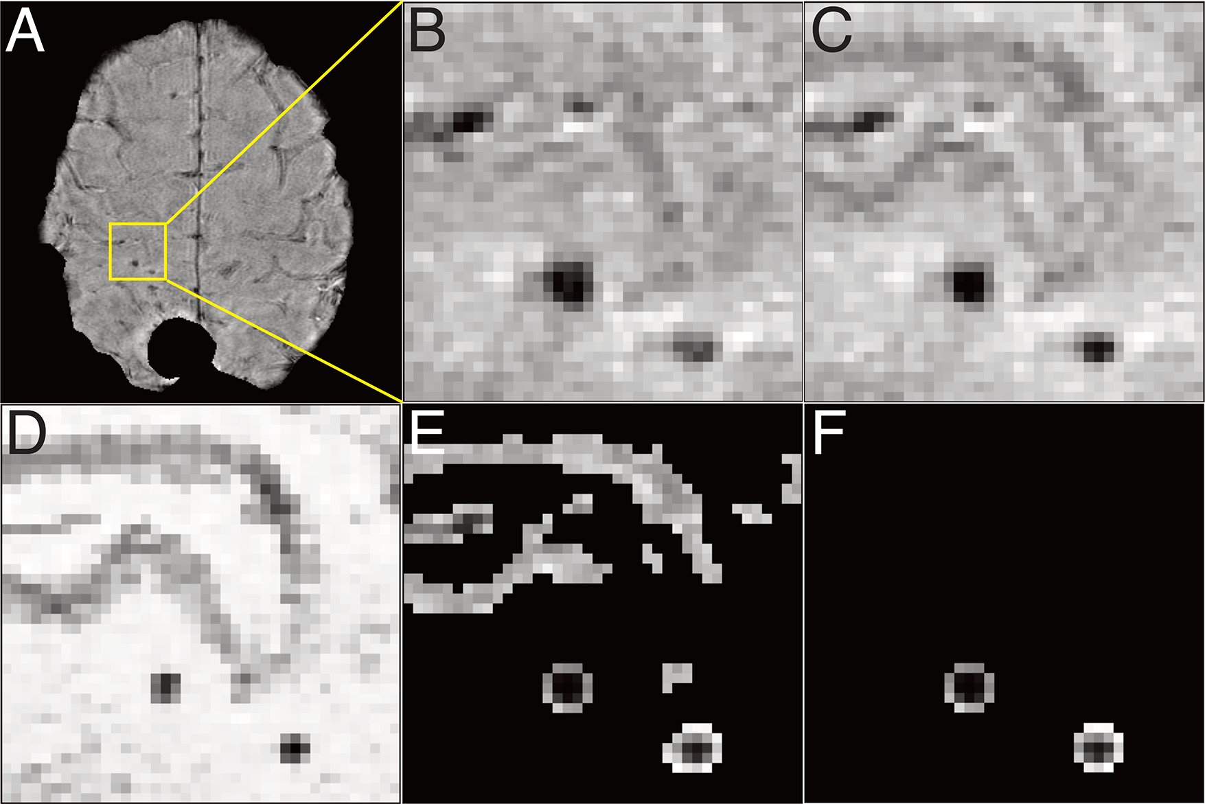
A. whole magnitude image, after removing artifacts due to a prior resection cavity and tumor for input in training. B. zoomed magnitude image, C. zoomed SWI, D. zoomed difference image of SWI and magnitude image, D. zoomed vessel and CMB-masked SWI, E. zoomed CMB-masked SWI.

Network Architecture

A conditional GAN technique with a fully convolutional U-Net as the generator network was employed [22]. Both the discriminator and the generator were conditioned on the input information to give a direction to the generation process as shown in Figure 2. This training approach enabled the generation of data distributions close to the sample data, and is advantageous for the proposed task because it allows for high frequency edges and structures to be captured [23].

Figure 2. Networks and training method.

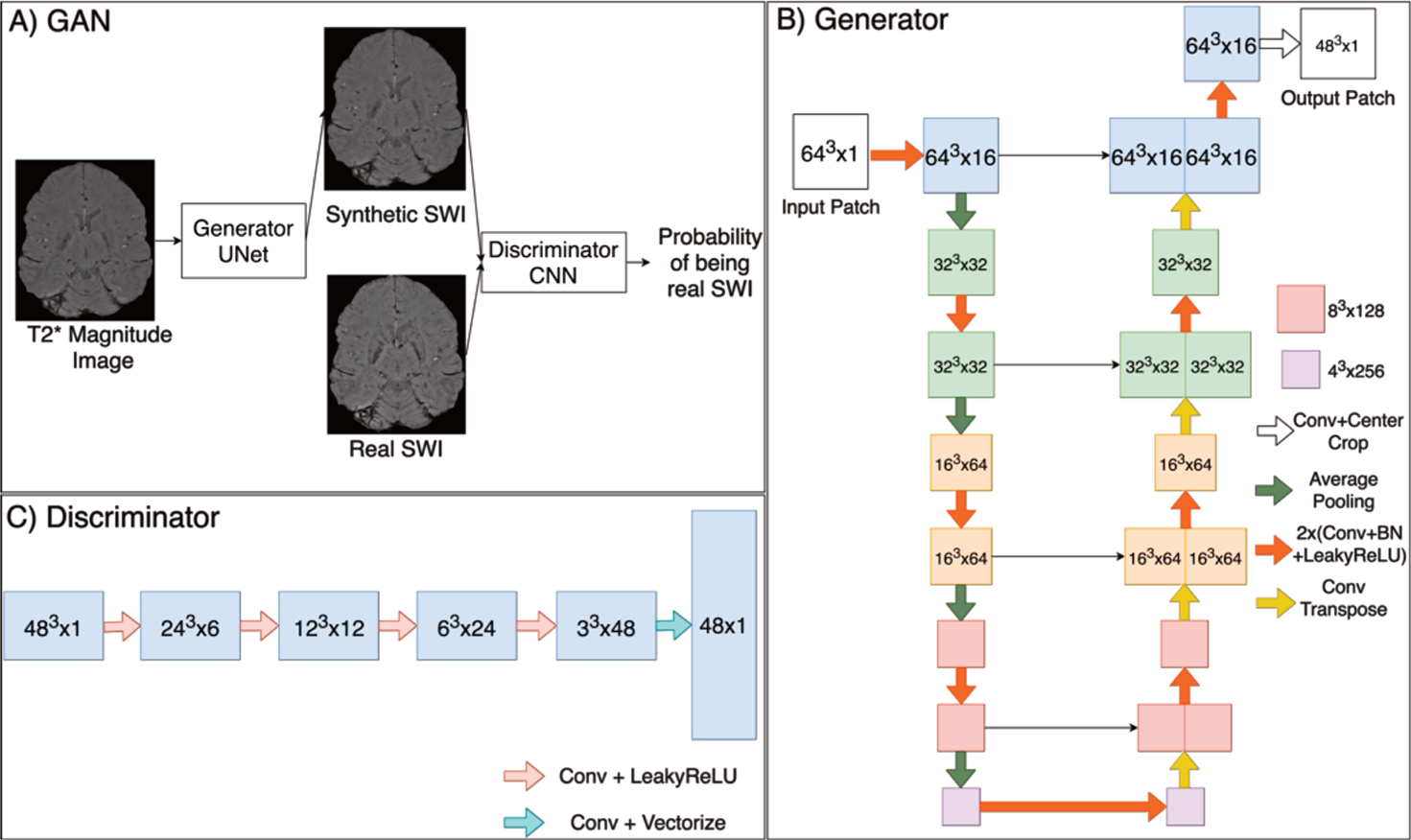
A. GAN, B. UNet Generator structure, C. CNN Discriminator structure.

Modified versions of the original GAN including the Wasserstein GAN with Gradient Penalty (WGAN-GP) [24] and Least Square GAN (LSGAN) [25] were implemented by adjusting the original GAN loss functions to either an Earth Mover (EM) loss that adds a gradient penalty to yield more stable training or least square loss for the discriminator instead of sigmoid cross entropy loss, respectively. These modified loss functions resulted in higher quality images and solved the vanishing gradient problem [26].

Hyperparameter Tuning with Bayesian Optimization

Hyperparameter values were initialized from Chen et al [20]. Bayesian Optimization was performed on the validation set via the open source Python package Optuna [27] to determine the optimal learning rate, batch size, number of channels, loss function of the generator network, model type, and whether or not to: 1) use the difference image as the output instead of the SWI image, 2) apply a tanh transformation to the voxel intensities so that their resulting distribution is more Gaussian, and 3) perform data augmentation that included flipping the image patches in all dimensions. The hyperparameter values maximizing mean Structural Similarity Index (SSIM) between the predicted and original SWI images within the region defined by the CMB mask of the validation set were used. The models were ran for 200 trials, training for 4000 iterations in each Bayesian Optimization trial.

Network Implementation & Training

Networks were implemented in Pytorch 1.5.1 and trained using NVIDIA GeForce RTX 2070, 8GB [20]. Two different GAN methods (LSGAN and WGAN-GP) were tested, with a 3D UNet as the generator, as well as the basic 3D UNet alone. 16,093 patches from 121 scans (83.4%) were used to train the network, 484 patches from 4 patients (2.8%) were used in validation, and 2420 patches from 20 scans (13.8%) were utilized for testing.

Each network was trained for 40,000 iterations with selected hyperparameters, including an Adam optimizer with initial learning rate of 0.009, beta1= 0.5, beta2 = 0.999. The combined mean absolute error (MAE) loss, mean squared error (MSE) loss and newly-defined CMB mask loss (Equation 1) was used for the generator, where masked loss represents the MAE between masked original SWI and masked predicted SWI. Coefficients of the loss terms (λ₁, λ₂, λ_masked) were tuned in Bayesian Optimization along with the other hyperparameters.

$$\begin{gathered} GeneratorLoss={\lambda }_1\ast \text{MAE}{\left(\mathrm{o}\mathrm{r}\mathrm{i}\mathrm{g}\mathrm{i}\mathrm{n}\mathrm{a}\mathrm{l}\mathrm{S}\mathrm{W}\mathrm{I},\mathrm{p}\mathrm{r}\mathrm{e}\mathrm{d}\mathrm{i}\mathrm{c}\mathrm{t}\mathrm{e}\mathrm{d}\mathrm{S}\mathrm{W}\mathrm{I}\right)}_{}+{\mathrm{\lambda }}_2*\mathrm{M}\mathrm{S}\mathrm{E}{\left(\mathrm{o}\mathrm{r}\mathrm{i}\mathrm{g}\mathrm{i}\mathrm{n}\mathrm{a}\mathrm{l}\mathrm{S}\mathrm{W}\mathrm{I},\mathrm{p}\mathrm{r}\mathrm{e}\mathrm{d}\mathrm{i}\mathrm{c}\mathrm{t}\mathrm{e}\mathrm{d} \\ \mathrm{S}\mathrm{W}\mathrm{I}\right)}_{}+{\mathrm{\lambda }}_{\mathrm{m}\mathrm{a}\mathrm{s}\mathrm{k}\mathrm{e}\mathrm{d}}*\mathrm{M}\mathrm{A}\mathrm{E}\left(\mathrm{m}\mathrm{a}\mathrm{s}\mathrm{k}\mathrm{e}\mathrm{d}\mathrm{o}\mathrm{r}\mathrm{i}\mathrm{g}\mathrm{i}\mathrm{n}\mathrm{a}\mathrm{l}\mathrm{S}\mathrm{W}\mathrm{I},\mathrm{m}\mathrm{a}\mathrm{s}\mathrm{k}\mathrm{e}\mathrm{d}\mathrm{p}\mathrm{r}\mathrm{e}\mathrm{d}\mathrm{i}\mathrm{c}\mathrm{t}\mathrm{e}\mathrm{d}\mathrm{S}\mathrm{W}\mathrm{I}\right) \end{gathered}$$ (Equation 1)

Evaluation and Statistical Analysis

A semi-automatic CMB detection algorithm was used to estimate the total number of CMBs on the test dataset [21] [28]. The number of CMBs detected, SSIM, peak signal-to-noise-ratio (PSNR), and normalized mean squared error (nMSE) were compared across magnitude, the original SWI, and predicted synthetic SWI images from the test set using a Kruskall Wallis or Wilcoxon Signed Rank test. Line profiles of individual CMBs and vessels of varying sizes were also visually compared across the magnitude, original SWI, and predicted synthetic SWI images. Three professionals (JEVM, MAM, and BB) with 8, 6, and 4 years’ respective experience identifying CMBs on SWI, were asked to classify and rate the overall image quality of 40 images (20 magnitude, 10 SWI_original, 10 SWI_predicted). Intraclass Correlation Coefficient (ICC) [29] was calculated to measure the reliability of these Likert ratings among the raters. P-values < 0.005 were considered statistically significant.

RESULTS

Hyperparameter Tuning

Four scans were sufficient for choosing 10 hyperparameters in an image generation task during validation because they resulted in 484 total patches, which included thousands of pixels predicted at once for each patch. Figure 3 shows the 10 hyperparameters tuned for training, including their search space, the final selected values (Figure 3A) and a plot of the SSIM values over the course of optimization trials (Figure 3B). Overall, the 169^th iteration yielded the highest SSIM value at 0.999921. Certain categorical hyperparameters performed better than others (Figure 4A). For example, batch sizes of 64, 16 or 8 along with 20, 24 or 16 channels for the generator resulted in higher SSIM values, and the LSGAN model type outperformed the basic 3D U-Net and WGAN-GP. Applying a tanh transformation of the output patch and learning the target image directly instead of the difference image increase the network performance, while data augmentation techniques did not improve network performance. SSIM values measured within the CMB-masked images and corresponding to iterations of Bayesian optimization with different continuous hyperparameters (i.e. MAE, MSE) were clustered together within the typical range of learning rates values (~0.005, 0.3) that tend to perform well (Figure 4B). A similar pattern was observed when setting the other categorical hyperparameters to the selected values and the continuous hyperparameters to the range of high SSIM yielding values (Figure 4B).

Figure 3. Overview of hyperparameter optimization.

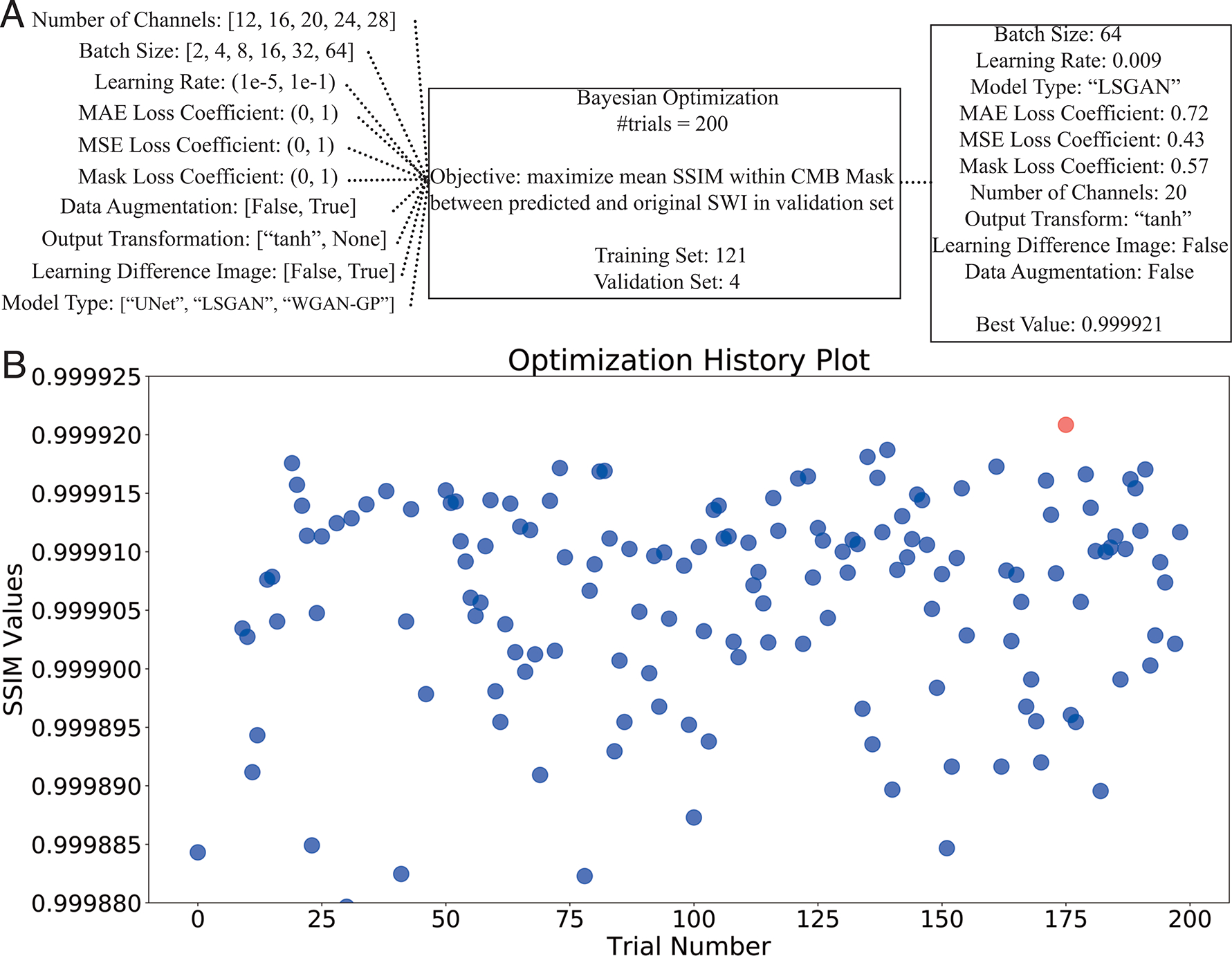
A. Search spaces for hyperparameter tuning (left) are shown with the final selected parameters (right). B. History plot of SSIM values across trials. Each blue dot represents a model training with different hyperparameter values. The red dot corresponds to the best experiment in the optimization process.

Figure 4. SSIM values across the hyperparameter search space.

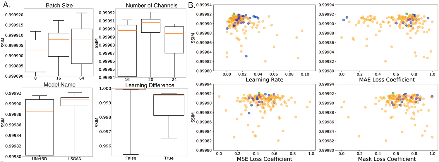
A. Categorical hyperparameters and corresponding SSIM between CMB-masked predicted and original SWI in the validation set. B. Continuous hyperparameters and corresponding SSIM values. Each dot corresponds to a different trial in the optimization process. Blue dots represent the experiments when other hyperparameters are in the range of high SSIM yielding values whereas light green dot represent the best experiment among all experiments.

Visual Evaluation

The predicted SWI yielded similar contrast to the original SWI images except for in the areas of residual phase wrapping artifacts (Figure 5A). Upon comparing the difference images in Figure 5, some of the small details were more prominent on the SWI_original – magnitude map. Figure 6A shows the violin plots of Likert ratings while Figure 6B shows the confusion matrices of classifications of each rater when asked to classify if an image was magnitude or SWI image contrast. For 18 of the 40 images classified, all raters agreed on the type of contrast. Although only 45% (9/20) of magnitude images, 60% (6/10) of original SWI images, and 20% (2/10) of predicted synthetic SWI images were correctly classified by all raters, the most experienced rater was able to correctly classify 80% (16), 80% (8), and 70% (7) of the magnitude, original SWI, and predicted SWI images, respectively. An ICC of 0.8 signified overall good agreement among the ratings of different raters.

Figure 5. Visual representation of the predicted SWI.

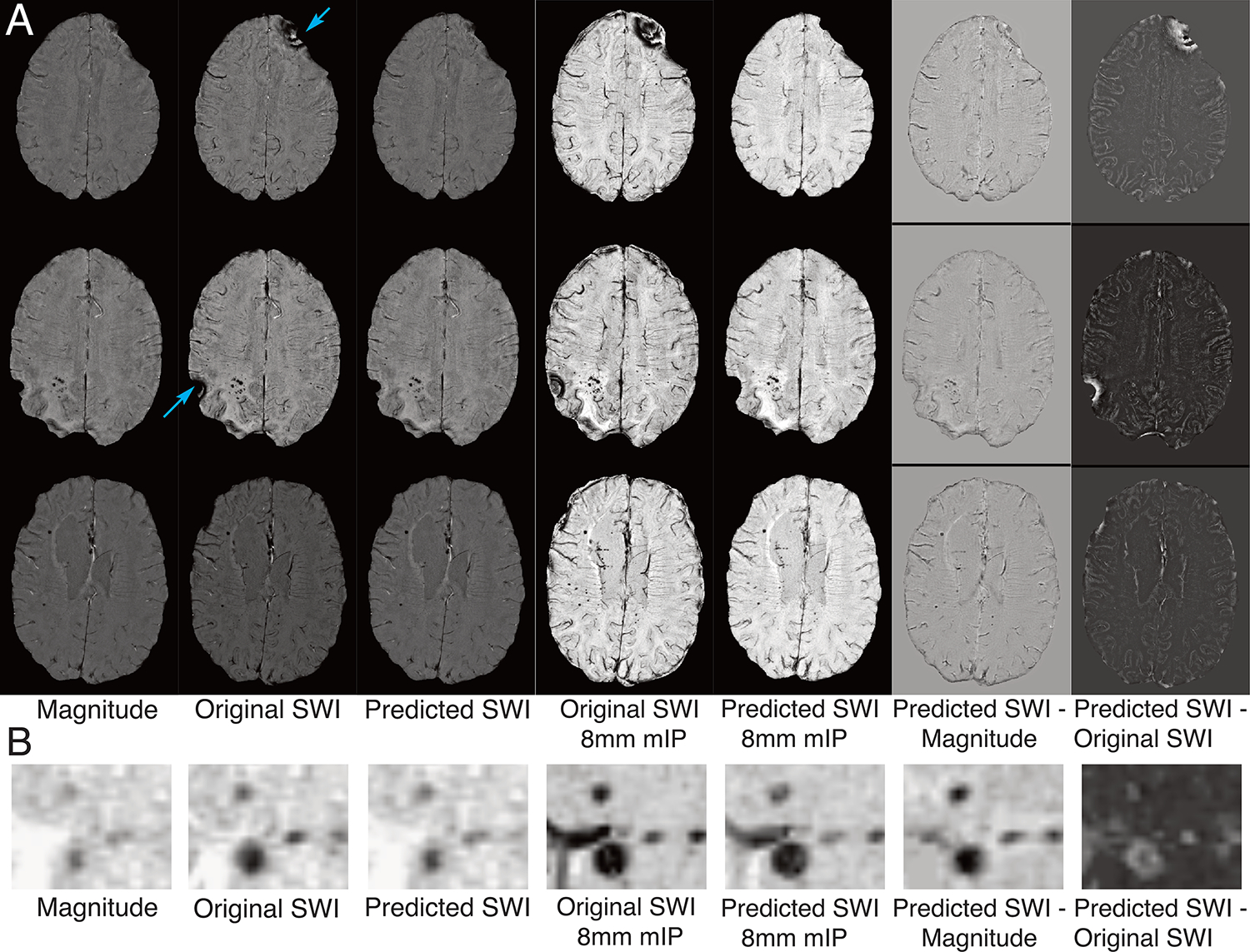
A. Representative multiple slice examples of the input magnitude image, original SWI, predicted SWI, their mIPs, and difference images from the predicted. B. Magnified view of the images in a region of small hypointense pathology.

Figure 6. Rating and Classification Results.

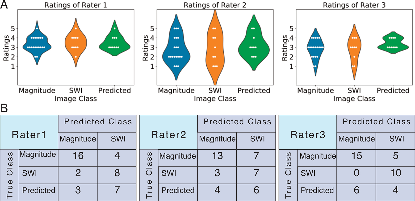
A. Violin plots of ratings. B. Confusion matrices of rater classifications.

Figure 7 depicts examples of a relatively poorly-predicted (Figure 7A,C) and well-predicted (Figure 7B,D) SWI image based on the total number of CMBs detected, spatial accuracy relative to the original SWI, and heightened CMB contrast. There was not a notable difference in the image quality of the magnitude or original SWI images between the two example synthetic images. Intensity values of small and large CMBs and vessels on the poorly-predicted SWI were in between that of the input magnitude and the original SWI, with the contrast of some small vessels on the predicted SWI similar to that of the input magnitude image (Figure 7D). Whereas in the well-predicted SWI, there were much larger differences in intensity across the images for all vascular structures, with similarly larger dips in the line profiles for both the original and predicted SWI images compared to the magnitude (Figure 7C).

Figure 7. Line Profile Analysis.

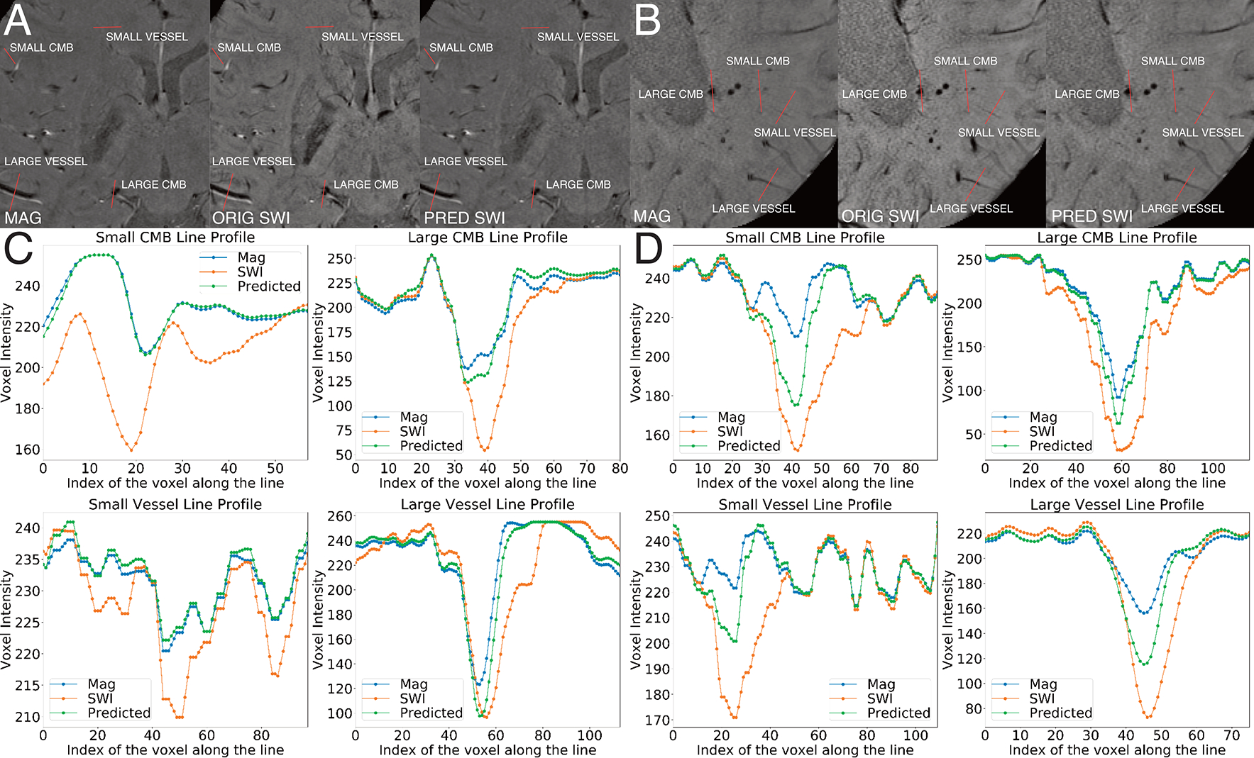
A and C are for CMB and vessel line profiles for a poorly predicted SWI. A. Input, original, and predicted images annotated in red along the trajectory of the line profile. C. Line profiles for a small CMB, large CMB, small vessel and large vessel. B and D are for CMB and vessel line profiles for a well-predicted SWI. B. Input, original, and predicted images annotated in red along the trajectory of the line profile. D. Line profiles for a small CMB, large CMB, small vessel and large vessel.

Comparison of Quantitative Metrics

Figure 8 shows boxplots of SSIM values of the predicted SWI vs original SWI, and the magnitude vs original SWI, for each scan in the test set. Mean values of SSIM, PSNR, and NMSE are listed in Table 1. Mean SSIM values of the predicted vs original SWI were statistically significantly higher than that of the input magnitude vs original SWI; this held true for the whole brain images (0.972 vs 0.970; Figure 8A), vessel and CMB-masked images (0.995 vs 0.994; Figure 8B), as well as areas outside of CMB and vessel masks (0.9864 vs 0.9861; Figure 8C). On average, 19 of the 28 CMBs detected on the original SWI images were also detected on the predicted SWI images, whereas only 10 of these (36%) were detected on the magnitude images, with significant differences in counts observed among all three image sets (Figure 8D).

Figure 8. Differences in SSIM values and CMB count across images.

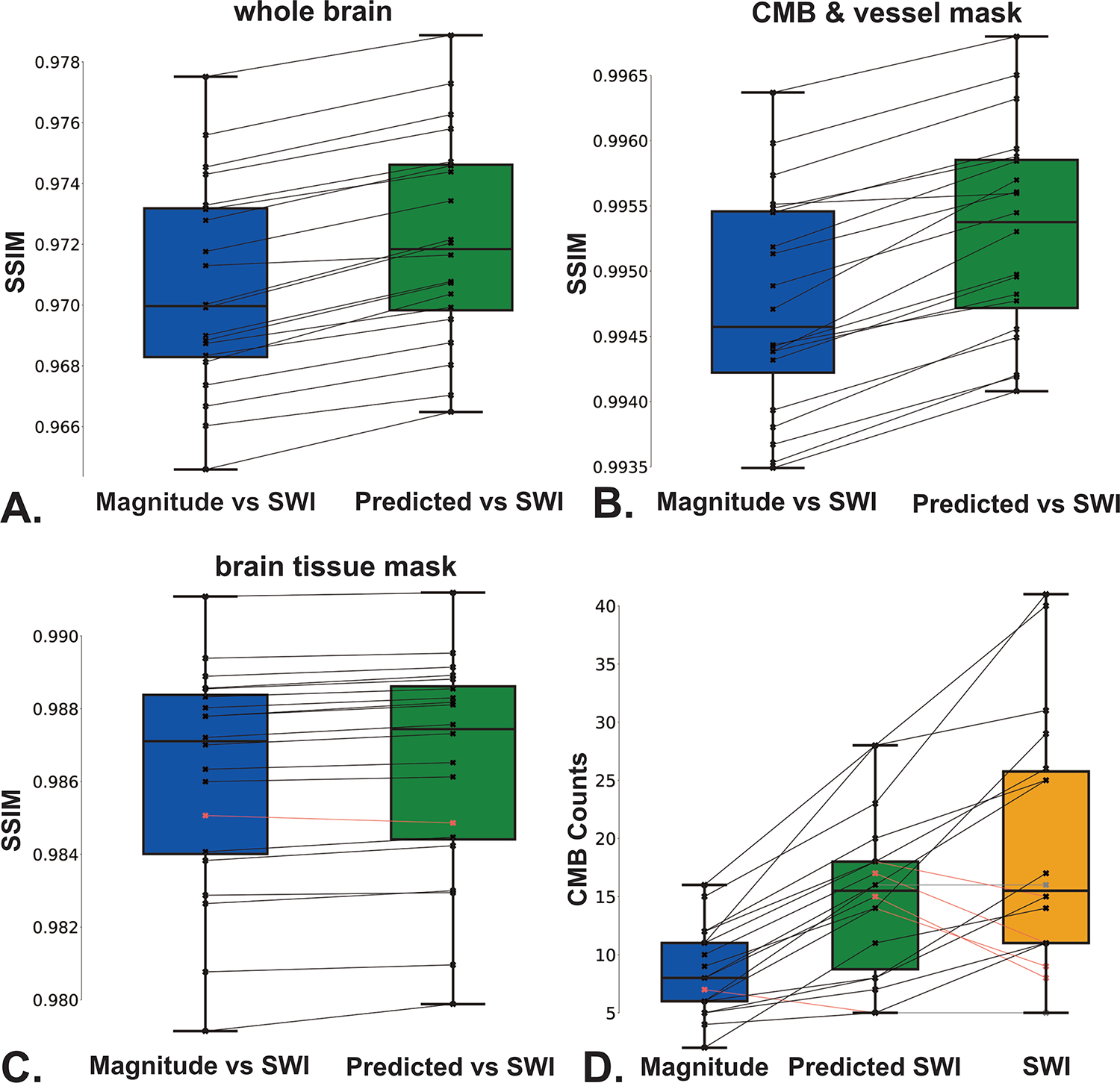
A-C. Comparison of SSIM values of the predicted SWI vs original SWI and magnitude image vs original SWI for (A) whole-brain images, (B) CMB and vessel-masked images, and (C) brain tissue masked images. D. Boxplots showing the number of CMBs detected on the input magnitude image, original and predicted SWI images using semi-automated detection.

Table 1.

Mean values of SSIM, PSNR and NMSE for the whole brain, vascular structures, and brain tissue regions from images in the test set.

Metric	Comparison	Whole Brain	Vascular Structures	Brain tissue
SSIM	M/O	0.970	0.994	0.9861
	P/O	0.972	0.995	0.9864
PSNR	M/O	37.693	40.087	39.067
	P/O	38.039	40.619	39.352
NMSE	M/O	0.013	0.056	0.0108
	P/O	0.012	0.049	0.0101

SSIM: Structural similarity index, PSNR: Peak signal to noise ratio, NMSE: Normalized mean square error, M/O = magnitude vs. original SWI, P/O = predicted vs. original SWI.

DISCUSSION

This work tested whether a conditional GAN training approach could be used to generate synthetic SWI images from T2*-weighted magnitude images in the absence of phase data. Unlike prior studies which have been limited to segmentation and classification problems, this study evaluated whether the synthetic images could retain similar susceptibility contrast to traditionally processed SWI for the detection of CMBs in a clinical population [6][14]. A conditional LSGAN with optimal hyperparameter values can learn the majority of additional susceptibility weighting produced by SWI processing when magnitude images serve as network inputs.

The hyperparameters evaluated in this study not only represented the parameter space of networks and their loss functions, but also determined the training workflow (e.g. data augmentation, and type of input patch and output transformation). By tuning all the parameters of the training workflow together, Bayesian optimization methods were applied to identify the best training strategy. Some of the hyperparameters such as data augmentation and MAE loss coefficient did not have a large impact on the objective values. Values for the latter were selected over a broader range than the MSE and mask loss coefficients, and therefore could indicate that MAE loss did not have as significant of an impact on our task. Data augmentation also did not improve the network performance, which could suggest that the network has seen enough data to learn the patterns and the augmented data did not provide extra information.

Performance was evaluated qualitatively and quantitative via an image similarity index and ability to detect CMBs. While the magnitude images were already relatively similar to the original SWI images, visually and quantitatively the predicted synthetic SWI images had more similar contrast to the original SWI than to the magnitude images. Regions of residual phase wrapping artifact on the original SWI did not appear on the predicted SWI, because artifact-free magnitude images as inputs and artifact free SWI images were intentionally used as targets, hence the network had not previously encountered these artifacts. Likert ratings demonstrated that the image quality of the predicted SWI images were equivalent to the original SWI and magnitude images. Although no statistically significant difference was found among the ratings of these image groups, a trend of slightly higher ratings was observed for the predicted SWI, perhaps due to the elimination of phase artifacts by our neural network. Although Raters 1 (a neuroradiologist) and 2 classified the majority of the predicted synthetic SWI images as original SWI images, Rater3 classified the majority of the synthetic SWI as magnitude images because they did not have the residual phase wrapping artifacts that they were accustomed to viewing with SWI. Quantitatively, mean NMSE and SSIM values were lower between the predicted and original SWI compared to the values between magnitude and original SWI, whereas the opposite was found for mean PSNR values. This further substantiates how the network is learning some of the target image contrast, resulting in realistic SWI image contrast.

Regardless of image quality, our network could learn most of the added hypointense susceptibility contrast of veins and CMBs generated by SWI processing. Line profiles showed that at the lowest voxel intensity value corresponding to the middle of the CMB, original SWI images are the most hypointense, followed by the predicted synthetic SWI images. A similar pattern was observed in the line profiles of large vessels irrespective of predicted synthetic SWI image quality, however, the line profiles of small vessel produced varying voxel intensities across the different images. This might indicate that the network could learn the target contrast of larger vessels better than smaller veins because of their relatively small sizes. When examining smaller CMB-like pathologies, small structures that were either missing or blurry on magnitude images were in fact present and more conspicuous on both the predicted and original SWI images, explaining the significantly increased number of CMBs detected overall on our synthetic SWI images compared to magnitude images. This is despite one subject whose CMB counts using the predicted SWI (n=5) were lower than both the magnitude (n=7) and original SWI (n=11). In another subject for comparison, however, 80% of CMBs (20/25) could be detected on the predicted SWI, while less than half (12/25) CMBs could be detected on the magnitude image.

Limitations

Although this work indicates that it is possible for a conditional GAN to learn susceptibility contrast weighting without the phase signal information, there is still room for improvement. One limitation is that all images in this study were acquired in a relatively small cohort with the same SWI acquisition protocol. Although our augmentation results suggest that adding more similar contrast images would not help performance of our network, including susceptibility weighted images acquired with a range of parameters, including various TE/TR/flip angles, resolution, and k-space sampling patterns, as well as data acquired with multiple echoes and from different field strengths such as more sensitive 7T scanners, could potentially improve performance, as well as further enriching our cohort with images from multiple sites and vendors. Other limitations of the study are that only GAN based approaches were employed and tuned only the most important hyperparameters with limited ranges. Although using a spatially-weighted loss function that focused on CMB locations when calculating SSIM resulted in artificially high values with small deviations during hyperparameter optimization due to the presence of zeroes in the mask having an SSIM of 1, without this approach, overall performance of the network and resulting synthetic image quality dropped. It is possible that future work constructing more complex neural networks, new hybrid approaches of CNNs, and transformer-based networks along with tuning more hyperparameters with larger options and ranges will improve upon the current results, but these approaches will likely require more time, computational resources, and techniques of parallel programming.

Conclusion

This study demonstrated the ability to increase the susceptibility contrast of T2*-weighted magnitude images using deep learning in the form of conditional GANs to generate synthetic SWI images. Both visual and quantitative analyses revealed that our network could learn the added susceptibility contrast present in both normal brain vasculature and CMBs without generating susceptibility-induced artifacts such as residual phase wraps. Although further improvement is still needed to match the full extent of SWI contrast, these synthetic images may be useful for more accurately estimating CMB burden of a patient in the clinic when the phase information was not saved, preventing the generation of SWI images using standard processing methods. While this work sought to address the logistical issue of unavailability of phase information with T2*-weighted acquisitions that is a common occurrence in clinical trials, modifications of this deep learning approach could also be used in the future to synthesize phase data from a shorter acquisition consisting of fewer echoes and shorter TEs.

REFERENCES

- [1].Bowers DC et al. , “Late-occurring stroke among long-term survivors of childhood leukemia and brain tumors: a report from the Childhood Cancer Survivor Study,” J. Clin. Oncol. Off. J. Am. Soc. Clin. Oncol, vol. 24, no. 33, pp. 5277–5282, Nov. 2006, doi: 10.1200/JCO.2006.07.2884. [DOI] [PubMed] [Google Scholar]
- [2].Halefoglu A and Yousem D, “Susceptibility weighted imaging: Clinical applications and future directions,” World J Radiol, vol. 10, no. 4, pp. 30–45, Apr. 2018. [DOI] [PMC free article] [PubMed] [Google Scholar]
- [3].Haacke E, Xu Y, Cheng Y, and Reichenbach J, “Susceptibility weighted imaging (SWI).,” Magn Reson Med, Sep. 2004. [DOI] [PubMed] [Google Scholar]
- [4].Bian W, Hess CP, Chang SM, Nelson SJ, and Lupo JM, “Susceptibility-weighted MR imaging of radiation therapy-induced cerebral microbleeds in patients with glioma: a comparison between 3T and 7T,” Neuroradiology, vol. 56, no. 2, pp. 91–96, Feb. 2014, doi: 10.1007/s00234-013-1297-8. [DOI] [PMC free article] [PubMed] [Google Scholar]
- [5].Li N, Wang W, Sati P, Pham D, and Butman J, “Quantitative assessment of susceptibility-weighted imaging processing methods.,” J Magn Reson Imaging, vol. 40, no. 6, pp. 1463–73, Dec. 2014. [DOI] [PMC free article] [PubMed] [Google Scholar]
- [6].Xiao S, Wu Y, Lee AY, and Rokem A, “MRI2MRI: A deep convolutional network that accurately transforms between brain MRI contrasts,” bioRxiv, p. 289926, Mar. 2018, doi: 10.1101/289926. [DOI] [Google Scholar]
- [7].Wolterink JM, Dinkla AM, Savenije MHF, Seevinck PR, van den Berg CAT, and Išgum I, “Deep MR to CT Synthesis Using Unpaired Data,” in Simulation and Synthesis in Medical Imaging, Cham, 2017, pp. 14–23. doi: 10.1007/978-3-319-68127-6_2. [DOI] [Google Scholar]
- [8].Leynes A et al. , “Zero-Echo-Time and Dixon Deep Pseudo-CT (ZeDD CT): Direct Generation of Pseudo-CT Images for Pelvic PET/MRI Attenuation Correction Using Deep Convolutional Neural Networks with Multiparametric MRI,” J Nucl Med, May 2018. [DOI] [PMC free article] [PubMed] [Google Scholar]
- [9].“Synthesis of Positron Emission Tomography (PET) Images via Multi-channel Generative Adversarial Networks (GANs),” springerprofessional.de. https://www.springerprofessional.de/en/synthesis-of-positron-emission-tomography-pet-images-via-multi-c/15033206 (accessed Apr. 27, 2021).
- [10].Chartsias A, Joyce T, Giuffrida M, and Tsaftaris S, “Multimodal MR Synthesis via Modality-Invariant Latent Representation.,” IEEE Trans Med Imaging, Mar. 2018. [DOI] [PMC free article] [PubMed] [Google Scholar]
- [11].Dar S, Yurt M, Karacan L, Erdem A, Erdem E, and Cukur T, “Image Synthesis in Multi-Contrast MRI With Conditional Generative Adversarial Networks.,” IEEE Trans Med Imaging, Oct. 2019. [DOI] [PubMed] [Google Scholar]
- [12].Wei W et al. , “Fluid-attenuated inversion recovery MRI synthesis from multisequence MRI using three-dimensional fully convolutional networks for multiple sclerosis.,” J Med Imaging (Bellingham), Jan. 2019. [DOI] [PMC free article] [PubMed] [Google Scholar]
- [13].Mani A et al. , “Applying Deep Learning to Accelerated Clinical Brain Magnetic Resonance Imaging for Multiple Sclerosis.,” Front Neurol, Sep. 2021. [DOI] [PMC free article] [PubMed] [Google Scholar]
- [14].Nie D et al. , “Medical Image Synthesis with Deep Convolutional Adversarial Networks,” IEEE Trans. Biomed. Eng, vol. 65, no. 12, pp. 2720–2730, Dec. 2018, doi: 10.1109/TBME.2018.2814538. [DOI] [PMC free article] [PubMed] [Google Scholar]
- [15].Sharma A, Kaur P, Nigam A, and Bhavsar A, “Learning to Decode 7T-like MR Image Reconstruction from 3T MR Images,” ArXiv180606886 Cs, Jun. 2018, Accessed: Apr. 27, 2021. [Online]. Available: http://arxiv.org/abs/1806.06886 [Google Scholar]
- [16].“Convolutional Neural Network for Reconstruction of 7T-like Images from 3T MRI Using Appearance and Anatomical Features,” springerprofessional.de. https://www.springerprofessional.de/en/convolutional-neural-network-for-reconstruction-of-7t-like-image/10832734 (accessed Apr. 27, 2021).
- [17].Roddy E et al. , “Presence of cerebral microbleeds is associated with worse executive function in pediatric brain tumor survivors.,” Neuro Oncol, Nov. 2016. [DOI] [PMC free article] [PubMed] [Google Scholar]
- [18].Morrison M et al. , “Rate of radiation-induced microbleed formation on 7T MRI relates to cognitive impairment in young patients treated with radiation therapy for a brain tumor.,” Radiother Oncol, Jan. 2021. [DOI] [PMC free article] [PubMed] [Google Scholar]
- [19].Lupo J et al. , “GRAPPA-based susceptibility-weighted imaging of normal volunteers and patients with brain tumor at 7T.,” Magn Reson Imaging, May 2009. [DOI] [PMC free article] [PubMed] [Google Scholar]
- [20].Chen Y, Jakary A, Avadiappan S, Hess CP, and Lupo JM, “QSMGAN: Improved Quantitative Susceptibility Mapping using 3D Generative Adversarial Networks with increased receptive field,” NeuroImage, vol. 207, p. 116389, Feb. 2020, doi: 10.1016/j.neuroimage.2019.116389. [DOI] [PMC free article] [PubMed] [Google Scholar]
- [21].Bian W, Hess CP, Chang SM, Nelson SJ, and Lupo JM, “Computer-aided detection of radiation-induced cerebral microbleeds on susceptibility-weighted MR images,” NeuroImage Clin, vol. 2, pp. 282–290, 2013, doi: 10.1016/j.nicl.2013.01.012. [DOI] [PMC free article] [PubMed] [Google Scholar]
- [22].Ronneberger O, Fischer P, and Brox T, “U-Net: Convolutional Networks for Biomedical Image Segmentation,” ArXiv150504597 Cs, May 2015, Accessed: Apr. 27, 2021. [Online]. Available: http://arxiv.org/abs/1505.04597 [Google Scholar]
- [23].Goodfellow IJ et al. , “Generative Adversarial Networks,” ArXiv14062661 Cs Stat, Jun. 2014, Accessed: Apr. 27, 2021. [Online]. Available: http://arxiv.org/abs/1406.2661 [Google Scholar]
- [24].Gulrajani I, Ahmed F, Arjovsky M, Dumoulin V, and Courville A, “Improved Training of Wasserstein GANs,” ArXiv170400028 Cs Stat, Dec. 2017, Accessed: Apr. 27, 2021. [Online]. Available: http://arxiv.org/abs/1704.00028 [Google Scholar]
- [25].Mao X, Li Q, Xie H, Lau RYK, Wang Z, and Smolley SP, “Least Squares Generative Adversarial Networks,” ArXiv161104076 Cs, Apr. 2017, Accessed: Apr. 27, 2021. [Online]. Available: http://arxiv.org/abs/1611.04076 [Google Scholar]
- [26].Wang Z, She Q, and Ward TE, “Generative Adversarial Networks in Computer Vision: A Survey and Taxonomy,” ArXiv190601529 Cs, Dec. 2020, Accessed: Apr. 27, 2021. [Online]. Available: http://arxiv.org/abs/1906.01529 [Google Scholar]
- [27].Akiba T, Sano S, Yanase T, Ohta T, and Koyama M, “Optuna: A Next-generation Hyperparameter Optimization Framework,” ArXiv190710902 Cs Stat, Jul. 2019, Accessed: Apr. 27, 2021. [Online]. Available: http://arxiv.org/abs/1907.10902 [Google Scholar]
- [28].Morrison MA, et al. , “A user-guided tool for semi-automated cerebral microbleed detection and volume segmentation: Evaluating vascular injury and data labelling for machine learning.” NeuroImage Clin, vol. 20, pp. 498–505, 2018, doi: 10.1016/j.nicl.2018.08.002. [DOI] [PMC free article] [PubMed] [Google Scholar]
- [29].Shrout P and Fleiss J, “Intraclass correlations: uses in assessing rater reliability,” Psychol Bull, Mar. 1979. [DOI] [PubMed] [Google Scholar]