Characterizing Streamline Count Invariant Graph Measures of Structural Connectomes

Abstract

Background:

While graph measures are used increasingly to characterize human connectomes, uncertainty remains in how to use these metrics in a quantitative and reproducible manner. Specifically, there is a lack of community consensus regarding the number of streamlines needed to generate connectomes.

Purpose:

The purpose was to define the relationship between streamline count and graph-measure value, reproducibility, and repeatability.

Study Type:

Retrospective analysis of previously prospective study.

Population:

Ten healthy subjects, 70% female, aged 25.3 ± 5.9 years.

Field Strength/Sequence:

A 3-T, T1-weighted sequences and diffusion-weighted imaging (DWI) with two gradient strengths (b-values = 1200 and 3000 sec/mm², echo time [TE] = 68 msec, repetition time [TR] = 5.4 seconds, 120 slices, field of view = 188 mm²).

Assessment:

A total of 13 graph-theory measures were derived for each subject by generating probabilistic whole-brain tractography from DWI and mapping the structural connectivity to connectomes. The streamline count invariance from changes in mean, repeatability, and reproducibility were derived.

Statistical Tests:

Paired t-test with P value <0.05 was used to compare graph-measure means with a reference, intraclass correlation coefficient (ICC) to measure repeatability, and concordance correlation coefficient (CCC) to measure reproducibility.

Results:

Modularity and global efficiency converged to their reference mean with ICC > 0.90 and CCC > 0.99. Edge count, small-worldness, randomness, and average betweenness centrality converged to the reference mean, with ICC > 0.90 and CCC > 0.95. Assortativity and average participation coefficient converged with ICC > 0.75 and CCC > 0.90. Density, average node strength, average node degree, characteristic path length, average local efficiency, and average clustering coefficient did not converge, though had ICC > 0.90 and CCC > 0.99. For these measures, alternate definitions that converge a reference mean are provided.

Data Conclusion:

Modularity and global efficiency are streamline count invariant for greater than 6 million and 100,000 streamlines, respectively. Density, average node strength, average node degree, characteristic path length, average local efficiency, and average clustering coefficient were strongly dependent on streamline count.

Evidence Level:

1.

Technical Efficacy:

Stage 1.

Diffusion-weighted imaging (DWI) is a noninvasive in vivo imaging modality that, with tractography, can be used to reconstruct and understand white matter (WM) microstructure.^1–4 Connectomics analyses use WM tractography to delineate brain connectivity as a graph with nodes connected by edges.⁵ Nodes in a structural connectome reflect cortical regions of the brain and edges reflect WM connections.⁵ This graph representation allows us to use graph theory analyses to gain quantitative understanding and insights of the brain’s connections.⁶ Previous studies have used graph measures to study how neurological disorders such as mild traumatic brain injury,⁷ Alzheimer’s disease,⁸ temporal lobe epilepsy,⁹ and aging¹⁰ affect brain structure and organization.

A key step of diffusion tractography is selecting how many streamlines the algorithm should generate. With graph measures, however, we can quantify and specify differences in streamline counts and structural differences. For instance, looking at three common graph measures—density, betweenness centrality, and global efficiency—a clear dependence on streamline count could be observed (Fig. 1). Further, this suggests that graph measures derived from tractography built with different streamline counts may not be directly comparable and could introduce confounding differences.

FIGURE 1:

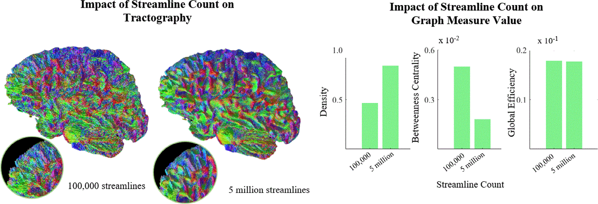
Visually, streamline count does not clearly impact perception of tractography (left), which may lead one to think that they are equivalent. Given these tractography data, we can represent the human connectome as an adjacency matrix and compute graph-based measures to assess connectivity. Common measures on the data presented at left such as density, betweenness centrality, and global efficiency show substantial and varied dependence on streamline count (right).

Herein, this article investigated the relationship between streamline count and 13 graph theory measures. Specifically, graph measures were assessed for repeatability, reproducibility, and convergence to a reference mean.

Materials and Methods

The data acquisition was approved by Cardiff University ethics committee. Written informed consent was obtained from all subjects.

As summarized in Fig. 2, subjects from a previous DWI-MRI cohort were preprocessed using MRtrix (version 3.0.0; https://www.mrtrix.org).¹¹ Then, MRtrix anatomically informed tractography was performed using MRtrix.¹² For each dataset, the number of streamlines used was varied from 1 × 10² to 5 × 10⁷. The 5 × 10⁷ streamlines is an extreme over-estimate of current practice.¹¹ For each tractogram, streamlines were mapped to representative adjacency matrices called connectomes.¹³ Connectomes were then analyzed with graph-theory measures.^6,14 With this experimental design, we assessed how graph-theory measure reproducibility is impacted by the number of streamlines used during tractography. QIBA Technical Performance Working Group provide definitions for repeatability and reproducibility; repeatability is variability of the metric “when repeated measurements are acquired on the same experimental unit under identical or nearly identical conditions” and reproducibility is “associated with using the imaging instrument in real world clinical settings which are subject to a variety of external factors that cannot all be tightly controlled.”¹³ ICC is a measure of repeatability that quantifies the consistency of a repeated measure relative to the total population variation.^13,14 CCC is measure of reproducibility that evaluates the agreement between multiple observations per experiment without ANOVA assumptions.^13,15 To test whether a graph measure is dependent on streamline count, we assess whether the measure converges to the mean value computed at 50 million streamlines regions (as indicated by “reference”). Fifty million streamlines are 10-fold larger than streamline counts used in the literature.¹² For evaluation, a paired t-test compares the mean value at streamline count, s, to the mean value at the reference.¹⁶

FIGURE 2:

We generated 5000 tractography files. Tractography files were converted to matrices using MRTrix tck2connectome command, resulting in 5000 connectomes that span 10 subjects and 50 streamline counts. We assessed connectome connectivity with global and nodal graph-based measures. Each global graph-measure resulted in a single value per connectome and nodal measures were averaged across nodes for a total of 13 measures.

Data Acquisition

The dataset consisted of 10 de-identified subjects from the Multi-shell Diffusion MRI Harmonization Challenge 2018 (MUSHAC) dataset.¹⁵ Demographic information is as follows: all healthy, 70% female, and with age range of 25.3 ± 5.9 years. Structural T1-weighted and DWI data were acquired with a 3-Tesla Siemens Connectom scanner (Siemens Healthineers, Erlangen, Germany) with the same acquisition protocol across subjects, respectively. The diffusion pulse spin echo sequence had the following parameters: echo time (TE) = 68 msec, repetition time (TR) = 5.4 seconds, 120 slices, and field of view = 188 mm². Voxels had an isotropic resolution of 1.2 mm³. The DWI data were acquired with two gradient strengths (b-values = 1200 and 3000 sec/mm²) and shell samples = 60, 60. Eighteen images without diffusion weighting were also acquired (b0, b = 0 sec/mm²).

Preprocessing

Each subject was corrected for eddy current distortions, motion, echoplanar imaging (EPI) distortions, and gradient-nonlinearity distortions using FSL TOPUP/eddy (version 3.0.3; https://fsl.fmrib.ox.ac.uk/fsl/fslwiki)¹⁶ from the Human Connectome Project (HCP) minimal preprocessing pipeline.¹⁷ The minimally weighted (b0) volumes were corrected for EPI distortions on phase-encoding pairs also using FSL TOPUP.

To prepare the DWI data for tractography, we performed the default MRTrix processing pipeline (version 5.0.10; https://www.mrtrix.org).¹¹ First, used was dwi2response with the Dhollander algorithm to estimate response functions for grey matter (GM), WM, and cerebrospinal fluid (CSF) compartments.¹⁸ The Dhollander algorithm offers an unsupervised estimation of WM, GM, and CSF response functions with multishell multi-tissue constrained spherical deconvolution (CSD).¹¹ Further, dwi2fod uses these response functions to generate fiber orientation distributions (FODs). This process used multishell multitissue CSD to generate spherical harmonic coefficients.¹⁹ Seeding was limited to anatomically plausible locations with a five-tissue-type segmented tissue image for input to anatomically constrained tractography (ACT).¹²

Tractography

Ten tractograms with 50 million streamlines were created with the tckgen command for each subject.¹¹ MRTirx default probabilistic tracking algorithm of second-order integration over fiber orientation distributions (iFOD2) was used for tractography.²⁰ These streamlines were randomly sampled without replacement each 50 million streamline tractogram to compute streamline counts from 1 × 10² to 5 × 10⁷. The number of streamlines that result from this sampling is defined as “streamline count.” Tractography seeding and termination was constrained using the five-tissue-type mask, and we allowed backtracking.

Connectomics

tck2connectome maps streamlines to an adjacency matrix based on their termination locations.¹³ The bundles were defined by the Desikan-Killiany atlas²¹ from Freesurfer (version 7.2.0; https://surfer.nmr.mgh.harvard.edu) with 87 cortical and subcortical regions²² In this article, there are two connectomes on this node structure. First, edge weight reflects the number of streamlines connecting two brain regions (as indicated by “connectome weighted by number of streamlines”). Second, the edge weight reflects the average streamline length in millimeters connecting two brain regions (as indicated by “connectome weighted by mean length of streamlines”). Note, as streamline count increases, the streamlines used for both metrics increases. Small-worldness, randomness, characteristic path length, and average betweenness centrality used the connectome weighted by mean length of streamlines. Modularity, global efficiency, assortativity, density, edge count, average participation coefficient, average local efficiency, average node strength, average clustering coefficient, and average betweenness centrality used the connectome weighted by number of streamlines. In total, this experimental design resulted in 5000 connectomes from 10 subjects, 50 streamline counts, and 10 repeats.

Table 1 details additional graph-measure specific alterations to the connectomes. Global efficiency, local efficiency, and clustering coefficient required normalization and density required binarization. Randomness and small-worldness cannot be computed on sparse connectomes and is often represented as inf. These inf values were filtered out and replaced with NaN to be compatible with downstream methods could not handle such data representations. Average and standard deviation calculations ignored NaN values.

TABLE 1.

Connectome Preprocessing

Graph Measure	Edge Weight		Preprocessing
	Number of Streamlines	Mean Length	Threshold	Normalize	Binarize	Remove NaN/∞
Modularity	X
Global efficiency	X			X
Assortativity	X
Density	X				X
Density with adaptive thresholding	X		X		X
Edge count	X					X
Characteristic path length		X
Small-worldness		X				X
Randomness		X				X
Average participation coefficient	X
Average local efficiency	X			X
Average local efficiency with adaptive thresholding	X		X	X
Average node strength	X
Average normalized node strength	X			X
Average node degree	X
Average normalized node degree	X			X
Average clustering coefficient	X			X		X
Average clustering coefficient with adaptive thresholding	X		X	X		X
Average betweenness centrality		X

Detailed here are the edge weight and preprocessing steps associated with each graph measure. Each connectome is preprocessed with BCT. Density, local efficiency, node strength, and clustering coefficient have alternate versions in which additional preprocessing is applied. We offer alternative definitions that converge to an unbiased estimate, where the original definitions do not.

For measures that did not converge to an unbiased estimate or did not achieve the desired correlations, d variations to ensure convergence (normalization, adaptive thresholding) are provided. Adaptive thresholding used the underlying probability distribution of the connectome to decrease the effect of false-positive streamlines on graph measure value. An edge must have more than 10⁻⁵% of the total number of streamlines in the connectome to be considered in graph measure calculations.

Graph Measures

The Brain Connectivity Toolbox (BCT) (version March 03, 2019) is a Matlab-based toolbox for complex network analysis.⁶ This included all but three (randomness, small-worldness, and edge count) graph measures in Table 1. Randomness, small-worldness, and edge count are defined in the BCTpy toolbox, a Python-based extension of the original toolbox.¹⁴

The BCT and BCTpy definitions used for each graph measure are as follows ^6,19 Note that nodal measures were calculated for all nodes and averaged together. Modularity is the degree to which the network may be subdivided into clearly delineated and nonoverlapping groups.⁶ Let $m_i$ be the module containing node $i,w_{ij}$ be the weight of connection between nodes $i$ and $j,k_i^w$ is the weighted degree of node $i$, and $l^w$ is the weighted sum of all nodes in the connectome.

$$\begin{array}{l}\frac{1}{l^w}{\sum }_{i,j\in N}\left(w_{ij}-\left(\frac{k_i^w{k}_j^w}{l^w}\right)\right){\delta }_{m_i,m_j,}{\delta }_{m_i,m_j}\\ =\{\begin{array}{ll}1,m_i=m_j\hfill & \hfill \\ \hfill & 0,m_i\ne m_j\hfill \end{array}\end{array}$$

Global efficiency is the average inverse shortest path length. Let be $d_{ij}$ the shorted path length between nodes $i$ and $j$.⁶

$$\frac{1}{n}{\sum }_{i\in N}\frac{{\sum }_{j\in N,j\ne i}{\text{d}}_{ij}^{-1}}{n-1}$$

Assortativity is a correlation coefficient between the degrees of all nodes on two opposite ends of a link and represents resilience.⁶

$$\frac{l^{-1}{\sum }_{(i,j)\in L}{w}_{ij}{k}_i^w{k}_j^w-{\left[l^{-1}{\sum }_{(i,j)\in \text{L}}\frac{1}{2}{w}_{ij}(k_i^w+k_j^w)\right]}^2}{[l^{-1}{\sum }_{(i,j)\in L}\frac{1}{2}{w}_{ij}({(k_i^w)}^2+{(k_j^w)}^2)]-{\left[l^{-1}{\sum }_{(i,j)\in L}\frac{1}{2}{w}_{ij}(k_i^w+k_j^w)\right]}^2}$$

Density is the fraction of present connections to the possible connections ⁶

$$\frac{{\sum }_{i\in N}{\sum }_{j\in N}{a}_{ij}}{\frac{N^2-N}{2}}$$

Edge count is the number of edges in the characteristic path length.¹⁹ The characteristic path length is the average shortest path between nodes in millimeters.⁶

$$\frac{1}{n}{\sum }_{i\in N}\frac{{\sum }_{j\in N,j\ne i}{d}_{ij}^w}{n-1}$$

Small-worldness defines whether a network is considered smallworld.¹⁹ Randomness defines if a network has random or lattice-like structure.¹⁹ Randomness ranges between −1 and 1, where a value close to 0 means the connectome has small-world characteristics, values close to −1 mean that network has a lattice structure, and values close to 1 mean the network is random. Local efficiency is global efficiency calculated on the neighborhood of a node.⁶

$$\frac{1}{2}{\sum }_{i\in N}\frac{{\left({\sum }_{j,\mathrm{h}\in N,j\ne i}{w}_{ij}{w}_{ih}{\left[d_{ijh}\left(N_i\right)\right]}^{-1}\right)}^{\frac{1}{3}}}{k_i\left(k_i-1\right)}$$

Node strength is the sum of weights of links connected to a node.⁶

$${\sum }_{j\in N}{w}_{ij}$$

Node degree is the total number of nodes connected to a given node.⁶ The clustering coefficient is the geometric mean of all triangles associated with a node.⁶ Let $t_i=\frac{1}{2}{\sum }_{j,h\in N}{a}_{ij}{a}_{ih}{a}_{jh}$ be the number of triangles around node $i$.

$$\frac{2t_i^w}{k_i\left(k_i-1\right)}$$

Betweenness centrality is the fraction of shortest paths in the network that contain a given node.⁶

$$\frac{1}{(n-1)(n-2)}\sum _{h,j\subset N,h\ne j,h\ne i,j\ne i}\frac{{\rho }_{hj}(i)}{{\rho }_{hj}}$$

where ${\rho }_{hj}$ is the number of shortest paths between $h$ and $j$, and ${\rho }_{hj}(i)$ is the number of shortest paths between $h$ and $j$ that pass through. The participation coefficient is the diversity of intermodular connections of individual nodes.⁶

$$1-{\sum }_{m\in M}{\left(\frac{k_i(m)}{k_i}\right)}^2$$

where $M$ is the set of modules and $k_i(m)$ is the number of edges between $i$ and all nodes in the module $m$.

Statistical Analysis

For statistical analyses, Matlab software (version 3.0.3; The MathWorks Inc., Natick, MA, USA) was used. The following statistical tests were performed to quantify the repeatability and reproducibility of each graph measure and to assess its dependence on streamline count. A measure has dependence on streamline count if it is unable to converge to an unbiased reference estimate as streamline count increases. Tractography generated with 5 × 10⁷ streamlines is more than sufficient and, thus, these tests aimed to identify tractography with less streamlines that has the same properties (average value, ICC, CCC).¹²

Convergence to an unbiased estimate was assessed using two-sample t-tests with 5% confidence.²³ The null hypothesis was that the data at a given streamline count and the data at a streamline count of 50 million came from independent random samples from normal distributions with equal means and unequal variances. The alternative hypothesis was that the two data came from populations with unequal means. This test indicated whether a similar distribution was achieved at a smaller streamline count than 50 million. The t-test was computed between the 10 pairs of subjects each with 10 repeated experiments at a given streamline count, s, and 50 million streamlines. Due to the graph measures having unique scales and standard deviations, additional power analysis was performed for each measure separately. The parameters and results of all power analyses can be found in Table S1 in the Supplemental Material.

The ICC quantified how well measurements of the same group resembled each other. QIBA Technical Performance Working Group suggests using ICC to evaluate repeatability. There are two established interpretations according to Cicchetti²⁴ and Koo and Li²⁵ that classified data as excellent, good, or poor/moderate according to intragroup resemblance and intergroup distinction. The ICC ranges for each category were defined as follows: Koo and Li defined ICC below 0.5 as “poor,” between 0.50 and 0.75 as “moderate,” between 0.75 and 0.90 as “good,” and above 0.90 as “excellent.”²⁵ This test assesses whether graph measures from the same subject, but different tractography generations had similar values and if graph measures from different subjects were statistically distinguishable. A P value <0.05 was considered statistically significant.

The QIBA Technical Performance Working Group suggests using CCC to evaluate the reproducibility of quantitative metrics.¹³ CCC evaluates the agreement between multiple observations and quantifies the extent to which paired measurements differ from perfect agreement. CCC value is interpreted as follows: above 0.99 as “almost perfect,” from 0.95 to 0.99 as “substantial,” 0.90 to 0.95 as “moderate,” and less than 0.90 as “poor” (31).

Results

Streamline count invariance is assessed with three benchmarks: convergence to a reference mean, excellent repeatability, and almost perfect reproducibility. The streamline counts that each graph measure achieved these benchmarks are recorded in Table 2. In Fig. 3, the streamline count at which the data converge to the reference mean is represented with a black vertical line. Data at streamline counts greater than this have converged and no longer increase or decrease as streamline count changes. Figures 4 and 5 have two types of measures: original definitions and alternate definitions. None of these original definitions converged to their unbiased reference mean. Proposed alternate definitions that do converge are included with new convergence points are marked with a black vertical line.

TABLE 2.

Summary Table of Results

Graph Measure	Streamline Count of First Convergence to Reference Mean	Streamline Count When First Reached ICC > 0.9	Streamline Count When First Reached CCC > 0.99
Modularity	1.24 E + 04	1.38 E + 05	5.87 E + 06
Global efficiency	4.73 E + 04	9.49 E + 03	6.18 E + 04
Edge count	1.38 E + 05	7.67 E + 06	-
Small worldness	8.08 E + 04	1.00 E + 07	-
Randomness	3.62 E + 04	1.00 E + 07	-
Average betweenness centrality	1.38 E + 05	7.67 E + 06	-
Average participation coefficient	5.55 E + 03	-	-
Assortativity	2.49 E + 03	-	-
Density	-	1.24 E + 04	5.27 E + 05
Density with adaptive thresholding	5.87 E + 06	1.24 E + 04	3.08 E + 05
Characteristic path length	-	2.01 E + 06	2.93 E + 07
Characteristic path length with adaptive thresholding	2.49 E + 03	2.01 E + 06	-
Average node degree	-	1.24 E + 04	5.27 E + 05
Average node degree with adaptive thresholding	5.87 E + 06	1.24 E + 04	3.08 E + 05
Average node strength	-	3.62 E + 04	3.08 E + 05
Average normalized node strength	1.62 E + 04	9.49 E + 03	1.81 E + 05
Average local efficiency	-	1.24 E + 04	1.38 E + 05
Average local efficiency with adaptive threshold	2.01 E + 06	1.24 E + 04	3.08 E + 05
Average clustering coefficient	-	1.24 E + 04	1.81 E + 05
Average clustering coefficient with adaptive thresholding	2.36 E + 05	1.24 E + 04	3.08 E + 05

The number of streamlines needed to converge to a reference mean (column 2), achieve excellent repeatability (column 3), and achieve almost perfect reproducibility (column 4). A “-” reflects that a measure did not converge, or reach ICC > 0.9 or CCC > 0.99 with less than 50 million streamlines.

FIGURE 3:

Each subject is represented by a different color with its mean and range of one standard deviation. As streamline count increases the change in mean value plateaus. The black vertical line marks when the distance between means of a streamline count and the reference is approximately zero.

FIGURE 4:

Density, average node strength, average node degree, average local efficiency, and average clustering coefficient continue to change with increasing streamline count. We conclude that these measures are dependent on streamline count. The black vertical line marks when the distance between means of a streamline count and the reference is approximately zero. None of these measures achieve that. We provide alternate definitions that do. Average node strength converges when normalized. With adaptive thresholding, the remaining measures converge.

FIGURE 5:

ICC (blue) and CCC (red) for six streamline counts 1E2 to 5E7.

Repeatability was measured with ICC. Modularity, global efficiency, edge count, characteristic path length, small-worldness, randomness, average betweenness centrality, density, average node strength, average node degree, average local efficiency, and average clustering coefficient had excellent repeatability (ICC > 0.90) at of before a streamline count of 10 million (Fig. 5). Assortativity and average participation coefficient only had good repeatability at the highest streamline counts tested (50 million streamlines).

Figure 5 shows reproducibility test results from CCC in blue. Modularity, global efficiency, edge count, characteristic path length, density, average node strength, average node degree, average local efficiency, and average clustering coefficient, had almost perfect reproducibility (CCC > 0.99) at or before 10 million streamlines. Edge count, small-worldness, randomness, and average betweenness centrality only reached substantial reproducibility (CCC > 0.95) at the highest streamline counts tested. Assortativity and average participation coefficient only reached moderate reproducibility (CCC > 0.90) at the highest streamline counts tested.

Discussion

We found a variety of relationships between streamline count and graph measure value, repeatability, and reproducibility. Streamline count invariant graph measures will be comparable across streamline counts, be reproducible, and repeatable. To be comparable across streamline counts, the mean value should not change past a certain point. Modularity and global efficiency had lowest dependency on streamline count: both converged, had excellent repeatability, and almost perfect reproducibility for streamline counts greater than 6 million and 100,000 streamlines, respectively. Density and average node strength were strongly dependent on streamline count and therefore their values were only comparable when using the same number of streamlines during tractography. Based on our findings, we recommend using an alternative definition with adaptive thresholding or normalization, respectively, which makes their values comparable past a certain streamline count. While it is not considered common practice, we encourage future studies to include streamline counts in their technical details to ensure valid comparisons across experiments. The storage and computational burden of tractography is highly dependent on streamline count and, therefore, it is important to avoid overestimations.

Previous literature characterized the relationship between streamline counts and reproducibility of diffusion-related measures for certain tractography variations but not its impact on graph theory analysis specifically (26, 27). Yeh et al investigated the streamline count required for reproducible connectome reconstructions across parcellation resolutions.²⁶ They found that parcellations with ~200 nodes could achieve “acceptable reproducibility” (coefficient of variation of 0.1), but parcellation larger parcellation schemes with more than 400 nodes needed more streamlines to achieve the same reproducibility. The experimental design was limited to a maximum of 5 million streamlines. In this article, we only considered one parcellation resolution (87 regions) but a wider range of streamline counts. Moreover, Reid et al explored the number of streamlines needed for reliable when performing probabilistic tractography.²⁷ They focused on the impact of number of streamlines on fractional anisotropy and mean diffusivity reproducibility. In this article, we also used probabilistic tracking but chose to investigate how this recommendation changes based on other metrics of interest: graph measures.

Limitations

The small sample size and demographic makeup of this study is a major limitation. Future work should expand these tests for a greater number of patients (healthy, impaired, male, female, and ages). Furthermore, in this study, we did not consider other tractography variations such as probabilistic versus deterministic algorithms, voxel resolution, seeding settings, or parcellation resolutions, nor did we investigate how acquisition parameters and quality would affect these parameters. We believe that these variations may have substantial influence on the graph measures and their ability to be compared.

Conclusion

Modularity and global efficiency were streamline count invariant in terms of mean value, repeatability, and reproducibly. At 10 million streamlines, both had excellent repeatability and nearly perfect reproducibility. Density, average node strength, average node degree, characteristic path length, average local efficiency, and average clustering coefficient were dependent on streamline count and therefore their values were only comparable when using the same number of streamlines during tractography or when using the alternate definitions. Remaining measures had low dependency on streamline count.

Data Availability Statement

Multi-shell Diffusion MRI Harmonization Challenge 2018 (MUSHAC) is a publicly available dataset. The data acquisition was approved by Cardiff University School of Psychology ethics committee. The code used for this article is available from the corresponding author on reasonable request.

References

- 1.Essayed WI, Zhang F, Unadkat P, Cosgrove GR, Golby AJ, O’Donnell LJ. White matter tractography for neurosurgical planning: A topography-based review of the current state of the art. Neuroimage Clin 2017;15:659–672. [DOI] [PMC free article] [PubMed] [Google Scholar]
- 2.Mori S, van Zijl PCM. Fiber tracking: Principles and strategies - a technical review. NMR Biomed 2002;15:468–480. [DOI] [PubMed] [Google Scholar]
- 3.Zhang J, Richards LJ, Yarowsky P, Huang H, van Zijl PCM, Mori S. Three-dimensional anatomical characterization of the developing mouse brain by diffusion tensor microimaging. Neuroimage 2003;20:1639–1648. [DOI] [PubMed] [Google Scholar]
- 4.Conturo TE, Lori NF, Cull TS, et al. Tracking neuronal fiber pathways in the living human brain. Appl Phys Sci 1999;96:10422–10427. [DOI] [PMC free article] [PubMed] [Google Scholar]
- 5.Bullmore E, Sporns O. Complex brain networks: Graph theoretical analysis of structural and functional systems. Nat Rev Neurosci 2009;10:186–198. [DOI] [PubMed] [Google Scholar]
- 6.Rubinov M, Sporns O. Complex network measures of brain connectivity: Uses and interpretations. Neuroimage 2010;52:1059–1069. [DOI] [PubMed] [Google Scholar]
- 7.Yuan W, Wade SL, Babcock L. Structural connectivity abnormality in children with acute mild traumatic brain injury using graph theoretical analysis. Hum Brain Mapp 2014;36(2):779–792. [DOI] [PMC free article] [PubMed] [Google Scholar]
- 8.Daianu M, Jahanshad N, Nir TM, et al. Breakdown of brain connectivity between normal aging and Alzheimer’s disease: A structural k-core network analysis. Brain Connect 2013;3(4):407–422. [DOI] [PMC free article] [PubMed] [Google Scholar]
- 9.Bernhardt BC, Chen Z, He Y, Evans AC, Bernasconi N. Graphtheoretical analysis reveals disrupted small-world organization of cortical thickness correlation networks in temporal lobe epilepsy. Cereb Cortex 2011;21:2147–2157. [DOI] [PubMed] [Google Scholar]
- 10.Dennis EL, Jahanshad N, Toga AW, et al. Changes IN anatomical BRAIN connectivity between ages 12 and 30: A HARDI study of 467 adolescents and adults. Proceedings of the IEEE international symposium on biomedical imaging: From nano to macro IEEE international symposium on biomedical imaging, Vol 904: IEEE; 2012. [DOI] [PMC free article] [PubMed] [Google Scholar]
- 11.Tournier JD, Smith R, Raffelt D, et al. MRtrix3: A fast, flexible and open software framework for medical image processing and visualisation. Neuroimage 2019;202:116137. [DOI] [PubMed] [Google Scholar]
- 12.Smith RE, Tournier JD, Calamante F, Connelly A. Anatomically-constrained tractography: Improved diffusion MRI streamlines tractography through effective use of anatomical information. Neuroimage 2012;62:1924–1938. [DOI] [PubMed] [Google Scholar]
- 13.Smith RE, Tournier JD, Calamante F, Connelly A. The effects of SIFT on the reproducibility and biological accuracy of the structural connectome. Neuroimage 2015;104:253–265. [DOI] [PubMed] [Google Scholar]
- 14.bctpy PyPI https://pypi.org/project/bctpy/.
- 15.Challenge Multi-shell diffusion MRI harmonisation challenge 2018 (MUSHAC) https://projects.iq.harvard.edu/cdmri2018/challenge.
- 16.Jenkinson M, Beckmann CF, Behrens TEJ, Woolrich MW, Smith SM. FSL. Neuroimage 2012;62:782–790. [DOI] [PubMed] [Google Scholar]
- 17.Glasser MF, Sotiropoulos SN, Wilson JA, et al. The minimal preprocessing pipelines for the human connectome project. Neuroimage 2013;80:105–124. [DOI] [PMC free article] [PubMed] [Google Scholar]
- 18.(PDF) Unsupervised 3-tissue response function estimation from single-shell or multi-shell diffusion MR data without a co-registered T1 image. https://www.researchgate.net/publication/307863133_Unsupervised_3-tissue_response_function_estimation_from_single-shell_or_multi-shell_diffusion_MR_data_without_a_co-registered_T1_image.
- 19.Jeurissen B, Tournier JD, Dhollander T, Connelly A, Sijbers J. Multi-tissue constrained spherical deconvolution for improved analysis of multi-shell diffusion MRI data. Neuroimage 2014;103:411–426. [DOI] [PubMed] [Google Scholar]
- 20.ISMRM 2010. Improved probabilistic streamlines tractography by 2nd order integration over fibre orientation distributions https://archive.ismrm.org/2010/1670.html
- 21.Klein A, Tourville J. 101 labeled brain images and a consistent human cortical labeling protocol. Front Neurosci 2012;6:171. [DOI] [PMC free article] [PubMed] [Google Scholar]
- 22.CorticalParcellation Free Surfer Wiki. https://surfer.nmr.mgh.harvard.edu/fswiki/CorticalParcellation.
- 23.Two-sample t-test - MATLAB ttest2. https://www.mathworks.com/help/stats/ttest2.html.
- 24.Guidelines Cicchetti D., criteria, and rules of thumb for evaluating normed and standardized assessment instruments in psychology. Psychol Assess 1994;6:284–290. [Google Scholar]
- 25.Koo TK, Li MY. A guideline of selecting and reporting intraclass correlation coefficients for reliability research. J Chiropr Med 2016;15:155–163. [DOI] [PMC free article] [PubMed] [Google Scholar]
- 26.Yeh C-H, Smith R, Liang X, Calamante F, Connelly A. Investigating the streamline count required for reproducible structural connectome construction across a range of brain parcellation resolutions. 1558: Proceedings of ISMRM, June 2018. [Google Scholar]
- 27.Reid LB, Cespedes MI, Pannek K. How many streamlines are required for reliable probabilistic tractography? Solutions for microstructural measurements and neurosurgical planning. Neuroimage 2020;211:116646. [DOI] [PubMed] [Google Scholar]
Associated Data
This section collects any data citations, data availability statements, or supplementary materials included in this article.
Supplementary Materials