

Highlights
-
•
Active power in sonoreactors can vary by a factor 2 depending on immersion depth.
-
•
Some luminol maps in sonoreactors are reminiscent of linear acoustics eigenmodes.
-
•
Luminol maps in sonoreactors reveal elongated bright zones above some threshold.
-
•
The geometry of sonoreactors strongly influence cavitation zones.
-
•
Comparison of luminol maps with non-linear full model of sonoreactors partially fails.
Keywords: Ultrasound, Acoustic cavitation, Simulation, Sono-chemiluminescense, Calorimetry
Abstract
This investigation focuses on the influence of geometric factors on cavitational activity within a 20kHz sonoreactor containing water. Three vessels with different shapes were used, and the transducer immersion depth and liquid height were varied, resulting in a total of 126 experiments conducted under constant driving current. For each one, the dissipated power was quantified using calorimetry, while luminol mapping was employed to identify the shape and location of cavitation zones. The raw images of blueish light emission were transformed into false colors and corrected to compensate for refraction by the water–glass and glass-air interfaces. Additionally, all configurations were simulated using a sonoreactor model that incorporates a nonlinear propagation of acoustic waves in cavitating liquids. A systematic visual comparison between luminol maps and color-plots displaying the computed bubble collapse temperature in bubbly regions was conducted. The calorimetric power exhibited a nearly constant yield of approximately 70% across all experiments, thus validating the transducer command strategy. However, the numerical predictions consistently overestimated the electrical and calorimetric powers by a factor of roughly 2, indicating an overestimation of dissipation in the cavitating liquid model. Geometric variations revealed non-monotonic relationships between transducer immersion depth and dissipated power, emphasizing the importance of geometric effects in sonoreactor. Complex features were revealed by luminol maps, exhibiting appearance, disappearance, and merging of different luminol zones. In certain parametric regions, the luminol bright regions are reminiscent of linear eigenmodes of the water/vessel system. In the complementary parametric space, these structures either combine with, or are obliterated by typical elongated axial structures. The latter were found to coincide with an increased calorimetric power, and are conjectured to result from a strong cavitation field beneath the transducer producing acoustic streaming. Similar methods were applied to an additional set of 57 experiments conducted under constant geometry but with varying current, and suggested that the transition to elongated structures occurs above some amplitude threshold. While the model partially reproduced some experimental observations, further refinement is required to accurately account for the intricate acoustic phenomena involved.
1. Introduction
Ultrasound has been used in several applications in Chemical and Process Engineering, covering solid–liquid processes, such as effluent treatment [1], [2], extraction [3], aggregation [4], [5], dispersion [6], [7] and crystallization [8], [9], [10], liquid–liquid process (emulsification [11], [12]), gas–liquid process (atomization [13], [14], [15]), and also in various reaction processes, such as polymerization [16], [17], hydrogen production [18], [19], [20] and sonochemistry [21], [22], [23], [24]. The chemical and physical effects of ultrasound sought in all these processes are linked to the phenomenon of acoustic cavitation [25]: millions of micro-bubbles of gas appear in the liquid under the influence of pressure changes caused by the acoustic wave, and then collapse very violently resulting in a huge concentration of energy (few hundred atmospheres pressure and few thousand Kelvin temperature in the bubbles).
Despite its potential for industrial use [26], [27], [28], most sonochemical effects are studied at the laboratory scale. The challenge of designing cavitational reactors on an industrial scale is related to many problems, including the lack of precise quantification of the bubbles location and dynamic behaviour according to different operating and geometric conditions, the absence of appropriate design strategies connecting the theoretically available information (bubble dynamics) with the experimental results, and the unavailability of a trustworthy tool available to predict and design sonochemical reactors. This is due, in part, to the extreme physical complexity of acoustic cavitation, which renders dimensional analysis impractical. Furthermore, since ultrasound is employed, acoustics should be one of the most important aspects to be considered in sonoreactors science, but remains one of the most overlooked in previous studies.
In recent years, there has been a growing interest in computational approaches to predict the behaviour of sonoreactors, to circumvent the difficulty in their scale-up. The performance of these reactors depends on many parameters, such as geometry, transducer design, frequency operation, intensity and propagation medium [29]. A recent example features a study by Rashwan and co-workers [30] who used acoustic pressure field simulations to optimise the mechanical and geometrical designs of a sonoreactor for hydrogen production. Several groups [31], [32], [33], [34] have used numerical models based on the linearised version of the Caflisch model [35] developed by Commander & Prosperetti [36]. As the latter assumes linear oscillations of the bubbles, this method produces largely underestimated attenuation coefficients when inertial cavitation is present [37].
The major dissipators in the liquid are the bubbles and the power measured by calorimetric approach results from the mechanical power that each bubble converts into heat. Most studies stated above are unable to compute the calorimetric power accurately, either because bubbles are completely ignored, or because an underlying assumption of linear oscillations leads to a significant underestimation of the energy they dissipate [38]. Based on Caflisch’s model and taking into consideration fully nonlinear bubble dynamics, Louisnard developed a modified non-linear model of sound propagation in cavitating liquids to get rid of the latter restriction [39], [40]. Calculating the power dissipated by bubbles under this model becomes simple since the suggested non-linear Helmholtz equation directly incorporates the latter. The ability of this model has been enhanced by coupling the pressure field in the liquid with the elastic vibrations of both the solid walls [41] and the transducer [42]. The modelling of the latter has become easy thanks to the implementation of piezo-electricity equations in most finite elements codes, among others COMSOL Multiphysics. Therefore, as shown by Garcia-Vargas et al. [43], modeling a complete sonoreactor becomes feasible as far as the internal design of the transducer is precisely known. This extensive modelling allows to restrict the inputs of the model to the experimentally controllable ones: frequency and driving current. The additional difficulty brought by the automatic frequency selection implemented on modern ultrasonic generators can also be addressed in simulations, as shown recently in Refs [43], [42].
Sonoreactor models should be effectively tested by examining their predictive capability when geometry and operational parameters are varied parametrically. A first attempt in this way was performed in a precedent study where the global electrical quantities predicted by our model was bluntly compared to their experimental counterparts monitored by the generator [43]. Although the orders of magnitude of our predictions were within the correct range and some tendencies could be caught, some discrepancies were observed, particularly for geometric effects, and some yet unidentified acoustic effects were called into question. To elucidate the latter aspects, a closer comparison between our predicted pressure fields and an experimental characterization of the latter was necessary.
Sono-chemiluminescence (SCL) is one of the most used qualitative experimental methods, as it allows a direct observation of cavitation zones within a reactor [44], [45], [46], [47], [48], [49]. It consists in recording the bright emission of luminol chemiluminescence in a water alkaline solution irradiated by ultrasound. Renaudin et al. [46] studied the sonochemical luminescence intensity at high frequency (500kHz) in function of liquid height, and showed that the effects of sonochemical reactions decreased as liquid height was increased. Son et al. [50] investigated several parameters (sonotrode immersion depth, electrical input power, liquid height, horizontal position of the probe, and thickness of the bottom plate) to optimize a system consisting of a 20kHz sonotrode immersed in a 500ml glass beaker using several characterization methods, including SCL. Using the same technique, Lee and co-workers [51] were able to analyse the influence of liquid re-circulation under different liquid heights ranging from 1 to 4 wavelengths and flow rates from 1.5 to 6.0 L min−1, respectively.
The SCL method can be also used in heterogeneous systems containing liquid and solid phases [52], [53]. Recently, Choi & Son [54] studied a system composed of a 20kHz sonotrode immersed in a homogeneous and heterogeneous medium consisting of water and glass beads. The authors showed that for the homogeneous system, the glowing zones were concentrated near the tip of the sonotrode. Conversely, for the heterogeneous system, active zones appeared in almost all the vessel, and light intensity was mostly uniform. Barchouchi [55] also studied the influence of glass beads on the luminol emission at low and high frequency. The results obtained by SCL showed a uniform spatial distribution over a large range of specific surface areas.
Simulating experimental results reported in the literature is often difficult mainly because precise data on the vessel and/or transducer geometry are lacking. The purpose of this study is to map the cavitational activity of the well documented 20kHz sonoreactors by SCL, in a large range of experimental conditions, including the liquid height, the transducer immersion depth, and the input current amplitude, which is the quantity experimentally controlled by the generator level button. For each experimental configuration, a calorimetric measurement is also performed and all electrical data are monitored. Finally, each configuration is also simulated with our model and systematically compared to luminol maps (183 in total), after a careful correction of image aberrations due to the vessel curvature. Results of KI oxidation experiments under the same conditions will be presented in a future paper.
2. Material and methods
2.1. Chemicals
Luminol (3- aminophthalhydrazide, 98%) from Alfa Aesar and sodium hydroxide (> 97%) from Fisher Chemicals were used as received without additional purification. All solutions were prepared from distilled water at ambient temperature.
2.2. Experimental setup
The experimental setup is similar to the one reported in Ref. [43] and is displayed in Fig. 1. Acoustic cavitation was produced by a transducer immersed in the center of three different commercial glass vessels (hereinafter referred to as A, B and C) filled with tap water. Table 1 shows the dimensions of the vessels.
Fig. 1.

Schematic of the experimental setup.
Table 1.
Geometrical characteristics of the beakers (see Fig. 1).
| Vessel | Form | Capacity (L) | (mm) | H (mm) | d (mm) |
|---|---|---|---|---|---|
| A | wide | 1.0 | 106 | 143 | 23 |
| B | narrow | 2.0 | 120 | 237 | 25 |
| C | wide | 2.0 | 132 | 183 | 22 |
The transducer used in this study was a 20kHz homemade standard Langevin-type (SinapTec, Lezennes, France) with two piezoelectric rings pre-stressed by a steel screw between a mass and counter-mass, both made of titanium alloy. Using an impedance-bridge, the precise resonance frequency of the unloaded transducer, , was determined. A computer-controlled ultrasonic generator (SinapTec NexTgen Inside 500) was used to drive the transducer with a controlled input-current and an automatic frequency control ensuring a purely resistive motionnal branch (see Refs [43], [42] for details). During experiments, various electrical quantities can be monitored and logged every 50ms: frequency, voltage and current as well their mutual phase, impedance, and active electrical power. In order to monitor the temperature increase throughout the experiments, a PT100 probe was additionally connected to the ultrasonic generator and temperature was monitored along with the electrical quantities. The transducer was submerged in each of the three glass vessels, and two geometrical parameters could be varied: the distance between the transducer’s tip and the vessel’s bottom and the water level . The transducer immersion depth can be deduced from the latter.
In this study, three sets of experiments were carried out (see summary in Table 2). In the first set, the input current of the transducer was fixed at a constant value of and was swept in a vessel-dependent range at constant liquid volume . Thus, the liquid level varied in function of the bottom-transducer distance , in such a way that:
| (1) |
where is the vessel internal diameter and is the transducer diameter (). Thus, an initial configuration , the liquid height is deduced from by:
| (2) |
Table 2.
Summary of parameters used in experiments.
| Experiment set | Vessel | (mm) | (mm) | (A) | ||
|---|---|---|---|---|---|---|
| Set 1 | (mm) | (mm) | ||||
| A | 20 | 120 | 20 to 100 | Computed from Eq. (2) | 0.6 | |
| B | 80 | 190 | 80 to 170 | |||
| C | 30 | 150 | 30 to 130 | |||
| Set 2 | A | 20 | 30 to 130 | 0.6 | ||
| B | 80 | 90 to 200 | ||||
| C | 30 | 40 to 160 | ||||
| Set 3 | A | 60 | 113 | 0.08 to 0.8 | ||
| B | 110 | 186 | ||||
| C | 80 | 145 |
In the second set, the liquid height was varied and the position of the transducer inside the vessel was fixed at for the vessel A, for the vessel B and for the vessel C, in order to allow a largest range for in each case.
Finally, in the last set, both and were kept at constant values, whereas the input RMS current provided by the generator was varied. The later was varied from 0.08 to 0.8A for all three vessels. For each vessel, the geometrical parameters and were set to the values yielding the largest cavitation zone, as judged on the SCL images in set 1.
For each set of experiments, the liquid was irradiated continuously at ambient temperature and pressure, in all experiments. As the generator internal control loop was able to set the frequency in less than , all the electrical data monitored during the first two seconds were removed. All tests and measurements were repeated three times, with the mean values and their respective standard deviations reported in this study.
2.3. Calorimetric method
In order to estimate the ultrasound energy dissipated in the liquid, the calorimetric power was calculated using the following equation:
| (3) |
where is the calorimetric power, is the temperature increase of the liquid per unit time, the liquid specific heat capacity and M represents the mass of liquid irradiated [56], [57], [58].
2.4. Luminol imaging
The SCL method was used to visualize cavitational activity in the vessel, using a luminol solution containing 0.1g L−1 luminol (3-aminophthalhydrazide) and 1g L−1 NaOH in distilled water [58], [59]. When exposed to ultrasonic irradiation, luminol molecules react with the hydrogen peroxide and free radicals produced during the sonolysis of water to produce luminous 3-aminophthalate, which then stabilize and emit visible light. A simplified chemical reaction mechanism can be found in Ref. [60].
A digital exposure-controlled camera (Sony 7 III equipped with a Sony FE of focal distance ) was used to capture sonochemiluminescence images under ultrasonic irradiation in a completely dark room. The exposure time was 20 s and the aperture to . After each shot, the luminol solution was refreshed.
Furthermore, as our vessels are cylindrical, light emitted by luminol undergoes refraction at the water–glass and glass-air curved interfaces before hitting the camera sensor, which produces distortion of the images. In particular the transducer appears thicker than it is, and those bright lateral zones observed in some geometrical configurations appear more off-axis than they are. Since we plan to closely compare the luminol zones location with the predictions of our model, correction of these optical aberrations seems crucial. We designed therefore a post-processing algorithm written in Matlab to correct the pictures automatically, with a simplified but rigorous ray-tracing method. The full details of the method will be given elsewhere, but a summary can be found in A.
An illustration of the different steps is shown in Fig. 2: first the blue pixels of the original image (Fig. 2a) are sorted by intensity and the image is displayed in a different color map, as displayed in Fig. 2b. On the latter, the yellow lines are the computed vessel walls, transducer boundaries, and liquid free surface, in the vessel mid-plane, as they should be imaged by the camera accounting for refraction (a close examination reveals that indeed the liquid surface and vessel bottom are curved, because of image distortion by refraction). The image is then corrected by the ray-tracing algorithm to account for refraction at the air-glass and glass-water interfaces, as shown in Fig. 2c. The latter figure should be understood as the luminol emission map in the mid-plane as would be seen by an observer immersed in water. Hence, this figure can be directly compared to COMSOL predictions in axisymmetric geometry. The real dimensions of the vessel internal walls, transducer boundaries and liquid free surface are recalled with blue lines. Note that owing to refraction, those liquid zones near to the vessel lateral part remain invisible to the camera [61]. They are materialized as white zones (close to the lateral vessel walls in Fig. 2c).
Fig. 2.

Illustration of the image treatment process (applied to experiment set 2, vessel B, ). (a) Original luminol figure [62]. (b) Original luminol figure converted to false colors. The yellow lines are the deformed boundaries of the vessel and transducer, as seen by the camera, deduced from ray-tracing. (c) Image corrected against refraction. The blue lines are the real, undeformed boundaries as they would appear if there were no refraction. (d) Same as (c), symmetrized.
In Section 4, to efficiently compare the corrected luminol maps with some COMSOL-predicted field, both half-images will be placed side-by-side (see for example Fig. 5). Since the luminol images are not always exactly symmetric (Fig. 2c), it was decided to symmetrize the luminol image by averaging its left and right parts, rather than arbitrary choosing one of them for comparison against COMSOL prediction. The result of the symmetrization process on one experiment is exemplified in Fig. 2d. As this might induce some bias in the interpretation of the results, the interested reader can assess the effect of this process on the whole set of experiments by looking at Figs. S10-S18 in supplementary material.
Fig. 5.

Experiments set 1, vessel A: SCL emission (left part of images) and predicted collapse temperature field (right part of images) at different immersion depths. The input current was and the liquid height computed from Eq. (1).
Finally, the color map used was chosen among the so-called perceptual color maps, which ensure that luminance is monotonically increasing when crossing the color palette from bottom to top. This avoids misinterpretation of spurious gradients appearing in standard commonly used color maps such as the classical rainbow one [63], [64], especially for people with color vision deficiency. The present color palette was borrowed from Ref. [65].
All the original luminol images are available on french data repository Recherche Data Gouv [62].
3. Numerical study
The Finite Element Method (FEM) was used to implement our model in the commercial software COMSOL Multiphysics.
The model used for the cavitating liquid has been described and discussed in earlier studies [39], [40], [42], [43]. It is based on a nonlinear Helmholtz equation, derived from the Caflisch model describing nonlinear propagation of sound waves in bubbly liquids [35]. This equation is used in those regions where the acoustic pressure exceeds the Blake threshold [66], [67], [68]
| (4) |
where is the surface tension, the bubble ambient radius, and the static pressure. In other regions, a pure liquid is assumed. The complex amplitude of the acoustic pressure field is therefore solution of:
| (5) |
where . The nonlinear wavenumber is defined by:
| (6) |
| (7) |
where N is the bubble density, the liquid density, the angular frequency, the resonant frequency of bubbles. The boundary between bubbly regions and bubble-free regions is not known in advance. The dissipation function accounts for dissipation of mechanical energy by a single bubble along its radial motion. It is pre-computed by solving a bubble dynamics Keller equation (see appendix of Ref. [43] for details). For all simulations in the present work, we considered air bubbles of 5m ambient radius and density N was set to 10bubbles/mm3. The influence of these two parameters was discussed in Ref. [43].
The vibrations of solid parts are assumed elastic and are modelled by standard Hooke’s law available in the Solid Mechanics physics in COMSOL. Piezoelectric rings are modelled by classical equations coupling the stress tensor , the strain tensor , the electric field and the electric displacement field , available in the COMSOL Piezoelectric Effect Multiphysics, which couples the Solid Mechanics physics module to Gauss law implemented in a Electrostatics physics. The liquid pressure field is coupled to the vibrations of the solid boundaries by standard continuity conditions. The free liquid surface is assumed infinitely soft and the external boundaries of transducer and the vessel are assumed free. The reader interested in the details of the equations is referred to Refs [43], [42]. Fig. 3 summarizes all the boundary conditions used in the model.
Fig. 3.
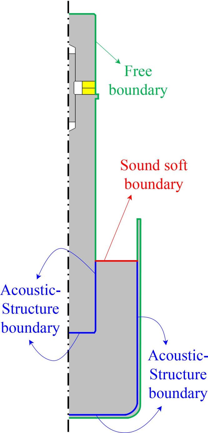
Mechanical boundary conditions for the solid and acoustic boundary conditions for the liquid. The blue lines couple the liquid acoustics to the solid vibrations. The yellow rectangles are the piezo-electric rings.
The exact value of the operating frequency used in experiments is not exactly known, but is set automatically by the generator. The strategy used in practice ensures that the impedance of the transducer motionnal branch is purely resistive [69]. This feature is implemented in our model as described in Ref. [42] and the operating frequency is computed as a model output [43].
The numerical modeling was performed in a 2D-axisymmetric geometry. The model yields the acoustic pressure field in the cylindrical coordinates , which can be viewed as the acoustic field in the vessel mid-plane. A first naive side-to-side comparison of our numerical results with luminol maps would consist in sketching a color-plot of the acoustic pressure in those zones where Blake threshold is exceeded. A more elaborate comparison would require the computation of the number of radicals OH produced by the bubbles. Since our bubble model does not account for sonolysis kinetics, this remains unfeasible directly. However, Hegedüs and co-workers proposed an interesting universal scaling-law relating the OH reaction rate to the expansion ratio [70], which may have been usable here since our bubble dynamics code provides this ratio in function of acoustic pressure. Nevertheless, in a more recent paper, the same authors stressed the need to actualize the reaction kinetics models and account for large pressure effects in order to get more realistic prediction of the sonolysis products [71]. Unfortunately, they did not recompute their scaling-law on the their new results. We chose therefore an in-between solution, consisting in color-plotting side-to-side with luminol maps the collapse temperature of the bubbles, the latter quantity being directly available as an output of our external bubble-dynamics code in function of acoustic pressure. The underlying assumption, a priori reasonable, is that the radicals production rate is an increasing function of the collapse temperature above the Blake threshold.
4. Results and discussion
4.1. Effect of the transducer immersion
Fig. 4 show the electrical power () and calorimetric power () for experiment set 1, measured (points with errorbars) and computed (solid/dashed lines) in function of the distance from transducer to vessel bottom , for the three vessels. Note that on the latter figures, the transducer immersion depth increases from right to left.
Fig. 4.

Experiments set 1: comparison between simulated and experimental electrical and calorimetric power in function of distance from transducer to bottom for the vessels A, B and C (liquid volume was 836 mL, 1818 mL, and 1767 mL for the vessels A, B and C, respectively; input current was 0.6A; and all the data points have error bars).
The calorimetric power follows the same evolution as the electrical power, both for computed and measured values, with a yield close to 70% for all experimental points. This means that despite the large variety of experimental conditions, the command strategy of the transducer ensures an almost constant yield, and this is reasonably well predicted by our model. However our numerical predictions always overestimate the electrical and calorimetric powers by a factor of about 2. This mismatch was already reported and discussed for the electrical power in an earlier paper [43]. Since the present result show the same tendency for the calorimetric power, this discards a potential origin of the problem in modelling dissipation in the transducer, and definitely confirms that our cavitating liquid model overestimates dissipation.
The calorimetric powers are displayed for the three vessels on Figs. 4 a,b,c, in function of the distance from vessel bottom to transducer . Note that the transducer immersion depth increases when reading these figures from right to left. As a general feature for the three vessels, the computed (solid lines) increases as decreases below a threshold value, i.e., when the immersion depth exceeds a certain threshold. For vessel A (Fig. 4a), both the experimental and computed values show a consistent trend, demonstrating a monotonic increase in both calorimetric and electrical powers as decreases from 80mm down to 30mm. This is no longer the case for vessels B and C (Fig. 4, Fig. 4), for which the experimental power exhibits some noticeable oscillations in function of immersion depth.
In a precedent work [43], the almost monotonic increase of calorimetric power for vessel A was attributed to the gradual growth of the cavitation zone on the lateral sides of the transducer as immersion increases, which is indeed typically observed in similar experimental setups [50]. However, examination of luminol maps for this experiment (Fig. 5, left half-parts of pictures) reveals phenomena more complex than the simple appearance of lateral structures (the reader interested in the original unsymmetrized luminol figures without the comparison with numerical results is referred to supplementary material, Fig. S1). The lateral structures remain indeed very thin and sticked to the transducer for ), whereas our model predicts an initially large lateral zone monotonically disappearing as immersion depth decreases (Fig. 5, right half-parts of pictures). The thin lateral zone completely disappears for , and suddenly reappears with a spatial extension more or less constant up to . For , it seems to merge with a secondary luminol spot forming an arc-shaped structure (see the full luminol figure Fig. S1 in supplementary material for an easier appreciation), which interestingly is qualitatively caught by our simulation. With further decreasing immersion depth (), this structure gradually vanishes both in luminol maps and in our numerical prediction. This analysis reflects that complex acoustic phenomena are at work in the vessel, beyond the presence or absence of lateral structures, and that correlating the luminol zones (Fig. 5)) to the power curves (Fig. 4a) remains difficult. Counter-intuitively, the appearance of a secondary luminol bright zone above the vessel bottom for some specific immersion depths () even corresponds to a minimum of the calorimetric power. It should be noted that our model also wrongly predicts the appearance of this secondary active zone above the vessel bottom almost for all immersion depths. As well, no convincing correlation between the latter and the computed calorimetric power curve can be established.
For vessels B and C, as the liquid volume is larger, the number of excitable acoustic modes increases, possibly leading to more complex field patterns in the vessel. This is particularly clear for vessel B (Fig. 6 and full luminol maps in supplementary material), whose large height allows the appearance of secondary bright zones not only near the vessel bottom, but also at other points on the symmetry axis (see for example ). The appearance/disappearance of these secondary zones and their variable intensity are predicted by our model, but do not closely match experimental glowing luminol regions. They are even erroneously predicted for immersion depths at which they do not appear experimentally (for example ).
Fig. 6.

Experiments set 1, vessel B: SCL emission (left part of images) and predicted collapse temperature field (right part of images) at different immersion depths. The input current was and the liquid height computed from Eq. (1).
Contrarily to vessel A, a naked-eye examination of the luminol maps for vessel B (see supplementary material Fig. S2) and the corresponding power curve (Fig. 4b) reveals the rather intuitive conclusion that the global number of photons emitted by luminol matches the dissipated power (especially the maximum for and the minimum for ). This remains approximately true for vessel C (Figs. 4c and S3 in supplementary material), especially the decreasing power in the ranges 30mm to 60mm and 90mm to 130mm. Why this is not the case for vessel A remains rather surprising.
In the range for vessel B (pictures 8 to 12 in Fig. 6), an elongated luminol structure appears under the transducer, associated with lateral bright zones approximately at the level of the transducer tip, evoking an elephant head with trunk and ears (see Fig. S2 in supplementary material). Interestingly, an increase of the dissipated power can be observed in this range (Fig. 4b). A similar observation, albeit less blatant, can be made for vessel C (Figs. 7 and S3 in supplementary material) in the range , which again corresponds to a local maximum in the dissipated power curve (Fig. 4c). It can be noted that this elongated structure was never captured by our model.
Fig. 7.

Experiments set 1, vessel C: SCL emission (left part of images) and predicted collapse temperature field (right part of images) at different immersion depths. The input current was and the liquid height computed from Eq. (1).
As a final remark on the effect of immersion depth, examination of the power curves leads to a useful conclusion, generally overlooked in sonochemistry experiments and industrial scale-up considerations: maintaining a constant input current, which corresponds to a particular position of the generator’s ”power level” button, does not guarantee a constant calorimetric power. As a result, because the volume of the liquid stays constant, two experimenters using the same graduation level but different immersion depths would perform sonochemical tests with significantly different dissipated powers, and probably different chemical yields. This is especially evident for vessels B and C (Fig. 4, Fig. 4c): even avoiding ”extreme” configurations where the transducer tip is either very close to the liquid free surface or near the vessel bottom, calorimetric power can still vary by a factor 2 for intermediate positions. This demonstrates the importance of the geometric effects investigated in the present paper.
4.2. Effect of the liquid height
Experiment set 2 investigates the effect of varying the liquid heigth. Previous studies [59], [72], [58], [73] have reported an increase of calorimetric power and cavitation production with the liquid height, for the same input electrical power in bath-type sonoreactors. Whereas our computed values clearly follow this trend (Figs. 8), this is not the case for the experimental calorimetric powers, except for vessel A. For vessel B and C, the calorimetric power curves exhibit a hump (in the range for vessel B, and for vessel C) superimposed with a global increase with liquid height. Our model fails in predicting these humps, and here again, our computed values are overestimated by the same order of magnitude as for experiment set 1.
Fig. 8.

Experiment set 2: comparison between simulated and experimental electrical and calorimetric power in function of liquid level for the vessels A, B and C (the distance between the transducer’s tip and the vessel’s bottom was 20 mm, 80 mm, and 30 mm for the vessels A, B and C, respectively; input current was 0.6A; and all the data points have error bars).
The luminol maps for vessel A (Fig. 9 and S4), reveals the progressive appearance of a lateral bright zone at a liquid height of , slightly increasing up to . While our model predicts reasonably well this feature, it fails in predicting its sudden disappearance at . Instead, numerical computations predicts an ever increasing lateral bright zone as the liquid level increases, whose experimental counterpart was not observed, despite a tiny bright zone sticked to the transducer lateral walls can again be observed in the range 100 mm to 125 mm. Similar conclusions can be drawn for vessels B and C (Fig. 10, Fig. 11): lateral bright zones appear and disappear in a rather non-intuitive way as liquid level increases, whereas our model predicts their smooth appearance and evolution. In some occasions our model can reproduce surprisingly well the presence and even the shape of lateral zones (Fig. 10 for and Fig. 11 for but yields wrong predictions of lateral zones as a general trend, noticeably their sudden extinction for vessel C at between two windows of existence (Fig. 11, see also Fig. S6 in supplementary material). The latter feature was found to correspond to a slight increase of the experimental frequency (about 10Hz) chosen by the generator for these two liquid heights. Despite our model is built to account for automatic frequency selection, it fails here in doing so, which might results in an incorrect prediction of lateral activity.
Fig. 9.

Experiments set 2, vessel A: SCL emission (left part of images) and predicted collapse temperature field (right part of images) at different liquid levels. The input current was and the distance between the transducer’s tip and the vessel’s bottom .
Fig. 10.

Experiments set 2, vessel B: SCL emission (left part of images) and predicted collapse temperature field (right part of images) at different liquid levels. The input current was and the distance between the transducer’s tip and the vessel’s bottom .
Fig. 11.

Experiments set 2, vessel C: SCL emission (left part of images) and predicted collapse temperature field (right part of images) at different liquid levels. The input current was and the distance between the transducer’s tip and the vessel’s bottom .
It is worth noting that, similar to experiment set 1, the hump appearing in the calorimetric power curve for vessel B once again corresponds to the appearance of elongated axial structures on the luminol maps, in the range for vessel B (Fig. 8, Fig. 10 and S5 in supplementary material). This is less obvious for vessel C, for which these elongated structures are anyway more difficult to assess owing to the proximity of the transducer tip to the vessel bottom.
4.3. Effect of the input current
Using the same methods, experiment set 3 examines the influence of the input current (ranging from 0.08 to 0.80A). The transducer was positioned at for vessels A, B, and C, respectively. Those heights were chosen semi-empirically by selecting the richest structures observable on the luminol maps of experiment set 1 (Fig. 5, Fig. 6, Fig. 7, or S1, S2 and S3 in supplementary material).
Experiments at constant geometry are interesting because in this case, the acoustic eigenmodes of the system constituted by the liquid and vessel walls are the same for all experiments. As the driving current is increased, cavitation sets and adds some non-linearity to the reactor acoustics, and observing the corresponding evolution of luminol maps may help to elucidate this complex phenomenon.
Fig. 12a displays the monotonic increase of the experimental electrical and calorimetric powers as the input current is increased. The numerical predictions again overestimates the energy dissipated by cavitation in the liquid by a factor of approximately two. Similar conclusions can be drawn for vessels B and C, as depicted by Fig. 12, Fig. 12c.
Fig. 12.

Experiments set 3: comparison between simulated and experimental electrical and calorimetric power in function of input current for the vessels A, B and C (liquid volume was 836 mL, 1818 mL, and 1767 mL for the vessels A, B and C, respectively; the distance between the transducer’s tip and the vessel’s bottom was 60 mm, 110 mm, and 80 mm for the vessels A, B and C, respectively; and all the data points have error bars).
For vessel A, luminol maps reveals the progressive build-up and growth of three cavitation zones upon increasing the input current (Fig. 13 and Fig. S7 in supplementary material). One is located below the transducer tip, a secondary zone corresponding to a local pressure antinode appears above the vessel bottom, plus a lateral zone similar to the ones observed in experimental sets 1 and 2. Except for the latter, all zones shapes are reasonably well predicted by our model up to , despite closer examination of the full luminol zones (Fig. S7, supplementary material) reveal experimental shapes flatter than our prediction. From this value and above, the tip zone turns into an elongated structure similar to the ones already mentioned for experiment sets 1 and 2, with a concomitant change in the shape of the bottom zone. As for experiment sets 1 and 2, our prediction of the luminescent zones becomes worse as soon as these elongated zones appear. Similar conclusions can be drawn for the other vessels (Fig. 14, Fig. 15), except that whereas our numerical prediction for vessel B yields acceptable results for low driving currents, the computed fields for vessel C noticeably differ from the experimental structures even at low driving current. An interesting feature can also be observed for vessel B (Figs. 14 and S8 in supplementary material): above some threshold current (), all lateral secondary structures disappear, and the luminol bright zone restricts to a jet-like structure almost constant in shape, despite the calorimetric power still increases with current, as shown by Fig. 12b.
Fig. 13.

Experiments set 3, vessel A: SCL emission (left part of images) and predicted collapse temperature field (right part of images) for different input currents. The distance between the transducer’s tip and the vessel’s bottom and the liquid volume was 836ml.
Fig. 14.

Experiments set 3, vessel B: SCL emission (left part of images) and predicted collapse temperature field (right part of images) for different input currents. The distance between the transducer’s tip and the vessel’s bottom and the liquid volume was 1818ml.
Fig. 15.

Experiments set 3, vessel C: SCL emission (left part of images) and predicted collapse temperature field (right part of images) for different input currents. The distance between the transducer’s tip and the vessel’s bottom and the liquid volume was 1767ml.
Finally, for all vessels, our model predicts a lateral zone of almost constant shape and location, smoothly growing as current increases. In contrast, the experimental luminol maps reveal a much more complex evolution for vessel A (Fig. 13), with a merging process with the bright structure under the tip. Furthermore, for almost all currents above 0.44A, an additional small bright spot appears near the transducer corners (see Fig. S7, supplementary material). For vessel B (Fig. 14), lateral structures are almost nonexistent, in contrast with our prediction, but curiously, for vessel C (Fig. 15), the observed lateral structures are in correct agreement with our prediction.
4.4. Discussion
The results of experiments set 3 reveal that upon increasing the driving current, the shape of luminol spots switches between two states at a given threshold. At small drivings, the variety bright zones observed for the different vessels are reminiscent of linear acoustics antinodal zones in standing waves, that would correspond to a combination of eigenmodes of the liquid volume coupled with vessel walls. Preliminary computations seem to confirm this hypothesis but deeper investigation is ongoing. Above the threshold, an universal jet-like elongated bright luminol structure always appears below the transducer, for the three vessels. This structure overlaps with those structures that were existing below the threshold, interacting either weakly with them (vessel A, Figs. 13 and S7), or more strongly, even killing them completely in some cases (vessel B, Figs. 14 and S8). No sign of this transition between the two states is visible on the calorimetric power curves.
This elongated structure was also found for some specific ranges of geometries in experimental sets 1 and 2, appearing and disappearing as either the immersion depth or liquid level were varied. Since an intermediate driving current () was used for the latter experiments, this is consistent with the observations of experiment set 3: the threshold is geometry-dependent so that when varying geometry at constant current, the latter may fall either below or above the threshold. There is also some evidence that the occurrence of the elongated structure is concomitant with a noticeable increase of calorimetric power.
These results suggest that two regimes may be found in sonoreactors, both making luminol glow and involving cavitation. In the first one, reminiscence of linear acoustics is visible with luminol bright zones materializing the antinodes of a standing wave pattern, built on a combination of close eigenmodes. In the second, this standing wave pattern would be dominated or even completely destroyed by non-linearity associated with the onset of a strong cavitation cloud under the transducer, that would dissipate a large energy.
The reason why the second state would result in an elongated luminol structure might be connected with the onset of acoustic streaming, which would transport the excited species in a downward-flowing jet. If this interpretation was correct, this would suggest that a glowing luminol zone does not always indicate regions of strong cavitation, but also downstream zones in the streaming flow, where cavitation may be absent, but still contain excited luminol products coming from upstream cavitation zones. The luminol figures recorded by Son and co-workers [74] suggest a similar conclusion, as they show bright jets extending down to the vessel bottom and splashing on the latter. The concomitance of strong acoustic streaming with a strong cavitation field under the transducer is supported by theory since the driving force for streaming is directly connected with the strong energy dissipated by cavitation [75].
An alternative mechanism responsible for the existence of two distinct states in the sonoreactors should be mentioned. As suggested by the numerical results of Vanhille & Campos-Pozuelo [76], the bubbly layer located under the transducer may be either acoustically transparent or opaque to waves, by a nonlinear dispersive effect. Opacity arises from the fact that the layer becomes resonant for some specific value of the bubble density, because the corresponding value of the bubbly liquid sound speed makes an integer number of half-wavelengths casting into the layer thickness. Such effects may not be ruled out, but cannot observed with our model, since the huge dissipation predicted by the latter overwhelms them. Additionally, the computation of Ref. [76] involve acoustic pressures well below the Blake threshold and whether such effects still exist in presence of inertial cavitation is yet unknown.
Finally, our model was found to fail in predicting this second regime. If streaming is indeed involved, predicting correctly the luminol maps would require the computation the streaming velocity field, which can be done easily using the model described in Ref. [75], but also to solve a convection–diffusion-reaction equation for luminol transfer. To do so, the chemical kinetics of luminol de-excitation would be required. Whether a such complex model is viable remains debatable but a semi-empirical approach is under investigation.
Beyond the precise prediction of luminol maps, our model fails anyway in predicting the maxima observed on the calorimetric power in set 1, concomitant with the appearance of elongated structures. However, it should be noted that for some geometric configurations, it yields remarkably realistic predictions in state 1, especially for the lateral structures near the transducer (see for example Fig. 6 for , Fig. 7 for , and Fig. 10 for ). Why this is not the case for all geometries is yet unclear.
Our model of cavitating liquid can of course be challenged, and several paths of amelioration were proposed in Ref. [43], which we remind quickly here. Louisnard chose to set the real part of the square wave number to its linear value (6) and argued that its precise value was not significant since contains the main energy dissipation mechanism and is large [39]. However, later studies showed that could be also computed in a nonlinear context [77], [78]. Sojahrood and co-corkers refined the results for nonlinear acoustical properties of bubbly liquids [79] and extended the theory to liquids seeded with coated bubbles [80]. Recently, they remonstrated that was also pressure dependent, and probed their theoretical results against experiments with coated bubbles of well-controlled size [81], which the first experimental verification of Louisnard’s approach. Interestingly for the present work, they showed that the drop of for increasing acoustic pressure could reduce attenuation by a twofold factor, which might explain both our overestimation of the dissipated power and the failure of our model in predicting some standing-wave like luminol map structures. Correcting our model to account for the correct calculation of can be easily done in a short term. Another source of discrepancy may lie in the non-accounting for bubble–bubble interactions in our model, beyond the one already inherently caught by Caflisch model. This issue was also addressed for by Sojahrood [82], [81] and others [83]. A clean implementation of such complexity in our model seems more difficult even if simplified approaches have been proposed [84], [85]. Finally, we feel that the crudest assumption in our model is bubble sphericity. The theoretical parametric space for spherical bubbles above Blake threshold is very narrow [68], [86], [87], [88] and observations reveal that sphericity is rather the exception than the rule [89], [90]. In particular most bubbles undergo jetting upon collapse and probably dissipate less energy than we compute, since it can be checked that the major part of viscous energy dissipation appearing in expression (7) originates from collapse.
Additionally, the influence of the vessel walls can also be suspected. Indeed, the flexural modes they undergo is very sensitive to their thickness, whose precision cannot be guaranteed to less than a few tenth of millimeter, and might not even be uniform. Preliminary computations show that a variation of can yield noticeable variations in the eigenmodes of the filled vessel. This constitutes an unexpected issue in sonoreactors modelling, that deserves further investigation.
5. Conclusion
In this study, we have investigated the effect of transducer immersion depth, liquid height, and input current on the sonochemical activity in three 20kHz sonoreactors of different shapes. Calorimetric power and luminol maps were recorded for a total of 183 experiments. Luminol maps were corrected for refraction effects. All configurations have been simulated with a non-linear model of cavitating liquid accounting for the vessel walls, the transducer and the strategy of command of the latter.
It was observed that the calorimetric power follows a similar trend as the electrical power, with a consistent yield of approximately 70% across different experimental conditions. This indicates that the command strategy of the transducer ensures a nearly constant yield, as predicted by our model. However, our numerical predictions overestimate both the electrical and calorimetric powers by a factor of about 2. This discrepancy, previously reported for the electrical power [43], suggests that our cavitating liquid model overestimates dissipation by cavitation bubbles.
The variation of liquid level at constant liquid volume and driving current (i.e. constant amplitude graduation on the generator) unambiguously show that the dissipated power can change by a factor 2 when changing the transducer immersion depth, with a non-monotonic relation between the two quantities. This stresses the importance of the geometric effects for the design and optimization of sonoreactors.
Luminol maps unveiled complex non-intuitive structures, including the appearance, disappearance, and merging of various luminol zones in function of geometry. A universal feature is the appearance of elongated axial structures in some parametric windows, accompanied by a noticeable increase of the calorimetric power. Experiments at fixed geometry and variable current unraveled that this state appears above a driving amplitude threshold, and may be due to a strong cavitation cloud below the transducer dissipating a lot of energy and promoting the onset of acoustic streaming, responsible for the observed elongated shape. Below the threshold, luminol maps exhibit shapes reminiscent of standing wave patterns. The latter can either survive and interact with the elongated structure when the threshold is exceeded, or completely disappear. These observations suggest that the acoustics of sonoreactors is a complex interplay between linear resonance modes of the liquid/vessel walls system and non-linearity produced by cavitation.
Our model was originally designed to account for such a complex interaction since it contains both linear acoustics in bubble-free regions and non-linear dissipative acoustics in bubble-populated zones. In spite of this feature and the thorough modelling of the vessel walls, transducer and command strategy, it was unable to fully catch the experimental results. However, some luminol structures, especially the lateral near-transducer bright zones, were remarkably well reproduced in some cases, but not for all experiments. Failures may be attributed to our cavitation model, but also to an inexact representation of the vessel wall flexion modes, owing to their sensitivity to the walls thickness.
These results highlight the need for further investigations to better understand and model the intricate acoustic phenomena involved in sonoreactors. The present findings have implications for sonochemistry experiments and industrial scale-up considerations, and underline the importance of geometric effects in cavitation systems.
CRediT authorship contribution statement
Igor Garcia-Vargas: Conceptualization, Methodology, Software, Investigation, Data curation, Writing - original draft. Olivier Louisnard: Conceptualization, Methodology, Software, Validation, Formal analysis, Investigation, Resources, Data curation, Writing - review & editing, Supervision, Project administration, Funding acquisition. Laurie Barthe: Conceptualization, Methodology, Resources, Supervision, Project administration, Funding acquisition.
Declaration of Competing Interest
Olivier Louisnard reports financial support was provided by SinapTec to RAPSODEE center at IMT Mines-Albi. Laurie Barthe reports financial support was provided by SinapTec to the Laboratoire de Génie Chimique. Igor Garcia-Vargas reports a relationship with SinapTec that includes: employment and funding grants. The above-mentioned authors declare that they had full access to all of the data in this study and take complete responsibility for the integrity of the data and the accuracy of the data analysis.
Acknowledgements
The authors gratefully acknowledge SinapTec for financially supporting the research through an industrial PhD grant (N 2019/1344) awarded to Igor Garcia-Vargas by the French Association Nationale de la Recherche et de la Technologie (ANRT). Special thanks are extended to Jean-Pierre Escafit and Bruno Boyer from LGC for their valuable technical support with the experimental setup. Additionally, the authors would like to acknowledge the French Centre National de la Recherche Scientifique (CNRS) for supporting the cavitation research group (GDR CAVITATION), which facilitated fruitful discussions with colleagues in the field.
Footnotes
Supplementary data associated with this article can be found, in the online version, athttps://doi.org/10.1016/j.ultsonch.2023.106542.
Appendix A. Correction of optical aberrations
A.1. Main concept
Before experiment, the vessel is filled with water, and the camera is focused by the naked-eye in the mid-plane of the vessel by ensuring that the the lateral part of the immerged transducer appears sharp. This means that all rays emerging from a point M in water in the mid-plane must focus on the sensor after having being refracted by the water/glass and glass/air interfaces (see Fig. A.16). As these rays are deflected, they seem to emerge from a point (the virtual object) which is located further away from the optical axis, and closer to the cylinder vertex V than it actually is. The plane containing is the object plane. Any object located in air in this plane would appear sharp on the image. Note that Fig. A.16 is an over-simplification since rays are not contained in the figure plane and also have a vertical component.
Fig. A.16.

Sketch of the optical system view from above. The optical axis, and all optical data are sketched in red. The camera lens is assumed equivalent to a simple thin lens with optical center and focal length . The vessel midplane is at distance from sensor. A point M in the vessel mid-plane is imaged at point P on sensor, and seems to originate from point . The latter is located in the object plane, at distance from the sensor, where is the object distance and the image distance. Among all the rays travelling from M to P (pink lines), the chief ray (blue line) crosses the optical center and is undeviated.
The above reasoning is however approximate. In fact, all rays emerging from M do not back-focus on a single point . This is due to the curvature of the vessel, which makes those rays hitting the cylinder wall far from the vertex converge to a different point than those hitting the cylinder wall close to the optical axis. This is already true for objects located on the optical axis, in which case this effect is known as spherical aberration, and is further complex for off-axis objects [61]. Such optical aberrations render the reconstruction by ray-tracing involved, if ever feasible.
The approximate treatment proposed relies on the small aperture () used in the present experiments. One might therefore assume that all the rays emerging from point M entering the camera through the small diaphragm aperture have very close directions. Thus, it is enough to consider only that incoming ray entering the diaphragm through the lens origin (so-called “ chief ray”, sketched in blue on Fig. A.16), ending at P on the sensor. It is then assumed that all the other rays emerging from M, able to enter the diaphragm aperture (pink lines on Fig. A.16), are sufficiently close to the chief ray so that they would all hit the sensor at the same location, and form there a sharp image P of the object located at M.
The practical method consists therefore in a backward computation of rays: a single ray is launched from each pixel on the sensor through the lens origin up to the vessel external wall, and its further refracted path through glass and water is computed using the Snell-Descartes law twice. We then compute the intersection point of the ray obtained in water with the vessel midplane. Note that the image obtained on sensor is reversed owing to central symmetry around optical center .
A.2. Calibration and alignment
The origin of space O is taken at the geometric center of the vessel internal bottom wall. The x-axis is the optical axis oriented toward the sensor, z is the vertical direction and y is chosen so that the trihedron is right-handed. No specific alignment between the sensor and the vessel midplane is assumed, except that they are parallel. The intersection point C of the optical axis with the vessel midplane must therefore be determined beforehand in a calibration procedure. The latter is made on an ambient-light picture of the filled vessel, and allows to select the vessel bottom and apparent external boundaries. From there a magnification G is deduced.
Furthermore, to perform correctly the computation of rays, the position of the object plane () and image plane must be known precisely. Since the camera does not provide any reliable information on the latter, these quantities are deduced from magnification. Starting from thin lens equations [61]:
and using , we get the following expressions:
| (A.1) |
| (A.2) |
| (A.3) |
The precise lens focal was measured precisely by an independent calibration experiment and was found to be instead of the 50mm commercial value.
A.3. Interpolation of pixels
From the rays computation, we get the position of the object coordinates in the vessel midplane which is imaged at point on the sensor. The color on the corrected image therefore fulfills:
Owing to refraction, a straight line in the midplane is imaged as a curve on sensor, and vice versa, so that back-launching rays from a rectangular grid on sensor yields scattered object points in the midplane. We therefore define a rectangular grid covering the latter and we seek the value of by interpolation between the scattered objects .
It should be noted that among the points in the liquid mid-plane, some are not imaged on the sensor because they are to close to the lateral wall of the vessel, and the ray they emit does not manage to leave the vessel towards the sensor. In other words there exists values of in the liquid midplane that cannot be mapped to a point on the sensor. This yields an “invisible zone” in water where luminol may glow but cannot be imaged. Such zones are represented in white on the reconstructed image.
A.4. Drawbacks of the method
Apart from the approximation of considering a single ray, the following drawbacks can be enumerated:
-
1.
Luminol emitters are scattered in the whole liquid, not only in the mid-plane. Since the depth of field is extended, emitters ahead of or behind the midplane also emit light, which is imaged by the sensor as well, even if, being out of focus, they do not form a sharp image. Considering that each sensor pixel only images luminol emitters located in the midplane is clearly an abusive hypothesis. Note that this is a general problem for luminol imaging which is not specific to the present method. This yields unrealistic imaging for out-of-axis structures such as those appearing near the transducer side, which are toroidal and appear as a large rectangle in the whole liquid (Figs. 11 or S6 in supplementary material for ).
-
2.
Spurious reflections of luminol emission on the vessel cannot be avoided. This can be observed for example on the last images of Fig. 10 (or S5 in supplementary material), where the apparent luminol structure near the vessel bottom results in fact from perspective and complex reflexions on the bottom.
-
3.
Our method assumes for now that the vessel walls are concentric perfect cylinders. It does not account for the round fillet joining the bottom of the vessel to its lateral walls. This may produce substantial refraction effects and influence the apparent location and shapes of the glowing zones located close to the bottom. Accounting for this feature is straightforward from the modelling point of view but requires more CPU time to compute the rays. This will be corrected in the next version.
Appendix B. Supplementary data
The following are the Supplementary data to this article:
References
- 1.Matouq M.A.-D., Al-Anber Z.A. Ultrason. Sonochem. 2007;14(3):393–397. doi: 10.1016/j.ultsonch.2006.09.003. [DOI] [PubMed] [Google Scholar]
- 2.Agarkoti C., Thanekar P.D., Gogate P.R. J. Environ. Manage. 2021;300 doi: 10.1016/j.jenvman.2021.113786. [DOI] [PubMed] [Google Scholar]
- 3.Vinatoru M. Ultrason. Sonochem. 2001;8(3):303–313. doi: 10.1016/s1350-4177(01)00071-2. [DOI] [PubMed] [Google Scholar]
- 4.Nguele R., Okawa H. Ultrason. Sonochem. 2021;80 doi: 10.1016/j.ultsonch.2021.105811. [DOI] [PMC free article] [PubMed] [Google Scholar]
- 5.Chen Y., Zheng H., Truong V.N.T., Xie G., Liu Q. Ultrason. Sonochem. 2020;63 doi: 10.1016/j.ultsonch.2019.104924. [DOI] [PubMed] [Google Scholar]
- 6.Guo C., Liu J., Li X., Yang S. Ultrason. Sonochem. 2021;79 doi: 10.1016/j.ultsonch.2021.105782. [DOI] [PMC free article] [PubMed] [Google Scholar]
- 7.Girard M., Bertrand F., Tavares J.R., Heuzey M.-C. Ultrason. Sonochem. 2021;78 doi: 10.1016/j.ultsonch.2021.105747. [DOI] [PMC free article] [PubMed] [Google Scholar]
- 8.Luque de Castro M.D., Priego-Capote F. Ultrason. Sonochem. 2007;14(6):717–724. doi: 10.1016/j.ultsonch.2006.12.004. [DOI] [PubMed] [Google Scholar]
- 9.Li H., Li H., Guo Z., Liu Y. Ultrason. Sonochem. 2006;13(4):359–363. doi: 10.1016/j.ultsonch.2006.01.002. [DOI] [PubMed] [Google Scholar]
- 10.L. d. l. S. Castillo-Peinado, M.D.L. de Castro, Journal of Pharmacy and Pharmacology 68 (10) (2016) 1249–1267. [DOI] [PubMed]
- 11.Mohsin M., Meribout M. Ultrason. Sonochem. 2015;22:573–579. doi: 10.1016/j.ultsonch.2014.05.014. [DOI] [PubMed] [Google Scholar]
- 12.Modarres-Gheisari S.M.M., Gavagsaz-Ghoachani R., Malaki M., Safarpour P., Zandi M. Ultrason. Sonochem. 2019;52:88–105. doi: 10.1016/j.ultsonch.2018.11.005. [DOI] [PubMed] [Google Scholar]
- 13.Gaete-Garretón L., Briceño-Gutiérrez D., Vargas-Hernández Y., Zanelli C.I. J. Acoust. Soc. Am. 2018;144(1):222–227. doi: 10.1121/1.5045558. [DOI] [PubMed] [Google Scholar]
- 14.Mc Carogher K., Dong Z., Stephens D.S., Leblebici M.E., Mettin R., Kuhn S. Ultrason. Sonochem. 2021;75 doi: 10.1016/j.ultsonch.2021.105611. [DOI] [PMC free article] [PubMed] [Google Scholar]
- 15.Naidu H., Kahraman O., Feng H. Ultrason. Sonochem. 2022;86 doi: 10.1016/j.ultsonch.2022.105984. [DOI] [PMC free article] [PubMed] [Google Scholar]
- 16.Price G.J., West P.J., Smith P.F. Ultrason. Sonochem. 1994;1(1):S51–S57. [Google Scholar]
- 17.T.G. McKenzie, F. Karimi, M. Ashokkumar, G.G. Qiao, Chemistry – A European Journal 25 (21) (2019) 5372–5388. [DOI] [PubMed]
- 18.Islam M.H., Burheim O.S., Pollet B.G. Ultrason. Sonochem. 2019;51:533–555. doi: 10.1016/j.ultsonch.2018.08.024. [DOI] [PubMed] [Google Scholar]
- 19.Zore U.K., Yedire S.G., Pandi N., Manickam S., Sonawane S.H. Ultrason. Sonochem. 2021;73 doi: 10.1016/j.ultsonch.2021.105536. [DOI] [PMC free article] [PubMed] [Google Scholar]
- 20.Gai W.-Z., Tian S., Liu M.-H., Zhang X., Deng Z.-Y. Ultrason. Sonochem. 2022;90 doi: 10.1016/j.ultsonch.2022.106189. [DOI] [PMC free article] [PubMed] [Google Scholar]
- 21.Mason T., Lorimer J. Chem. Eng. Process. 2003;9:885–900. [Google Scholar]
- 22.Iida Y., Yasui K., Tuziuti T., Sivakumar M. Microchem. J. 2005;80(2):159–164. [Google Scholar]
- 23.Wood R.J., Lee J., Bussemaker M.J. Ultrason. Sonochem. 2017;38:351–370. doi: 10.1016/j.ultsonch.2017.03.030. [DOI] [PubMed] [Google Scholar]
- 24.Pokhrel N., Vabbina P.K., Pala N. Ultrason. Sonochem. 2016;29:104–128. doi: 10.1016/j.ultsonch.2015.07.023. [DOI] [PubMed] [Google Scholar]
- 25.Leighton T.J. Academic Press; London: 1994. The acoustic bubble. [Google Scholar]
- 26.Mason T. Ultrasonics. 1992;30(3):192–196. [Google Scholar]
- 27.Berlan J., Mason T.J. Ultrasonics. 1992;30(4):203–212. [Google Scholar]
- 28.Mason T.J. Ultrason. Sonochem. 2000;7(4):145–149. doi: 10.1016/s1350-4177(99)00041-3. [DOI] [PubMed] [Google Scholar]
- 29.Gogate P.R., Sutkar V.S., Pandit A.B. Chem. Eng. J. 2011;166(3):1066–1082. [Google Scholar]
- 30.Rashwan S.S., Mohany A., Dincer I. Int. J. Hydrogen Energy. 2021;46(29):15219–15240. doi: 10.1016/j.ijhydene.2021.07.101. [DOI] [PMC free article] [PubMed] [Google Scholar]
- 31.Tiong T.J., Chandesa T., Yap Y.H. Ultrason. Sonochem. 2017;36:78–87. doi: 10.1016/j.ultsonch.2016.11.003. [DOI] [PubMed] [Google Scholar]
- 32.Tiong T.J., Liew D.K.L., Gondipon R.C., Wong R.W., Loo Y.L., Lok M.S.T., Manickam S. Ultrason. Sonochem. 2017;35:569–576. doi: 10.1016/j.ultsonch.2016.04.029. [DOI] [PubMed] [Google Scholar]
- 33.Chu J.K., Tiong T.J., Chong S., Asli U.A., Yap Y.H. Ultrason. Sonochem. 2021;80 doi: 10.1016/j.ultsonch.2021.105818. [DOI] [PMC free article] [PubMed] [Google Scholar]
- 34.Chu J.K., Tiong T.J., Chong S., Asli U.A. Chem. Eng. Sci. 2022;247 [Google Scholar]
- 35.Caflisch R.E., Miksis M.J., Papanicolaou G.C., Ting L. J. Fluid Mech. 1985;153:259–273. [Google Scholar]
- 36.Commander K.W., Prosperetti A. J. Acoust. Soc. Am. 1989;85(2):732–746. [Google Scholar]
- 37.Campos-Pozuelo C., Granger C., Vanhille C., Moussatov A., Dubus B. Ultrason. Sonochem. 2005;12(1):79–84. doi: 10.1016/j.ultsonch.2004.06.009. [DOI] [PubMed] [Google Scholar]
- 38.O. Louisnard, in: Physics Procedia, Vol. 3, 2010, pp. 735–742, international Congress on Ultrasonics, Santiago de Chile, January 2009.
- 39.Louisnard O. Ultrason. Sonochem. 2012;19:56–65. doi: 10.1016/j.ultsonch.2011.06.007. [DOI] [PubMed] [Google Scholar]
- 40.Louisnard O. Ultrason. Sonochem. 2012;19:66–76. doi: 10.1016/j.ultsonch.2011.06.008. [DOI] [PubMed] [Google Scholar]
- 41.Louisnard O., González-García J.J., Tudela I., Klima J., Saez V., Vargas-Hernandez Y. Ultrason. Sonochem. 2009;16:250–259. doi: 10.1016/j.ultsonch.2008.07.008. [DOI] [PubMed] [Google Scholar]
- 42.Louisnard O., Garcia-Vargas I. In: Energy Aspects of Acoustic Cavitation and Sonochemistry. Hamdaoui O., Kerboua K., editors. Elsevier; 2022. pp. 219–249. [Google Scholar]
- 43.Garcia-Vargas I., Barthe L., Tierce P., Louisnard O. Ultrason. Sonochem. 2022;91 doi: 10.1016/j.ultsonch.2022.106226. [DOI] [PMC free article] [PubMed] [Google Scholar]
- 44.Lind J., Merenyi G., Eriksen T.E. J. Am. Chem. Soc. 1983;105(26):7655–7661. [Google Scholar]
- 45.Henglein A., Ulrich R., Lilie J. J. Am. Chem. Soc. 1989;111(6):1974–1979. [Google Scholar]
- 46.Renaudin V., Gondrexon N., Boldo P., Pétrier C., Bernis A., Gonthier Y. Ultrason. Sonochem. 1994;1(2):S81–S85. doi: 10.1016/s1350-4177(98)00041-8. [DOI] [PubMed] [Google Scholar]
- 47.Hatanaka S.-I., Mitome H., Yasui K., Hayashi S. J. Am. Chem. Soc. 2002;124(35):10250–10251. doi: 10.1021/ja0258475. [DOI] [PubMed] [Google Scholar]
- 48.Ashokkumar M. Ultrason. Sonochem. 2011;18(4):864–872. doi: 10.1016/j.ultsonch.2010.11.016. [DOI] [PubMed] [Google Scholar]
- 49.Fernandez Rivas D., Ashokkumar M., Leong T., Yasui K., Tuziuti T., Kentish S., Lohse D., Gardeniers H.J.G.E. Ultrason. Sonochem. 2012;19(6):1252–1259. doi: 10.1016/j.ultsonch.2012.04.008. [DOI] [PubMed] [Google Scholar]
- 50.Son Y., No Y., Kim J. Ultrason. Sonochem. 2020;65 doi: 10.1016/j.ultsonch.2020.105065. [DOI] [PubMed] [Google Scholar]
- 51.Lee D., Na I., Son Y. Chemosphere. 2022;286 doi: 10.1016/j.chemosphere.2021.131780. [DOI] [PubMed] [Google Scholar]
- 52.Tuziuti T., Yasui K., Sivakumar M., Iida Y., Miyoshi N. J. Phys. Chem. A. 2005;109(21):4869–4872. doi: 10.1021/jp0503516. [DOI] [PubMed] [Google Scholar]
- 53.Tuziuti T., Yasui K., Kozuka T., Towata A., Iida Y. J. Phys. Chem. A. 2007;111(48):12093–12098. doi: 10.1021/jp077319r. [DOI] [PubMed] [Google Scholar]
- 54.Choi J., Son Y. Ultrason. Sonochem. 2022;82 doi: 10.1016/j.ultsonch.2021.105888. [DOI] [PMC free article] [PubMed] [Google Scholar]
- 55.Barchouchi A. Université Grenoble Alpes; These de doctorat: Sep. 2020. Réactivité sonochimique à l’interface solide-liquide. [Google Scholar]
- 56.Wells P.N.T., Bullen M.A., Follett D.H., Freundlich H.F., James J.A. Ultrasonics. 1963;1(2):106–110. [Google Scholar]
- 57.Mason T.J., Lorimer J.P., Bates D.M. Ultrasonics. 1992;30(1):40–42. [Google Scholar]
- 58.Asakura Y., Nishida T., Matsuoka T., Koda S. Ultrason. Sonochem. 2008;15(3):244–250. doi: 10.1016/j.ultsonch.2007.03.012. [DOI] [PubMed] [Google Scholar]
- 59.Son Y., Lim M., Ashokkumar M., Khim J. J. Phys. Chem. C. 2011;115(10):4096–4103. [Google Scholar]
- 60.McMurray H.N., Wilson B.P. J. Phys. Chem. A. 1999;103(20):3955–3962. [Google Scholar]
- 61.Hecht E. Pearson Education India; 2012. Optics. [Google Scholar]
- 62.I. Garcia-Vargas, L. Barthe, O. Louisnard, Light emission of luminol excited by acoustic cavitation, v1, URL:https://doi.org/10.57745/XI03JD Recherche Data Gouv (2023).
- 63.Borland D., Taylor R.M., II IEEE Comput. Graphics Appl. 2007;27(2):14–17. doi: 10.1109/mcg.2007.323435. [DOI] [PubMed] [Google Scholar]
- 64.S. Zeller, D. Rogers, Eos, Transactions American Geophysical Union 101.
- 65.M. Niccoli, Perceptually improved colormaps. MATLAB Central File Exchange., URL:https://www.mathworks.com/matlabcentral/fileexchange/28982-perceptually-improved-colormaps, [Online; Retrieved May 11, 2023] (2023).
- 66.Akhatov I., Gumerov N., Ohl C.D., Parlitz U., Lauterborn W. Phys. Rev. Lett. 1997;78(2):227–230. [Google Scholar]
- 67.Hilgenfeldt S., Brenner M.P., Grossman S., Lohse D. J. Fluid Mech. 1998;365:171–204. [Google Scholar]
- 68.Louisnard O., Gomez F. Phys. Rev. E. 2003;67(3) doi: 10.1103/PhysRevE.67.036610. [DOI] [PubMed] [Google Scholar]
- 69.K.F. Graff, in: J.A. Gallego-Juárez, K.F. Graff (Eds.), Applications of High-Intensity Ultrasound, 1st Edition, Woodhead Publishing series in electronic and optical materials, 2014, Ch. 6, pp. 127–158.
- 70.Kalmár C., Klapcsik K., Hegedüs F. Ultrason. Sonochem. 2020;64 doi: 10.1016/j.ultsonch.2020.104989. [DOI] [PubMed] [Google Scholar]
- 71.Kalmár C., Turányi T., Zsély I.G., Papp M., Hegedüs F. Ultrason. Sonochem. 2022;83 doi: 10.1016/j.ultsonch.2022.105925. [DOI] [PMC free article] [PubMed] [Google Scholar]
- 72.Son Y. Chem. Eng. J. 2017;328:654–664. [Google Scholar]
- 73.Asakura Y., Fukutomi S., Yasuda K., Koda S. J. Chem. Eng. Jpn. 2010;43(12):1008–1013. [Google Scholar]
- 74.Son Y., No Y., Kim J. Ultrasonics sonochemistry. 2020;65 doi: 10.1016/j.ultsonch.2020.105065. [DOI] [PubMed] [Google Scholar]
- 75.Louisnard O. Ultrasonics sonochemistry. 2017;35:518–524. doi: 10.1016/j.ultsonch.2016.09.013. [DOI] [PubMed] [Google Scholar]
- 76.Vanhille C., Campos-Pozuelo C. Ultrasonic Sonochemistry. 2009;16:669–685. doi: 10.1016/j.ultsonch.2008.11.013. [DOI] [PubMed] [Google Scholar]
- 77.A.J. Sojahrood, H. Haghi, R. Karshafian, M.C. Kolios, in: 2015 IEEE International Ultrasonics Symposium (IUS), IEEE, 2015, pp. 1–4.
- 78.Trujillo F.J. Ultrasonics sonochemistry. 2020;65 doi: 10.1016/j.ultsonch.2020.105056. [DOI] [PubMed] [Google Scholar]
- 79.Sojahrood A.J., Haghi H., Karshafian R., Kolios M.C. Ultrason. Sonochem. 2020;66 doi: 10.1016/j.ultsonch.2020.105089. [DOI] [PubMed] [Google Scholar]
- 80.Sojahrood A.J., Haghi H., Li Q., Porter T.M., Karshafian R., Kolios M.C. Ultrason. Sonochem. 2020;66 doi: 10.1016/j.ultsonch.2020.105070. [DOI] [PubMed] [Google Scholar]
- 81.Sojahrood A., Li Q., Haghi H., Karshafian R., Porter T., Kolios M. Ultrason. Sonochem. 2023;95 doi: 10.1016/j.ultsonch.2023.106319. [DOI] [PubMed] [Google Scholar]
- 82.A.J. Sojahrood, Q. Li, H. Haghi, R. Karshafian, T.M. Porter, M.C. Kolios, in: 2017 IEEE International Ultrasonics Symposium (IUS), 2017, pp. 1–4.
- 83.Doc J.B., Conoir J.M., Marchiano R., Fuster D. The Journal of the Acoustical Society of America. 2016;139(4):1703–1712. doi: 10.1121/1.4945452. [DOI] [PubMed] [Google Scholar]
- 84.Yasui K., Iida Y., Tuziuti T., Kozuka T., Towata A. Phys. Rev. E. 2008;77(1) doi: 10.1103/PhysRevE.77.016609. [DOI] [PubMed] [Google Scholar]
- 85.Yasui K., Lee J., Tuziuti T., Towata A., Kozuka T., Iida Y. J. Acoust. Soc. Am. 2009;126(3):973–982. doi: 10.1121/1.3179677. [DOI] [PubMed] [Google Scholar]
- 86.Mettin R. In: Oscillations, Waves and Interactions. Kurz T., Parlitz U., Kaatze U., editors. Universitätsverlag Göttingen; 2007. pp. 171–198. [Google Scholar]
- 87.Koch P., Kurz T., Parlitz U., Lauterborn W. J. Acoust. Soc. Am. 2011;130(5):3370–3378. doi: 10.1121/1.3626159. [DOI] [PubMed] [Google Scholar]
- 88.Klapcsik K., Hegedűs F. Ultrasonics sonochemistry. 2019;54:256–273. doi: 10.1016/j.ultsonch.2019.01.031. [DOI] [PubMed] [Google Scholar]
- 89.Cairós C., Mettin R. Physical review letters. 2017;118(6) doi: 10.1103/PhysRevLett.118.064301. [DOI] [PubMed] [Google Scholar]
- 90.Mettin R., Cairós C. Springer Singapore; Singapore: 2015. Bubble Dynamics and Observations; pp. 1–29. [Google Scholar]
Associated Data
This section collects any data citations, data availability statements, or supplementary materials included in this article.