

Abstract

Raman hyperspectral microscopy is a valuable tool in biological and biomedical imaging. Because Raman scattering is often weak in comparison to other phenomena, prevalent spectral fluctuations and contaminations have brought advancements in analytical and chemometric methods for Raman spectra. These chemometric advances have been key contributors to the applicability of Raman imaging to biological systems. As studies increase in scale, spectral contamination from extrinsic background, intensity from sources such as the optical components that are extrinsic to the sample of interest, has become an emerging issue. Although existing baseline correction schemes often reduce intrinsic background such as autofluorescence originating from the sample of interest, extrinsic background is not explicitly considered, and these methods often fail to reduce its effects. Here, we show that extrinsic background can significantly affect a classification model using Raman images, yielding misleadingly high accuracies in the distinction of benign and malignant samples of follicular thyroid cell lines. To mitigate its effects, we develop extrinsic background correction (EBC) and demonstrate its use in combination with existing methods on Raman hyperspectral images. EBC isolates regions containing the smallest amounts of sample materials that retain extrinsic contributions that are specific to the device or environment. We perform classification both with and without the use of EBC, and we find that EBC retains biological characteristics in the spectra while significantly reducing extrinsic background. As the methodology used in EBC is not specific to Raman spectra, correction of extrinsic effects in other types of hyperspectral and grayscale images is also possible.
Raman spectroscopy and hyperspectral microscopy continue to be valuable tools in many areas, including medicine,1,2 forensics,3,4 and materials.5 Raman microscopy, due to its capability as a high-resolution, label-free, and non-invasive imaging method, has been particularly useful in biological and biomedical applications.6−9 More recent advances have allowed Raman microscopy to be of use in subcellular imaging, in vitro imaging,10,11 and ex vivo tissue imaging12−14 and have much potential in imaging living systems.15 Because differences among Raman spectra of biological systems are often subtle, the utility of Raman images in biological applications has been aided by chemometrics.16−18 Many applications use classification models such as k-nearest neighbors (k-NN) and discriminant analysis,19 support vector machines,20 neural networks,17 and clustering.21 Other approaches use regression models to predict quantities such as pH22 or decrease measurement times through selective sampling.23
Many combinations of chemometrics and Raman measurements have been successful despite the prevalence of baseline, or background, contamination, interpreted here to be any intensity in a spectrum that does not arise from Raman scattering in the sample of interest. Some sources of background contributions are intrinsic to the sample, such as autofluorescence in cellular measurements, while other sources are extrinsic to the sample, such as fluorescence and scattering from optical components, sample media, and substrates. Many methods have been developed to mitigate background contamination, including those using polynomial regression,24,25 morphological operations,26,27 Bayesian learning,28 and mixture models.29 Other approaches seek optimal baseline estimates over multiple methods using genetic algorithms30 or quality measures.31 As studies increase in scale to include larger data sets, more measurements, and multiple devices, measurement-to-measurement differences, especially across devices, among Raman spectra are an emerging issue.32 A recent large-scale study33 emphasizes inconsistencies across different Raman devices, such as differences in positions, shapes, and/or intensities of characteristic Raman bands, leading to irreproducible artifacts. Standardization of Raman spectra across different measurements has included precise instrument calibration,34 modeling based on regression of Raman bands,35 and resolution matching with standard spectral libraries.36 Although these and more recent methods based in model transfer37,38 have shown potential in standardizing Raman spectra, contributions from extrinsic sources, e.g., optics, substrates, or sample media, that can lead to inconsistencies among devices and/or samples are not directly considered.
In this study, we demonstrate that extrinsic contributions can be estimated and corrected in many Raman hyperspectral images of biological samples as they often contain regions in which there is little sample, but extrinsic contributions are retained, such as the low-intensity areas between cells in in vitro biological samples. Similar to methods that separate background from foreground in traditional image and video processing,39 background pixels can be segmented, and their average spectrum was used to reduce extrinsic contamination in spectra having inconsistent extrinsic contributions. In the following, we develop extrinsic background correction (EBC) to estimate extrinsic background spectra in Raman images using the segmentation of background pixels.
We apply EBC to a set of Raman images containing in vitro human thyroid follicular epithelial cell cultures, including the malignant RO 82 W-1 cell line and the benign Nthy-Ori 3-1 cell line. Using a set of 50 Raman images containing nearly 250,000 individual Raman spectra, we demonstrate the adverse effects of extrinsic contributions in the recognition of cancerous and non-cancerous spectra on a classification model, k-NN, in the principal component (PC) space. It is found that spectral differences in optical components are learned by the k-NN model, leading to false discovery when spectra from different devices are used for cancer/non-cancer classification. In contrast, false distinction of cancerous and non-cancerous cell spectra in the classification model is reduced when EBC is used, even when cancerous and non-cancerous spectra originate from different devices. Considering the possibility of false discovery, reliable recognition of the device from which a spectrum originated by a classification model is an undesirable artifact. We therefore use device recognition as a measure of the efficacy of EBC using several existing baseline methods24−26 as comparative examples. The versatility of EBC is demonstrated through its use in concert with these existing baseline methods, and we find that device recognition is significantly reduced when EBC is used, regardless of the baseline method used or the cell line from which the spectra originate.
Computational and Experimental Methods
Extrinsic Background Correction
The key step in EBC is segmentation of the least intense group of pixels in the Raman image using a set of intensities I = {I1, ···, Ij, ···, IN} as an unsupervised clustering input, where each of the N intensities Ij represents a pixel j in the segmentation. Because photon counting is a Poisson process, the intensities I are expected to be drawn from Poisson distributions, and we seek the least intense Poisson distribution within the intensity set under the assumption that the extrinsic background spectrum is uniform across the sample. This has the benefit that other types of photon-counting data, such as hyperspectral fluorescence,40 nanoparticle scattering,41 grayscale images, or time trajectory data, are also suitable inputs to EBC. To generate the intensities to be segmented, from the discrete set of M measured wavenumbers, w = {w1, ···, wi, ···, wM}, we set to designate a subset of wavenumbers to be utilized for segmentation of the sample and non-sample regions. We note that the choice of segmentation subset wSS is dependent on the type of sample and adjustable to suit the sample of interest. Because Raman images of biological samples are used in this work, we select a subset of wavenumbers containing information about CH stretching vibrations of the CH2 and CH3 groups that are present in many biological molecules, wSS = {wi | 2840 cm–1 ≤ wi ≤ 2980 cm–1}, which is often the highest intensity region in the spectra. Using the spectrum sj(w) located at the individual pixel j, we define the intensity Ij to be the sum intensities in wSS, Ij = ∑wi ∈ wSSsj(wi). Repeating over all N pixels in the image, we obtain the set of intensities I for use in pixel segmentation.
In principle, the least intense Poisson distribution
in the set I can be obtained by initializing with
a single cluster and increasing the number of clusters K integer-wise until all clusters are approximately Poisson-distributed.
In Raman images of biological samples, however, some biochemical contributions
such as lipid droplets may be very bright and sparse in both the spatial
and intensity domains, causing some clusters to remain broader than
expected from Poisson intensities even if K is very
large. We therefore focus on the least intense cluster and increase K until this cluster has the properties of a Poisson distribution;
that is, its variance σ2 and mean μ are approximately
equivalent. Using the number of pixels NB belonging to this cluster as a sample size, the equivalence of μ
and σ2 is verified through a statistical test. A
sampling distribution for σ2 is computed using random
sampling of intensities from a Poisson distribution with mean μ
and sample size NB. To ensure sufficient
sampling, 10,000 sets containing NB intensities
are sampled, and their variances are estimated. The resulting set
of variances represents the distribution of variances that may be
observed from a Poisson sample with mean μ and NB samples. The equivalence of σ2 and
μ is assumed when σ2 falls within the central
95% confidence interval of the 10,000 randomly sampled variances.
The observed spectral intensities of the set of NB pixels belonging to the least intense cluster, denoted B, are used to estimate a background intensity at all wavenumbers,  , which is subsequently subtracted from
the observed spectral intensities at each pixel j, sj(w), to produce
a background-corrected intensity at each wavenumber, Ŝj(w) = sj(w) – b̂(w), thus completing EBC for the image. See Figure 1 for implementation of EBC on an experimental
Raman image.
, which is subsequently subtracted from
the observed spectral intensities at each pixel j, sj(w), to produce
a background-corrected intensity at each wavenumber, Ŝj(w) = sj(w) – b̂(w), thus completing EBC for the image. See Figure 1 for implementation of EBC on an experimental
Raman image.
Figure 1.

EBC. The sum intensity (A) mapping and (B) distribution for 2840–2980 cm–1. The least intense, Poisson-shaped cluster is indicated in orange color in the (C) intensity mapping, and (D) the intensity distribution. (E) The background spectrum is obtained by averaging the spectra over the pixels in the least intense cluster that is used to correct the 3-dimensional Raman image. (F) Cellular spectra after subtraction of the estimated background spectrum. For (E,F), the solid line denotes the median and shading region and the IQR. Note that the silent region from 1800 to 2800 cm–1 has been omitted in (E) and (F) and replaced with a small vacancy.
Several preprocessing steps were performed on each image, including correction for electronic bias, intensity calibration, correction for irradiance variation, pixel segmentation, denoising with singular-value decomposition, EBC, superpixel segmentation, segmentation of cellular spectra, baseline correction, and normalization by sum intensity with exclusion of the silent region (1800–2800 cm–1). All spectral classifications were performed using k-NN in a PC space. All computations were performed in MATLAB R2022b (Mathworks, Natick, MA, USA). See Section S1 in the Supporting Information for specific details about spectral preprocessing and classification.
Experimental Methods
Human thyroid follicular thyroid carcinoma (FTC) cells, RO 82W-1, and human thyroid follicular epithelial cells, Nthy-ori 3-1, were seeded on calcium fluoride (CaF2) substrates (CRYSTRAN LTD, Raman-grade CaF2 CAFP 13-0.2) with a cell density of 3 ×10⁵ cells/mL. RPMI1640 (nacalai tesque, 05176-25) was used as a culturing medium, with 10% fetal bovine serum (GE Healthcare, SH30910.03) and 1% penicillin–streptomycin-glutamine (FUJIFILM Wako Pure Chemical Corporation, 161-23201). Seeded cells were incubated at 37 °C and a 5% CO2 atmosphere for 40–48 h. In advance of Raman measurements, cells were rinsed with phosphate buffered solution (PBS) twice and then fixed at room temperature by immersion in 4% paraformaldehyde in PBS (FUJIFILM Wako Pure Chemical Corporation, 163-20145) for 10 min. After fixation, cells were rinsed with PBS twice again and then submerged in fresh PBS. Raman measurements of the prepared cell samples were conducted with line-scanning Raman microscopy42,43 which offers an image acquisition rate that is typically more than 2 orders of magnitude faster than conventional Raman microscopes.9 Two different line-scanning Raman microscopes, annotated device 1 and device 2, were used. Device 1 is a home-built system, and device 2 is a commercial system (RAMAN-11, Nanophoton, Osaka, Japan). Several measurement conditions and components differed between the devices as described in Table S1 (Supporting Information, Section 1).
Results and Discussion
Application of EBC
Application of EBC to an experimental Raman image is shown in Figure 1, including background pixel segmentation, estimation of a background spectrum, and subsequent background correction. Using the input intensities in the wavenumber segmentation subset, in this case 2840–2980 cm–1, shown in Figure 1A and having the intensity distribution shown in Figure 1B, the set of background pixels is obtained as described above. The set of background pixels is highlighted in orange color in Figure 1C,D. The set of spectra that is observed at this set of pixels is shown in Figure 1E, with the solid line indicating the median spectrum and the shading representing the inter-quartile range (IQR). Finally, the estimated background spectrum from Figure 1E is subtracted from all spectra in the image, completing EBC. Segmented cellular spectra (see Supporting Information, Section S1) after EBC are shown in Figure 1F, with the median spectrum as a solid line and the IQR as a shading. See Figure S1 (Supporting Information Section S2) in the Supporting Information for background pixel mappings of all 50 experimental images.
Spectral Properties with and without Using EBC
For the demonstration of EBC, we use a system containing a FTC cell line, RO 82 W-1, and a benign cell line representing normal thyroid follicular epithelial cells, Nthy-Ori 3-1 (NT). The system contains 50 images in total, 32 NT and 18 FTC, that were measured on one of 2 distinct Raman microscopic devices, labeled Device 1 and Device 2 (see Supporting Information, Section S1). Cellular regions were segmented, resulting in nearly 250,000 spectra, each spanning a spatial scale of ∼1 μm2 (see Supporting Information, Section S2). All spectra were corrected for baseline contamination with a 7° polynomial regression using an asymmetric least-squares cost function24 (ALS) and were normalized by their sum intensities with exclusion of the silent region (1800–2800 cm–1).
Figure 2 compares difference spectra between cell lines and devices in the cases in which EBC was or was not applied prior to ALS. Spectral comparisons between NT and FTC are included in Supporting Information, Section 3, Figure S2. Difference spectra are computed by randomly sampling 1000 spectra from NT and FTC sets of interest and then computing the average difference spectrum between NT and FTC. This procedure is repeated 1000 times, and the median difference spectra (solid lines) and their IQRs (shading) are shown in Figure 2. Note that FTC spectra were subtracted from NT spectra, such that a negative difference indicates higher intensity in FTC and a positive difference indicates higher NT intensity. Also note that the silent region at wavenumbers 1800–2800 cm–1 is omitted in Figure 2 and replaced by a small vacancy. The originating devices are indicated in the legend in each panel with a notation of NT Device: FTC Device. Figure 2A,C shows intra-device pairings, i.e., in which NT and FTC spectra originated from the same device, and Figure 2C,D shows pairings in which the NT and FTC devices are different.
Figure 2.
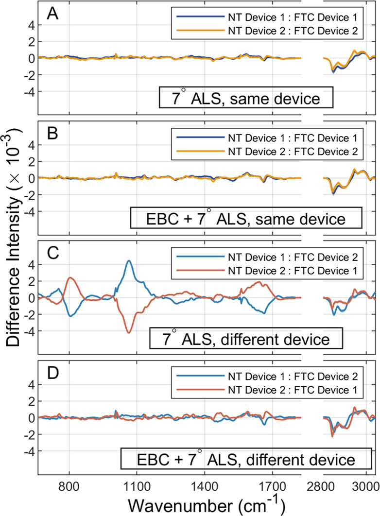
Spectral differences between NT and FTC with and without EBC. Difference spectra between NT and FTC using only 7° ALS are shown for (A) intra-device NT-FTC pairings and (B) inter-device NT-FTC pairings. Analogous difference spectra for NT-FTC pairings in which EBC was used prior to baseline correction are shown for (C) intra-device pairings and (D) inter-device pairings. In all panels, solid lines indicate median difference spectra and shading the IQR over 1000 resamples. The silent region, 1800–2800 cm–1, is replaced in all panels by a small vacancy. Note that FTC spectra are subtracted from NT spectra such that positive differences indicate larger NT intensity and negative differences indicate larger FTC intensity.
All difference spectra shown in Figure 2 indicate negative intensity differences that are comparable in magnitude to the average spectral intensity, near 2800–2900 cm–1, corresponding to a lower relative intensity of CH2 groups in lipids in FTC spectra. Intra-device differences in Figure 2A suggest that spectra from the same device are comparable using only ALS baseline correction, and Figure 2B indicates that the use of EBC has little effect on the intra-device difference as significant features that are present in Figure 2A are also present in Figure 2B. However, the inter-device differences in Figure 2C suggest that ALS baseline correction is insufficient when NT and FTC spectra originate from different devices as the largest differences in intensity (∼800, 1050, and 1600–1700 cm–1) arise from extrinsic sources and are as much as twice as large in magnitude as the average spectral intensity. In contrast, Figure 2D shows that these extrinsic contributions are not present when EBC is used. Though some small fluctuation between the devices remains, the significant features that appear in Figure 2A,B are preserved, and the extrinsic features observed in Figure 2C are reduced. Overall, Figure 2 suggests that the use of EBC is not only advantageous when spectra from different devices are used but are vital to spectral comparability across devices.
EBC Reduces False Discoveries Arising from Extrinsic Contributions
After confirming that the use of EBC is advantageous when the spectra originating from different devices are used, we demonstrate that machine learning models such as k-NN can learn extrinsic contributions and use them to return anomalously high classification accuracies. Figure 3 shows PC spaces and results of k-NN classifications for several different pairings. The first 2 dimensions of the PC projection of spectra that are not subject to EBC are shown in Figure 3A. Each spectrum is represented as a small circle; colors indicate the cell line and the device, as noted in Figure 3A,B. As suggested by the difference spectra in Figure 2B, device-based differences are more prominent than biological differences in the PC space as a significant overlap is observed between NT and FTC originating from a single device, but there are little overlap devices. In contrast, the use of EBC unifies the devices in the PC space of Figure 3B as spectra from the same cell line and different devices are overlapped. Both PC spaces show a significant overlap between NT and FTC spectra, suggesting that lower accuracy should be expected from a k-NN classification.
Figure 3.

k-NN classification of NT and FTC in the PC space with and without implementation of EBC. (A) PC space using only 7° ALS. (B) PC space when performing EBC prior to ALS. NT-FTC classification accuracies for a k-NN classification model using (C) the PC space without EBC (Figure 3A) and (D) the PC space with EBC (Figure 3B). Bar heights in (C) and (D) represent median accuracies over 1000 independent classifications (see Supporting Information, Section S2). Error bars in (C) and (D) indicate the accuracy extrema of each pairing. Labels within the bars of (C) and (D) indicate the particular NT:FTC device pairing. D1:D1 indicates NT Device 1: FTC Device 1 pairing, D2:D2 indicates NT Device 2 with FTC Device 2, D1:D2 the NT Device 1: FTC Device 2 pairing, and D2:D1 NT Device 2: FTC Device 1 pairing.
k-NN classifications were performed for discrimination of NT and FTC using all spectra and device-partitioned subsets (see Supporting Information, Section S1) that are indicated in Figure 3C,D using the notation NT Device: FTC Device. Note that horizontal axis labels of Figure 3C,D are abbreviated further; for example, D1:D2 indicates the pairing of NT Device 1 spectra with FTC Device 2 spectra. Classification for each NT-FTC pairing (All, D1:D1, D1:D2, D2:D1, D2:D2) was repeated 1000 times using randomly sampled subsets. Class sampling was balanced for each individual classification such that the baseline accuracy arising from a random classification is 50%. Accuracy is reported as the ratio of the number of correct classifications to the number of spectra in the test set. Bar heights in Figure 3C,D indicate the average accuracy obtained for each pairing, which are also displayed numerically above each bar. Error bars indicate the minimum and maximum accuracies obtained for that pairing.
Figure 3C displays accuracies obtained in cases that EBC was not used, while Figure 3D displays accuracies for cases in which EBC was implemented prior to ALS. Results showing the effects of EBC alone are included in Figure S3 (Supporting Information, Section S4). As shown in Figure 3C, relatively low accuracies near 70% are obtained for all spectra and the intra-device pairings, indicating poor discrimination of NT and FTC spectra by the model. However, accuracies are nearly perfect for inter-device pairings, suggesting that the k-NN model is learning and utilizing device-specific information to classify spectra as cancerous or not. In contrast, when EBC is used prior to ALS (Figure 3D), all accuracies are relatively and consistently low, between 67 and 79%, regardless of whether the pairing is intra-device, inter-device, or mixed.
The information that the models have learned is quantified with a post hoc analysis in which class spectra output from the k-NN classification models are used to gain information about the spectral features the models assign to the NT and FTC classes. Output class spectra are shown in Figures S4 and S5 (Supporting Information, Section S5) for classifications without and with the use of EBC, respectively. Figure 4 compares median difference spectra (solid) and the IQRs (shading) in which EBC was not (blue) or was (orange) used between the class spectra output by 1000 resampled k-NN models. Note that the spectrum assigned to the FTC class is subtracted from the spectrum assigned to the NT class, such that negative differences indicate higher intensity in the FTC class spectrum and positive difference indicates higher intensity in the NT class spectrum, as seen in Figure 2. Solid lines in Figure 4 represent the median difference spectrum and shaded regions the IQR. Each panel compares the difference spectra obtained from a unique NT-FTC pairing, with classification using all spectra shown in Figure 4A, intra-device pairings shown in Figure 4B,C, and finally inter-device pairings in Figure 4D,E.
Figure 4.

Post hoc difference spectra for k-NN classification models. Difference spectra obtained from the NT and FTC class spectra, as estimated by the k-NN models. The sets of spectra that are sampled for each panel are (A) all spectra, (B) NT Device 1 and FTC Device 1, (C) NT Device 2 and FTC Device 2, (D) NT Device 1 and FTC Device 2, (E) NT Device 2 and FTC Device 1. Solid lines indicate median difference spectra and shading the IQR over 1000 resamples. The silent region from 1800 to 2800 cm–1 has replaced with a small vacancy. Note FTC spectra are subtracted from NT spectra such that positive differences indicate larger NT intensity and negative differences indicate larger FTC intensity.
All panels of Figure 4 indicate negative difference intensity in the 2800–2900 cm–1 region, suggesting that the k-NN models associate higher intensity in this region with the FTC class (negative difference intensity), which was shown to be a true biological difference in Figures S2 and 2. While these are the only major features in the cases that EBC was used (orange color) and the intra-device classifications (Figure 4A,B), the classifications using all spectra and inter-device classifications, Figure 4A,D,E, respectively, all show nonzero intensities near 800 and 1050 cm–1, wavenumbers that are attributed to optical components. The difference near 800 cm–1 arising from optical components of Device 1 has large magnitude in the direction of the class originating from Device 1, positive in Figure 4D for NT Device 1: FTC Device 2 and negative for NT Device 2: FTC Device 1 in Figure 4E, suggesting that the k-NN model associates higher intensity at this feature with the class originating from Device 1. In a complementary manner, large magnitude is also observed near 1050 cm–1, arising from optics of Device 2. This difference intensity is negative for NT Device 1: FTC Device 2 (Figure 4D) and positive for NT Device 2: FTC Device 1 (Figure 4E), suggesting that the model associates higher intensity at this feature with the class originating from Device 2. Considering that the accuracies obtained for these classifications without EBC are larger than the intra-device classifications (see Figure 3C), it can be inferred that the k-NN model is using this extrinsic information to better distinguish the cell lines, particularly in the case of the inter-device classifications. This is obviously undesirable as this could lead to false discovery.
In contrast, the difference intensities at these wavenumbers when EBC was used are near zero, suggesting that the models do not associate intensity at these wavenumbers with a specific class. Additionally, the difference spectra for the inter-device pairings are similar to each other and to the intra-device pairings, suggesting that EBC is effective in reducing extrinsic contributions in the spectra. Furthermore, the post hoc difference spectra obtained from the k-NN classifications are similar to the intra-device difference spectra shown in Figure 2A,C, also suggesting that biological contents are retained after the use of EBC. Overall, Figure 4 shows that, while the k-NN models learn device-based effects, resulting in anomalously high accuracies when spectra from different devices are used, EBC can mitigate these extrinsic effects and allow the k-NN models to return consistent results regardless of the device from which the spectra originated.
EBC Used in Concert with Other Baseline Methods Reduces Device Recognition in Both Cell Lines
Because EBC focuses on those pixels containing the least amount of information about the sample of interest, intrinsic background signals such as autofluorescence should not be captured by EBC. Here, we use EBC in combination with other baseline methods to capture both extrinsic and intrinsic background. Each of the selected methods, ALS,24 recursive polynomial fitting (RPF),25 and rolling ball (RB)26 makes use of an adjustable parameter that controls the broadness in the wavenumber domain of the features that are allowed in the baseline estimate, with small radii (RB) and higher order polynomials (ALS and RPF), yielding baselines with broader features. Here, we adjust these parameters and assess the recognition of the device from which a particular spectrum originated using a k-NN classification model in the PC space, as was used above for recognition of disease states. In this approach, however, we wish to discriminate device rather than disease, so the k-NN models are trained with device labels instead of disease labels. Furthermore, each k-NN model is confined to a single cell line to avoid biological contamination. Models are trained to recognize the device both with and without EBC, which is applied prior to the use of the baseline method when it is used. For example, in the use of EBC with 7° ALS, EBC is applied first, and then each spectrum is corrected individually for baseline with 7° ALS. Spectra are transformed to the PC space for training and testing in the k-NN model. In cases that EBC is not used, that step in this procedure is simply skipped, and 7° ALS is applied directly to the raw spectra as in many standard preprocessing procedures.16,21 The value of EBC can thus be quantified through a decrease in the device-based accuracy returned by the k-NN model when it is used.
k-NN accuracies for device-based classification are shown in Figure 5 without the use of EBC for a range of different broadness parameters. Note that the broadness parameters, polynomial orders (ALS and RPF) and radius (RB) are arranged such that baseline estimates with broader (narrower) features lie to the left (right) of the panels. Figure 5A,B contains accuracies for ALS baseline models, Figure 5C,D contains RPF models, and Figure 5E,F contains RB models. k-NN models acting on spectra in which EBC was used are colored (blue for NT and red for FTC), while those acting on spectra in which EBC was not used are indicated in gray color. Figure 5 indicates that it is advantageous to correct for extrinsic background signal regardless of the choice of the baseline method and adjustable parameter as accuracies are decreased for all baseline methods and all choices of adjustable parameters used here when classification uses spectra after EBC. Device is readily recognized by the k-NN models when EBC is not used, returning accuracies for all methods and adjustable parameters of nearly 100%. When EBC is used, however, device-based recognition is reduced by up to 30%. This is advantageous in avoiding false discoveries arising from extrinsic sources that may contribute to distinction between, for example, cancerous and benign cell lines.
Figure 5.

k-NN device discrimination for different baseline correction methods with and without EBC. Device recognition by k-NN models is compared with (blue, red) and without (gray color) the use of EBC. Baseline correction was performed with ALS, RPF, and RB, and the feature broadness parameters were varied as indicated along the horizontal axes. Device-based k-NN classification was performed on spectra with ALS correction spectra for (A) NT and (B) FTC, RPF correction for (C) NT and (D) FTC, and RB correction for (E) NT and (F) FTC. Error bars over 1000 classifications are contained within the span of each marker.
Outlook
Through segmentation of the least intense group of pixels in a Raman microscopic image, we estimated background spectra arising from sources that are extrinsic to the sample of interest, such as the substrate and optical system. EBC was performed on a data set containing 50 experimental Raman images of in vitro cell cultures of 2 cell lines, the malignant RO 82 W-1 FTC cell line, and the benign Nthy-ori 3–1 follicular epithelial cell line. We found that the use of EBC retained the biological distinctions between malignant and benign spectra while reducing the potential for false distinction between the species, even when the spectra originate from different Raman devices.
Comparison of Raman spectra across different optical devices is known to be difficult,31,32 owing not just to extrinsic optical contributions to the spectra but other factors such as wavenumber drift, for which EBC alone is insufficient. This hinders the reproducibility of Raman microscopic experiments, limits the amount of data that can be included in a particular study, and thus limits the overall reliability and potential of Raman microscopy. This study, for example, was limited to two Raman devices and would benefit from further validation across many other devices as well as other cell lines having different spectral properties, although EBC was shown to be robust against variation in spectral shape on synthetic data (Supporting Information, Section S6). The viability of EBC may be hindered in some situations, such as samples in which the background spectrum is not uniform across the sample. In these cases, EBC can be adapted to estimate a local background spectrum, either by modifying pixel segmentation to, for example, operate over local regions of the image, or by adopting a nearest-neighbors-type calculation with segmented background pixels. EBC relies on the presence of pixels in which the intensity from the sample of interest approaches zero; in samples with very dense signal such as biological tissues, EBC may be hindered by the absence of background pixels, causing the background estimate to include contribution from the sample. The behavior of EBC in such a situation is a possible route of further study. EBC may also affect the behavior of components that are present in the sample medium, such as water. In this case, the spectra corrected with EBC will show intensity relative to the intensity of the particular component in the medium. For example, regions that are less rich in water than the sample medium will produce negative intensity from 3100 to 3600 after EBC. EBC may also be useful in other applications. Recent examples38 of standardization of Raman spectra across multiple devices use transfer learning to adjust for device-specific differences, a scheme in which the use of an extrinsic background spectrum may be advantageous. Finally, pixel segmentation relies on a 1-D set of intensities that are assumed to be sampled from some mixture of Poisson distributions, making EBC suitable for locating the darkest set of intensities in any set of photon-counting data, regardless of its origin. Due to its adaptability and ability to adjust for variability in extrinsic contributions across different devices, experimental instances, and images, we expect EBC to be of great utility in and beyond the Raman microscopy community.
Acknowledgments
We thank Atsuyoshi Nakamura, Koji Tabata, and Khalifa Helal for important discussions during this research. This work was partially supported by AIST-Osaka University Advanced Photonics and Biosensing Open Innovation Laboratory (PhotoBio-OIL), Japan Science and Technology Agency (JST) COI-NEXT Grant Number JPMJPF2009, Japan Society for the Promotion of Science (JSPS), Grant-in-Aid for Scientific Research (No. 25287105) (to T.K.), Grant-in-Aid for Exploratory Research (No. 25650044) (to T.K.), JST Core Research for Evolutional Science and Technology (CREST), Grant Number JPMJCR1662, Japan (to T.K., K.F., Y.H.), and the Research Program of “Dynamic Alliance for Open Innovation Bridging Human, Environment and Materials” in ″Network Joint Re-search Center for Materials and Devices″ (to Y.H.).
Supporting Information Available
The Supporting Information is available free of charge at https://pubs.acs.org/doi/10.1021/acs.analchem.3c01406.
Device specifications and supplementary methods; background pixel mappings for all 50 experimental images; NT and FTC spectral comparison among devices; PC space and k-NN models for EBC without the use of ALS; NT and FTC class spectra output by the k-NN models; and spectral recovery with EBC using synthetic Raman images (PDF)
Author Contributions
J.N.T. conceived EBC with advice from T.K and A.P. J.N.T., K.F., T.B., A.P., and T.K. wrote the manuscript. K.M., K.H., and Y.K. performed Raman measurements. Y.H., Y.K, and K.F. supervised the Raman measurements. J.N.T. performed all computations. T.K., K.F., and Y.H. secured funding for this research.
The authors declare no competing financial interest.
Notes
EBC software implementation is available at https://github.com/haarlet/ebc.
Supplementary Material
References
- Pandey R.; Paidi S. K.; Valdez T. A.; Zhang C.; Spegazzini N.; Dasari R. R.; Barman I. Noninvasive Monitoring of Blood Glucose with Raman Spectroscopy. Acc. Chem. Res. 2017, 50, 264–272. 10.1021/acs.accounts.6b00472. [DOI] [PMC free article] [PubMed] [Google Scholar]
- Kloß S.; Kampe B.; Sachse S.; Rösch P.; Straube E.; Pfister W.; Kiehntopf M.; Popp J. Culture Independent Raman Spectroscopic Identification of Urinary Tract Infection Pathogens: A Proof of Principle Study. Anal. Chem. 2013, 85, 9610–9616. 10.1021/ac401806f. [DOI] [PubMed] [Google Scholar]
- Dies H.; Raveendran J.; Escobedo C.; Docoslis A. Rapid Identification and Quantification of Illicit Drugs on Nanodendritic Surface-Enhanced Raman Scattering Substrates. Sens. Actuators, B 2018, 257, 382–388. 10.1016/j.snb.2017.10.181. [DOI] [Google Scholar]
- Khandasammy S. R.; Fikiet M. A.; Mistek E.; Ahmed Y.; Halámková L.; Bueno J.; Lednev I. K. Bloodstains, Paintings, and Drugs: Raman Spectroscopy Applications in Forensic Science. Forensic Chem. 2018, 8, 111–133. 10.1016/j.forc.2018.02.002. [DOI] [PubMed] [Google Scholar]
- Peizhen X.; Bowen C.; Yeqiang B.; Hongtao W.; Xin G.; Pan W.; Ron S. Y.; Limin T. Elastic Ice Microfibers. Science 2021, 373, 187–192. 10.1126/science.abh3754. [DOI] [PubMed] [Google Scholar]
- Antonio K. A.; Schultz Z. D. Advances in Biomedical Raman Microscopy. Anal. Chem. 2014, 86, 30–46. 10.1021/ac403640f. [DOI] [PubMed] [Google Scholar]
- Hill A. H.; Fu D. Cellular Imaging Using Stimulated Raman Scattering Microscopy. Anal. Chem. 2019, 91, 9333–9342. 10.1021/acs.analchem.9b02095. [DOI] [PubMed] [Google Scholar]
- Butler H. J.; Ashton L.; Bird B.; Cinque G.; Curtis K.; Dorney J.; Esmonde-White K.; Fullwood N. J.; Gardner B.; Martin-Hirsch P. L.; Walsh M. J.; McAinsh M. R.; Stone N.; Martin F. L. Using Raman Spectroscopy to Characterize Biological Materials. Nat. Protoc. 2016, 11, 664–687. 10.1038/nprot.2016.036. [DOI] [PubMed] [Google Scholar]
- Palonpon A. F.; Ando J.; Yamakoshi H.; Dodo K.; Sodeoka M.; Kawata S.; Fujita K. Raman and SERS Microscopy for Molecular Imaging of Live Cells. Nat. Protoc. 2013, 8, 677–692. 10.1038/nprot.2013.030. [DOI] [PubMed] [Google Scholar]
- Takeuchi M.; Kajimoto S.; Nakabayashi T. Experimental Evaluation of the Density of Water in a Cell by Raman Microscopy. J. Phys. Chem. Lett. 2017, 8, 5241–5245. 10.1021/acs.jpclett.7b02154. [DOI] [PubMed] [Google Scholar]
- Adamczyk A.; Matuszyk E.; Radwan B.; Rocchetti S.; Chlopicki S.; Baranska M. Toward Raman Subcellular Imaging of Endothelial Dysfunction. J. Med. Chem. 2021, 64, 4396–4409. 10.1021/acs.jmedchem.1c00051. [DOI] [PMC free article] [PubMed] [Google Scholar]
- Belanger M. C.; Anbaei P.; Dunn A. F.; Kinman A. W. L.; Pompano R. R. Spatially Resolved Analytical Chemistry in Intact, Living Tissues. Anal. Chem. 2020, 92, 15255–15262. 10.1021/acs.analchem.0c03625. [DOI] [PMC free article] [PubMed] [Google Scholar]
- Helal K. M.; Taylor J. N.; Cahyadi H.; Okajima A.; Tabata K.; Itoh Y.; Tanaka H.; Fujita K.; Harada Y.; Komatsuzaki T. Raman Spectroscopic Histology Using Machine Learning for Nonalcoholic Fatty Liver Disease. FEBS Lett. 2019, 593, 2535–2544. 10.1002/1873-3468.13520. [DOI] [PubMed] [Google Scholar]
- Nishiki-Muranishi K.; Harada Y.; Minamikawa T.; Yamaoka Y.; Dai P.; Yaku H.; Takamatsu T. Label-Free Evaluation of Myocardial Infarction and Its Repair by Spontaneous Raman Spectroscopy. Anal. Chem. 2014, 86, 6903–6910. 10.1021/ac500592y. [DOI] [PubMed] [Google Scholar]
- Ji-Xin C.; Xie X. S. Vibrational Spectroscopic Imaging of Living Systems: An Emerging Platform for Biology and Medicine. Science 2015, 350, aaa8870 10.1126/science.aaa8870. [DOI] [PubMed] [Google Scholar]
- Bocklitz T. W.; Guo S.; Ryabchykov O.; Vogler N.; Popp J. Raman Based Molecular Imaging and Analytics: A Magic Bullet for Biomedical Applications!?. Anal. Chem. 2016, 88, 133–151. 10.1021/acs.analchem.5b04665. [DOI] [PubMed] [Google Scholar]
- Lussier F.; Thibault V.; Charron B.; Wallace G. Q.; Masson J.-F. Deep Learning and Artificial Intelligence Methods for Raman and Surface-Enhanced Raman Scattering. Trends Analyt. Chem. 2020, 124, 115796 10.1016/j.trac.2019.115796. [DOI] [Google Scholar]
- Guo S.; Popp J.; Bocklitz T. Chemometric Analysis in Raman Spectroscopy from Experimental Design to Machine Learning–Based Modeling. Nat. Protoc. 2021, 16, 5426–5459. 10.1038/s41596-021-00620-3. [DOI] [PubMed] [Google Scholar]
- Brownfield B.; Lemos T.; Kalivas J. H. Consensus Classification Using Non-Optimized Classifiers. Anal. Chem. 2018, 90, 4429–4437. 10.1021/acs.analchem.7b04399. [DOI] [PubMed] [Google Scholar]
- Kang S.; Kim I.; Vikesland P. J. Discriminatory Detection of ssDNA by Surface-Enhanced Raman Spectroscopy (SERS) and Tree-Based Support Vector Machine (Tr-SVM). Anal. Chem. 2021, 93, 9319–9328. 10.1021/acs.analchem.0c04576. [DOI] [PubMed] [Google Scholar]
- Taylor J. N.; Mochizuki K.; Hashimoto K.; Kumamoto Y.; Harada Y.; Fujita K.; Komatsuzaki T. High-Resolution Raman Microscopic Detection of Follicular Thyroid Cancer Cells with Unsupervised Machine Learning. J. Phys. Chem. B 2019, 123, 4358–4372. 10.1021/acs.jpcb.9b01159. [DOI] [PubMed] [Google Scholar]
- Kang S.; Nam W.; Zhou W.; Kim I.; Vikesland P. J. Nanostructured Au-Based Surface-Enhanced Raman Scattering Substrates and Multivariate Regression for PH Sensing. ACS Appl. Nano Mater. 2021, 4, 5768–5777. 10.1021/acsanm.1c00549. [DOI] [Google Scholar]
- Zhang S.; Song Z.; Godaliyadda G. M. D. P.; Ye D. H.; Chowdhury A. U.; Sengupta A.; Buzzard G. T.; Bouman C. A.; Simpson G. J. Dynamic Sparse Sampling for Confocal Raman Microscopy. Anal. Chem. 2018, 90, 4461–4469. 10.1021/acs.analchem.7b04749. [DOI] [PMC free article] [PubMed] [Google Scholar]
- Mazet V.; Carteret C.; Brie D.; Idier J.; Humbert B. Background Removal from Spectra by Designing and Minimising a Non-Quadratic Cost Function. Chemom. Intell. Lab. Syst. 2005, 76, 121–133. 10.1016/j.chemolab.2004.10.003. [DOI] [Google Scholar]
- Lieber C. A.; Mahadevan-Jansen A. Automated Method for Subtraction of Fluorescence from Biological Raman Spectra. Appl. Spectrosc. 2003, 57, 1363–1367. 10.1366/000370203322554518. [DOI] [PubMed] [Google Scholar]
- Kneen M. A.; Annegarn H. J. Algorithm for Fitting XRF, SEM and PIXE X-Ray Spectra Backgrounds. Nucl. Instrum. Methods Phys. Res., Sect. B 1996, 109–110, 209–213. 10.1016/0168-583X(95)00908-6. [DOI] [Google Scholar]
- Perez-Pueyo R.; Soneira M. J.; Ruiz-Moreno S. Morphology-Based Automated Baseline Removal for Raman Spectra of Artistic Pigments. Appl. Spectrosc. 2010, 64, 595–600. 10.1366/000370210791414281. [DOI] [PubMed] [Google Scholar]
- Li H.; Dai J.; Pan T.; Chang C.; So H. C. Sparse Bayesian Learning Approach for Baseline Correction. Chemom. Intell. Lab. Syst. 2020, 204, 104088 10.1016/j.chemolab.2020.104088. [DOI] [Google Scholar]
- de Rooi J. J.; Eilers P. H. C. Mixture Models for Baseline Estimation. Chemom. Intell. Lab. Syst. 2012, 117, 56–60. 10.1016/j.chemolab.2011.11.001. [DOI] [Google Scholar]
- Guo S.; Bocklitz T.; Popp J. Optimization of Raman-Spectrum Baseline Correction in Biological Application. Analyst 2016, 141, 2396–2404. 10.1039/C6AN00041J. [DOI] [PubMed] [Google Scholar]
- Liland K. H.; Almøy T.; Mevik B.-H. Optimal Choice of Baseline Correction for Multivariate Calibration of Spectra. Appl. Spectrosc. 2010, 64, 1007–1016. 10.1366/000370210792434350. [DOI] [PubMed] [Google Scholar]
- Dörfer T.; Bocklitz T.; Tarcea N.; Schmitt M.; Popp J. Checking and Improving Calibration of Raman Spectra Using Chemometric Approaches. Z. Phys. Chem. 2011, 225, 753–764. 10.1524/zpch.2011.0077. [DOI] [Google Scholar]
- Guo S.; Beleites C.; Neugebauer U.; Abalde-Cela S.; Afseth N. K.; Alsamad F.; Anand S.; Araujo-Andrade C.; Aškrabić S.; Avci E.; Baia M.; Baranska M.; Baria E.; Batista de Carvalho L. A. E.; de Bettignies P.; Bonifacio A.; Bonnier F.; Brauchle E. M.; Byrne H. J.; Chourpa I.; Cicchi R.; Cuisinier F.; Culha M.; Dahms M.; David C.; Duponchel L.; Duraipandian S.; El-Mashtoly S. F.; Ellis D. I.; Eppe G.; Falgayrac G.; Gamulin O.; Gardner B.; Gardner P.; Gerwert K.; Giamarellos-Bourboulis E. J.; Gizurarson S.; Gnyba M.; Goodacre R.; Grysan P.; Guntinas-Lichius O.; Helgadottir H.; Grošev V. M.; Kendall C.; Kiselev R.; Kölbach M.; Krafft C.; Krishnamoorthy S.; Kubryck P.; Lendl B.; Loza-Alvarez P.; Lyng F. M.; Machill S.; Malherbe C.; Marro M.; Marques M. P. M.; Matuszyk E.; Morasso C. F.; Moreau M.; Muhamadali H.; Mussi V.; Notingher I.; Pacia M. Z.; Pavone F. S.; Penel G.; Petersen D.; Piot O.; Rau J. V.; Richter M.; Rybarczyk M. K.; Salehi H.; Schenke-Layland K.; Schlücker S.; Schosserer M.; Schütze K.; Sergo V.; Sinjab F.; Smulko J.; Sockalingum G. D.; Stiebing C.; Stone N.; Untereiner V.; Vanna R.; Wieland K.; Popp J.; Bocklitz T. Comparability of Raman Spectroscopic Configurations: A Large Scale Cross-Laboratory Study. Anal. Chem. 2020, 92, 15745–15756. 10.1021/acs.analchem.0c02696. [DOI] [PubMed] [Google Scholar]
- Hutsebaut D.; Vandenabeele P.; Moens L. Evaluation of an Accurate Calibration and Spectral Standardization Procedure for Raman Spectroscopy. Analyst 2005, 130, 1204–1214. 10.1039/B503624K. [DOI] [PubMed] [Google Scholar]
- Chen H.; Zhang Z.-M.; Miao L.; Zhan D.-J.; Zheng Y.-B.; Liu Y.; Lu F.; Liang Y.-Z. Automatic Standardization Method for Raman Spectrometers with Applications to Pharmaceuticals. J. Raman Spectrosc. 2015, 46, 147–154. 10.1002/jrs.4602. [DOI] [Google Scholar]
- Rodriguez J. D.; Westenberger B. J.; Buhse L. F.; Kauffman J. F. Standardization of Raman Spectra for Transfer of Spectral Libraries across Different Instruments. Analyst 2011, 136, 4232–4240. 10.1039/C1AN15636E. [DOI] [PubMed] [Google Scholar]
- Afseth N. K.; Kohler A. Extended Multiplicative Signal Correction in Vibrational Spectroscopy, a Tutorial. Chemom. Intell. Lab. Syst. 2012, 117, 92–99. 10.1016/j.chemolab.2012.03.004. [DOI] [Google Scholar]
- Guo S.; Kohler A.; Zimmermann B.; Heinke R.; Stöckel S.; Rösch P.; Popp J.; Bocklitz T. Extended Multiplicative Signal Correction Based Model Transfer for Raman Spectroscopy in Biological Applications. Anal. Chem. 2018, 90, 9787–9795. 10.1021/acs.analchem.8b01536. [DOI] [PubMed] [Google Scholar]
- Stauffer C.; Grimson W. E. L.. Adaptive Background Mixture Models for Real-Time Tracking. In Proceedings 1999 IEEE Computer Society Conference on Computer Vision and Pattern Recognition (Cat. No PR00149); IEEE, 1999; Vol. 2, pp 246–252. [Google Scholar]
- Deng T.; DePaoli D.; Bégin L.; Jia N.; Torres de Oliveira L.; Côté D. C.; Vincent W. F.; Greener J. Versatile Microfluidic Platform for Automated Live-Cell Hyperspectral Imaging Applied to Cold Climate Cyanobacterial Biofilms. Anal. Chem. 2021, 93, 8764–8773. 10.1021/acs.analchem.0c05446. [DOI] [PubMed] [Google Scholar]
- Al-Zubeidi A.; Stein F.; Flatebo C.; Rehbock C.; Hosseini Jebeli S. A.; Landes C. F.; Barcikowski S.; Link S. Single-Particle Hyperspectral Imaging Reveals Kinetics of Silver Ion Leaching from Alloy Nanoparticles. ACS Nano 2021, 15, 8363–8375. 10.1021/acsnano.0c10150. [DOI] [PubMed] [Google Scholar]
- Veirs D. K.; Ager J. W.; Loucks E. T.; Rosenblatt G. M. Mapping Materials Properties with Raman Spectroscopy Utilizing a 2-D Detector. Appl. Opt. 1990, 29, 4969–4980. 10.1364/AO.29.004969. [DOI] [PubMed] [Google Scholar]
- Hamada K.; Fujita K.; Smith N. I.; Kobayashi M.; Inouye Y.; Kawata S. Raman Microscopy for Dynamic Molecular Imaging of Living Cells. J. Biomed. Optics 2008, 13, 1–4. 10.1117/1.2952192. [DOI] [PubMed] [Google Scholar]
Associated Data
This section collects any data citations, data availability statements, or supplementary materials included in this article.