Mapping the Impact of Approximate Gradient Nonlinearity Fields Correction on Tractography

Abstract

Nonlinear gradients impact diffusion weighted MRI by introducing spatial variation in estimated diffusion tensors. Recent studies have shown that increasing signal-to-noise ratios and the use of ultra-strong gradients may lead to clinically significant impacts on analyses due to these nonlinear gradients in microstructural measures. These effects can potentially bias tractography results and cause misinterpretation of data. Herein, we characterize the impact of an “approximate” gradient nonlinearity correction technique in tractography using empirically derived gradient nonlinear fields. This technique scales the diffusion signal by the change in magnitude due to the gradient nonlinearities, without concomitant correction of gradient direction errors. The impact of this correction on tractography is assessed through white matter bundle segmentation and connectomics via bundle-wise volume, fractional anisotropy, mean diffusivity, radial diffusivity, axial diffusivity, primary eigenvector, and length; as well as the modularity, global efficiency, and characteristic path length connectomics graph measures. We investigate the differences between (1) these measures directly and (2) the within session variability of these measures before and after approximate correction in 61 subjects from the MASiVar pediatric reproducibility dataset. We find approximate correction results is little to no differences on the population level, but large differences on the subject-specific level for both the measures directly and their within session variability. Thus, this study suggests though approximate correction of gradient nonlinearities may not change tractography findings on the population level, subject-specific interpretations may exhibit large fluctuations. A limitation is the lack of comparison with the empirical voxel-wise gradient table correction.

INTRODUCTION

Diffusion weighted magnetic resonance imaging (DW-MRI) tractography provides an in-vivo mapping of the structural connectivity of the brain by estimating microstructural quantities [1]. Tractography is often used in neurological research studies and clinical studies to associate disease and white matter (WM) connections [2–5]. Although DW-MRI is a widely used non-invasive technique, it is susceptible to various distortions due to the underlying physics [6]. One such distortion is from nonlinearities produced when the gradient fields are nonuniform in the diffusion volume leading to changes in magnitude and spatial orientation of the gradients [7]. Gradient nonlinearities cause incorrect estimations of the microstructure and may bias fiber tractography [8, 9]. These effects vary significantly between MRI scanners based on the manufacturing process and are more pronounced further away from the isocenter [10, 11].

Gradient nonlinearity correction may be performed either with manufacturer-specified gradient coil configurations or phantom study estimates of these scanner-specific gradient nonlinearities [12–14]. Several frameworks have been proposed to account for the nonlinear gradient coils including computing the spatially varying gradient coil L(r) that relates the intended and achieved gradient tables [10], rotation of the gradient nonlinearity tensor L(r) into the diffusion gradient frame [11], and velocity reconstruction using matrix formalization [15]. The effects of gradient nonlinearity correction in DW-MRI have been investigated and estimated to improve accuracy within and across sites and scanners [16, 17]. Studies show bias up to 30% in diffusion tensor information (DTI) [18], up to 10% in diffusion kurtosis imaging [8] and a direct effect on fiber orientation [9] when neglecting gradient nonlinearities. The errors from gradient nonlinearities depend on complex interactions, including motion [18], orientation and magnitude of gradients, underlying microstructure [19], signal-to-noise ratio (SNR), and diffusion weighting [8, 9].

The widely used empirical nonlinear gradient correction using local annotation of gradient magnitude and vectors and is expensive in terms of computation [10, 14]. Thus, we investigate and evaluate a simpler approach based on scaling the magnitude [8, 20]. We call this “approximate correction”. The approximate correction directly scales the DW-MRI signal equivalent to the change in magnitude and ignores the angular deviations [20]. Recently, with the increase in the use of the Connectome scanner with higher gradient strength of 300mT/m [21, 22] for better understanding of the brain’s microstructure, nonlinearities may increase, and thus it becomes vital to assess this correction approach in tractography (Figure 1).

Figure 1.

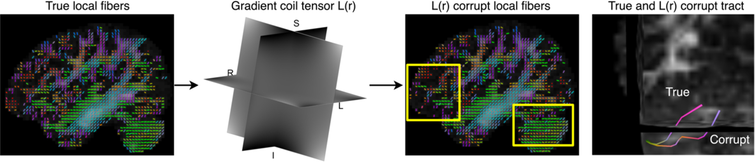
In DW-MRI, which uses magnetic field gradients to encode the diffusion signal, gradient nonlinearities cause spatial variations in the diffusion gradients. Tractography results can change depending on the spatial effects of nonlinear gradients which can cause the tracts to deviate to a false tract pathway. After initialization in tractography, when errors accumulate, a small change can result in a different streamline.

In this paper, we demonstrate the effects of approximate L(r) correction on probabilistic fiber tractography on a population of DW-MRI data by presenting connectome and bundle segmentation measures with and without applying approximate correction. Furthermore, we map the differences in reproducibility of these measures after nonlinearity correction.

METHODS

1.1. Data Overview

For this study, the publicly available MASiVar dataset (Cohort IV) was used [23]. Cohort IV consists of 83 healthy child subjects with ages 5–8 years. It has 48 male and 35 female participants scanned for one to two sessions on 3T Philips Achieva scanner (gradient strength of 80 mT/m and 200 T/m/s slew-rate). The imaging sessions were spaced approximately 1 year apart. Each scan within a session had a rescan and consists of a 40-direction b=1000 s/mm² and a 56-direction b=2000 s/mm² acquisition [23]. These scans were acquired at resolution of 2.1 × 2.1 × 2.2 mm and TE/TR of 79ms/2900ms. All subjects are processed with the tractography pipeline described in the next section (Figure 2). Tractography pipelines are fundamentally subjected to pitfalls [24] that lead to missing streamlines and missing bundles reconstruction. Subjects with more than 4 out of 39 bundles missing were considered as failed. Thus, there were 61 subjects that successfully passed the bundle reconstruction criteria. Within these subjects, there were 18 subjects with two sessions and 43 subjects with 1 session. Thus, there were 79 within session observations. The empirical field maps were estimated from the same scanner with 24 L synthetic white oil phantom in a polypropylene carboy with an approximate diameter of 290 mm and height of 50 mm [14, 25]. These field maps were previously reported [14]. The gradient coil tensor L(r) was generated with the field maps from the empirical field mapping procedure as described by Rogers et al. [12]. The L(r) tensor related the achieved magnetic gradient to the intended one.

Figure 2.

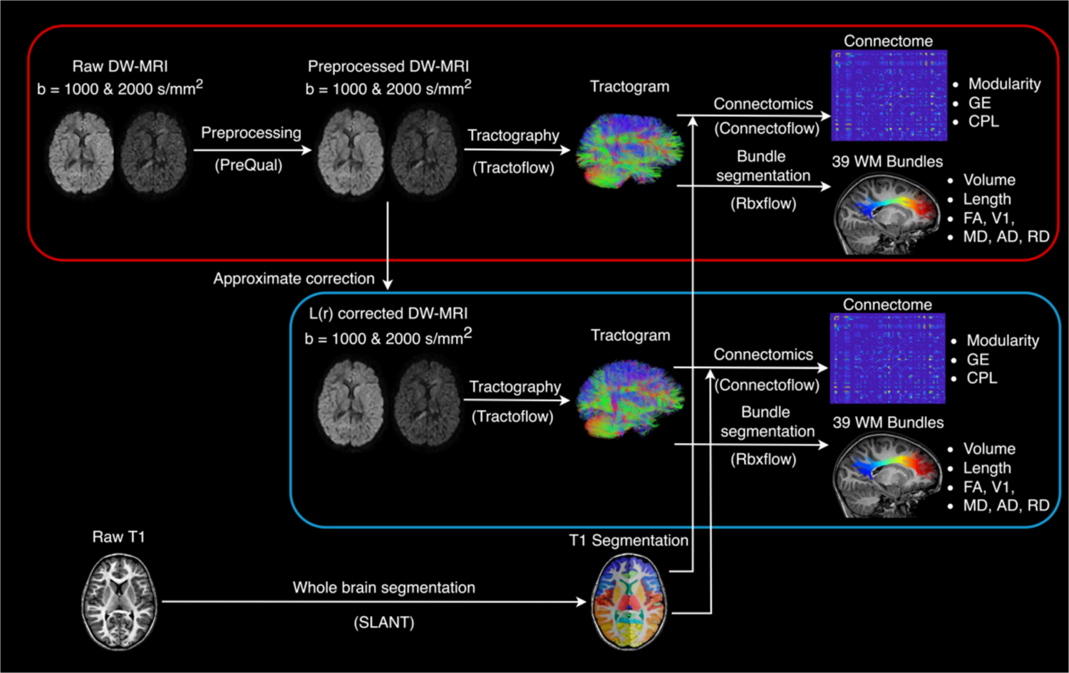
Outline of the processing pipeline with the measurements investigated for without (red block) and with (blue block) approximate L(r) correction. The raw DW-MRI data was preprocessed with PreQual. Approximate L(r) correction was applied to the preprocessed data. The tractography pipeline was performed on preprocessed data with and without L(r) correction. Bundle statistics and graph theory measures were evaluated from bundle segmentation and connectomes.

1.2. Preprocessing and approximate gradient nonlinearity correction

The raw DW-MRI are preprocessed and quality assured (QA) with the PreQual pipeline [26]. In the PreQual pipeline, denoising, intensity normalization, susceptibility-correction, eddy current-correction, motion-induced artifact correction, and slice-wise imputation of raw DW-MRI was executed. The preprocessed DW-MRI is corrected for nonlinear gradient distortion with an approximate correction technique [20]. The approximate correction involves the correction of magnitude. The actual gradient g′ were calculated by [14]

$$g^{\prime }=Lg$$ (1)

where g is the intended gradient and L is the gradient coil tensor. The achieved b-value b′ was then computed by adjusting the intended b-value, b by the square of the length change.

$$b^{\prime }=b{\left|g^{\prime }\right|}^2$$ (2)

Then, we approximate the effect of L(r) for a signal S_i in the i^th diffusion acquisition as

$$S_i\cong S_o{e}^{-b{\left|g^{\prime }\right|}^2{g}_i^{T}D{g}_i}$$ (3)

which further simplified to,

$$S_{\mathit{\text{approx}}}=S_o{e}^{\frac{\mathit{\text{ln}}\frac{S_i}{S_o}}{{\left|g^{\prime }\right|}^2}}$$ (4)

Thus, the approximate correction approach involved computing the corrected signal S_approx (Eq. (4)) by scaling the raw signal S_i with the square of the length change in (1). This is numerically equivalent to changing the b-value (which is shown in (Eq. 2)). This approach takes into account the magnitude component of deviations in actual and desired gradient amplitudes.

Tractography was performed on the preprocessed DW-MRI with and without approximate L(r) correction to assist the impact of approximate correction on tractography measures. The tractography pipeline consists of three parts 1) TractoFlow [27] produced a whole-brain probabilistic tractography and diffusion tensor information (DTI) and fiber orientation distribution function metrics using constrained spherical deconvolution (CSD), 2) ConnectoFlow [28] produced structural connectivity matrices weighted by connection-wise metrics reconstructed from a 125 region cortical parcellation produced by SLANT [29] and the tractograms from TractoFlow, and 3) RbxFlow [24] (RecobundlesX) performed segmentation of 39 major well-known WM pathways with a multi-atlas, multi-parameter approach based on Recobundles [30].

1.3. Graph theory measures and bundle segmentation measures

The connectivity matrices weighted by number of streamlines and average connection length from ConnectoFlow were used for the connectome analysis. These matrices are represented with graph-based measures. The graph theory measures were computed using the Brain Connectivity Toolbox (BCT) developed by Rubinov and Sporns for complex network analysis [31]. We evaluate the impact of L(r) correction on three graph-based measures namely: modularity, global efficiency, and characteristic path length (CPL). Modularity and global efficiency used matrices weighted by streamline count and CPL used the pseudo-length of matrices weighted by average length. Global efficiency was normalized between 0 and 1 as recommended by BCT [31].

The TractometryFlow [32] pipeline quantifies bundle-specific information by combining WM bundles from RbxFlow and DTI metrics. We acquire the bundle-wise mean length and volume. For bundle-wise DTI metrics, a binary bundle mask was calculated by thresholding the tract density image at 5% of the 99^th percentile density [23]. The median voxel-wise DTI metric is obtained with each bundle’s mask. Thus, we evaluate the impact of L(r) correction with bundle wise mean length, volume, fractional anisotropy (FA), mean diffusivity (MD), radial diffusivity (RD), axial diffusivity (AD) and principal eigenvector (V1).

1.4. Evaluation metric

We compute variability for scan-rescan images within a session with the coefficient of variation (CoV). CoV is defined as the standard deviation of scalar metrics within a session, σ, divided by the mean of scalar metrics within a session, $\overline{x}$, times 100%:

$$\mathit{\text{CoV}}(\%)=\frac{\sigma }{\overline{x}}\times 100\%$$ (5)

We compute residual change with absolute percent error (APE) (%) for scalar metrics and angular error (AE) (°) for V1. APE is defined as difference between the observed scalar metrics (here, the metrics before and after L(r) correction) divided by the true scalar metric (here, the metric before L(r) correction) times 100 %.

$$\mathit{\text{APE}}(\%)=\left|\frac{M_{\mathit{\text{corr}}}-M_{\mathit{\text{uncorr}}}}{M_{\mathit{\text{uncorr}}}}\right|\times 100\%$$ (6)

where M is the scalar metric, either modularity, global efficiency, CPL, mean length, volume, FA, MD, AD, or RD. Angular error (AE) (°) is defined as average angle between not applying and applying L(r) correction in V1. We compute the chord length C as follows,

$$C\left(V{1}_{\mathit{\text{corr}}},V{1}_{\mathit{\text{uncorr}}}\right)=\sqrt{\sum _{i=1}^n{\left(V{1}_{{\mathit{\text{corr}}}_i}-V{1}_{{\mathit{\text{uncorr}}}_i}\right)}^2}$$ (7)

Then the angle is evaluated as,

$$AE=2\times \text{arcsin}\frac{C}{2}$$ (8)

where V1_corr and V1_uncorr denote without and with L(r) correction. As the principal eigenvectors are sign agnostic, differences greater than π/2 radians are reoriented by multiplication by −1 such that the angle is ≤ π/2 [33, 34]. APE and AE was computed voxel-wise.

RESULTS

2.1. Effects of approximate correction of nonlinear fields on graph measures

Figure 3 shows the impact of L(r) correction on the connectomes’ measures directly (Figure 3a) and the within session variability of these measures (Figure 3b). For the impact on the connectomes’ measures directly (Figure 3a), we find that the median APE in modularity was 0.973%, in global efficiency was 3.4%, and in CPL was 0.48% for one scan from one session in 61 subjects. We also observe there are 9 subjects for modularity, 2 for global efficiency and 1 for CPL that experience a larger impact due to L(r) correction compared to the rest of the population (Figure 3a black dots). A negative difference of CoV indicate that the correction decreased the variability of the computed measure; this suggest that the computed measure for these subjects improved after L(r) correction, whereas a positive difference suggest the opposite effect. For within session variability (Figure 3b), we observe that the median difference in CoV before and after L(r) correction was 0.05% for modularity, −0.2% for global efficiency, and −0.09%. There are 5 subjects for modularity, 4 for global efficiency, and 2 for CPL that have a negative difference while 5 for modularity and 1 for global efficiency have a positive difference (Figure 3b black dots). Again, this denotes the subjects with negative difference improved after L(r) correction and the ones with positive difference has an opposite effect. This suggest that subjects are impacted differently, some exhibit large changes (Figure 3 back dots) while most others exhibit a smaller change. Since, there are more subjects with a smaller impact, we observe the median is close 0 at population level.

Figure 3.

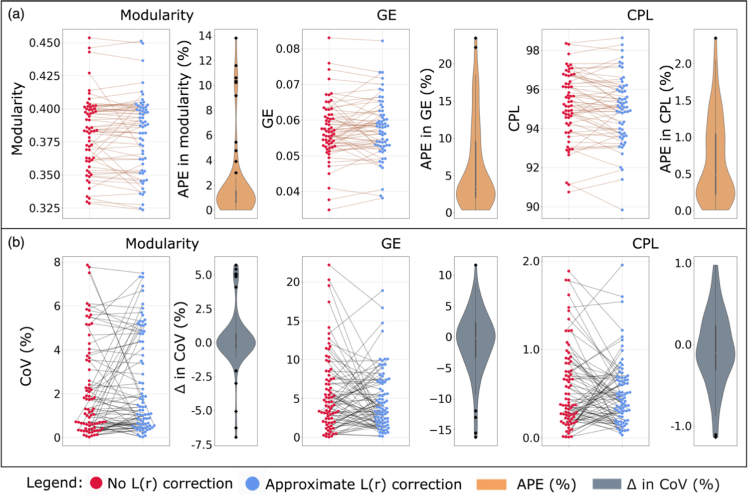
Effects of L(r) correction on (a) the graph measures and (b) the within session variability of graph measures. (a) Each data point was computed measure for a scan from a session in a subject with no correction (red dots) and approximate correction (blue dots). The data points from the same subjects are connected (brown lines) and the distribution of the APE in the data points connected was shown in brown. Notice, some subjects have a large effect (black dots). (b) Each data point was CoV of the computed measure for a within session observation with no correction (red dots) and approximate correction (blue dots). The data points from the same within session observations are connected (black lines) and the distribution of the difference in the data points connected was shown in grey. Again, some subjects have a large effect (black dots). The graphing tool range was limited within the range of the observed data. Abbreviations: CoV, coefficient of variation, GE, global efficiency, APE, absolute percent error, and CPL, characteristic path length.

In support with these findings, we observe larger changes in the 5^th and 90^th percentile differences in the connectivity matrices after L(r) correction across 61 subjects when compared to that of the 25^th and 75^th percentile (Figure 4). This suggest that the edges in the connectivity matrices for the middle 50% of subjects exhibit small changes while a portion of individuals exhibit dramatic changes.

Figure 4.

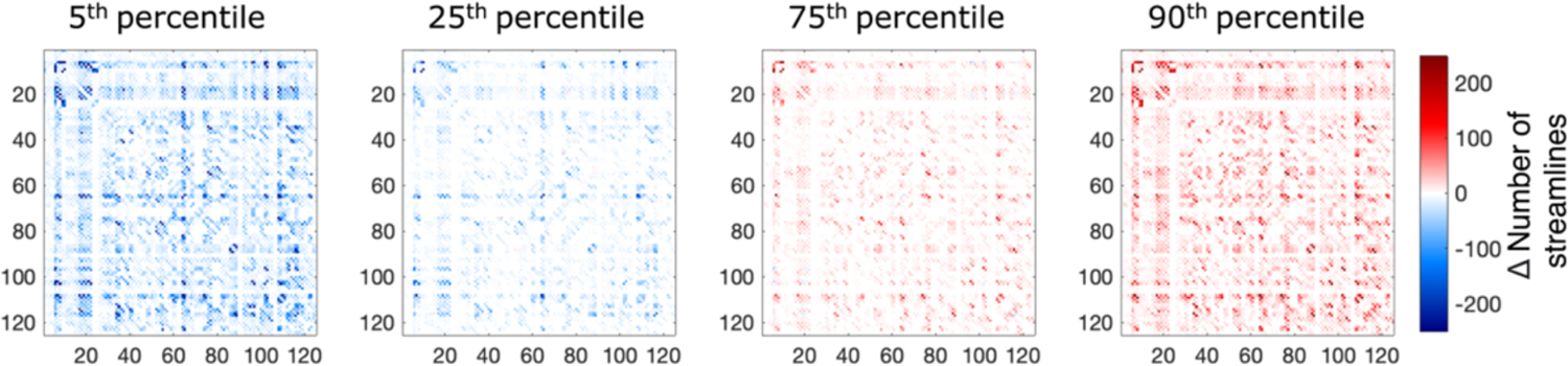
5^th, 25^th, 75^th, and 90^th percentile differences before and after approximate L(r) correction of connectivity matrices weighted by streamline count across 61 subjects. 5^th and 90^th percentile have larger changes in the edges up to 200 number of streamlines when compared 25^th and 75^th percentile.

2.2. Effects of nonlinear fields approximate correction in bundle segmentation

Figure 5 shows the effects before and after L(r) correction on the four bundles with the most L(r) correction: the frontal aslant tract (FAT) [L/R], and the superior longitudinal fasciculus (SLF) [L/R]. For this, we show the impact of L(r) correction on the bundle-wise mean length directly (Figure 5a) and the within session variability of the measure (Figure 5b). For the impact on bundle-wise mean length directly (Figure 5a), we find that the median APE was 1.529% for FAT L, 1.067% for FAT R and 1.843% for SLF L, and 1.390% for SLF R for one scan from one session per 61 subjects. For within session variability in bundle-wise mean length (Figure 5b), we find that the median difference in CoV before and after L(r) correction was 0.05% in FAT L, −0.18% in FAT R, −0.14% in SLF L, and −0.05% in SLF R.

Figure 5.

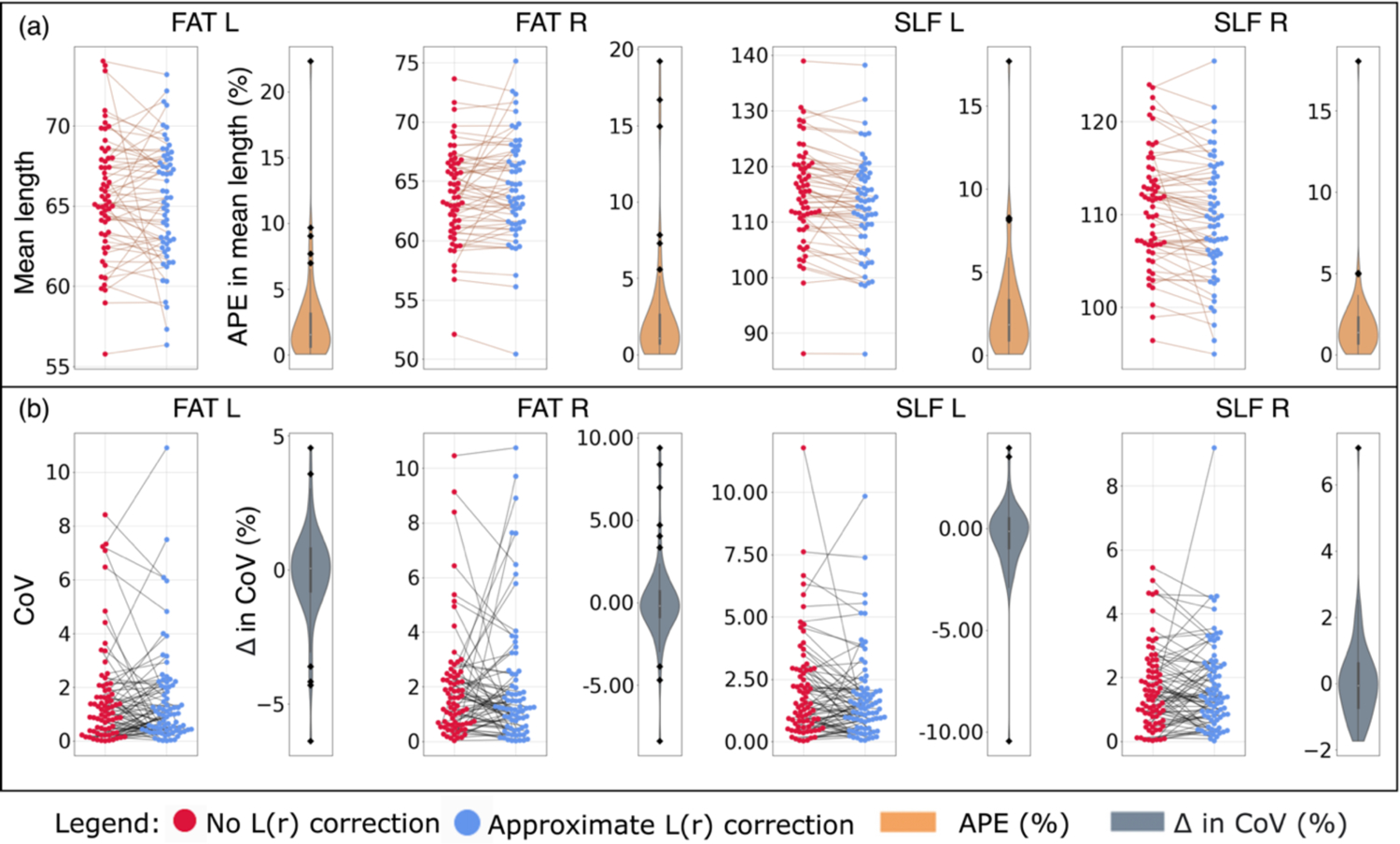
Effects of L(r) correction on (a) the mean length and (b) the within session variability in mean length for four bundles. (a) Each data point was the bundle’s computed mean length for a scan from a session in a subject with no correction (red dots) and approximate correction (blue dots). The data points from the same subjects are connected (brown lines) and the distribution of the APE in the data points connected was shown in brown. Notice, some subjects have a large effect (black dots). (b) Each data point was CoV of the bundle’s mean length for a within session observation with no correction (red dots) and approximate correction (blue dots). The data points from the same within session observations are connected (black lines) and the distribution of the difference in the data points connected was shown in grey. Again, some subjects have a large effect (black dots). The graphing tool range was limited within the range of the observed data. Abbreviations: CoV, coefficient of variation, APE, absolute percent error, FAT, frontal aslant tract [L/R], and SLF, superior longitudinal fasciculus [L/R])

Figure 6 shows the same effects before and after L(r) correction as Figure 5, but for bundle volume. For the impact on bundle-wise mean volume directly (Figure 6a), we find that the median APE was 13.603% for FAT L, 11.640% for FAT R, 5.510% for SLF L, and 5.910% for SLF_R. For within session variability in bundle-volume (Figure 6b), we observe the median difference in CoV before and after L(r) correction was −3.10% for FAT L, −1.02% for FAT R, −0.61% for SLF L, and −0.33% in SLF R. Again, negative difference means correction decreased the variability in computed measure and vise-versa. Similar to Figure 3, we observe a subset of subjects with a large negative impact and positive impact after L(r) correction in the bundles’ computed measures (Figure 5, 6 back dots). This suggest same as Figure 3, subjects are impacted differently, some exhibit large changes (Figure 5, 6 back dots) while most others exhibit a smaller change. Since, there are more subjects with a smaller impact, we observe the median is close 0 at population level.

Figure 6.

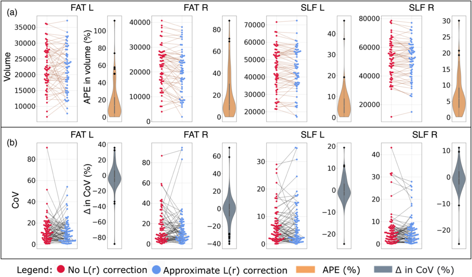
Effects of L(r) correction on (a) the volume and (b) the within session variability in volume of four bundles. (a) Each data point was the bundle’s computed volume for a scan from a session in a subject with no correction (red dots) and approximate correction (blue dots). The data points from the same subjects are connected (brown lines) and the distribution of the APE in the data points connected was shown in brown. Notice, some subjects have a large effect (black dots). (b) Each data point was CoV of the bundle’s volume for a within session observation with no correction (red dots) and approximate correction (blue dots). The data points from the same within session observations are connected (black lines) and the distribution of the difference in the data points connected was shown in grey. Again, some subjects have a large effect (black dots). The graphing tool range was limited within the range of the observed data. Abbreviations: CoV, coefficient of variation, APE, absolute percent error, FAT, frontal aslant tract [L/R], and SLF, superior longitudinal fasciculus [L/R])

To understand the regional impacts of L(r) correction, we visualize the APE in bundles across 61 subjects (Figure 7). The region with the highest impact after L(r) correction for FA was 2.089% in SLF R, MD was 5.338% in the corpus callosum pre/post central gyri (CCPrPo), AD was 5.084% in CCPrPo, RD was 5.466% in CCPrPo, and V1 was 1.7° in FAT R. This indicate that highest impacts due to L(r) correction mainly occur in frontal lobe.

Figure 7.

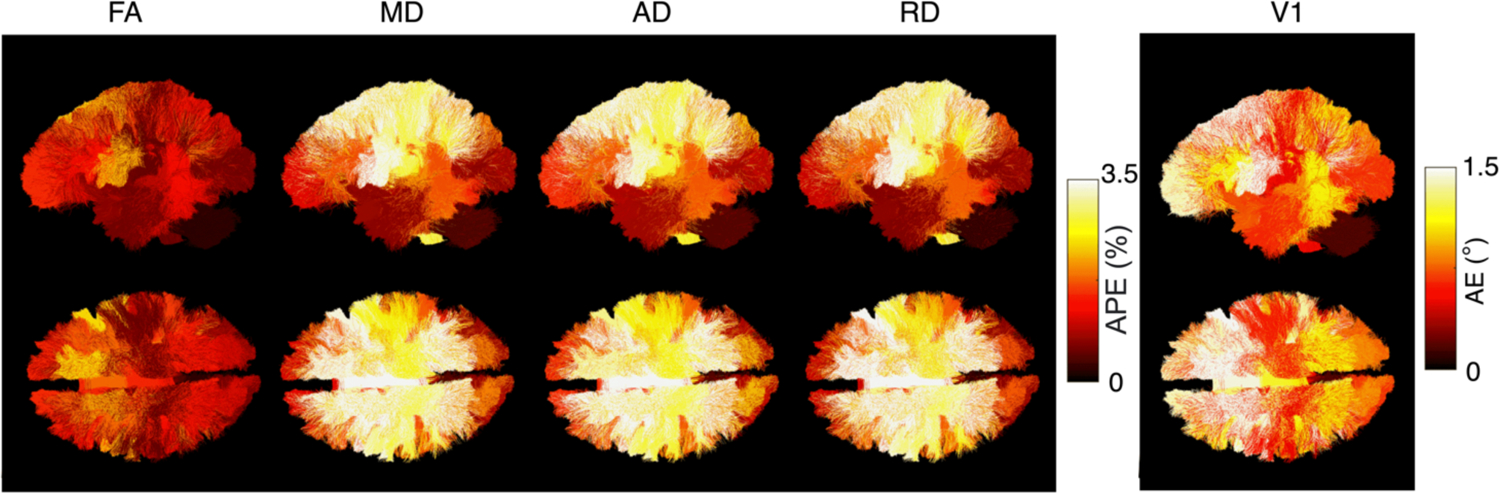
Sagittal and axial views of regional effects of nonlinear fields on bundles across 61 subjects. Anterior parts of the brain are impacted the most. V1 was impacted up to 1.5°.

DISCUSSION

Gradient nonlinearities may bias tractography results, which are an integral part of neuroscientific advances in biological modeling and biomarkers for neurological diseases. In this work, we characterized the impact of nonlinear gradient field correction on connectomes and bundle segmentation. Understanding the changes after correction of L(r) fields is essential when including such steps in practice in preprocessing pipelines.

From the results, we interpret three conclusions. First, the changes in the computed measures could be due to the reproducibility of these measure and independent of the L(r) correction. We notice after L(r) correction as CoV range increases, the median APE increases. For instance, the within session variability for global efficiency is up to 20% CoV and the median of APE after L(r) correction is 3.4%. Studies have shown that sensitivity of reconstruction of the bundles across subjects is between 76 and 94% and thus, suggesting the APE in volume and mean length could be due to reproducibility of computed measure as a consequence of the probabilistic nature of tractography [30, 32]. Second, approximate L(r) correction does not affect population level analysis due to the theoretical lack of change of orientation. However, we observe considerable subject-specific positive and negative impacts of L(r) correction for both the computed measure directly and the variability of computed measures. While we cannot clearly elucidate the underlying reason, we suspect this change could be due to factors such as SNR, motion, head size, and position of the subject in the scanner [9]. Third, the region with the highest impact was the frontal lobe, as confirmed in previous research [9].

This study provides a framework to interpret characteristics of approximate L(r) correction, how it alters and impacts the precision and accuracy of diffusion scalar measures, graph theory measures, and bundle segmentation measures. This study is limited to one correction technique. Thus, the next step would be to compare these findings with empirical Bammar voxel-wise gradient table correction [10]. Clearly, further research is required to understand how the interaction of other distortions such as noise with gradient nonlinear affect tractography as well as individual nodes and edges. Finally, we intend to use the insight from these studies to determine the consequence of L(r) correction in diffusion preprocessing pipelines.

REFERENCES

- [1].Nucifora PG, Verma R, Lee S-K, and Melhem ER, “Diffusion-tensor MR imaging and tractography: exploring brain microstructure and connectivity,” RADIOLOGY-OAK BROOK IL-, vol. 245, no. 2, p. 367, 2007. [DOI] [PubMed] [Google Scholar]
- [2].Assaf Y and Pasternak O, “Diffusion tensor imaging (DTI)-based white matter mapping in brain research: a review,” Journal of molecular neuroscience, vol. 34, no. 1, pp. 51–61, 2008. [DOI] [PubMed] [Google Scholar]
- [3].Ciccarelli O, Catani M, Johansen-Berg H, Clark C, and Thompson A, “Diffusion-based tractography in neurological disorders: concepts, applications, and future developments,” The Lancet Neurology, vol. 7, no. 8, pp. 715–727, 2008. [DOI] [PubMed] [Google Scholar]
- [4].Essayed WI, Zhang F, Unadkat P, Cosgrove GR, Golby AJ, and O’Donnell LJ, “White matter tractography for neurosurgical planning: A topography-based review of the current state of the art,” NeuroImage: Clinical, vol. 15, pp. 659–672, 2017. [DOI] [PMC free article] [PubMed] [Google Scholar]
- [5].Shi F, Yap P-T, Gao W, Lin W, Gilmore JH, and Shen D, “Altered structural connectivity in neonates at genetic risk for schizophrenia: a combined study using morphological and white matter networks,” Neuroimage, vol. 62, no. 3, pp. 1622–1633, 2012. [DOI] [PMC free article] [PubMed] [Google Scholar]
- [6].Sumanaweera TS, Adler JR Jr, Napel S, and Glover GH, “Characterization of spatial distortion in magnetic resonance imaging and its implications for stereotactic surgery,” Neurosurgery, vol. 35, no. 4, pp. 696–704, 1994. [DOI] [PubMed] [Google Scholar]
- [7].Hurd R, Deese A, Johnson MN, Sukumar S, and Van Zijl P, “Impact of differential linearity in gradient-enhanced NMR,” Journal of Magnetic Resonance, Series A, vol. 2, no. 119, pp. 285–288, 1996. [Google Scholar]
- [8].Mesri HY, David S, Viergever MA, and Leemans A, “The adverse effect of gradient nonlinearities on diffusion MRI: From voxels to group studies,” NeuroImage, vol. 205, p. 116127, 2020. [DOI] [PubMed] [Google Scholar]
- [9].Guo F et al. , “The effect of gradient nonlinearities on fiber orientation estimates from spherical deconvolution of diffusion magnetic resonance imaging data,” Human Brain Mapping, vol. 42, no. 2, pp. 367–383, 2021. [DOI] [PMC free article] [PubMed] [Google Scholar]
- [10].Bammer R et al. , “Analysis and generalized correction of the effect of spatial gradient field distortions in diffusion-weighted imaging,” Magnetic Resonance in Medicine: An Official Journal of the International Society for Magnetic Resonance in Medicine, vol. 50, no. 3, pp. 560–569, 2003. [DOI] [PubMed] [Google Scholar]
- [11].Malyarenko DI, Ross BD, and Chenevert TL, “Analysis and correction of gradient nonlinearity bias in apparent diffusion coefficient measurements,” Magnetic resonance in medicine, vol. 71, no. 3, pp. 1312–1323, 2014. [DOI] [PMC free article] [PubMed] [Google Scholar]
- [12].Rogers BP et al. , “Phantom-based field maps for gradient nonlinearity correction in diffusion imaging,” in Medical Imaging 2018: Physics of Medical Imaging, 2018, vol. 10573: International Society for Optics and Photonics, p. 105733N. [DOI] [PMC free article] [PubMed] [Google Scholar]
- [13].Rogers BP, Blaber J, Welch EB, Ding Z, Anderson AW, and Landman BA, “Stability of gradient field corrections for quantitative diffusion MRI,” in Medical Imaging 2017: Physics of Medical Imaging, 2017, vol. 10132: International Society for Optics and Photonics, p. 101324X. [DOI] [PMC free article] [PubMed] [Google Scholar]
- [14].Hansen CB et al. , “Empirical field mapping for gradient nonlinearity correction of multi-site diffusion weighted MRI,” Magnetic Resonance Imaging, vol. 76, pp. 69–78, 2021. [DOI] [PMC free article] [PubMed] [Google Scholar]
- [15].Markl M et al. , “Generalized reconstruction of phase contrast MRI: analysis and correction of the effect of gradient field distortions,” Magnetic Resonance in Medicine: An Official Journal of the International Society for Magnetic Resonance in Medicine, vol. 50, no. 4, pp. 791–801, 2003. [DOI] [PubMed] [Google Scholar]
- [16].Newitt DC et al. , “Gradient nonlinearity correction to improve apparent diffusion coefficient accuracy and standardization in the american college of radiology imaging network 6698 breast cancer trial,” Journal of Magnetic Resonance Imaging, vol. 42, no. 4, pp. 908–919, 2015. [DOI] [PMC free article] [PubMed] [Google Scholar]
- [17].Tan ET, Marinelli L, Slavens ZW, King KF, and Hardy CJ, “Improved correction for gradient nonlinearity effects in diffusion-weighted imaging,” Journal of Magnetic Resonance Imaging, vol. 38, no. 2, pp. 448–453, 2013. [DOI] [PubMed] [Google Scholar]
- [18].Rudrapatna U, Parker GD, Roberts J, and Jones DK, “A comparative study of gradient nonlinearity correction strategies for processing diffusion data obtained with ultra-strong gradient MRI scanners,” Magnetic Resonance in Medicine, vol. 85, no. 2, pp. 1104–1113, 2021. [DOI] [PMC free article] [PubMed] [Google Scholar]
- [19].Kanakaraj P et al. , “Mapping the impact of non-linear gradient fields on diffusion MRI tensor estimation,” in Medical Imaging 2022: Image Processing, 2022, vol. 12032: SPIE, p. 1203203. [DOI] [PMC free article] [PubMed] [Google Scholar]
- [20].Yeh F. “Twitter thread.” https://twitter.com/FangChengYeh/status/1400621354546835463 (accessed Dec 03, 2021).
- [21].Sotiropoulos SN et al. , “Advances in diffusion MRI acquisition and processing in the Human Connectome Project,” Neuroimage, vol. 80, pp. 125–143, 2013. [DOI] [PMC free article] [PubMed] [Google Scholar]
- [22].Setsompop K et al. , “Pushing the limits of in vivo diffusion MRI for the Human Connectome Project,” Neuroimage, vol. 80, pp. 220–233, 2013. [DOI] [PMC free article] [PubMed] [Google Scholar]
- [23].Cai LY et al. , “MASiVar: Multisite, multiscanner, and multisubject acquisitions for studying variability in diffusion weighted MRI,” Magnetic resonance in medicine, vol. 86, no. 6, pp. 3304–3320, 2021. [DOI] [PMC free article] [PubMed] [Google Scholar]
- [24].Rheault F, “Analyse et reconstruction de faisceaux de la matière blanche,” Computer Science. Université de Sherbrooke, 2020. [Google Scholar]
- [25].Rogers BP, Blaber J, Welch EB, Ding Z, Anderson AW, and Landman BA, “Stability of gradient field corrections for quantitative diffusion MRI,” in Medical Imaging 2017: Physics of Medical Imaging, 2017, vol. 10132: SPIE, pp. 1272–1278. [DOI] [PMC free article] [PubMed] [Google Scholar]
- [26].Cai LY et al. , “PreQual: An automated pipeline for integrated preprocessing and quality assurance of diffusion weighted MRI images,” Magnetic resonance in medicine, vol. 86, no. 1, pp. 456–470, 2021. [DOI] [PMC free article] [PubMed] [Google Scholar]
- [27].Theaud G, Houde J-C, Boré A, Rheault F, Morency F, and Descoteaux M, “TractoFlow: A robust, efficient and reproducible diffusion MRI pipeline leveraging Nextflow & Singularity,” NeuroImage, vol. 218, p. 116889, 2020. [DOI] [PubMed] [Google Scholar]
- [28].Rheault F et al. , “Connectoflow: A cutting-edge Nextflow pipeline for structural connectomics,” in International Society for Magnetic Resonance in Medicine Annual Meeting & Exhibition, 2021. [Google Scholar]
- [29].Huo Y et al. , “3D whole brain segmentation using spatially localized atlas network tiles,” NeuroImage, vol. 194, pp. 105–119, 2019. [DOI] [PMC free article] [PubMed] [Google Scholar]
- [30].Garyfallidis E et al. , “Recognition of white matter bundles using local and global streamline-based registration and clustering,” NeuroImage, vol. 170, pp. 283–295, 2018. [DOI] [PubMed] [Google Scholar]
- [31].Rubinov M and Sporns O, “Complex network measures of brain connectivity: uses and interpretations,” Neuroimage, vol. 52, no. 3, pp. 1059–1069, 2010. [DOI] [PubMed] [Google Scholar]
- [32].Cousineau M et al. , “A test-retest study on Parkinson’s PPMI dataset yields statistically significant white matter fascicles,” NeuroImage: Clinical, vol. 16, pp. 222–233, 2017. [DOI] [PMC free article] [PubMed] [Google Scholar]
- [33].Farrell JA et al. , “Effects of SNR on the accuracy and reproducibility of DTI-derived fractional anisotropy, mean diffusivity, and principal eigenvector measurements at 1.5 T,” Journal of magnetic resonance imaging: JMRI, vol. 26, no. 3, p. 756, 2007. [DOI] [PMC free article] [PubMed] [Google Scholar]
- [34].Landman BA, Farrell JA, Jones CK, Smith SA, Prince JL, and Mori S, “Effects of diffusion weighting schemes on the reproducibility of DTI-derived fractional anisotropy, mean diffusivity, and principal eigenvector measurements at 1.5 T,” Neuroimage, vol. 36, no. 4, pp. 1123–1138, 2007. [DOI] [PubMed] [Google Scholar]