Research on the performance degradation assessment method of a mine hoist braking system based on variable step-size fruit fly optimization algorithm–complex Gaussian wavelet support vector data description

Abstract

According to the characteristics of the constant deceleration braking system of hoist, a variable step-size fruit fly optimization algorithm–complex Gaussian wavelet support vector data description method is proposed in this article to evaluate the performance of the brake system. This method takes the pressure–time curve of safety braking as the characteristic data and extracts the candidate characteristic parameters from it. After the comprehensive evaluation of the characteristic parameters based on correlation, monotonicity, and predictability, the characteristic parameters are selected to evaluate the overall performance of the brake system. The proposed variable step-size fruit fly optimization algorithm–complex Gaussian wavelet support vector data description model avoids the situation where the classical Drosophila optimization algorithm is easy to fall into the local optimum. The reliability of the proposed method is verified by the simulation data, and the practicability of the proposed method is verified by the test-bed data. The performance evaluation model of variable step-size fruit fly optimization algorithm–complex Gaussian wavelet support vector data description is constructed, which realizes the quantitative evaluation of the brake system health state and provides technical support for the condition-based maintenance and intelligent maintenance of the hoist brake system.

Introduction

As the key equipment in the mine production, the mine hoist connects the ground and the underground and shoulders the important task of lifting coal, ore, personnel, materials, and equipment. With the rapid development of science and technology, the mine hoist is becoming larger scale, more complicated, more automated and more intelligent. The braking system of the hoist is the last barrier to ensure the safe operation of the hoist. In the process of operation, due to burn-in, wear, and other reasons, its performance will gradually degrade, which not only reduces the reliability of the braking system, but also increases the possibility of hoist failure. Once the braking system fails, it may affect the hoist or even force shut down the whole mine, causing huge property losses and casualties, even a catastrophic accident. Therefore, it is imperative to improve the safety and reliability of the hoist braking system. The research on performance degradation assessment of the braking system can help us to know the degree and trend of performance degradation, which can effectively avoid sudden failure of equipment and reduce production loss and equipment maintenance cost.

As one of the core technologies of intelligent maintenance, equipment performance degradation assessment has been widely studied in recent years. Liu et al. ¹ achieved high long-term prediction accuracy by comparing signatures from any two degradation processes using measures of similarity that form a match matrix. Dang and Jiang ² realized prediction of degradation of electronic products by combining correlation analysis and the back propagation (BP) wavelet neural network. Wang et al. ³ used Locally Linear Embedding (LLE) popular learning and the fuzzy C-means method to assess the performance degradation of bearings. Zhang et al. ⁴ used the Principal Component Analysis-Cerebellar Model Articulation Controller (PCA-CMAC) method to assess the condition of drill bits. The algorithm proposed by Jia et al. ⁵ assesses the health condition of wind turbines by performing principal component analysis (PCA) on the quasi-linear region of the power curve. Wang et al. ⁶ established a performance degradation model of wind turbine bearings based on the Wiener process, and the maximum likelihood method is used to assess the performance and residual life of bearings. Wang et al. ⁷ assessed bearing performance and predicted the residual life through a proportional hazard model. Shouqiang et al. ⁸ proposed a quantitative assessment method of the rolling bearing health condition based on chaotic fruit fly optimization algorithm–multi kernel hypersphere support vector machine (CFOA–MKHSVM), and the effectiveness and practicability of the proposed method are verified by experiments. Shuo et al., ⁹ aiming to solve the problem of insensitivity of the support vector data description (SVDD) algorithm to early fault of rolling bearings and difficulty in parameter selection, proposed a performance degradation assessment method of rolling bearings based on fruit fly optimization algorithm–wavelet support vector data description (FOA–WSVDD). Zhen ¹⁰ proposed a performance degradation assessment method of reciprocating compressors based on the SVDD algorithm. Wang et al. ¹¹ and Xi et al. ¹² used the linear regression method to transform the measured values of several performance parameters of turbofan engines and obtained the performance degradation condition index values. Yan et al. ¹³ assessed the performance degradation of elevator doors by using the logistic regression method. Wenzhu, ¹⁴ based on the condition data of the equipment operation process, proposed a method of equipment performance degradation assessment based on statistical pattern recognition and introduced health indexes to quantify the performance condition of current equipment. Finally, the effectiveness and practicability of the proposed method are proved by taking drilling equipment as the research object. Applying the evidence reasoning theory, Yaogang ¹⁵ proposed a health condition assessment method of wind turbines based on the multi-class evidence method. Hongbo ¹⁶ realized health condition assessment of the tractive power supply system by using a fuzzy comprehensive assessment. Luoping ¹⁷ presented a performance degradation assessment model of hydroelectric unit vibration parameters based on least square–support vector machine (LS–SVM). Jian ¹⁸ proposed a performance assessment method of hydroelectric units based on the transient start-up process and improved the dynamic normalization algorithm. This method can detect abnormal units as early as possible and reduce the probability of accidents. Bin ¹⁹ presented a performance degradation modeling approach based on functional principal component analysis (FPCA) with normalized running time. The modeling approach based on FPCA is validated by performance degradation data of aeroengine and DC cooling fan. Xiaolong ²⁰ presented a tree representation method of aeroengine-monitoring data, defined the distance of the monitoring data tree, and used this distance to access aeroengine performance degradation.

The Swarm intelligence optimization algorithm has the advantages of global optimal solution, low computational complexity, and good robustness, and it has become a research hotspot in the world.^21,22 The research fields mainly include the krill herd algorithm,^23–25 parallel hurricane optimization algorithm, ²⁶ oriented cuckoo search algorithm, ²⁷ Hybridizing harmony search algorithm, ²⁸ Monarch butterfly optimization, ²⁹ Binary moth search algorithm,^30,31 Earthworm optimization algorithm, ⁶ and so on. Nowadays, these Swarm intelligence computing methods have been widely used in path planning, image processing, data mining, intelligent control, network optimization, and other fields.

According to the features of the mine hoist braking system and the pressure–time curve of the braking system during safe braking, this article presents an assessment method of braking performance of the braking system based on variable step-size fruit fly optimization algorithm–complex Gaussian wavelet support vector data description (VSFOA–CGWSVDD).

The layout of the article is as follows. The VSFOA–CGWSVDD performance evaluation model is described in Section “Performance Evaluation Model of VSFOA–CGWSVDD.” Extraction and selection methods of feature parameters are described in Section “Extraction and Selection of Feature Parameters.” The algorithms are introduced in Section “Performance Degradation Model Based on VSFOA–CGWSVDD” with a particular focus on the SVDD method, complex Gaussian wavelet function, VSFOA, and the method and step of constructing the VSFOA–CGWSVDD performance assessment model. The reliability of the VSFOA–CGWSVDD performance assessment model is verified in Section “Simulation Experiment” by simulations. The practicability of the VSFOA–CGWSVDD performance assessment model is verified in Section “Test Verification.” The advantages and disadvantages of the method are summarized in Section “Conclusion.”

Performance evaluation model of VSFOA–CGWSVDD

In the VSFOA–CGWSVDD performance assessment model, first, the feature data are extracted from the pressure–time curve of brake during safety braking. Then, the feature vectors of performance degradation assessment are selected according to the comprehensive assessment rules. Next, the VSFOA–CGWSVDD hypersphere model is constructed by using these feature vectors and is used as a measurement standard for on-line monitoring of the health condition of the braking system. Finally, the pressure–time data collected from the braking system test can be brought into the VSFOA–CGWSVDD model after pretreatment, feature extraction, and selection, and the performance degradation index can be obtained. The used computer is PC-compatible desktop that uses the Intel Core i3 processor with 4GB Memory and 64-bit operation system. The MATLAB software version 2017a was used for the simulation experiments. The flow chart is shown in Figure 1.

Figure 1.

The flow chart of the performance assessment system.

Extraction and selection of feature parameters

Calculation of alternative feature parameter sets

Time-domain and frequency-domain features based on statistical theory are widely used in fault diagnosis and performance degradation assessment because of their clear physical meaning, simple calculation, and strong practicability.

In this article, 29 kinds of feature indexes are selected to form the alternative feature set of performance degradation assessment, and then the feature vectors with high sensitivity to performance degradation are selected to evaluate the performance degradation through feature assessment.

The 29 feature indices are dimensional time-domain indices, dimensionless time-domain indices, eight normalized subband energy of the third layer of three-layer wavelet packet decomposition and reconstruction ( $E_{3,0},E_{3,1},E_{3,2},E_{3,3},E_{3,4},E_{3,5},E_{3,6},E_{3,7}$ ), and six different percentiles. Dimensional time-domain indices include mean $\overline{x}$ , root mean square ${\overline{x}}_x$ , geometric mean $x_g$ , harmonic mean $H_n$ , range $r$ , and central moment features of order 2 to 7 $M_2^{\prime },M_3^{\prime },M_4^{\prime },M_5^{\prime },M_6^{\prime },M_7^{\prime }$ . Dimensionless time-domain indexes include waveform index $S_f$ , peak index $C_f$ , kurtosis index $K_f$ , and margin index $C{L}_f$ . Six different percentiles consist of $P_{98},P_{95},P_{92},P_{90},P_{80},P_{50}$ . Let $X$ represent an n-dimensional sample vector: $X=[x_1,x_2,\cdots ,x_n]$ . $p_i$ is defined as the value of the first i% of the n data of vector X arranged in small to large order. The other alternative feature set indicators and their definitions are shown in Table 1.

Table 1.

Alternative Feature Indicators and Their Parameter Definitions.

Feature indicator	Parameter definition	Feature indicator	Parameter definition
Mean	$\overline{x}=\frac{1}{n}\sum _{i=1}^n{x}_i$	Root mean square	${\overline{x}}_x=\sqrt{\frac{1}{n}\sum _{i=1}^n{x}_i^2}$
Geometric mean	$x_g=\sqrt[n]{x_1·x_2\cdots x_n}$	Range	$r=x_{\max }-x_{\min }$
Harmonic mean	$H_n=\frac{n}{\sum _{i=1}^n\frac{1}{x_i}}$	Waveform index	$S_f=\frac{\sqrt{\frac{1}{n}\sum _{i=1}^n{x}_i^2}}{\left|\overline{x}\right|}$
Peak index	$C_f=\frac{x_{\max }}{\sqrt{\frac{1}{n}\sum _{i=1}^n{x}_i^2}}$	$E_{3,0}$	$E_{3,0}={\int }_0^{t_1}{\left|x_{3,0}^k\left(t\right)\right|}^2\mathrm{dt}=\sum _{k=1}^m{\left|x_{3,0}^k\right|}^2$
Kurtosis index	$K_f=\frac{\frac{1}{n}{\sum _{i=1}^n(x_i-\overline{x})}^4}{{\left[\frac{1}{n}{\sum _{i=1}^n(x_i-\overline{x})}^2\right]}^2}$	$E_{3,1}$	$E_{3,0}={\int }_0^{t_1}{\left|x_{3,0}^k\left(t\right)\right|}^2\mathrm{dt}=\sum _{k=1}^m{\left|x_{3,0}^k\right|}^2$
Margin index	$C{L}_f=\frac{x_{\max }}{{\left(\frac{1}{n}\sum _{i=1}^n\sqrt{|x_i-\overline{x}|}\right)}^2}$	$E_{3,2}$	$E_{3,2}={\int }_{t_1}^{t_2}{\left|x_{3,2}^k\left(t\right)\right|}^2\mathrm{dt}=\sum _{k=1}^m{\left|x_{3,2}^k\right|}^2$
2-Order moment (variance)	$M_2^{\prime }=\frac{1}{n}\sum _{i=1}^n{(x_i-\overline{x})}^2$	$E_{3,3}$	$E_{3,3}={\int }_{t_2}^{t_3}{\left|x_{3,3}^k\left(t\right)\right|}^2\mathrm{dt}=\sum _{k=1}^m{\left|x_{3,3}^k\right|}^2$
3-Order moment (skewness)	$M_3^{\prime }=\frac{1}{n}\sum _{i=1}^n{(x_i-\overline{x})}^3$	$E_{3,4}$	$E_{3,4}={\int }_{t_3}^{t_4}{\left|x_{3,4}^k\left(t\right)\right|}^2\mathrm{dt}=\sum _{k=1}^m{\left|x_{3,4}^k\right|}^2$
4-Order moment	$M_4^{\prime }=\frac{1}{n}\sum _{i=1}^n{(x_i-\overline{x})}^4$	$E_{3,5}$	$E_{3,5}={\int }_{t_4}^{t_5}{\left|x_{3,5}^k\left(t\right)\right|}^2\mathrm{dt}=\sum _{k=1}^m{\left|x_{3,5}^k\right|}^2$
5-Order moment	$M_5^{\prime }=\frac{1}{n}\sum _{i=1}^n{(x_i-\overline{x})}^5$	$E_{3,6}$	$E_{3,6}={\int }_{t_5}^{t_6}{\left|x_{3,6}^k\left(t\right)\right|}^2\mathrm{dt}=\sum _{k=1}^m{\left|x_{3,6}^k\right|}^2$
6-Order moment	$M_6^{\prime }=\frac{1}{n}\sum _{i=1}^n{(x_i-\overline{x})}^6$	$E_{3,7}$	$E_{3,7}={\int }_{t_6}^{t_7}{\left|x_{3,7}^k\left(t\right)\right|}^2\mathrm{dt}=\sum _{k=1}^m{\left|x_{3,7}^k\right|}^2$
7-Order moment	$M_7^{\prime }=\frac{1}{n}\sum _{i=1}^n{(x_i-\overline{x})}^7$

Assessment index of feature parameters

• (1) Correlation

$$\mathrm{Corr}(x)=\frac{|n\sum _{i=1}^n{x}_i{t}_i-\sum _{i=1}^n{x}_i\sum _{i=1}^n{t}_i|}{\sqrt{\left[n{\sum _{i=1}^n{x_i}^2-\left[\sum _{i=1}^n{x}_i\right]}^2\right][n\sum _{i=1}^n{t_i}^2-{\left[\sum _{i=1}^n{t}_i\right]}^2]}}$$ (1)

where $X=[x_1,x_2,\cdots ,x_n]$ is the performance degradation sequence. n is the number of monitoring in the whole process of performance degradation. $T=[t_1,t_2,\cdots ,t_n]$ is the sampling time sequences of performance degradation sequences.

• (2) Monotonicity

$$\mathrm{Mon}(x)=\frac{|\sum _{i=1}^n\delta (x_i-x_{i-1})-\sum _{i=1}^n\delta (x_{i-1}-x_i)|}{n-1}$$ (2)

where $X=[x_1,x_2,\cdots ,x_n]$ is the performance degradation sequence. $\delta \left(x\right)=\{\begin{array}{c}\begin{array}{cc}1\hfill & x⩾0\hfill \end{array}\hfill \\ \multicolumn{1}{c}{\begin{array}{cc}0\hfill & x<0\hfill \end{array}}\end{array}$ is the unit step function.

• (3) Predictive index

$$\mathrm{Pre}(x)=\exp (-\frac{\sigma \left(x_f\right)}{|x_1-x_n|})$$ (3)

where $x_1$ is the value of feature parameters at the initial time. $x_n$ is the value of feature parameters at the failure time. $\sigma \left(x_f\right)$ is the standard deviation of feature parameters.

Comprehensive assessment method of feature parameters

In order to consider the contribution rate of multiple assessment indexes synthetically, the scores of each assessment index should be normalized first. That is, the scores of each assessment index should be mapped to the range of [0,1], and the normalized processing formula is as follows

$$x_{\mathrm{ij}}^{\prime }=\frac{x_{\mathrm{ij}}-x_{\min }^j}{x_{\max }^j-x_{\min }^j}$$ (4)

where $x_{\mathrm{ij}}$ and $x_{\mathrm{ij}}^{\prime }$ are the values before and after normalization of the ith feature of the jth assessment index, and $x_{\max }^j$ and $x_{\min }^j$ are the maximum and minimum scores of the jth assessment index, respectively.

Second, the weights of each assessment index are determined by expert decision, and the weight vector of the assessment index determined in this article is $(w_{1,}{w}_2,w_3)=(0.3,0.3,0.4)$ . That is, the correlation and monotonicity indexes are given smaller weights, and the predictive indexes are given larger weights.

Defining the score of each feature value is

$$Q_m=\sum _{i=1}^3{t}_i^m{w}_i\begin{array}{c}m=1,2,\cdots ,29\hfill \end{array}$$ (5)

where $t_i^m$ denotes the score of the ith assessment index of the mth feature value, i=1,2,3, which denotes correlation, monotonicity, and predictability, respectively. $w_i$ denotes the corresponding weight of each assessment index.

Then, the mth feature value is judged to be optimal by the criterion of feature selection. The criterion of feature selection is as follows

$$\{\begin{array}{c}\begin{array}{c}{Q}_m⩾Q_H\hfill \end{array}\begin{array}{cc}\Rightarrow \hfill & \mathrm{Preferred}\mathrm{feature}\mathrm{value}\hfill \end{array}\hfill \\ \multicolumn{1}{c}{\begin{array}{c}{Q}_m<Q_H\hfill \end{array}\begin{array}{cc}\Rightarrow \hfill & \mathrm{Un}-\mathrm{preferred}\mathrm{feature}\mathrm{value}\hfill \end{array}}\end{array}$$ (6)

where $Q_H$ is the threshold of feature value selection.

Performance degradation model based on VSFOA–CGWSVDD

SVDD

SVDD was proposed by Tax in 1999. ³² SVDD has been widely used in anomaly detection and classification in recent years. The core idea of SVDD is to construct a minimal volume enclosed hypersphere in high-dimensional space, which can contain the data set of the described object. The data description boundary of the hypersphere is obtained. Samples inside the hypersphere boundary are defined as target classes, and samples outside the hypersphere boundary are defined as non-target classes.

For a given sample of the same class, there is a data set ${\left(x_i\right)}_i^N$ containing N objects in any n-dimensional space $R^n$ , and a minimal volume hypersphere can be found that include all data $x_i$ . The minimum hypersphere is defined as $F(R,a)$

$$\{\begin{array}{c}F(R,a,\xi )=R^2+C\sum _{i=1}^N{\xi }_i\hfill \\ \multicolumn{1}{c}{{\begin{array}{cc}s.t.\hfill & {\Vert \phi \left(x_i\right)-a\Vert }^2\le R^2+\xi \hfill \end{array}}_i\begin{array}{cc},\hfill & {\xi }_i⩾0\begin{array}{cc},\hfill & i=1,2,\cdots ,n\hfill \end{array}\hfill \end{array}}\end{array}$$ (7)

where R is the radius of the hypersphere. a is the position of the center of the hypersphere. ${\xi }_i$ is the slack variable, ${\xi }_i⩾0$ . $C$ is the penalty coefficient, C > 0.

For the convex quadratic programming problem mentioned above, the Lagrange optimization method can be used to transform them into their dual form

$$\{\begin{array}{c}L=\sum _{i=1}^N{\alpha }_i(x_i,x_i)-\sum _{i=1}^N\sum _{j=1}^N{\alpha }_i{\alpha }_j(x_i,x_j)\hfill \\ \multicolumn{1}{c}{\begin{array}{ccc}\begin{array}{cccc}s.t.\hfill & \sum _{i=1}^N{\alpha }_i=1\hfill & ,\hfill & 0\le {\alpha }_i\le C\hfill \end{array}\hfill & ,\hfill & i=1,2,\cdots ,N\hfill \end{array}}\end{array}$$ (8)

The minimum value of formula (8) is found and the optimal solution is recorded as ${\alpha }^{*}={({\alpha }_1^{*},{\alpha }_2^{*},\cdots ,{\alpha }_N^{*},)}^T$ .

Usually, the target data do not show spherical distribution, and it is linear inseparable in low-dimensional space. Therefore, the original data are mapped to high-dimensional feature space by using non-linear mapping, where the dual programming can be expressed as

$$\{\begin{array}{c}L=\sum _{i=1}^N{\alpha }_{i}K(x_i,x_i)-\sum _{i=1}^N\sum _{j=1}^N{\alpha }_i{\alpha }_{j}K(x_i,x_j)\hfill \\ \multicolumn{1}{c}{\begin{array}{ccc}\begin{array}{cccc}s.t.\hfill & \sum _{i=1}^N{\alpha }_i=1\hfill & ,\hfill & 0\le {\alpha }_i\le C\hfill \end{array}\hfill & ,\hfill & i=1,2,\cdots ,N\hfill \end{array}}\end{array}$$ (9)

where $K(x_i,x_j)=(\varphi \left(x_i\right),\varphi \left(x_j\right))$ .

The optimum solution ${\alpha }^{*}={({\alpha }_1^{*},{\alpha }_2^{*},\cdots ,{\alpha }_N^{*},)}^T$ can be obtained by finding the minimum value of formula (9). At this time, the formula for calculating the position of the spherical center of the minimum hypersphere in the feature space is as follows

$$a=\sum _{i=1}^N{\alpha }_i^{*}\varphi \left(x_i\right)$$ (10)

After mapping to the feature space, the corresponding sample point that is not zero in the optimal solution is the support vector of the hypersphere, recorded as B. The formula of the radius square of the minimum hypersphere is as follows

$$R^2=K(x_{\mathrm{sv}}·x_{\mathrm{sv}})-2\sum _{i=1}^N{\alpha }_{i}K(x_i,x_{\mathrm{sv}})+\sum _{i=1}^N\sum _{j=1}^N{\alpha }_i{\alpha }_{j}K(x_i,x_j)$$ (11)

The criteria for acceptance of test sample Z as the target sample are as follows

$$\Vert \varphi \left(z\right)-a{\Vert }^2=K(z·z)-2\sum _{i=1}^N{\alpha }_i^{*}(z,x_i)-\sum _{i=1}^N\sum _{j=1}^N{\alpha }_i^{*}{\alpha }_j^{*}K(x_i,x_j)\le R^2$$ (12)

The selection of the kernel function is a key problem in learning algorithms related to the kernel function. Because of the low computational complexity of the Gaussian kernel function, the fact that computation would not be restricted by the improvement of the dimension of feature space, and the extensive applicability to arbitrarily distributed samples, the Gaussian kernel function has been widely used. However, the Gauss kernel function cannot approximate any interface in the feature space, which greatly affects the accuracy and timeliness of the assessment. The kernel function based on the wavelet theory can effectively remedy this defect, so it can significantly improve the generalization ability of SVDD. ³³ In this article, the complex Gauss wavelet kernel function is used as the kernel function described by the support vector.

Complex gauss wavelet kernel function

Definition of the complex Gaussian wavelet kernel function

Definition 1: $\exists \psi \left(x\right)\ne 0,\psi \left(x\right)$ is a complex Gaussian wavelet

$$\psi \left(x\right)=C_p\exp (-\mathrm{ix})\exp (-x^2)$$

Definition 2: The complex Gaussian wavelet kernel function expression is as follows

$$\{\begin{array}{c}K(x,x^{\prime })=\underset{i=1}{\overset{n}{\Pi }}\psi \left(\frac{x_i-b_i}{a_i}\right)·\psi \left(\frac{x_i^{\prime }-b_i^{\prime }}{a_i^{\prime }}\right)\hfill \\ \multicolumn{1}{c}{s.t.\begin{array}{c}x,x^{\prime }\in R^n\hfill \end{array}}\\ \multicolumn{1}{c}{\begin{array}{cc}{a}_i,a_i^{\prime },b_i,b_i^{\prime }\in R;\hfill & \begin{array}{cc}{a}_i\ne 0,\hfill & a_i^{\prime }\ne 0\hfill \end{array}\hfill \end{array}}\end{array}$$ (13)

where $a_i$ and $a_i^{\prime }$ are expansion factors. $b_i$ and $b_i^{\prime }$ are displacement factors.

Proof of the complex Gaussian wavelet function satisfying the mercy condition

Proof:

Once $\phi \left(x\right)\in R$ and $\phi \left(x\right)\ne 0$ ,

We have

$$\begin{array}{c}\int {\int }_{R_n\times R_n}K(x,x^{\prime })\phi \left(x\right)\phi \left(x^{\prime }\right)\mathrm{dxd}{x}^{\prime }=\hfill \\ \int {\int }_{R_n\times R_n}\underset{i=1}{\overset{n}{\Pi }}[\psi \left(\frac{x_i-b_i}{a_i}\right)·\psi \left(\frac{x_i^{\prime }-b_i^{\prime }}{a_i^{\prime }}\right)]\phi \left(x\right)\phi \left(x^{\prime }\right)\mathrm{dxd}{x}^{\prime }=\hfill \\ \int {\int }_{R_n\times R_n}\underset{i=1}{\overset{n}{\Pi }}\{C_p\exp [-i\frac{x_i-b_i}{a_i}]\exp [-{\left(\frac{x_i-b_i}{a_i}\right)}^2]\times \hfill \\ C_p\exp [-i\frac{x_i^{\prime }-b_i^{\prime }}{a_i^{\prime }}]\exp [-{\left(\frac{x_i^{\prime }-b_i^{\prime }}{a_i^{\prime }}\right)}^2]\}\times \phi \left(x\right)\phi \left(x^{\prime }\right)\mathrm{dxd}{x}^{\prime }=\hfill \\ \{{\int }_{R^n}\underset{i=1}{\overset{n}{\Pi }}\{C_p\exp [-i\frac{x_i-b_i}{a_i}]\exp [-{\left(\frac{x_i-b_i}{a_i}\right)}^2]\times \phi \left(x\right)\mathrm{dx}\}\times \hfill \\ {\int }_{R^n}\underset{i=1}{\overset{n}{\Pi }}\{C_p\exp [-i\frac{x_i^{\prime }-b_i^{\prime }}{a_i^{\prime }}]\exp [-{\left(\frac{x_i^{\prime }-b_i^{\prime }}{a_i^{\prime }}\right)}^2]\times \phi \left(x^{\prime }\right)d{x}^{\prime }\}\}=\hfill \\ {\int }_{R^n}\underset{i=1}{\overset{n}{\Pi }}{\{C_p\exp [-i\frac{x_i-b_i}{a_i}]\exp [-{\left(\frac{x_i-b_i}{a_i}\right)}^2]\times \phi \left(x\right)\mathrm{dx}\}}^2>0\hfill \end{array}$$

Therefore, the complex Gaussian wavelet function satisfies the Mercy condition and can be used as the kernel function.

VSFOA

In 2011, Wen-Tsao Pan, inspired by fruit fly’s foraging behavior, proposed FOA. FOA is a new method to find global optimization based on the inference of fruit fly’s foraging behavior. Fruit fly is superior to other species in sensory perception, especially in olfaction and vision. Fruit fly can use the olfactory organs to collect the smell floating in the air. After flying near food according to the concentration of smell, they use sharp vision to find where food or peers gather and fly in that direction.

The FOA program is simple, easy to understand, and fast to converge, so it has been widely used. However, in classical FOA, the iteration step size of fruit fly in the foraging process is fixed and cannot be changed according to the actual problem, so there may be some problems in solving global optimization problems, such as low precision, slow convergence speed, and easy to fall into local optimization.^34–36 In order to overcome the shortcomings of classical FOA, the VSFOA is proposed in this article.

The idea of VSFOA is based on FOA. When fruit fly is looking for food initially, it searches in a wide range (global range). With the increase of iteration steps, the smell of food increases, and fruit fly gradually searches in a smaller range to improve the search accuracy and reduce the search time.

Because the small concentration is the reciprocal of the distance, the relationship between the step factor and search range is also reciprocal. The smaller the step factor, the larger the search range. Therefore, a small step factor should be selected at the beginning, and the step factor should be gradually increased. The definition of a step factor is as follows

$$\mathrm{Ste}{p}_i=\mathrm{Ste}{p}_{i-1}(1-\frac{\mathrm{ge}{n}_{i-1}}{\mathrm{ge}{n}_{\max }})$$ (14)

where $\mathrm{Ste}{p}_i$ is the iterative step size of the ith generation fruit fly. $\mathrm{ge}{n}_{i-1}$ is the (i–1)th evolution algebra of the first generation. $\mathrm{ge}{n}_{\max }$ is the maximum evolutionary algebra.

Establishment of the performance degradation assessment model

In order to establish the performance degradation evaluation model, it is necessary to first establish the CGWSVDD hypersphere model by using the performance reference samples of the braking system and then use the CGWSVDD model to classify the reference samples and the performance degradation samples. With the strong global search ability and high search accuracy of VSFOA, in the process of classification, the VSFOA–CGWSVDD model can be obtained by intelligent optimization of six parameters of $c_p,a_1,a_2,b_1,b_2$ in the CGWSVDD model and penalty factor C in SVDD at the same time. The detailed steps of the VSFOA–CGWSVDD model establishment are as follows:

• Step1: Parameter initialization. Initial population size, maximum iteration times, step factor, and initial position of fruit fly population

$$\begin{array}{c}\mathrm{Sizepop}=100;\hfill \\ \mathrm{ge}{n}_{\max }=100;\hfill \\ \mathrm{Step}=2/3;\hfill \\ \mathrm{length}=6;\hfill \\ x\_\mathrm{asis}=2*\mathrm{rand}(1,\mathrm{length})-1;\hfill \\ y\_\mathrm{asis}=2*\mathrm{rand}(1,\mathrm{length})-1;\hfill \end{array}$$

where $\mathrm{Step}$ is the step factor for fruit fly to search for food, and $\mathrm{Length}$ is the number of parameters to be optimized.

• Step2: Give fruit fly individual random directions and distances to search for food

$$\begin{array}{c}\mathrm{Position}\_x=x\_\mathrm{axis}+\mathrm{Step}*(2*\mathrm{rand}-1);\hfill \\ \mathrm{Position}\_y=y\_\mathrm{asis}+\mathrm{Step}*(2*\mathrm{rand}-1);\hfill \end{array}$$

• Step3: Because( the exact location) of the optimal solution is unknown, the distance $\mathrm{Dist}$ between the fruit fly individual and the origin is calculated first, and then the judgment value $\mathrm{Smell}$ of the odor concentration is calculated, which is the reciprocal of the distance

$$\begin{array}{c}\mathrm{Position}=[\mathrm{Position}\_x,\mathrm{Position}\_y];\hfill \\ \mathrm{Dist}=\sqrt{\mathrm{Position}\_x^2+\mathrm{Position}\_y^2};\hfill \\ \mathrm{Smell}=1/\mathrm{Direct};\hfill \end{array}$$

• Step4: The fitness value of a fruit fly individual was calculated by substituting $\mathrm{Smell}$ into the fitness function, that is, the judgment function of odor concentration. The CGWSVDD hypersphere model based on the brake system performance benchmark samples is established in this article and then is used for sample classification. Performance benchmark samples are defined as one class, corresponding category code is "1", and other performance degradation samples are the other class, corresponding category code is "–1". All samples are inputted into the CGWSVDD model, and the combination of the classification accuracy and the minimum number of support vectors (the minimum is defined as two support vectors) is defined as the fitness function of Drosophila individuals

$$\mathrm{Fitness}=((1-\frac{\mathrm{error}}{\mathrm{total}})+\frac{|\mathrm{erro}{r}_1-2|}{m})\times 100\%;$$

where $\mathrm{total}$ is the total number of samples to be classified, $\mathrm{Smell}$ is the number of samples classified incorrectly, $\mathrm{erro}{r}_1$ is the number of support vectors, and m is the total number of samples.

• Step5: Find out the fruit fly with the highest odor concentration in the fruit fly population

$$[\mathrm{Smell},\mathrm{Index}]=\max \left(\mathrm{Fitness}\right);$$

• Step6: Record the optimum concentration and the position coordinates of fruit fly

$$\begin{array}{c}\mathrm{best}\_\mathrm{Position}=\mathrm{Position}(\mathrm{Index},:);\hfill \\ \mathrm{best}\_\mathrm{Fitness}=\mathrm{Smell};\hfill \end{array}$$

• Step7: Enter iterative optimization. Step2–step5 is executed to determine whether the fitness function value is lower than the value of the previous iteration. If so, step6 is executed to update the optimal fitness value of the population and retain the optimal position, then step2–step5 is returned. If not, step 2–step 5 is directly returned to continue the iterative optimization until the end condition is reached.

• Step8: After the iteration, the best parameters $c_p,a_1,a_2,b_1,b_2\mathrm{and}C$ can be obtained, and the VSFOA–CGWSVDD model is established.

Definition of the performance index and assessment process of performance degradation

Definition of the performance index

The performance index of the equipment in this article is expressed by health degree (HD). HD indicates the degradation degree of the system performance with the range [0,1]; 1 indicates that the performance is the best, indicating that the equipment works in the optimal state, and 0 indicates that the performance is the worst, indicating that the equipment reaches the edge of the normal index and needs to strengthen monitoring and prepare for maintenance.

After the VSFOA–CGWSVDD hypersphere model is established, the data of all performance degradation stages are substituted into the VSFOA–CGWSVDD hypersphere model one by one, and the distance from each data point to the hypersphere center is calculated

$$D_{\mathrm{test}}=\sqrt{K(x_{\mathrm{test}},x_{\mathrm{test}})-2\sum _{i=1}^n{\alpha }_{i}K(x_{\mathrm{test}},x_i)+\sum _{i=1}^n\sum _{j=1}^n{\alpha }_i{\alpha }_{j}K(x_i,x_j)}$$ (15)

Taking D_test as the criterion of performance degradation assessment of brake system, the bigger it is, the farther the test sample deviates from the normal value, and the bigger the performance degradation degree of brake system is. In order to conform to human habitual thinking, the normalized distance of all performance degradation stages is defined as the performance degradation assessment index, that is, the HD of test samples is defined as

$$H{D}_{\mathrm{test}}=1-\frac{D_{\mathrm{test}}-D_{\min }}{D_{\max }-D_{\min }}$$ (16)

where $D_{\min }$ represents the minimum distance from the center of the VSFOA–CGWSVDD hypersphere model in all performance degradation stage samples, and $D_{\max }$ represents the maximum distance from the center of the VSFOA–CGWSVDD hypersphere model in all performance degradation stage samples.

Setting threshold of the self-adaptive performance degradation alarm

Large, complex, precise, and long-life equipment may not be able to obtain the whole life cycle data or can only obtain the data of the equipment operating in the optimal state. Therefore, it is necessary to set the performance degradation alarm threshold according to the 3σ-criterion. The 3σ-criterion is the simplest and most commonly used criterion for judging abnormal data, and its reliability is 99.73%. ³⁷ In the performance degradation assessment of the braking system, $\mu$ and σ are calculated by the performance index of sample data when the performance is healthy. $(\mu -3\sigma )$ is the threshold of the self-adaptive performance degradation alarm.

Flow chart of performance degradation assessment of the braking system

The flow chart of performance degradation assessment of the braking system is shown in Figure 2.

Figure 2.

Flow chart of performance degradation assessment based on VSFOA–CGWSVDD.VSFOA–CGWSVDD: variable step-size fruit fly optimization algorithm–complex Gaussian wavelet support vector data description.

Simulation experiment

Simulation of normal and performance degradation characteristic data

Using the simulation platform built by Juanjuan et al., ³⁸ the running speed of hoist is set to 10m/s, the deceleration is set to 3.5m/s ² , and the sampling frequency is set to 100Hz during safety braking. The sampling time starts with the braking signal from the control system and ends with the hoist speed dropping to zero. A total of 128 groups of pressure–time curves are simulated when the braking system properly operates and performance deteriorates, such as spring stiffness decreasing and friction coefficient decreasing. The first 30 groups are data samples under normal conditions, defined as the samples of the braking system in healthy conditions, and the rest are data samples of braking system performance degradation.

Feature extraction and selection

According to the method introduced in Section 2, 29 characteristic parameters of the pressure–time curve are extracted first. Second, the scores of correlation, monotonicity, and predictability are calculated according to formula (1)–(3), respectively. After that, normalizing these scores according to formula (4), the comprehensive assessment scores of each characteristic parameter are calculated according to formula (5). Finally, according to the comprehensive score of each feature parameter, the threshold of feature parameter selection is set to 0.55, and function (6) is used to determine whether each feature parameter is the optimal feature parameter. Fourteen characteristic parameters are selected, including percentile, mean, geometric mean, root mean square, waveform index, peak index, margin index, central moment characteristic, and the first normalized subband energy of the third layer of wavelet packet decomposition.

Establishment of the VSFOA–CGWSVDD model

VSFOA was used to optimize the parameters and penalty factor C in CGWSVDD. The comprehensive assessment of classification accuracy and minimum number of support vectors in the process of model training is taken as the fitness function of VSFOA. The initial step factor of individual fruit fly step is set to 1/1.5, population size is set to 100, and maximum iteration number is set to 100. After optimizing the CGWSVDD model by VSFOA, the parameters and penalty factor C of complex wavelet kernel function are obtained as shown in Table 2. All samples are substituted into the VSFOA–CGWSVDD model, and the classification accuracy of samples is 100%. The relationship between evolutionary generation and classification accuracy is shown in Figure 3.

Table 2.

Parameter Optimization Results in CGWSVDD.

Parameter	$c_p$	$a_1$	$a_2$	$b_1$	$b_2$	$C$
The best value	0.6	0.8	0.65	0.73	1.25	0.82

CGWSVDD: complex Gaussian wavelet support vector data description.

Figure 3.

The relationship between evolutional generation and classification accuracy of the VSFOA–CGWSVDD model.

VSFOA–CGWSVDD: variable step-size fruit fly optimization algorithm–complex Gaussian wavelet support vector data description.

As shown in Figure 3, the VSFOA–CGWSVDD model achieved 100% classification accuracy of all samples in the 55th iteration, which shows the practicability of the VSFOA–CGWSVDD method.

In order to verify the superiority of the VSFOA–CGWSVDD model, simulation samples are classified by using grid optimization algorithm–support vector data description (GOA–SVDD) model, FOA–SVDD model, FOA–CGWSVDD model, and VSFOA–CGWSVDD model. In order to make the optimization results more comparable, the population size of fruit fly is set to 100, the evolutional generation is set to 100, and the initial optimization step factor of VSFOA step is set to 2/3. The classification accuracy of GOV–SVDD is shown in Figure 4. The average classification accuracy and evolutional generation of other methods are shown in Figure 5.

Figure 4.

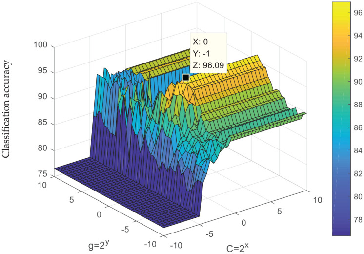
The classification accuracy of the GOA–SVDD model is shown in.

GOA–SVDD: grid optimization algorithmsupport vector data description.

Figure 5.

Evolutional generation and classification accuracy of various models.

As can be seen from Figures 4 and 5,

1. The optimal classification accuracy of GOA–SVDD is 96.09%, which is lower than other models.

2. In the SVDD models, the classification accuracy of the GOA–SVDD model is the lowest (96.09%), followed by FOA–SVDD (96.88%) and VSFOA–SVDD (98.44%).

3. In the CGWSVDD models, the VSFOA–CGWSVDD method achieves the optimal classification accuracy of 100% at the 55th iteration, and the FOA–CGWSVDD method achieves the classification accuracy of 99.2188%. VSFOA–CGWSVDD is better than FOA–CGWSVDD in the global search ability.

4. By comparing and analyzing the SVDD models with the CGWSVDD models, it can be seen that the classification accuracy of CGWSVDDs is better than that of SVDDs, regardless of the optimization method.

Through the above analysis, it can be concluded that the proposed VSFOA–CGWSVDD method can achieve the optimal classification accuracy of 100% at the 55th iteration. With the best classification accuracy, VSFOA can ensure that the optimization parameters are searched globally.

Performance degradation assessment based on VSFOA–CGWSVDD

After obtaining the VSFOA–CGWSVDD model, the characteristic vectors of all samples of the braking system are inputted into the VSFOA–CGWSVDD model one by one. The distance between the feature vectors and the center of the hypersphere model is calculated according to formula (15). The performance degradation assessment value of the test samples is obtained by normalizing the distance of all the calculated feature samples according to formula (16). With these assessment values as ordinates and sample numbers as abscissa, the performance degradation process curve of the braking system can be obtained, as shown in Figure 6. Using the same method, the performance degradation curve of the GOA–SVDD model can also be obtained, as shown in Figure 7.

Figure 6.

The performance degradation curve of the braking system based on the VSFOA–CGWSVDD model.

VSFOA–CGWSVDD: variable step-size fruit fly optimization algorithm–complex Gaussian wavelet support vector data description.

Figure 7.

The performance degradation curve of the braking system based on theGOA–SVDD model.

GOA–SVDD: grid optimization algorithm–support vector data description.

As can be seen from Figures 6 and 7,

1. The performance of the braking system shows a trend of gradual degradation. The performance degradation is slow in the early stage and fast in the later stage, which conforms to the law of equipment performance degradation. The performance degradation curves obtained by both methods can reflect the performance degradation of the equipment.

2. The fluctuation of the VSFOA–CGWSVDD model in the early stage of performance degradation is smaller than that of the GOA–SVDD model. The VSFOA–CGWSVDD model reaches the adaptive performance degradation threshold at the 31st simulation data, while the SVDD model reaches the threshold of adaptive alarm at the 39th simulation data. The VSFOA–CGWSVDD model monitors the performance degradation of the braking system earlier than the GOA–SVDD model.

Test verification

In order to verify the reliability and practicability of the proposed method, it is necessary to collect data on the test bench to verify the method. In order to reduce unnecessary damage to the test bench caused by safety braking, and also to make the research method transform smoothly into engineering, a fixed mode test scheme of safety braking performance is proposed in this article, which does not need loading in the implementation of the safety braking test. Load, speed, and braking deceleration of the hoist are all reduced appropriately, which is only equivalent to the constant deceleration safety braking of the hoist at no-load and low-speed operation. In order to make the following statements clear, the test scheme is defined as the safety braking test.

Introduction of the safety braking test

The safety braking test was carried out on the test bench of CITIC Heavy Industry New Area in Luoyang. When the safety braking test was carried out, the hoist operated steadily at a speed of 10m/s, the safety braking deceleration was set to 0.5m/s ² , the Tektronix oscilloscope of MDO4024C is used to collect the pressure–time data of the braking system, and the sampling frequency is set to 25Hz. The sampling time starts with the braking signal from the control system and ends with the hoist speed dropping to zero. Figure 8 shows scene photos of the safety braking test.

Figure 8.

Scene photos of the safety braking test.

There are many kinds of performance degradation conditions in all performance degradation stages of the braking system, such as the excessive brake clearance, the brake spring stiffness reduction, brake shoe friction coefficient decline, and so on. It is impossible to test each performance degradation condition by the safety braking test. According to the braking principle, in the process of safety braking, brakes without switching on cannot participate in safety braking, which is equivalent to the brake spring stiffness reduction or brake shoe friction coefficient decline. The reduction of the pipeline flow area during closing also affects the closing time, which is equivalent to the excessive opening clearance. In our simulation experiments, different numbers of brakes without switching on or the openness of gate valve in the return oil pipeline decreases during the brakes closing process are used to simulate the performance degradation of braking system in different degrees.

First, pressure–time data of eight groups of the braking system are collected when braking safely under healthy conditions. Then, two groups of pressure–time data of the reduction of the openness of the gate valve in the return oil pipeline in each condition when one, two, three, or four brakes are open and the opening state of safety braking are collected. Pressure–time data of 24 groups with different performances are obtained, which are called performance degradation stage data of the braking system.

Performance degradation assessment based on VSFOA–CGWSVDD

According to the steps and methods described in Section 3, the feature vectors are extracted and selected first. Then, the performance degradation assessment model of VSFOA–CGWSVDD is established. Finally, the performance degradation assessment is carried out.

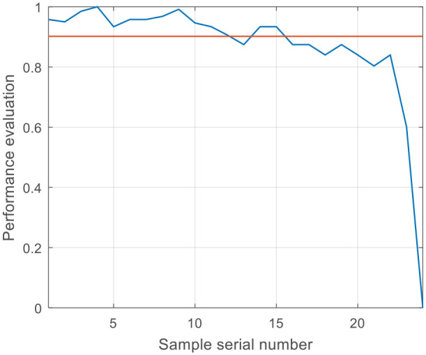
When establishing the performance degradation assessment model of VSFOA–CGWSVDD, the data of performance degradation stages are divided into two categories. One is eight groups of samples collected under the healthy state, which are called performance assessment health samples, and the other is 16 groups of samples, which are called performance degradation samples. First, the CGWSVDD hypersphere model is established with the healthy samples. Then, the CGWSVDD model is optimized with VSFOA. The comprehensive assessment of classification accuracy and minimum number of support vectors in the process of model training is taken as the fitness function of VSFOA. The initial values of population size, iteration times, and step factor are set as the same values as those of performance degradation assessment with simulation data mentioned in Section 4. The classification accuracy and evolutional generation of the VSFOA–CGWSVDD model is shown in Figure 9. The performance degradation process curve of the braking system obtained from the test sample is shown in Figure 10. Using the same method, the performance degradation curve of the GOA–SVDD model can also be obtained, as shown in Figure 11.

Figure 9.

The classification accuracy of VSFOA–CGWSVDD.

VSFOA–CGWSVDD: variable step-size fruit fly optimization algorithm–complex Gaussian wavelet support vector data description.

Figure 10.

The performance degradation curve of the braking system based on theVSFOA–CGWSVDD model.

VSFOA–CGWSVDD: variable step-size fruit fly optimization algorithm–complex Gaussian wavelet support vector data description.

Figure 11.

The performance degradation curve of the braking system based on the GOA–SVDD model.

GOA–SVDD: grid optimization algorithm–support vector data description.

From Figure 9, it can be seen that the optimal classification accuracy of 100% can be achieved in the 13th iteration in the VSFOA–CGWSVDD model, which shows the practicability of the VSFOA method.

As can be seen from Figures 10 and 11,

1. The performance of the braking system obtained by the VSFOA–CGWSVDD model and the GOA–SVDD model both show a trend of gradual degradation, which conforms to the law of equipment performance degradation.

2. Both models reach the adaptive performance degradation alarm threshold at the 13th simulation data, but the performance degradation curve based on the VSFOA–CGWSVDD model is better than that based on the GOA–SVDD model, and the early fluctuation is smaller.

Conclusion

According to the characteristics of the constant deceleration braking system, the pressure–time curve is selected as the characteristic data, and 29 features such as percentile, mean, RMS, and kurtosis factor are extracted to form the optional feature set. After feature selection, the performance degradation of the braking system is evaluated by the VSFOA–CGWSVDD method. The reliability and practicability of the VSFOA–CGWSVDD method are proved by simulation and experimental data. The main advantages of the proposed method are as follows:

1. A performance degradation assessment method based on correlation, monotonicity, and predictability is proposed in this article. First, the definitions of correlation, monotonicity, and predictability are given, and then, a comprehensive selection method of feature parameters based on expert scoring is proposed.

2. VSFOA is proposed. This method first searches in a large range with large step size and then gradually reduces the step size and search range with the increase of evolutional generation, so as to improve the search accuracy. This method is faster and more accurate than the classical VOA.

3. A performance degradation assessment method of VSFOA–CGWSVDD is proposed. The performance index is used to evaluate the overall performance of the braking system. The reliability of the proposed method is verified by the simulation data, and the practicability of the proposed method is verified by the data of the test bench. The performance index calculation method proposed in this article provides technical support for condition-based maintenance and intelligent maintenance of the hoist braking system.

The main disadvantages of this article are that there are fewer test data in the experimental verification, and the performance decreases only when the friction coefficient decreases. It cannot cover all the performance degradation states of the braking system. In order to achieve better performance degradation assessment results, it is necessary to gradually improve the database according to the performance analysis results in the operation. The VSFOA–CGWSVDD model runs slowly.

Author biographies

Juanjuan Li, PhD, Senior Engineer, School of Mechanical-Electrical Engineering, North China Institute of Science and Technology, China. Research Fields: Equipment Fault Diagnosis, Equipment Health Status Evaluation.

Guoying Meng, PhD, Professor, China University of Mining and Technology (Beijing), China. Doctoral Supervisor. Research Fields: System Dynamics, Test and Measurement Technology and Intelligent Instruments, Equipment Fault Diagnosis and State Detection, Fluid Drive and Control.

Jianguo Luo, PhD, Professor, School of Mechanical-Electrical Engineering, North China Institute of Science and Technology, China. Research Fields: Robotics Technology, Electromechanical Safety Technology.

Aiming Wang, PhD, Associate Professor, China University of Mining and Technology (Beijing), China. Research Fields: System Dynamics, Intelligent Instruments, Equipment State Detection.

Jun Ding, Lecturer, School of Mechanical-Electrical Engineering, North China Institute of Science and Technology, China. Research Fields: Fault Diagnosis of Machinery, Mechanical Seal Technology.

Wei Zhang, Senior Engineer, Luoyang Zhongzhong Automation Engineering Co., LTD. Research Fields: Automation Technology, Remote Equipment Monitoring Technology.

References

- 1.Liu J, Djurdjanovic D, Ni J, et al. Similarity based method for manufacturing process performance prediction and diagnosis. Comput Ind 2007; 58: 558–566. [Google Scholar]
- 2.Dang X, Jiang T. Degradation prediction based on correlation analysis and assembled neural network. J Beijing Univ Aeronaut Astronaut 2013; 39(1): 48–51. [Google Scholar]
- 3.Wang F, Chen X, Yan D, et al. Fuzzy C-means using manifold learning and its application to rolling bearing performance degradation assessment. J Mech Eng 2016; 52(15): 59–64. [Google Scholar]
- 4.Zhang L, Cao Q, Lee J, et al. PCA-CMAC based machine performance degradation assessment. J Southeast Univ 2005; 21(3): 299–303. [Google Scholar]
- 5.Jia X, Jin C, Buzza M, et al. Wind turbine performance degradation assessment based on a novel similarity metric for machine performance curves. Renew Energ 2016; 99: 1191–1201. [Google Scholar]
- 6.Wang G, Deb S, Coelho LDS. Earthworm optimisation algorithm: a bio-inspired metaheuristic algorithm for global optimisation problems. Int J Bio-Inspir Com 2018; 12(1): 1–22. [Google Scholar]
- 7.Wang L, Zhang L, Wang X-Z. Reliability estimation and remaining useful lifetime prediction for bearing based on proportional hazard model. J Cent South Univ 2015; 22: 4625–4633. [Google Scholar]
- 8.Shouqiang K, Yujing W, Lili C, et al. Health state assessment of a rolling bearing based on CFOA-MKHSVM method. Chin J Sci Instrum 2016; 13(9): 2029–2035. [Google Scholar]
- 9.Shuo Z, Ruilin B, Qinchuan L. Performance degradation assessment of rolling bearings based on Drosophila optimization algorithm-wavelet support vector data description. Chin Mech Eng 2018; 29(5): 602–608. [Google Scholar]
- 10.Zhen L. Research on performance degradation assessment method of reciprocating compressor. Kunming, China: Kunming University of Science and Technology, 2017. [Google Scholar]
- 11.Wang T, Yu J, Siegel D, et al. A similarity-based prognostics approach for remaining useful life estimation of engineered systems. In: International conference on prognostics and health management, Denver, CO, 6–9 October 2008, pp. 1–6. New York: IEEE. [Google Scholar]
- 12.Xi Z, Jing R, Wang P, et al. A copula-based sampling method for data-driven prognostics. Reliab Eng Syst Safe 2014; 132: 72–82. [Google Scholar]
- 13.Yan J, Koc M, Lee J. A prognostic algorithm for machine performance assessment and its application. Prod Plan Control 2004; 15(8): 796–801. [Google Scholar]
- 14.Wenzhu L. Integration of predictive maintenance strategy and production scheduling based on equipment degradation mechanism. Shanghai, China: Shanghai Jiao Tong University, 2011. [Google Scholar]
- 15.Yaogang H. Research on health monitoring and assessment method for key components of high power wind turbine. Chongqing, China: Chongqing University, 2017. [Google Scholar]
- 16.Hongbo C. Research on health diagnosis and risk assessment method of traction power supply system considering uncertainty. Chengdu, China: Southwest Jiaotong University, 2014. [Google Scholar]
- 17.Luoping P. Research on fault diagnosis system for hydroelectric generators based on health assessment and deterioration trend prediction. Beijing, China: China Academy of Water Resources and Hydropower Sciences, 2013. [Google Scholar]
- 18.Jian X. Research on state assessment and intelligent diagnosis method for hydropower units. Wuhan, China: Huazhong University of Science and Technology, 2014. [Google Scholar]
- 19.Bin Z. Data-driven performance degradation modeling and residual life prediction of mechanical equipment. Beijing, China: University of Science and Technology, 2016. [Google Scholar]
- 20.Xiaolong X. Research on aeroengine performance assessment and decline prediction method. Harbin, China: Harbin University of Technology, 2016. [Google Scholar]
- 21.Yi J, Deb S, Dong J, et al. An improved NSGA-III algorithm with adaptive mutation operator for Big Data optimization problems. Future Gener Comp Sy 2018; 88: 571–585. [Google Scholar]
- 22.Wang G, Tan Y. Improving metaheuristic algorithms with information feedback models. IEEE T Cybernetics 2019; 49(2): 542–555. [DOI] [PubMed] [Google Scholar]
- 23.Wang G, Guo L, Gandomi AH, et al. Chaotic Krill Herd algorithm. Inform Sciences 2014; 274: 17–34. [Google Scholar]
- 24.Wang G, Gandomi AH, Yang X, et al. A new hybrid method based on krill herd and cuckoo search for global optimisation tasks. Int J Bio-Inspir Com 2016; 8(5): 286–299. [Google Scholar]
- 25.Wang H, Yi J. An improved optimization method based on krill herd and artificial bee colony with information exchange. Memet Comput 2018; 10(2): 177–198. [Google Scholar]
- 26.Rizk-Allah RM, El-Sehiemy RA, Wang G. A novel parallel hurricane optimization algorithm for secure emission/economic load dispatch solution. Appl Soft Comput 2018; 63: 206–222. [Google Scholar]
- 27.Cui Z, Sun B, Wang G, et al. A novel oriented cuckoo search algorithm to improve DV-Hop performance for cyber-physical systems. J Parallel Distr Com 2017; 103: 42–52. [Google Scholar]
- 28.Wang G, Gandomi AH, Zhao X, et al. Hybridizing harmony search algorithm with cuckoo search for global numerical optimization. Soft Comput 2016; 20(1): 273–285. [Google Scholar]
- 29.Wang G, Deb S, Cui Z. Monarch butterfly optimization. Neural Comput Appl 2019; 31(7): 1995–2014. [Google Scholar]
- 30.Wang G. Moth search algorithm: a bio-inspired metaheuristic algorithm for global optimization problems. Memet Comput 2018; 10(2): 151–164. [Google Scholar]
- 31.Feng Y, Wang G. Binary moth search algorithm for discounted {0-1} knapsack problem. IEEE Access 2018; 6: 10708–10719. [Google Scholar]
- 32.Theodoridis S, Koutroumbas K. Pattern recognition & matlab intro. United States: Academic Press, 2010. [Google Scholar]
- 33.Chen Z, Cai Y, Jiang G. Research on support vector machine of complex gauss wavelet kernel function. Comp Appl Res 2012; 29(9): 69–71. [Google Scholar]
- 34.Li H, Guo S, Zhao H, et al. Annual electric load forecasting by a least squares support vector machine with a fruit fly optimization algorithm. Energies 2012; 5(11): 4430–4445. [Google Scholar]
- 35.Li M. Three-dimensional path planning of robots in virtual situations based on an improved fruit fly optimization algorithm. Adv Mech Eng 2014; 6: 314–797. [Google Scholar]
- 36.Shan D, Cao G, Dong H. LGMS-FOA: an improved fruit fly optimization algorithm for solving optimization problems. Math Probl Eng 2013; 2013: 108768. [Google Scholar]
- 37.Wang C. The relationship between the criteria and the number of measurements. J Changsha Electr Power Coll 1996(2): 73–74. [Google Scholar]
- 38.Juanjuan L, Guoying M, Aiming W, et al. Simulation platform for constant deceleration braking system based on Simulink. Aust J Mech Eng 2018; 16(Suppl. 1): 105–111. [Google Scholar]