

Abstract
This article proposes a conceptual model of a new type permanent magnet 3-degree-of-freedom motor. Its structure consists of an internal rotation module and a peripheral deflection module. It can be driven independently to achieve high-speed rotation and precise tilting of the motor. The 3-degree-of-freedom movement of the motor in space is achieved by the synchronous operation of the rotation and the deflection. In order to explore the loss problem caused by the temperature rise problem in the actual operation of the motor, the eddy current loss and core loss inside the permanent magnet of the motor are analyzed by theoretical formula and finite element method, respectively. Based on the static magnetic field, the gas flux density of two types of rotor permanent magnets in different coordinate systems is analyzed. The motor’s rotation and deflection torque characteristics are calculated using the principle of virtual displacement method. Using the auxiliary technology of the virtual prototype, according to the actual situation of the motor, the corresponding motion hinges and driving forms are summarized, and the control strategies of rotation, deflection, and rotation and deflection simultaneously are planned. The trajectory of the motor is described by observing the selected points. For the motor from product design to prototype testing and to the final processing assembly, a solid theoretical foundation is laid for the proposed work.
Keywords: Independent drive, cooperative control, electromagnetic loss, virtual prototype, air gap flux density
Introduction
For a long time, traditional motors have received widespread attention and research, but they can only achieve single-degree-of-freedom rotation. 1 In complex transmissions, the mechanical devices and multiple single-degree-of-freedom motors are required to complete multi-degree-of-freedom motion. 2 The motor in the coupling control system of this type tends to be bulky, slow in response, and poor in running stability, and the attitude tilting range and rotational eccentricity of the motor are reduced. 3 This urgently requires to center research on the model design and trajectory planning of multi-degree-of-freedom motors. 4 In addition, the material for manufacturing the permanent magnet is NdFeB, which not only has the advantages of high energy density, strong magnetism, and high electrical conductivity but also has disadvantages such as low Curie temperature and poor temperature performance. Therefore, it is necessary to analyze and study the eddy current loss and core loss generated when the motor is operated with multiple degrees of freedom. 5 At the same time, the torque characteristic is also an important performance index of the multi-degree-of-freedom motor. It is necessary to control the smoothness of the torque in each direction of the deflection and to avoid the fluctuation of the torque current to the greatest extent. In recent years, many experts at home and abroad have been working on the research of multi-degree-of-freedom motors. 6 D. Howe and others at the University of Sheffield in the United Kingdom have designed and developed a four-stage 3-degree-of-freedom spherical motor. The motor can realize a large deflection range with three axial angles of ±45° and output torque in a highly efficient manner. 7 Researcher Xia Changliang of Tianjin University, in order to further improve the three-dimensional magnetic field distribution performance of the motor, applies the magnetization method of the Halbach array to the permanent magnet spherical motor to obtain more. The air gap magnetic density is close to the sinusoidal trend. 8 A new type of permanent magnet 3-degree-of-freedom motor is now designed. Comparing the magnetization of permanent magnets in two different ways, the calculation principle is discussed by analytical method and solved by finite element method. 9 The internal eddy current loss and the core loss of the stator are calculated separately. 10 In order to verify the rationality of the rotor permanent magnet design, the radial component of the air gap magnetic density in the motor rotation module and the deflection module is studied. 11 The distribution law of axial electromagnetic torque and energizing current and azimuth angle is calculated based on the virtual displacement method, which proves the correctness of the stator winding’s energization strategy. 12 Using a unique classification mode, corresponding to two different control strategies according to their respective motion hinges and driving forms, the rotation motion and the deflection motion are separated. The rotor parts of the two types of motion are fixedly connected to a linkage body, so that the rotation and the yaw motion can also be cooperatively controlled.13–16 The axis motion of the motor deflection, the multi-azimuth skew motion, and the 3-degree-of-freedom motion are separately planned. The lower end of the rotor shaft is marked, the corresponding trajectory is viewed in the post-processing animation playback, and the kinematics and dynamics performance indexes are analyzed and researched. The control mechanism and motion state of the motor are further explained.17–20
Three views of the overall structure of the cooperative control permanent magnet motor model are shown in Figure 1, which are top view, left view, and front view, respectively. The isometric view along the X-Y angle bisector is shown in Figure 2. The structural parameters and rated data of the motor are shown in Table 1.
Figure 1.

Three views of the cooperative control motor.
Figure 2.

Isometric view of the motor x–y angle bisector.
Table 1.
Motor structure parameters and rated data.
| Parameter name | Parameter value |
|---|---|
| Rotation stator outer diameter (mm) | 105 |
| Deflection stator inner diameter (mm) | 52 |
| Rotation rotor outer diameter (mm) | 120 |
| Deflection rotor inner diameter (mm) | 70 |
| Rotational stator pole number Ns | 12 |
| Rotational rotor tooth number Nr | 8 |
| Deflection stator tooth number Ns | 8 |
| Deflection rotor tooth number Nr | 8 |
| Rated speed (r/min) | 30 |
| Rated power (W) | 400 |
| Rated torque (N) | 4 |
Analytical discussion and simulation calculation of electromagnetic loss
Principle of electromagnetic loss
The stator windings of the internal deflection module of the motor and the peripheral rotation module are connected with a three-phase power frequency alternating current, and the yoke generates an eddy current effect caused by the imbalance of the magnitude and orientation of the magnetic field and inside the hybrid-driven permanent magnet motor. The main factors of the eddy current loss of the outer rotor part are the magnetic field space, the current time, and the harmonic component of the winding back electromotive force. However, since the hybrid drive-type permanent magnet motor selects two different excitation coils, the inner stator and the outer rotor will rotate. The deflection permanent magnet is wrapped and enclosed in the rotor yoke, and when the inner and outer rotors of the motor are cooperatively controlled, the permanent magnets acting on the rotation and deflection modules are regarded as a built-in structure, and thus, the heat dissipation condition is poor. When the motor is performing three-degree-of-freedom motion in space, it is easy to cause local heating of the permanent magnet in the rotation and deflection module, which will cause the strong magnetic performance to be attenuated and even leads to increased risk of irreversible demagnetization as a whole, and the inner and outer rotor portions will also induce electromotive force and current is generated when the magnetic field lines are cut. The induced current flows through the stator core to generate core loss, and the copper loss generated after the stator winding of the motor is energized and heated. This has become a factor that cannot be ignored in the reliability and service life of the motor.
Select the NdFeB permanent magnet of NTP-336. The permanent magnet has the largest maximum energy product, and the remanence and coercivity are stronger than other brands of permanent magnets. Therefore, the anti-demagnetization ability is superior. In order to better solve the heat dissipation problem of the motor, the stator of the motor is made of silicon steel sheets, and the inside of the stator is provided with ventilation slots to improve the heat dissipation effect of the motor. When the motor runs stably at rated speed and rated load until the steady temperature rise of the motor, the maximum temperature is less than the maximum operating temperature Tω of the NTP-336 permanent magnet. A layer of zinc is electroplated on the surface of the permanent magnet to prevent oxidation of the permanent magnet and improve the anti-demagnetization capability of the permanent magnet.
Analytical method for eddy current loss of inner and outer rotor permanent magnets
According to Faraday’s law of electromagnetic induction, when the motor advances in rotation and deflection synchronously, the deflection permanent magnet, the yoke, and the support link perform continuous yaw and pitch motion internally. Cutting magnetic lines of force in the rotation module, rotating permanent magnets and yokes rotate at high speed on the outside. The magnetic lines of force of the deflection module are cut, and then, the permanent magnets corresponding to the induced electromotive force are generated on the corresponding module, and the induced current is formed as a closed loop of the conductive medium, which is regarded as eddy current phenomenon. The electromagnetic energy is generated by the induced current flowing in the permanent magnet, most of which is not output as mechanical energy with the movement of the rotor shaft, but is consumed inside the permanent magnet N and S stages, causing its temperature to rise.
Under the coordinated control of the current of the two windings, the induced electromotive force generated by the 3-degree-of-freedom movement of the rotor permanent magnet in the rotation and deflection magnetic fields emn, the air gap flux density of the N and S poles of the permanent magnet φmn, and the polar distance of the harmonic components τmn are, respectively, as follows
| (1) |
| (2) |
| (3) |
In the above equation, τr is the pole pitch at the time of the initial permanent magnet and hPM is the displacement amount of the magnetization direction of any radial magnetizing permanent magnet block grading.
The density We of the induced current in the eddy current field can be expressed as follows
| (4) |
σ is the conductivity of the radial magnetizing permanent magnet, demn is the fluctuation value of the induced electromotive force between adjacent nodes, and dl is the length between adjacent nodes.
The transient magnetic flux density that applies the m × n times harmonic in the electromagnetic field to the inside of the permanent magnet is decomposed in Fourier series as follows
| (5) |
Therefore, the eddy current loss density of the radial magnetizing permanent magnet is
| (6) |
Integrate the above single radial magnetizing permanent magnet
| (7) |
The total eddy current loss of the inner and outer rotor permanent magnets obtained by linear superposition is
| (8) |
Analytical calculation principle of iron loss of inner and outer stator yoke
The losses in the yoke of the stator section include eddy current loss , hysteresis loss , and abnormal loss , wherein the abnormal loss is an additional amount that may be considered in engineering consideration of iron loss. Its formula is as follows
| (9) |
The abnormal loss value is characterized by unit mass
| (10) |
In the above formula, f is the period of change of transient magnetic flux, Bm is the amplitude of transient magnetic flux, and α is the calculation parameter of abnormal loss.
Since the magnetization of the concentrated stator winding and the yoke is different, the loss of the corresponding portion is calculated separately based on the rotation and the alternating magnetic field generated by the concentrated stator winding. Using the longitudinal and tangential separation of the magnetic flux density, continue to calculate the following two losses
| (11) |
| (12) |
G and V0 are the material coefficient of the silicon steel sheet, S is the cross-sectional area thereof, and Br (t) and Bt (t) are the transverse and longitudinal components of the magnetic flux density.
After simplification, the total core loss value of the inner and outer stator yokes of the 3-degree-of-freedom motor can be expressed as follows
| (13) |
In the above formula, kc and ke are the coefficient values of eddy current loss and abnormal loss.
As shown in Figures 3 and 4, the different magnetization methods of a pair of N and S pole permanent magnets of the motor self-rotating module are compared. Obviously, the radial magnetized permanent magnets are in the same time period compared with the parallel magnetization of the permanent magnets. The magnetic flux density is slightly larger, and the magnetic lines of force are more evenly distributed around the annular permanent magnet.
Figure 3.

Magnetic density vector under parallel magnetization.
Figure 4.

Magnetically dense vector under radial magnetization.
The eddy current loss of the permanent magnet of the motor and the core loss of the stator yoke are shown in Figures 5 and 6, respectively. Take the 1 s duration of the smooth running phase of the motor. Compare the loss curves of the permanent magnets in different magnetization modes in the rotation and deflection modules. It is easily observed that the radial magnetization loss is based on the difference in the angles between the two different magnetization methods. The phase angle of the curve is 90° ahead of the loss curve of parallel magnetization. The eddy current loss of the parallel magnetized permanent magnet is about 4.8 W, which is slightly larger than the 4.5 W of the radial magnetization and the core loss curve. The amplitudes are approximately equal, about 60 W, but the core loss graph of parallel magnetization is worse than the sinusoidal trend of radial magnetization. The explanation clarifies the superiority and necessity of using radial magnetizing permanent magnets.
Figure 5.

Permanent magnet eddy current loss in different magnetization modes.
Figure 6.

Core loss in different magnetization modes.
Magnetic field characteristics analysis and simulation calculation
Because the new permanent magnet 3-degree-of-freedom motor has the structure of the inner and outer double fixed rotors, the magnetic field distribution is relatively complicated, and it is not easy to observe the obvious distribution law. Therefore, the models controlling the rotation motion and the yaw motion are separately distinguished. The finite element method is used to solve the air gap magnetic field with the only excitation source of the permanent magnet. According to Maxwell’s equation as shown in the following, the magnetic induction intensity B is the objective function
| (14) |
In the above equation, H(x, y, z) is the generalized magnetic field strength, B(x, y, z) is the generalized magnetic flux density, and J(x, y, z) is the current density in the vector form; it is divided into column vectors in the Cartesian coordinate system, and the vector product is added. The gas flux density can be expressed as follows
| (15) |
The x, y, and z components in the Cartesian coordinate system are transformed into the three components of (r, φ, θ) in the spherical coordinate system and (r, h, θ) in the cylindrical coordinate system according to the geometric relationship. The air gap flux density of the inner and outer rotor permanent magnets is extracted. The expression of its radial component is as follows
| (16) |
| (17) |
Among them, B1r is the air gap magnetic density of the deflecting portion and B2r is the air gap magnetic density of the rotating portion. Take a number of circles perpendicular to the Z-axis. Its radius fits the shape of the permanent magnet in the rotation and deflection modules and is equidistant from the permanent magnet in the horizontal direction. It is calculated by the software finite element method and superimposed, and the three-dimensional schematic diagram of the two types of hybrid driving in the static magnetic field is shown in Figures 7 and 8. The spatial distribution of the radial magnetic density Br of the outer rotor permanent magnet (spherical shape) along the Z-axis height h and the azimuth angle θ is perpendicular to the height of the XOY coordinate plane, centered on the origin, and the upper and lower range of the matching permanent magnet is ±25 mm. However, there is no significant periodic variation in the gas magnetic density of the outer rotor with increasing height. The range of the motor rotation within 1 week is 0°–360°, and the air gap magnetic density generally shows a distribution trend of sinusoidal function, and the maximum value of the magnetic field strength is about 0.12 T. However, due to the small gap between adjacent permanent magnets, mutual influence causes large harmonic components and poor sinusoidal. The spatial distribution of the radial magnetic density Br of the inner rotor permanent magnet (columnar) in the direction of angle A and azimuth angle B with respect to Z-axis is 180° with respect to the angle in the space. The range of the matching spherical permanent magnet is ±15°, but the angle with the Z-axis has little influence on the general trend of the air gap magnetic density. The azimuth angle is 0°–360° in one cycle of offset, gas. The radial component of the gap magnetic flux changes in a sinusoidal manner along the direction, with four peaks and four troughs, conforming to the structure in which the four permanent magnets are perpendicular to each other, appearing at 0°, 90°, 180°, and 360°. Its value is approximately ±0.2 T.
Figure 7.

Radial air gap magnetic density distribution of permanent magnets in deflection module.
Figure 8.

Radial air gap magnetic density distribution of permanent magnets in a self-rotating module.
Torque characteristic analysis and simulation calculation
Calculation principle of solving torque characteristics
Analysis of the torque characteristics of hybrid drive motor is critical to describing and controlling their 3-degree-of-freedom motion trajectories. In the calculation of torque, the virtual displacement method is adopted, that is, the entire electromagnetic system is assumed to be in a zero-loss energy storage state, and the instantaneous flux linkage of the displacement change is kept constant, and the total electromagnetic potential energy of the reserve is
| (18) |
In the above formula, V is the volume of the solution domain and H is the magnetic field strength under the solution domain.
Based on the virtual displacement concept, the rotation angle of the outer rotor along the latitude line is set to φ, and the deflection angle of the outer rotor along the longitude line is θ. The torques for controlling the rotation and yaw motion of the motor are
| (19) |
| (20) |
where Tφ is the torque component of the rotation along the latitude line, Tθ is the torque component of the yaw movement along the longitude line, and the interaction of the two drives the motor to complete the motion of 3 degrees of freedom.
Finite element method to calculate torque characteristics
The motor torque is analyzed by the finite element method, and the stator current is expressed by the magnetomotive force (amperes). In the transient electromagnetic field, an alternating current of three-phase power frequency is input into the stator coil that controls the rotation and deflection of the motor, and a rotating magnetic field is generated, thereby interacting with a constant magnetic field generated by the permanent magnet, so that stable transmission energy can be generated. Finally, the electromagnetic field–induced potential is cut by the rotor portion to generate electromagnetic torque. The characteristic surface as shown in Figure 9 of the electromagnetic torque generated by the hybrid drive motor around the three axes with the magnetomotive force and azimuth are analyzed. Both the external rotation motor and the internal deflection motor permanent magnet are radial magnetized, and the magnetomotive force of the stator coil is increased from 50 to 200 A.
Figure 9.

Three-dimensional surface map of motor rotation torque characteristics.
As can be seen from Figure 10, the deflection torque around the X-axis has a peak in the range of 60°–120°, a valley, and the peak is located at a position where A is equal to 91° and 108° and when the deflection angle is less than 10°. The deflection torque increases proportionally with the deflection angle. When the deflection angle is greater than 10°, the deflection torque decreases as the deflection angle increases until it approaches 0°. It can be seen from Figure 10 that the deflection torque is proportional to the magnetomotive force, that is, the deflection torque is proportional to the current of the stator coil.
Figure 10.

Three-dimensional surface map of the deflection torque characteristics of the motor around the X-axis.
As can be seen from Figure 11, the yaw deflection torque characteristic surface around the Y-axis is similar to that around the X-axis. The torque rises linearly in the range of 90° ± 10° and reaches a maximum value of 1.67 (N m) at 82° and 98°. Then, as the deflection angle increases, the torque gradually decreases, from 100° to 110°. In the range of 80°–70°, the decrease is slower. When the deflection angle exceeds 20°, the deflection torque rapidly decreases and is close to 0 when the deflection angle is 30°. It can be seen from Figure 11 that the deflection torque increases with the increase in the magnetomotive force, that is, the deflection torque increases as the current of the stator coil increases, and the deflection torque is proportional to the current of the coil. In a reasonable range, increasing the current of the stator coil can be used as one of the main means to improve the deflection torque of the deflection motor.
Figure 11.

Three-dimensional surface map of the deflection torque characteristics of the motor around the Y-axis.
Kinematics analysis of the rotation module
Drive control of rotation motion
The 3-degree-of-freedom motor rotation module includes an external output movable shaft, a cross-shaped support link connecting the start end of the output shaft and the motor casing, a concentrated winding for driving the rotation motion, a four-pair eight-pole annular permanent magnet of the rotation module, and a rotation module. The stator yoke is in the middle. In the peripheral rotation module of the multi-degree-of-freedom motor, the output shaft and the bearing base are selected as two objects, and the position point is selected as the midpoint of the ring connecting the output shaft and the cross support rod. A single-degree-of-freedom rotary motion around the Z-axis is created. The rotor output shaft is locked with its axis of rotation perpendicular to the working grid of the XOY plane to constrain the translational displacement on the three axes and the rotational drive in the X and Y directions. Figure 12 shows the rotation constraint pair and rotary drive of the motor’s external rotation module.
Figure 12.
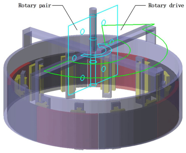
Outer rotor rotation rotary pair and rotary drive.
In order to verify the structural applicability and operational reliability of the designed hybrid drive motor, the control strategy of the start-up acceleration, smooth uniform speed, and brake deceleration of the virtual motor rotation operation is planned. It is expected that the motor will rotate at a speed of 300 r/min during the stable operation period of the rotation. The drive function around the Z-axis to the rotation pair is added and the acceleration as a function of time is taken as the variable. Specifying that the initial displacement and the initial speed are both 0, the motor starts to rotate at the static equilibrium position and stops during the final braking process. In the interactive simulation, the simulation time is set to 50 s, the number of steps is 500, and the angular velocity and angular acceleration of the center of mass point are loaded to the same graph, so as to visually observe the running condition of the motor rotation. As shown in the control strategy of Figure 13, the angular velocity corresponding to the center of mass point on the left scale is a red solid line, and the angular acceleration corresponding to the center of mass point on the right scale is a blue dotted line.
Figure 13.

Motor rotation part operation strategy.
Eccentricity analysis of the rotation motion of a rigid–flexible coupling system
In the classical theoretical mechanics, the multi-degree-of-freedom motion of the motor is not completely realistic considering the dynamics of the multi-rigid system. The rigid body is purely ideal, and it does not exist in practice. It only has the mass and rotational inertia parameters. Any two points on the component will not cause deformation, displacement, stress, strain, and rotor eccentricity at the free end of the motor. If the motor model is regarded as a rigid body member to solve the calculation, it is not accurate and cannot meet the accuracy requirements. Motor dynamics simulation often has distortion caused by excessive deformation during high-speed operation. Therefore, the kinematics and dynamics simulation of the rigid–flexible coupling system is optimally used to analyze the running condition of the motor. That is, after a part of the components are combined into a whole by a Boolean operation, the rigid body is used to flex it; the other part is still a rigid body, which is fixed to the node of the soft body. The external load is applied to the flexible body member to drive the rigid body to move, and the flexible external joint is set as a position of the rotating pair at the base as a point of interaction with the rotating pair and the driving, and the adjacent external point is taken at the same time. The unit area is rigid, releasing the translational freedom of the Z direction. The output shaft of the motor, the cross support link, and the annular spherical shell are made into a flexible body, as shown in Figure 14.
Figure 14.

Rotating pair and rotary drive of outer rotor under rigid–flexible coupling system.
Because in the classical theoretical mechanics, the multi-degree-of-freedom motion of the motor is not completely realistic with the dynamics of the multi-rigid system, the rigid body belongs to the pure ideal state. It does not exist in practice. It only has the mass and the inertia distance parameter. Any two points above will not cause deformation, displacement, stress, strain, and rotor eccentricity at the free end of the motor. If the motor model is regarded as a rigid body member to solve the calculation, it is not accurate and cannot meet the accuracy requirements, and the multi-flexible motor dynamic simulation often tends to be too large in high-speed operation, which leads to distortion. Therefore, the kinematics and dynamics simulation of the rigid–flexible coupling system is optimally used to analyze the running condition of the motor.
In the stage of smooth operation after the motor is started, the desired speed is 300 r/min and the frequency is 5 Hz. According to the sampling theorem, when the sampling interval f generated by the motor control simulation is greater than twice the time interval generated by the highest frequency fmax in the signal (f ⩾ 2fmax), the eccentric displacement of the multi-degree-of-freedom motor after sampling can be maximized. The data point information is retained in the limit without distortion. Therefore, in the interactive simulation control, starting from the starting position of the 3-degree-of-freedom motor model, the simulation step size is set to 0.1, that is, the simulation calculation time is 0.1 s. The simulation calculation frequency (sampling frequency) of the system post-processing is 10 Hz. Using the fast Fourier transform (FFT), the simulation running time of motor start → stable → braking is the independent variable. The sine wave frequency component of different frequencies is discretized in the time-domain form by the rotational speed planned by the multi-degree-of-freedom motor rotation module and then converted into the frequency domain form. The absolute value of the eccentric displacement of the returning rotor is set to the Y-axis component after the FFT is set. The FFTMag data point is only the left half of the spectrum, and the right side is mirror symmetrical. In the processing of a segment of the infinitely long sequence, the windowing function Hamming filtering can be used to more intuitively observe the attenuation between the main and side lobes of the amplitude–frequency characteristic. As shown in Figure 15, the X and Y component displacement curves of the motor deviating from the axis when rotating around the Z-axis are respectively subjected to FFT, and the generated FFT three-dimensional vibration curve is introduced into a frequency domain coordinate axis. The trend of the periodic variation of the offset of the two axes can be more stereoscopically reflected. The left color code is the gradient increment of the eccentric displacement.
Figure 15.

Deviation from the X-axis component vibration displacement during rotation.
As shown in Figure 15, the three-dimensional vibration image deviated from the X-axis during the motor rotation simulation operation, and it can be observed that the start-up and braking period are removed, and the eccentric displacement of the motor in the middle smooth running state is only at the frequency of 4.7–5 Hz. It is embodied and maintained at a constant value of approximately 0.008 mm. The remaining bands are almost zero. The three-dimensional vibration images of the two periods of starting acceleration and braking deceleration generally exhibit a bilateral symmetry trend at the time of 25 s, and the transition from the two sides to the middle is relatively smooth and stable, so only the 0–10 s of the motor starting acceleration on the left side is analyzed. During the period, there are three distinct sinusoidal trend attenuation vibrations. There is a sinusoidal variation of large displacement fluctuations in the first segment from 0 to 2.5 s. The peak of the sine wave corresponds to 2.5 Hz in the center of the left half of the spectrum, and the relative periodic variation is small. At this moment, the absolute value of the eccentric displacement of the rotating rotor portion reaches the maximum, about 0.0213 mm; the sinusoidal variation displacement fluctuation in the second stage of 2.5–4 s is slightly smaller than that of the first segment, and the peak of the sine wave corresponds to the 3.7 Hz of the left half spectrum. At this moment, the absolute value of the eccentric displacement of the motor is about 0.016 mm; the sinusoidal variation in the third segment is about 3.2–4.7 s. At about 10 s, the component of the eccentric displacement of the spectrum corresponding to the peak is about 0.013 mm. The motor eccentric absolute displacement is minimal. Finally, the corresponding spectrum in the time domain of 5–10 s is about 4–5 Hz, and the eccentric displacement of the fluctuation is also seen to be in the range of 0.0075–0.012 mm.Similarly, the three-dimensional vibration image deviating from the Y-axis when the motor is rotating is shown in Figure 16. The displacement in the steady and uniform state is not constant, but is increased from 0 to 0.006 mm in 10–24 s. It is ramped down from 0.006 to 0 mm during the 26–40 s period. The corresponding frequency is 5 Hz. The rotor eccentricity has the fastest periodic variation with respect to the Y-axis component displacement and is nearly zero within 24–26 s. Compared with the displacement from the X-axis, there is a big change in the transition from the start-up acceleration to the steady constant speed and the smooth uniform speed to the brake deceleration. Each has a large displacement, which is about 0.013 mm at 10 s. It is about 0.012 mm at 50 s. Similarly, due to the bilateral symmetry of the vibration image at the time domain, only the 40–50 s period of the right motor brake deceleration is analyzed. There are three obvious sinusoidal trend attenuation vibrations, and there is a larger one in the first segment of 0–2.5 s. For fluctuations, the maximum displacement is 0.01 mm. At the same time, it corresponds to the midpoint of the left half spectrum; the fluctuation in the second segment from 2.5 to 3.8 s is relatively small, and the number of periodic oscillations increases. The peak value of the sine wave is 0.008 mm, and the corresponding frequency is about 3.8 Hz. From the sinusoidal fluctuation of 3–5 s, the displacement amplitude is equal to the second segment, and the peak corresponding frequency is about 4.2 Hz. After that, when the motor is moving at a constant speed, there is another irregular arc rising fluctuation. The displacement value is about 0.01 mm.
Figure 16.

Deviation from the Y-axis component vibration displacement during rotation.
Discussion on iterative method for kinematics model of multi-degree-of-freedom motor
The multi-body mechanics simulation software is used to process the powerful functions of complex motion at high speed, constrain the operation law of mechanical system, and establish the mathematical model of mechanical kinematics of multi-degree-of-freedom motor to perform kinematics analysis. The drive in the existing motion pair is set, a complete constraint equation is constructed, a part of the degree of freedom of the component is released, a certain motion is generated, time-domain simulation of the rotation and yaw motion of the hybrid drive motor is performed, and the motor motion, constraints, speed, and acceleration are analyzed. The equation of motion is solved by an iterative method.
Set the number of all constraint equations to K (K= nh). Let , , and the static coordinate system in vector form all the constraint equations of the mechanical system
| (21) |
In formula (21), K represents a constraint. n is the number of degrees of freedom of any motion pair constraint, and h is the number of motion pairs of the system. is the Jacobian matrix, which is a square matrix of
| (22) |
The combination of all the drives and constraints that make up the motor’s rotation and deflection modules is
| (23) |
Let the starting speed be , and after deriving the above formula (23), the speed constraint expression of the rotor shaft of the motor is
| (24) |
Continue to derive the above equation (24), and the result is the acceleration constraint expression of the rotor axis
| (25) |
Let the initial acceleration be and substitute
| (26) |
In the interactive simulation operation of the virtual prototype, the high-speed spin and the tilt change caused by the precise tilt of the motor at any time can be solved by the Newton–Loveson method satisfying the iterative constraint as follows
| (27) |
In the formula, is the k time iteration.
In the post-simulation process, the kinematic analysis is quickly solved by the linear Calahan’s method for the driving forms such as displacement, velocity, and acceleration
| (28) |
| (29) |
Operation analysis in the deflection module
Constrained hinges and drive forms for yaw motion
The deflection module of the hybrid-drive-type 3-degree-of-freedom motor includes a yaw cross coupling, a square punching bushing, a four-pole eight-pair permanent magnet, two universal joints, a stator core, a stator bobbin, and a fixed support base. In the four-stator back yokes of the base, the motor deflection operation achieves two axial tilting movements by interlocking the output free ends of the two universal joints. The load relationship between the component and the component in the virtual prototype is set, the cross center axis as the support base is used as two moving parts, and the support base to the ground is fixed to create two universal joint hinges. The midpoint of the inner joint of the cross shaft is selected as a position point, and the direction is respectively along the positive direction of the X- and Y-axes and the two rotation axes of the negative direction of the X and Y axes, thereby constraining the degree of freedom of rotation around the Z-axis. The tilting motion based on the Z-axis XOY plane is realized, which ensures separate and independent control of the motor rotation module and the deflection module without mutual interference. The drive in the X- and Y-axes directions can be added to the motion pair of the corresponding universal joint hinge as follows: as seen in Figure 17, the motor internal deflection module has a universal joint tilt hinge and two axial rotational drives.
Figure 17.

Inner rotor deflection universal joint pair and rotary drive.
Control strategy for tilting along the axis
The motor is planned to be tilted based on the Z-axis deflection on the X- and Y-axes to drive the displacement as a variable, and the constraint inclination angle is 20°. The deflection around the X-axis and the Y-axis is set to drive the quantitative tilt with an accumulated Step function. Add a marker point at the center point of the ring at the end of the motor output shaft and define a local coordinate system on the global XOY plane. Fixing with the output shaft and moving together to observe the movement of the rotor part of the motor deflection module in the stator part, a cross-arc track centered on the static balance in the space is presented, and the rotation on the two axes movement is independent of each other.
The displacement measurements of the X and Y components at the end of the motor output shaft are created separately. The strip chart of the measurement process is displayed during the simulation run, and the trajectory of the marker point is observed after the simulation is completed. The motor completes the offset at the seventh time of the simulation run. The planned cross-arc path is shown in Figure 18, and the marked points of the X component reach the positive and negative displacement amplitudes at 5 and 7 s, respectively, and the marked points of the Y component reach the positive and negative displacement amplitudes at 1 and 3 s, respectively. The value is approximately 45.16 mm, and at this time, another displacement corresponding to the component is approximately zero.
Figure 18.

Offset trajectory of the motor along the axis and component displacement of X and Y.
Set the simulation duration to 8 s, the number of steps is 200, and the control strategy of the motor to deflect along the axis is to tilt 20° in the negative direction of the X- and Y-axes at 0–1 s, and return to the static equilibrium position at 1–2 and 2–3 s. Then tilt 20° in the positive direction of the Y-axis and return to the static equilibrium position after 3–4 s. The tilting displacement of the 4–7 s motor around the X-axis direction of the Y-axis is also the same, that is, the motor is tilted once every 2 s. The end time of the control simulation is 7 s, that is, it is stationary when the seventh motor is biased in the negative direction of the X-axis. The curve of the deflection angle as a function of time is shown in Figure 19.
Figure 19.

Offset angle of the motor along the axis within 0–7 s.
The average angular velocity of each tilt is 20 d/s. Figure 20 shows the angular velocity–time plot of the center of mass point of the rotor around the motor, and the integral in the range of the abscissa is the tilt angle of the motor in this range: 0, 1.5, 2.5, 3.5, 4.5, 5.5, 6.5, and 7.5 s. The absolute value of the angular velocity reaches a maximum of 30d/s centered on the static balance time of 4 s in the range of 0–7 s. The angular velocity time plots of the X and Y components within 8 s are bilaterally symmetric, and the drives on the two components do not interact.
Figure 20.

The angular velocity curve of the mass point of outer rotor.
As shown in Figure 21, the angular acceleration curve of the center of mass point has a large step mutation at the initial moment, rising from 0°/s2 to 100°/s2 and then accelerating to about 125° at intervals of 0.5 s. After that, the angular acceleration is decelerated to 0°/s2 at intervals of 0.5 s.
Figure 21.

The angular acceleration curve of the mass point of outer rotor.
The motor performs a 2-degree-of-freedom tilting operation under the action of a universal constrained joint and a rotary drive. The forward and reverse deflection angles of the specified limit are 20°, and the four poles and eight pairs of permanent magnets and the stator coils in the internal deflection module are kept at a certain displacement during the simulation duration of 8 s. Select the N and S pole permanent magnet cavity intersection line and match the center point of the stator coil to create a parallel X-axis minimum gap measurement, so as to observe the air gap length of the tilting motion in the Y-axis direction to the X-axis of the motor. The rotation angle is a reference, as shown in Figure 22; the abscissa is 70°–110°, and the rotation angle of the motor at its static equilibrium position is 90°. At this time, the corresponding air gap length is the smallest, about 6 mm. When the Y-axis is offset by ±20°, the corresponding rotation angles are 70° and 110°, and the maximum value is about 26.5 mm. At the same time, the displacement of the air gap lengths on both sides is symmetric with respect to the center point at the static equilibrium position, thereby verifying the motor’s symmetry and rationality of the design of the deflection part mode.
Figure 22.

Air gap length when the motor is offset along the axis.
Multi-angle tilt control strategy
In addition to the tilting along the axis, the motor deflection movement can also change the offset angle without changing the tilt displacement. Similarly, the simulation time is controlled to end at 145 s, that is, when the 145 s motor is biased to the negative direction of the Y-axis, it is stationary. As shown in Figure 23, it is more intuitive to observe the tilt of the multi-angle deflection of the motor, which proves the modeling accuracy and correctness of the deflection part of the 3-degree-of-freedom motor and provides more ideas for the subsequent study of the precise drive deflection of the motor.
Figure 23.

Motor multi-angle offset trajectory and component displacement of X and Y.
After the motor deflection portion returns to the origin after each offset, the next offset is performed at a 5° interval in the counterclockwise direction of the XOY plane in the axially decreasing displacement based on the Z-axis. This is used to make a reciprocating deflection motion for one cycle. In the simulation period of 146 s, the total deflection is inclined 72 times, and the displacement height in the Z-axis direction is about 128–135 mm under the action of driving displacement in the X and Y directions. The three-dimensional trajectory of the multi-angle offset of the motor is shown in Figure 24.
Figure 24.

Multi-angle tilted three-dimensional trajectory.
Take the point coordinate of the first offset of the motor for multi-angle tilt operation as the starting marker point, and then, take the same fixed point and the moving point as the middle and end marker points with the midpoint coordinates of the motor output shaft end and create a three-point type. The angle is measured in real time, and this is used as the abscissa variable. At the same time, the Z-axis translational displacement is taken as the ordinate dependent variable, and the simulation time is set to 38 s, that is, only the multi-angle value change of the tilt operation in the one-fourth cycle is observed. As shown in Figure 25, with the height of the output shaft at the static balance position corresponding to 135 mm and the right angle of 90°, the height of the Z-axis direction varies with the multi-angle tilt to exhibit a parabolic law, and the focal length corresponding to 0° is the largest. The 90° gradually decreases to 0°, and the amount of displacement each time descending by the arc is approximately equal, that is, the descending height of the multi-angle tilt is maintained at about 127 mm. In the multi-angle tilting operation within 90°, the motor has made a total of 19 reciprocating deflections. The angle values corresponding to each falling arc are about 5° apart, but the falling arcs in the middle of 5–12 times cannot be completely opposite. Corresponding angles of 20°–70° will have a certain deviation, and the trend of the 10th descending arc deviating from 45° is the largest, about 1°. The falling arcs on both sides are expected to have no corresponding deviations, and the last tilt is a straight line that is completely 90° above. It can be seen that the obtained coordinate fixed point value of the first tilting of 20° has a certain axial deviation from the obtained moving point coordinate of each tilting, and the partial deviation of the driving intersections in the X and Y directions is relatively obvious.
Figure 25.

Multi-angle offset by 5°.
As shown in Figure 26, the angular velocity/time curve of the outer rotor of the motor during multi-angle tilting movement can be seen by comparison. The curves of the two components are removed in 0~2s, 36~38s, 72~74s, 108~110s, 144~146s. The 5 periods of the 0-147s reaching the maximum angular velocity are independent of each other, and only during this phase, the motor performs the yaw operation in the positive and negative directions along the X- and Y-axes, and the angular velocity amplitudes on the X and Y components are also obtained here. It is ±30 d/s; the other four large-scale time periods have obvious intersections, showing the opposite sinusoidal variation law. When the angular velocity oscillation amplitude on the X component is increasing, the angular velocity oscillation amplitude on the Y component is correspondingly reduced. On the contrary, if the amplitude of the angular velocity oscillation on the X component is decreased, the amplitude of the angular velocity oscillation on the Y component is correspondingly increased. The rationality of the multi-angle tilting operation of the motor in different time periods is demonstrated from the side.
Figure 26.

Angular velocity/time at the center of mass point when the X- and Y-angle components are tilted at multiple angles.
The angular acceleration/time curve of the multi-angle tilting motion of the outer rotor is shown in Figure 27. It is easily observed that the general trend is similar to the angular velocity/time curve, and the overall trend is reversed. There are still small independent and large-scale intersections. During this period, the amplitude of the acceleration in the adjacent time does not completely follow the sinusoidal incremental decreasing law, but slightly up and down, and the degree of change of each fluctuation is more sharp, the response frequency is fast. The angular acceleration is maximized during positive and negative deflections, with an amplitude of approximately ±300 d/s2.
Figure 27.

Angular acceleration/time 2 at the center of mass point when the X- and Y-angle components are tilted at multiple angles.
Dynamic analysis of motor coordinated control
Motion constraint and torque application under cooperative control
As shown in Figure 28, three unidirectional moments Tor_X, Tor_Y, and Tor_Z with respect to the global XOY, the global XOZ, and the global YOZ coordinate system are, respectively, applied at the position point, and the directions are perpendicular to the working grids of the three coordinate planes. Among them, the torque around the Z-axis mainly realizes the rotation motion of the motor, and the torque around the X- and Y-axes mainly completes the orientation deviation of the motor.
Figure 28.

Illustration of three torques and ball joint with the bearing.
Analysis of dynamic performance under cooperative control
In order to reflect the 3-degree-of-freedom movement of the motor in space, a mode based on the start–stop control and smooth running of the motor when the rotation and the deflection are simultaneously performed is designed. Modify the quality characteristics of the motor and define the moment of inertia of the three spindles of the motor in user input mode
| (30) |
As shown in Figure 29, the angular velocity and angular acceleration/time curve of the absolute value of the combined component at the center of mass point after the three component drive torques are applied to the motor. The hybrid drive motor as a whole is similar to the motor rotation control strategy when it is in motion. It is divided into three stages: start acceleration, smooth uniform speed, and deceleration braking. The corresponding time periods are 0–20, 20–40, and 40–60 s. During the smooth and constant speed of the motor, the angular velocity reaches a maximum of 72°/s and the angular acceleration is 0. During the deceleration braking process, the angular acceleration rises from 0°/s2 to 5°/s2 in the 40–50 s. Within 50–60 s, it is always negative at 5°/s2. In the acceleration process, the torque on the X and Y components is sine and cosine trend that changes with time. It is not difficult to see that the angular acceleration is within 0–10 s. It is not a straight line parallel to the abscissa axis, but has a certain fluctuation and slope, but the general trend is the same as the angular acceleration curve of the deceleration braking process.
Figure 29.

The absolute value of the angular velocity and angular acceleration of the three combined components at the center of mass point of the motor.
Three-component drive torques are applied to the motor. The angular velocity and angular acceleration/time curve of the absolute value of the combined component is at the center of mass point. The hybrid drive motor as a whole is similar to the motor rotation control strategy when it is in motion. It is divided into three stages: start acceleration, smooth uniform speed, and deceleration braking. The corresponding time periods are 0–20 s, 20–40 s, and 40–60 s. During the smooth and constant speed of the motor, the angular velocity reaches a maximum of 72°/s and the angular acceleration is 0. During the deceleration braking process, the angular acceleration rises from 0 to 5°/s2 in the 40–50 s. Within 50–60 s, it is always negative at 5°/s2. In the acceleration process, the torque on the X and Y components is sine and cosine trend that changes with time. As shown in Figure 30, it is not difficult to see that the angular acceleration is within 0–10 s. It is not a straight line parallel to the abscissa axis, but has a certain fluctuation and slope, but the general trend is the same as the angular acceleration curve of the deceleration braking process.
Figure 30.

Three axial angular accelerations of the drive motor.
Three-degree-of-freedom motion trajectory analysis under cooperative control
The displacement of the cooperative control motor during the synchronous propulsion of the spin and tilting operation is shown in Figures 31 and 32. The translational displacement of the X and Y components is not obvious after the initial 5 s of the simulation, and then, it is not until the 55 s or so. The positive and cosine increasing oscillations are presented, which tends to be stable in the last 5 s of the simulation running stop. The displacement of the X component reaches the maximum at the end of the simulation, about 33 mm; the translational displacement of the Z component is in the first 10 s of the simulation. There is no obvious trend on the left and right, the modeling height of the motor output shaft is 135 mm, and then the trend of the convex arc similar to the quadratic function decreases in 10–50 s. In the last 10 s of the simulation run stop, the trend is similar to the ramp function and drops to approximately 132 mm. In contrast, it is not difficult to find that the height of the Z-axis up and down pitch varies from 0 to 3 mm under the action of rotation and yaw drive torque, which is much smaller than the width variation range of 0–33 mm based on the X- and Y-axes. That is, the motor output shaft makes a “spiral down” motion trajectory in space.
Figure 31.

Translational displacement of X- and Y-axes components in 3-degree-of-freedom motion.
Figure 32.

Translational displacement of the Z-axis component during 3-degree-of-freedom motion.
As shown in Figures 33 and 34, it can be seen that the end point of the output shaft draws a spiral-like trajectory in the playback of the resulting animation and simultaneously measures the angle between the three axes, and the angle between the X- and Y-axes starts from 90°. The change has almost no fluctuation in the first 5 s. After that, the apparent sinusoidal amplitude increase is changed. In the 10 s after the final brake deceleration, the oscillation frequency is obviously reduced due to the influence of the rotational inertia, and the fluctuation tends to be smooth. The angles at the end time are 75.54° and 84.49°, and the upper and lower fluctuation ranges of the X and Y axial angles are both 60° and 120°; the angle with the Z-axis changes from 0°. In the first 5 s or so, there is a more obvious increase in curvature. After that, it continues to increase with a certain slope, but with a small range of fluctuations. It is stable within 5 s of termination, and the angle at the end of the simulation is 14.79°. It can be seen that the angle of the three axial angles of the motor is approximately 15° when the 3-degree-of-freedom start–stop motion is performed in the space. Obviously, the inclination angle is reduced compared to the case that the motor is only deflecting, the three degrees of freedom motion speed of the motor is relatively slow in the specified time, and the rotation speed is only 8 r/min, so it is necessary to further improve the rotation and deflection simultaneously in accordance with the rotating speed.
Figure 33.

“Helical” motion trajectory and rotation angles in the X-, Y-, and Z-axes.
Figure 34.

“Spiral” trace.
In order to solve the problem that the motor is moving slowly in 3 degrees of freedom, the same control strategy is adopted to reduce the amplitude of the axial torque of the motor and the moment of inertia by reducing the length of the intermediate uniform speed. It can improve the speed of the motor when the rotation and deflection of the motor are running at the same time. As shown in Figures 35 and 36, it can be clearly seen that the “spiral” trajectory is more dense. The spiral motion path of the motor enables precise routing of the spherical arc surface. By setting the driving torque of the three axially different forms of the motor, it is also possible to complete various types of 3-degree-of-freedom movements at the center point.
Figure 35.

Motion trajectory and axial rotation angle after increasing the speed.
Figure 36.

“Spiral” trajectory after increasing the speed.
Experimental and simulation analysis
As shown in Figure 37, the power supply, digital signal processing (DSP) driver, displacement sensor, and physical prototype are used to form the detection platform. The end of the motor output shaft is equipped with a displacement sensor for detecting the running condition of the motor, and 10 A direct current (DC) is applied to the motor to be deflected. After the specified azimuth is stopped, the 3-degree-of-freedom trajectory of the motor is observed by an oscilloscope within a period of 1 s. As shown in Figure 38, in the hemispherical grid, the blue curve is the simulation data of the virtual prototype and the black curve is the experimental data of the motor. Obviously, the error between the two is small, further demonstrating the rationality and correctness of the motor control strategy.
Figure 37.
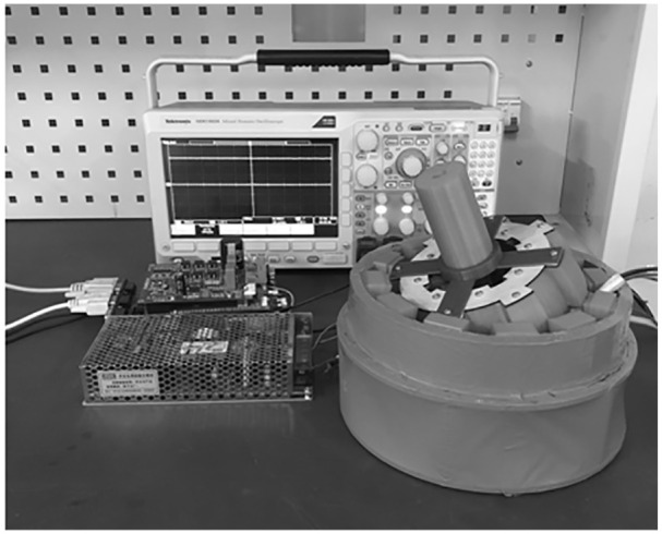
Experimental test platform for the motor.
Figure 38.

Comparison of simulation data and experimental data.
Conclusion
According to the designed permanent magnet hybrid drive 3-degree-of-freedom motor, the eddy current loss and winding copper loss of the permanent magnet of the motor are described in detail by analytical method. Then, in the different magnetization modes of the permanent magnets, the simulation calculation was carried out by the finite element method. The Maxwell and imaginary displacement methods in the finite element calculation principle are briefly discussed. Then, the radial magnetic density of the inner and outer rotors is analyzed in a constant magnetic field, and the relationship between the torque along the warp and weft and the energizing current of the coil is explained. The model of the virtual prototype is built by the three-dimensional (3D) mechanical design software, and the multi-body mechanics simulation software is imported. In the driving motor deflection module, it is divided into three operating phases of starting acceleration, smooth uniform speed, and braking deceleration. It demonstrates the stability and correctness of the motor rotation running control strategy. The variation of displacement on the X and Y components of the Z-axis when the motor rotates is studied. The FFT is used to generate the three-dimensional vibration image with the corresponding X and Y displacement changes. In the driving motor deflection module, the movement of the deflection part along the axis and the multi-angle tilting operation are designed, respectively, to realize the qualitative and quantitative calculation of the motor. Angle offset: during the 3-degree-of-freedom motion period of the motor, at the end of the simulation, the three axial angles are kept in the same range, which clarifies the accuracy of controlling the quantitative offset angle when the motor rotates in multiple directions. That is to say, in the movement mode of the hybrid-drive-type 3-degree-of-freedom motor, it has the characteristics of the start–stop control and the constant-speed operation of the rotation module and the advantage of the equal-variation inclination of the three axial angles of the deflection module.
Author biographies
Zheng Li received the B.Sc. and Ph.D. degrees in electrical engineering and power electronics and electric drive from Hefei University of Technology, Hefei, China, in 2002 and 2007, respectively. Since 2007, he has been a Lecturer, Associate Professor and Professor with the School of Electrical Engineering, Hebei University of Science and Technology. From July. 2013 to July. 2014, he has been a visiting scholar and part-time faculty in College of Engineering, Wayne State University, USA. His current research interests include design, analysis, and control of novel motors and actuators, intelligent control, and power electronics.
Lingqi Liu received the B.Sc. degree in electrical engineering and automation from Hebei University of Science and Technology, Shijiazhuang, China, in 2017. His research direction is the design and analysis of permanent magnet multi-degree-of-freedom motor.
Footnotes
The author(s) declared no potential conflicts of interest with respect to the research, authorship, and/or publication of this article.
Funding: The author(s) disclosed receipt of the following financial support for the research, authorship, and/or publication of this article: This work was supported by the National Natural Science Foundation of China (No. 51577048, 51877070, 51637001); the Natural Science Foundation of Hebei Province of China (No. E2018208155); the National Engineering Laboratory of Energy-saving Motor & Control Technique, Anhui University (No. KFKT201804); and Key Project of Science and Technology Research in Hebei Provincial Colleges and Universities (ZD2018228).
ORCID iD: Zheng Li  https://orcid.org/0000-0003-2383-7607
References
- 1.Li Z, Guo ZH, Zhang Y.Magnetic field analysis of a novel 3-DOF deflection type PM motor. J Hebei Univ Sci Technol 2012; 33(5): 422–428. [Google Scholar]
- 2.Li Z, Xue ZT, Sun KJ, et al. Electromagnetic system modeling and analysis of novel 3-DOF deflection type permanent magnet motor. Electr Mach Control 2015; 19(7): 73–80. [Google Scholar]
- 3.Li HF.3-D magnetic field analysis of a Halbach array PM spherical motor. Doctoral Dissertation, Tianjin University, Tianjin, China, 2008. [Google Scholar]
- 4.Li Z, Wang YT, Ge RL, et al. The summary and latest research of PM spherical M-DOF motor. Micromotors 2011; 44(9): 66–70. [Google Scholar]
- 5.Miao DM, Shen JX. Simulation and analysis of a variable speed permanent magnet synchronous generator with flux weakening control. In: Proceedings of the international conference on renewable energy research and applications, vol. 2, Nagasaki, Japan, 11–14 November 2012, pp. 1–6. New York: IEEE. [Google Scholar]
- 6.Wu FY, Yan XC. Kinematic and dynamics analysis for 3-DOF PM spherical motor. Mach Des Res 2017(3): 58–61. [Google Scholar]
- 7.Park HJ, Go SC, Lee HJ, et al. Application of co-ordinate transformation for 3-DOF motor’s vector control. Electron Lett 2013; 49(1): 31–32. [Google Scholar]
- 8.Quaid AE, Hollis RL. 3-DOF closed-loop control for planar linear motors. In: Proceedings of the IEEE international conference on robotics and automation, vol. 3, Leuven, 20 May 1998, pp. 2488–2493. New York: IEEE. [Google Scholar]
- 9.Li ZG.Detailed introduction and examples of ADAMS entry. Beijing, China: National Defense Industry Press, 2006. [Google Scholar]
- 10.Chen FH.ADAMS 2012 virtual prototyping technology from entry to proficiency. Beijing, China: Tsinghua University Press, 2013. [Google Scholar]
- 11.Zhai XC.Trajectory planning of three-degree-of-freedom permanent magnet spherical motor. Doctoral Dissertation, Tianjin University of Technology, Tianjin, China, 2017. [Google Scholar]
- 12.Cui ZB, Li HF, Yang K.Research on trajectory planning and obstacle avoidance technology of multi-degree-of-freedom spherical motor. Kexue yu Xinxihua 2016; (36). [Google Scholar]
- 13.Huang W, Zhan F, Zhao C.Cylinder-sphere 3-DOF ultrasonic motor and its control. Trans Nanjing Univ Aeronaut Astronaut 2004; 21(4): 272–276. [Google Scholar]
- 14.Li R, Wu FY, Zhang DQ, et al. Trajectory planning simulation of three-degree-of-freedom permanent magnet spherical motor. Comput Simul 2018; (4). [Google Scholar]
- 15.Smagt PVD, Grebenstein M, Urbanek H, et al. Robotics of human movements. J Physiol Paris 2009; 103(3–5): 119–132. [DOI] [PubMed] [Google Scholar]
- 16.Long P, Khalil W, Caro S.Kinematic and dynamic analysis of lower-mobility cooperative arms. Robotica 2015; 33(9): 22. [Google Scholar]
- 17.Zhang ZR, Yan YG, Su KC.No-load magnetic circuit calculation and 3D field analysis of tangential magnetic steel hybrid excitation synchronous motor. J Chin Electr Eng 2008; 28: 30. [Google Scholar]
- 18.Zhao J, Wang C, Zhao B, et al. A review of active management for distribution networks: current status and future development trends. Electr Power Comp Syst 2014; 42: 280–293. [Google Scholar]
- 19.Ji-Ming Z, Guang-Quan X, Shu-Kang C.The kinematics equation of three-degree-of-freedom motor with gimbals support. Micromotors 2010. [Google Scholar]
- 20.Goychuk I.Anomalous transport of subdiffusing cargos by single kinesin motors: the role of mechano-chemical coupling and anharmonicity of tether. Phys Biol 2015; 12(1): 016013. [DOI] [PubMed] [Google Scholar]