

Abstract
Fixed beam structures are widely used in engineering, and a common problem is determining the load conditions of these structures resulting from impact loads. In this study, a method for accurately identifying the location and magnitude of the load causing plastic deformation of a fixed beam using a backpropagation artificial neural network (BP-ANN). First, a load of known location and magnitude is applied to the finite element model of a fixed beam to create plastic deformation, and a polynomial expression is used to fit the resulting deformed shape. A basic data set was established through this method for a series of calculations, and it consists of the location and magnitude of the applied load and polynomial coefficients. Then, a BP-ANN model for expanding the sample data is established and the sample set is expanded to solve the common problem of insufficient samples. Finally, using the extended sample set as training data, the coefficients of the polynomial function describing the plastic deformation of the fixed beam are used as input data, the position and magnitude of the load are used as output data, a BP-ANN prediction model is established. The prediction results are compared with the results of finite element analysis to verify the effectiveness of the method.
Keywords: Fixed beam, deformation, load conditions, neural network, prediction model
Introduction
Fixed beams are widely used in various engineering applications, such as longitudinal beams in automobiles,1,2 track beams in gantry cranes,3,4 and wing beams in airplanes.5,6 Researchers have also performed many studies on these types of beams.7–9 In practical engineering applications, the fixed beam is often subjected to unknown external forces such as impact loads that can result in plastic deformations that often make it difficult to restore the beam to its original state. Because of the high cost of repair and reconstruction to mitigate this type of damage, the safety of human life can even be compromised. Therefore, structural reliability analysis is performed to ensure that these structures are properly designed to resist impact loads. 10 To do so, it is first necessary to accurately predict the impact load required to cause plastic deformation.
Many researchers have studied the large deformation of fixed beams and derived a considerable number of mathematical equations to describe their behavior accordingly.11,12 Wu et al. 13 studied the large rigid-elastic deformation problem of a three-dimensional beam element structure in aerospace applications and proposed a precise beam theory and finite element calculation equation for displacement. This equation was used for the modeling and analysis of highly flexible beam components in multibody systems undergoing very large static/dynamic rigid-elastic deformations. Dowell and McHugh 14 derived the Euler–Lagrange equations for a beam with a large deflection and provided the corresponding boundary conditions. Rezaiee-Pajand et al. 15 studied the three-dimensional deformation of curved circular beams under thermal-mechanical loading using the green function method to obtain their exact deformation. Tiar et al. 16 used the total Lagrangian approach to analyze the geometric nonlinear behavior of a two-dimensional fiber-reinforced elastic solid beam based on a four-node quadrilateral membrane composite element, then proposed a corresponding large-displacement finite element analysis method. Note that these studies primarily focused on the problem of beam deformation, established relevant models, and involved a large quantity of equation derivations.
The prediction of the deformation of objects is also a concern of many researchers.17–19 The primary deformation prediction methods used in such research include mathematical models and neural networks.20,21 Jang et al. 22 proposed a disc-spring model for the analysis of the elasto-plastic process of triangle heating and analyzed the deformation of a steel plate with the inherent strain method. To study the deformation behavior and microstructural evolution of heavy forgings, Necpal et al. 23 used the DEFORM 2D finite element modeling software and axisymmetric Lagrange method to predict the deformation of a precision seamless steel tube during cold drawing. Farokhi and Ghayesh 24 established a geometrically accurate continuous model of the center line rotation of a cantilever beam to predict its maximum vibration amplitude. Comparison of the results with those from a nonlinear finite element model verified that the accuracy of the established model for large cantilever beam deformations. Pham et al.25,26 studied the effects of plastic hinges and boundary conditions on the performance of reinforced concrete beams under slow-impact-velocity by numerical simulation. Furthermore, a method is proposed to predict the position of the stationary points, and compared with the experimental and numerical results, which proves the effectiveness of the method. In the field of actual engineering, intelligent algorithms are used by researchers in the field of damage prediction of engineering components.27,28 Chun et al. 29 proposed a method to quantify damage severity by use of multipoint acceleration measurement and artificial neural networks, which is accurate in damage identification and mechanical behavior prediction. Al Hussein et al. 30 used the historical records of London Bridge as training and test data, and artificial neural network is used to estimate the deterioration age for RC bridges based on deterioration data. Chun et al. 31 took I beam as the research object and proposed a three-step Random Forest method to evaluate various types of damage. Then, the accuracy of the proposed method is verified based on the results of a cross-validation and a vibration test of an actual damaged specimen. Ren et al. 32 developed a new machine (deep) learning calculation framework to determine and identify the damage loading parameters (conditions) of structures and materials according to the permanent or residual plastic deformation distribution or damage state of the structure. Quan et al. 33 used a backpropagation artificial neural network (BP-ANN) model with a temperature model to predict the compression deformation data of the Nimonic 80A superalloy.
Reverse engineering is a type of product design reproduction technology that extracts feature information from existing products to generate products with similar functions but that are not exactly the same. 34 As such, it offers a potential method for determining fixed-beam load and deformation state based on a set of model behavior parameters. At present, reverse engineering technology mainly obtains feature information from an original object and reconstructs a geometric model based on parameter feature information.35,36 In this manner, Wang et al. 37 used a 3D scanner to obtain characteristic information describing a model, adjusted a door panel surface processing according to the 3D scanning data, and proposed a new method of compensating for the spring back of the shaped piece. Chen et al. 38 proposed a machine learning method that predicted the position, velocity, and load duration of a rigid body impact on a hemispherical shell subject to permanent plastic deformation. Based on the permanent plastic deformation of the collision between a hemispherical elasto-plastic metal shell and an elastic material, the characteristic information is extracted as the input of deep learning, and the collision location, velocity and duration are obtained.
The referenced literature demonstrates that in order to describe the curve function of a beam element after deformation, a lot of mathematical calculation is usually needed. However, few researchers have investigated the prediction of the load magnitude and location based on fixed-beam deformation. As a result, it remains difficult to accurately reverse calculate the load and its position on the fixed beam from the observed deformation based on typical forward derivations used to calculate deformation based on the load characteristics. Therefore, based on the principle of reverse engineering, 39 this study establishes the relationship between load magnitude and location and beam deformation information using a neural network model, then carries out the reverse solution to determine the applied load from the curvature. Using these results, a prediction algorithm is proposed in this study to determine the load magnitude and location on a fixed beam exhibiting plastic deformation in a single dimension, and its accuracy is confirmed against the results of finite element simulations.
Finite element model of a fixed beam
Model parameters
In this study, a finite element analysis model was evaluated in which the two ends of a one-dimensional beam are completely fixed as shown in Figure 1. A series of loads were applied to these model produce plastic deformations in the beam. The one-dimensional fixed-beam model is shown in Figure 1, in which the length of the beam is , the beam section width and height are 2 mm, the left fixed end is point , the midpoint is point , and the right fixed end is point . The beam section is 2 mm square. The beam was divided into 50 equal micro-segments to analyze the finite element model. The material used for the one-dimensional fixed-beam model was a high-strength, bake-hardening steel, the basic properties of which are shown in Table 1. 40 Where, density , young’s modulus , poisson ratio , yield strength , tensile strength , uniform elongation , and maximum elongation .
Figure 1.

One-dimensional fixed-beam model.
Table 1.
Material properties of fixed-beam model.
| Elastic properties | Plastic properties | ||
|---|---|---|---|
| 7850 | 238 | ||
| 210 | 373 | ||
| 0.3 | 23% | ||
| 38.2% | |||
Model loading
For the one-dimensional fixed-beam model, different points were selected at which a concentrated load was applied to produce plastic deformation. As can be observed in Figure 1, the principle of symmetry means that points on only one side of the midpoint of the beam need to be analyzed. The state of the one-dimensional fixed beam before inducing deformation is shown in Figure 2. Points and are connected along the X-axis, and the direction perpendicular to the X-axis at point is taken as the Y-axis. A Point on the beam is then defined at , where applying a concentrated load causes a large plastic deformation in the positive Y-axis direction. Thus, the coordinates of each point after deflection are , , and , as shown in Figure 3. The commercial finite element analysis package Abaqus 6.14 from Dassault Systèmes was adopted for the finite element analysis, and using 6 Core Interl Xeon W-2133, 32 Gb Think Station with Windows 10 application were performed at laboratory. This is an example of the process of the finite element analysis, with other results as shown in detail in the four models in Figure 4.
Figure 2.

State of a one-dimensional fixed beam before deformation.
Figure 3.

State of one-dimensional fixed beam after deformation due to load applied at point .
Figure 4.

Example deflection diagrams of finite-element analysis models. (a) The first example of model analysis. (b) The second example of model analysis. (c) The third model analysis example. (d) The fourth model analysis example.
A total of 50 points were equally spaced along the segment in Figure 1, labeled as points at which a concentrated load was applied using the loading process shown in Figure 5. The minimum value of the concentrated load was set to and increased to a maximum value of in intervals, labeled as loads . As each point was loaded with each load, a total of 500 sample models were obtained. When a small load was applied in the highly rigid portions of the fixed beam near its end points, its maximum deformation was less than 0.1 mm in 24 load cases. These cases were removed by manual screening, resulting in 476 remaining samples.
Figure 5.
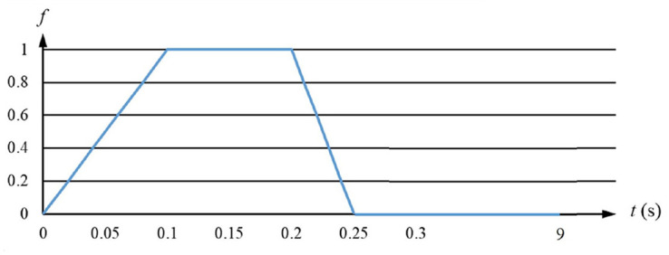
Amplitude of concentrated load application over time.
Function fitting of fixed-beam deformation curves
A polynomial is a simple continuous function that fits curves quite well as its geometric characteristics are smooth. Accordingly, in this study, we chose to use a polynomial to fit the one-dimensional fixed-beam deformation curve. The polynomial expression for the fitted curve is as follows:
| (1) |
where is the coefficient of polynomial expression and is coefficient of , .
Commonly used indicators to evaluate the fit of a function to a curve include:
(1) Root mean squared error (RMSE): This statistical parameter is the standard deviation of the regression system. 41 The closer the RMSE is to zero, the more accurate the data is fitted. The RMSE is calculated by:
| (2) |
where is the predicted value of the fitted function, is the value of the original data, is the number of calculated data points, and is an integer in the set denoting each compared point.
The RMSE method based on the error between the predicted and original values. The indicators that represent the quality of fit of the curves can also be evaluated in such a way that all errors are relative to the average of the original data as follows:
(2) R-squared (R2): This statistical parameter is defined as the ratio between the sum of the squares of the regression (RSS) and total sum of squares (TSS)42,43 as follows:
| (3) |
where
| (4) |
| (5) |
and is mean value of the original data points.
The R2 value represents the overall quality of fit of the data. It can be observed in equations (3)–(5) that R2 has a normal value range of [0,1], in which a value closer to one represents a stronger ability of the equation to reflect the value of . 44
This model is also good for data fitting. Generally, the requirement for good correlation is that R2 is greater than 0.9. In order to generate a polynomial fitting function that can not only fit the deformation curve well, but also ensure that the calculation is not too complicated, a suitable highest power n must be identified. In this study, all the models used to fit the data were developed to provide R2 values greater than 0.995. When all model fittings satisfied this requirement, the minimum value of n was eight. Therefore, this study selected an eighth-power polynomial function to fit the deformation curves. Four examples of the resulting polynomial fitted curves compared to the data are shown in Figure 6.
Figure 6.

Eighth-power polynomial function fitting examples. (a) The first example of function fitting. (b) The second example of function fitting. (c) The third function fitting example. (d) The fourth example of function fitting.
To evaluate the fitted curves according common indicators RMSE and R2 above, 40 samples were randomly selected, and the RMSE and R2 values were calculated. The results, shown in Figure 7, indicate an average RMSE value of 0.11149 and average R2 value of 0.9968. Therefore, the use of the polynomial function satisfies the accuracy requirements, and the polynomial expression of the fitted curve can be defined as:
Figure 7.
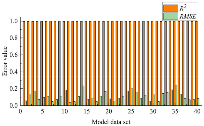
Fitting function evaluation results.
| (6) |
Prediction algorithm design, implementation, and verification
In this study, an algorithm flow for predicting the load magnitude and location resulting in a given plastic deformation of a one-dimensional fixed beam was designed as shown in Figure 8. Of these samples, 400 were randomly selected as training samples, and 40 of the remaining 76 cases were randomly selected as testing samples for the neural network.
Figure 8.

Flow chart of the prediction algorithm for the large deformation of a fixed beam.
Neural network design
An artificial neural network (ANN) is a computational network with a structure that simulates biological neurons to learn the relationship between input data and output data, and is a very effective tool for predicting output data when a large set of training data are given. A typical ANN consists of types of three layers: the input layer, hidden layers, and output layer. The input layer receives external data, the hidden layers provide a complex network structure to simulate the nonlinear relationship between the input data and output data, and the output layer generates the output data. 45 A BP-ANN is a multilayer feedforward network trained by error back propagation, and is frequently used to address complex nonlinear relationships between multiple variables.46–48 Its basic principle is the gradient descent method, which uses gradient search technology to minimize the target error of the actual output value of the network against the expected output value.
In this study, the relationship between the magnitude and position of the applied load and the coefficient of the polynomial function of the curve was determined using the BP-ANN. Because the model object is a one-dimensional beam element, there is one load magnitude parameter and one load location parameter , resulting in a neural network layer with two nodes. In this study, the polynomial function expression in equation (7) was used to express the plastic deformation of the fixed beam. As the highest power of the polynomial function used to fit the curve was eight, there are nine potential polynomial coefficients , introducing another network layer with nine nodes. Thus, there were four layers in the proposed neural network model: one input layer, one output layer, and two hidden layers.
Training sample neural network
An initial neural network was trained using the 400 models generated and selected as detailed in Section 2.2. At this time, there were two input nodes ( and ), the output layer of the neural network consisted of , and there were two hidden layers with 20 nodes each. The required training accuracy was . This training sample neural network is shown in Figure 9.
Figure 9.

Training sample neural network.
The training steps for the initial neural network were as follows:
Develop input: Collect 400 training samples to construct the relationship model between the load magnitude and location as the input layer and the polynomial coefficients as the output layer.
Construct the BP-ANN and set network parameters: Set the number of neural network layers to four: one input layer, two hidden layers, and one output layer. The input layer of the neural network consists of two nodes: the load magnitude parameter and the load location parameter. The output layer consists of the polynomial function coefficients, making nine nodes. The number of hidden layer nodes is set to 20.
Set training parameters and train the network: Set the training accuracy requirement to , and the minimum gradient to .
Run the BP-ANN and evaluate the data processing accuracy of the established initial neural network model.
The training results are shown in Figure 10, in which it can be observed that after 16 epochs, the relative standard deviation of the training set is 0.99769 and the training accuracy reaches . The provided training accuracy thus meets the expected training accuracy requirements, indicating that the initial model is reasonable.
Figure 10.

Training results of the iteration calculation of the initial neural network.
As the above results demonstrate, the initial neural network training indicated a good fitting effect. Sample expansion was then performed based on Latin hypercube Sampling (LHS) to increase the number of samples input into the neural network from 400 to 2000. 49 Then, the data from the initial neural network was used to evaluate and capture the relationships within the expanded data set as detailed in Section 4.3.
Neural network for load magnitude and location prediction
A neural network for load magnitude and location prediction was trained using the 2000 samples. To then predict the load magnitude and location resulting in the observed plastic deformation of a one-dimensional fixed beam, the input layer of the neural network contained nine nodes ( ) determined by the training set. The output layer continued two nodes ( and ). Again, there were two hidden layers with twenty nodes each. The resulting predictive neural network shown in Figure 11 was then trained to capture the relationship between load magnitude and location and the one-dimensional fixed-beam deformation.
Figure 11.

Neural network for predicting load magnitude ( ) and location ( ).
The training and validation steps of the predictive neural network were as follows:
Develop input: Obtain 2000 training samples by expanding the initial 400 samples based on LHS in order to construct a more accurate relationship model between the polynomial coefficients of the input layer and load magnitude and location of the output layer.
Construct the BP-ANN and set network parameters: The number of neural network layers was set to four: one input layer, two hidden layers, and one output layer. The input layer consists of the nine polynomial function coefficients as nodes. The output layer consists of two nodes, the load magnitude parameter and load location parameter. Again, there are 20 nodes in each of the two hidden layers.
Set training parameters and train the network: Set the maximum number of training steps to , the training accuracy to , and the minimum gradient to .
Run the BP-ANN and evaluate the established predictive neural network model based on the expanded sample set.
The results are shown in Figure 12, in which it can be seen that after 93 epochs, the relative standard deviation of the training set is 0.99761 and the training accuracy is 0.0014527, indicating that the predictive neural network is well-fit to the results. The prediction and verification of the stress point of the fixed beam under large deformation can accordingly be carried out with confidence.
Figure 12.

Prediction results of the iterative calculation of the neural network.
In this study, 40 sets not used in the training sets to evaluate the predictions of the trained neural network. The load magnitude and location relative errors and , respectively, of the prediction results were calculated to confirm that they were less than established error parameter , which was set to 10%. Using the polynomial fitting expression coefficients of the deformed one-dimensional fixed-beam shape as the input of the neural network, the load magnitudes and locations predicted by the neural network, as detailed previously in this section, were compared with the actual values originally input into the finite element model data to generate the fitting expressions, as detailed in Section 2. A comparison of the algorithm-predicted and finite-element determined actual load magnitudes and locations for the plastic deformation of a one-dimensional fixed beam for all 40 sample datapoints is shown in Figure 13.
Figure 13.

Comparison of the algorithm-predicted and finite-element determined actual load magnitudes and locations for the plastic deformation of a one-dimensional fixed beam.
To more closely analyze the prediction results in Figure 13, the relative and average errors of the predicted load magnitude and location were calculated by, respectively:
| (8) |
| (9) |
where is the predicted load magnitude or location, is the actual load magnitude or location, and k is the iteration number in the integer set ( ), in which is the total number of iterations.
The errors calculated by equations (8) and (9) are shown in Figure 14. The maximum relative and average error of the predicted load location is and , respectively. The maximum relative and average error of the predicted load magnitude is and , respectively. Some of the reasons for the large errors in prediction results may be caused by the lack of initial samples and some errors in the extended samples. The relative load magnitude and location errors and , respectively, are both smaller than the set error , confirming the accuracy of the predictive algorithm. These results indicate that the BP-ANN-based prediction algorithm proposed in this study can be used to predict the magnitude and location of the load required to produce a given plastic deformation of a one-dimensional fixed beam.
Figure 14.

Relative errors of predicted load magnitude and location.
Conclusions
This study addresses the difficulty of determining the location and magnitude of a load on a fixed beam necessary to cause plastic deformation. A load magnitude and location BP-ANN prediction algorithm based on the series of finite element models of highly deformed one-dimensional fixed beams was accordingly constructed based on the principles of reverse engineering. The BP-ANN was initially trained using a set of 400 applied load magnitudes and locations to capture their relationships to their associated deformations as described by the coefficients of a polynomial fitting curve function. The training sample set was then expanded to 2000 items based on LHS to train the BP-ANN to predict load magnitude and location based on these coefficients. The accuracy of the load magnitudes and locations predicted by the proposed algorithm was then confirmed by comparison to the results from the finite element models. The results of this study can be summarized as follows:
Based on the analysis of the plastic deformations of a one-dimensional fixed-beam finite element model, a polynomial function fitting expression was derived to describe deformation geometry. This provided a quantitative description of plastic deformation that could be used as input to the BP-ANN.
Using the principle of reverse engineering, a BP-ANN was forward trained on a set of finite element modeling data samples to predict the polynomial coefficients describing deformation based on load magnitude and location. Then, more loads and positions are extracted as the input of the forward BP-ANN based on the LHS, the data set of the reverse training sample is expanded, and the reverse training is performed. This approach effectively addresses the problem of insufficient neural network samples under normal circumstances.
To predict the load magnitude and location required to produce plastic deformation in a one-dimensional fixed beam, an algorithm flow with high reliability was proposed. The load magnitudes and locations predicted by the algorithm and provided by the finite element analyses were compared, confirming the accuracy of the algorithm. The prediction algorithm proposed in this study thus provides a promising new approach for determining the load magnitude and location required to produce plastic deformation in a rigid body.
For further studies, we will develop models using different beam supports and large beam cross-sectional areas, and extend the model to 2D and 3D scenarios for research. The method proposed in this paper is used to analyze the cause of plastic deformation of the beam and determine the initial collision conditions. In engineering practice, the permanent plastic deformation of the general beam is known, but the load is unknown. According to actual data, the method can be used to obtain the precise size and position of the collision load, which has important practical significance. For example, the deformation of the longitudinal beam in the car, the accurate collision load and position, can help the traffic police determine the responsibility for the accident. The deformation of the beams of the bridge and the accurate collision load and location can help designers and construction personnel repair the bridge. The deformation conditions in the rail beam of the gantry crane and the wing spar of the aircraft can obtain accurate collision load and position, which can help designers improve the level of product design.
Author biographies
Junqing Yin is currently a Lecturer with the Xi’an Polytechnic University. His research interests include advanced assembly technology and functional composite materials.
Jinyu Gu is currently conducting his Master degrees in Xi’an Polytechnic University. His research interests include advanced assembly technology and functional composite materials.
Yongdang Chen is currently a Professor with the Xi’an Polytechnic University. His research interests include computer integrated manufacturing (CIMS), enterprise information engineering technology, knowledge management, and knowledge engineering.
Wenbin Tang is currently an Associate Professor with the Xi’an Polytechnic University. His research interests include tolerance analysis, tolerance allocation, digital design, and computer- aided design.
Feng Zhang is currently an Associate Professor with the Northwestern Polytechnical University. His research interests include aircraft reliability engineering and sensitivity analysis.
Footnotes
The author(s) declared no potential conflicts of interest with respect to the research, authorship, and/or publication of this article.
Funding: The author(s) disclosed receipt of the following financial support for the research, authorship, and/or publication of this article: Authors gratefully appreciate the support of Xi’an key laboratory of modern intelligent textile equipment (2019220614SYS021CG043), Natural Science Foundation of Shaanxi Province (2019JM-377), Postgraduate Tutor guidance ability improvement plan at Northwestern Polytechnical University (2019), China National Textile and Apparel Council (2019061) and Science & Technology Research Program in Xi’an City (2020KJRC0017).
ORCID iD: Feng Zhang  https://orcid.org/0000-0003-2987-8418
References
- 1.Wang H, Xie H, Cheng W, et al. Multi-objective optimisation on crashworthiness of front longitudinal beam (FLB) coupled with sheet metal stamping process. Thin-Walled Struct 2018; 132: 36–47. [Google Scholar]
- 2.Gao D, Zhang N, Feng J. Multi-objective optimization of crashworthiness for mini-bus body structures. Adv Mech Eng 2017; 9(7): 1–11. [Google Scholar]
- 3.Gening X, Yanfei T, Wenju L. Research on U type gantry crane structure parametric finite element analysis system based on C# and APDL. Adv Eng Res 2017; 113: 611–618. [Google Scholar]
- 4.Kulka J, Mantic M, Fedorko G, et al. Analysis of crane track degradation due to operation. Eng Fail Anal 2016; 59: 384–395. [Google Scholar]
- 5.Qiu L, Yuan S, Mei H, et al. An improved Gaussian mixture model for damage propagation monitoring of an aircraft wing spar under changing structural boundary conditions. Sensors 2016; 16(3): 291. [DOI] [PMC free article] [PubMed] [Google Scholar]
- 6.Bruce RR. Initial and progressive failure analysis of a composite wing spar structure. J Mech Eng 2017; 14(2): 167–183. [Google Scholar]
- 7.Lee P-S, McClure G. A general three-dimensional L-section beam finite element for elastoplastic large deformation analysis. Comput Struct 2006; 84(3–4): 215–229. [Google Scholar]
- 8.Challamel N, Reddy JN, Wang CM. Eringen’s stress gradient model for bending of nonlocal beams. J Eng Mech 2016; 142(12): 04016095. [Google Scholar]
- 9.Luo Y, Bao J. A material-field series-expansion method for topology optimization of continuum structures. Comput Struct 2019; 225: 106122. [Google Scholar]
- 10.Zhang F, Xu X, Cheng L, et al. Mechanism reliability and sensitivity analysis method using truncated and correlated normal variables. Safe Sci 2020; 125: 104615. [Google Scholar]
- 11.Beheshti A. Large deformation analysis of strain-gradient elastic beams. Comput Struct 2016; 177: 162–175. [Google Scholar]
- 12.Chen G, Bai R. Modeling large spatial deflections of slender bisymmetric beams in compliant mechanisms using chained spatial-beam constraint model. J Mech Rob 2016; 8(4): 041011. [Google Scholar]
- 13.Wu G, He X, Pai PF. Geometrically exact 3D beam element for arbitrary large rigid-elastic deformation analysis of aerospace structures. Finite Elem Anal Des 2011; 47(4): 402–412. [Google Scholar]
- 14.Dowell E, McHugh K. Equations of motion for an inextensible beam undergoing large deflections. J Appl Mech 2016; 83(5): 051007. [Google Scholar]
- 15.Rezaiee-Pajand M, Rajabzadeh-Safaei N, Hozhabrossadati SM. Three-dimensional deformations of a curved circular beam subjected to thermo-mechanical loading using greens function method. Int J Mech Sci 2018; 142–143: 163–175. [Google Scholar]
- 16.Tiar A, Zouari W, Kebir H, et al. A nonlinear finite element formulation for large deflection analysis of 2D composite structures. Compos Struct 2016; 153: 262–270. [Google Scholar]
- 17.Li Y, Wang K, Jin Y, et al. Prediction of welding deformation in stiffened structure by introducing thermo-mechanical interface element. J Mater Process Technol 2015; 216: 440–446. [Google Scholar]
- 18.Ba M, Tinjum JM, Fall M. Prediction of permanent deformation model parameters of unbound base course aggregates under repeated loading. Road Mater Pavement Des 2015; 16(4): 854–869. [Google Scholar]
- 19.Sun X, Han J, Crippen L, et al. Back-calculation of resilient modulus and prediction of permanent deformation for fine-grained subgrade under cyclic loading. J Mater Civil Eng 2017; 29(5): 04016284. [Google Scholar]
- 20.Wang L, Si H. Machining deformation prediction of thin-walled workpieces in five-axis flank milling. Int J Adv Manuf Technol 2018; 97(9–12): 4179–4193. [Google Scholar]
- 21.Pham TM, Hao H. Prediction of the impact force on reinforced concrete beams from a drop weight. Adv Struct Eng 2016; 19(11): 1710–1722. [Google Scholar]
- 22.Jang CD, Kim TH, Ko DE, et al. Prediction of steel plate deformation due to triangle heating using the inherent strain method. J Mar Sci Technol 2005; 10(4): 211–216. [Google Scholar]
- 23.Necpal M, Martinkovič M, Buranský I. Deformation prediction and Finite Element Analyses of precision seamless tubes during cold drawing. MATEC Web Conf 2017; 137: 05005. [Google Scholar]
- 24.Farokhi H, Ghayesh MH. Geometrically exact extreme vibrations of cantilevers. Int J Mech Sci 2020; 168: 105051. [Google Scholar]
- 25.Pham TM, Hao H. Effect of the plastic hinge and boundary conditions on the impact behavior of reinforced concrete beams. Int J Impact Eng 2017; 102: 74–85. [Google Scholar]
- 26.Pham TM, Hao H. Plastic hinges and inertia forces in RC beams under impact loads. Int J Impact Eng 2017; 103: 1–11. [Google Scholar]
- 27.Abdeljaber O, Avci O, Kiranyaz MS, et al. 1-D CNNs for structural damage detection: verification on a structural health monitoring benchmark data. Neurocomputing 2018; 275: 1308–1317. [Google Scholar]
- 28.Mariniello G, Pastore T, Menna C, et al. Structural damage detection and localization using decision tree ensemble and vibration data. Comput–Aided Civ Infrastruct Eng. Epub ahead of print 11November2020. DOI: 10.1111/mice.12633. [DOI] [Google Scholar]
- 29.Chun PJ, Yamashita H, Furukawa S. Bridge damage severity quantification using multipoint acceleration measurement and artificial neural networks. Shock Vib 2015; 2015: Article ID 789384. [Google Scholar]
- 30.Al Hussein ASEEL. Estimating bridge deterioration age using artificial neural networks Doctoral dissertation, The British University in Dubai, 2017. [Google Scholar]
- 31.Chun PJ, Yamane T, Izumi S, et al. Development of a machine learning-based damage identification method usin g multi-point simultaneous acceleration measurement results. Sensors 2020; 20(10): 2780. [DOI] [PMC free article] [PubMed] [Google Scholar]
- 32.Ren S, Chen G, Li T, et al. A deep learning-based computational algorithm for identifying damage load condition: an artificial intelligence inverse problem solution for failure analysis. Comput Model Eng Sci 2018; 117(3): 287–307. [Google Scholar]
- 33.Quan G, Pan J, Wang X. Prediction of the hot compressive deformation behavior for superalloy Nimonic 80A by BP-ANN model. Appl Sci 2016; 6(3): 66. [Google Scholar]
- 34.Curtis SK, Harston SP, Mattson CA. Characterizing the effects of learning when reverse engineering multiple samples of the same product. J Mech Des 2012; 135(1): 011002. [Google Scholar]
- 35.Chang K-H, Chen C. 3D shape engineering and design parameterization. Comput-Aided Des Appl 2011; 8(5): 681–692. [Google Scholar]
- 36.Anwer N, Mathieu L. From reverse engineering to shape engineering in mechanical design. CIRP Ann 2016; 65(1): 165–168. [Google Scholar]
- 37.Wang H, Zhou J, Zhao T, et al. Springback compensation of automotive panel based on three-dimensional scanning and reverse engineering. Int J Adv Manuf Technol 2015; 85(5–8): 1187–1193. [Google Scholar]
- 38.Chen G, Li T, Chen Q, et al. Application of deep learning neural network to identify collision load conditions based on permanent plastic deformation of shell structures. Comput Mech 2020; 64(2): 435–449. [Google Scholar]
- 39.Li L, Li C, Tang Y, et al. An integrated approach of reverse engineering aided remanufacturing process for worn components. Rob Comput Integr Manuf 2017; 48: 39–50. [Google Scholar]
- 40.Rana R, Bleck W, Singh SB, et al. Development of high strength interstitial free steel by copper precipitation hardening. Mater Lett 2007; 61(14–15): 2919–2922. [Google Scholar]
- 41.Willmott C, Matsuura K. Advantages of the mean absolute error (MAE) over the root mean square error (RMSE) in assessing average model performance. Clim Res 2005; 30: 79–82. [Google Scholar]
- 42.Ahmed M, Naser A. A novel approach for outlier detection and clustering improvement. In: 2013 IEEE 8th conference on industrial electronics and applications (ICIEA), June 2013, pp.577–582. New York, USA: IEEE. [Google Scholar]
- 43.Israeli O. A Shapley-based decomposition of the R-square of a linear regression. J Econ Inequal 2006; 5(2): 199–212. [Google Scholar]
- 44.Wang X, Jiang B, Liu JS. Generalized R-squared for detecting dependence. Biometrika 2017; 104(1): 129–139. [DOI] [PMC free article] [PubMed] [Google Scholar]
- 45.Gupta AK, Singh SK, Reddy S, et al. Prediction of flow stress in dynamic strain aging regime of austenitic stainless steel 316 using artificial neural network. Mater Des 2012; 35: 589–595. [Google Scholar]
- 46.Sadeghi BHM. A BP-neural network predictor model for plastic injection molding process. J Mater Process Technol 2000; 103(3): 411–416. [Google Scholar]
- 47.Jia W, Zhao D, Shen T, et al. An optimized classification algorithm by BP neural network based on PLS and HCA. Appl Intell 2015; 43(1): 176–191. [Google Scholar]
- 48.Wang S, Zhang N, Wu L, et al. Wind speed forecasting based on the hybrid ensemble empirical mode decomposition and GA-BP neural network method. Renew Energy 2016; 94: 629–636. [Google Scholar]
- 49.Shields MD, Zhang J. The generalization of Latin hypercube sampling. Reliab Eng Syst Safe 2016; 148: 96–108. [Google Scholar]