Energy partitioning in laser-induced millimeter-sized spherical cavitation up to the fourth oscillation

Abstract

To investigate the energy partitioning up to the fourth oscillation of a millimeter-scale spherical cavitation bubble induced by laser, we used nanosecond laser pulses to generate highly spherical cavitation bubbles and shadowgraphs to measure the radius-time curve. Using the extended Gilmore model and considering the continuous condensation of the vapor in the bubble, the time evolution of the bubble radius, bubble wall velocity, and pressure in the bubble is calculated till the 4th oscillation. Using Kirkwood-Bethe hypothesis, the evolution of velocity and pressure of shock wave at the optical breakdown, the first and second collapses are calculated. The shock wave energy at the breakdown and bubble collapse is directly calculated by numerical method. We found the simulated radius-time curve fits well with experimental data for the first four oscillations. The energy partition at the breakdown is the same as that in previous studies, the ratio of shock wave energy to bubble energy is about 2:1. In the first collapse and the second collapse, the ratio of shock wave energy to bubble energy is 14.54:1 and 2.81:1 respectively. In the third and fourth collapses, the ratio is less, namely than 1.5:1 and 0.42:1 respectively. The formation mechanism of the shock wave at the collapse is analyzed. The breakdown shock wave is mainly driven by the expansion of the supercritical liquid resulting from the thermalization of the energy of the free electrons in the plasma, and the collapse shock wave is mainly driven by the compressed liquid around the bubble.

1. Introduction

Laser-induced cavitation is widely used in many fields, such as intraocular laser surgery [1], [2], laser lithotripsy [3], and laser materials processing [4], [5]. In the field of fluid engineering, when cavitation occurs near materials, the shock wave and micro-jet generated by bubble collapse will cause cavitation erosion to materials [6], [7], [8]. To control the cavitation erosion phenomenon, it is necessary to study the energy partition at the bubble collapse. However, the cavitation phenomenon in fluid machinery is complex, so laser-induced cavitation is considered a controllable alternative to the cavitation phenomenon in fluid machinery [9], [10]. A highly spherical and controllable single bubble can be generated by laser induction, which provides a condition for studying the energy partition mechanism at the collapse.

However, even if the cavitation bubble is generated by the laser, it is very difficult to study the energy partition experimentally. First of all, the bubble collapse process is very rapid, and the existing experimental equipment can not accurately capture the collapse. Ohl et al. [11] used a high-speed camera of 20 million frames per second to shoot, but did not capture the collapse process. Tinguely et al. [12] improved the trigger mode to give a trigger signal to the high-speed camera at a specific time before the bubble collapse. The probability of observing the shock wave formation with a high-speed camera of 1 million frames per second is 100%. However, this method requires high practical accuracy, and the captured collapse image is not clear enough to analyze the collapse details. Secondly, the generation of highly spherical cavitation bubbles requires the close focusing of laser pulses and the elimination of the influence of pressure gradient. Obreschkow et al. [13], [14] focused the laser beam with a parabolic mirror to generate a highly spherical plasma, and eliminated the influence of gravity through the parabolic flight of the aircraft to generate spherical millimeter cavitation bubbles. Liang et al. [15] used femtosecond laser pulses and microscopic objective lenses with a large numerical aperture (NA) to generate highly spherical micron-sized cavitation bubbles to eliminate buoyancy effects. Finally, due to the small size of the cavitation bubble, it is impossible to directly measure the energy of each part at the bubble collapse.

Some scholars have studied the theory of spherical cavitation bubble dynamics. At present, the commonly used dynamic theories of spherical cavitation bubbles include the Rayleigh equation [16], the Rayleigh-Plesset equation [17], the Herring equation [18], the Gilmore model [19], and the Keller-Miksis model [20]. Gilmore model considers the viscosity, surface tension, compressibility of liquid, gas content in the bubble, and the change of sound velocity at the bubble wall, neglects the evaporation, condensation, and heat conduction, and is suitable for theoretical analysis of laser-induced cavitation bubbles. Vogel et al. [21] deduced an equation for the evolution of the equilibrium radius during the laser pulse, considering the continuous increase of the driving force of the bubble expansion during the laser pulse phase. On this basis, Liang et al. [15] developed an extended Gilmore model that introduced a jump start condition with second-order approximation to characterize the change of particle velocity after shock wave emission, considered indirectly the condensation of vapor at bubble wall by a decrease of equilibrium bubble radius at R_max, and implemented an automatic shockwave reshaping algorithm to accurately track the flow and shock field around the bubble. As a result, the time evolution of bubble radius, velocity, and pressure during oscillation can be calculated more accurately.

With the development of the dynamic theory of spherical cavitation bubbles, some scholars have studied the energy partition of optical breakdown and cavitation bubble collapse. The first energy balance for optical breakdown and collapse was presented by Teslenko as early as 1977 [22], and the first complete balance up to the second collapse by Vogel and Lauterborn in 1988 [23], [24]. Here, the shock wave energy was determined from far-field hydrophone measurements, which leads to a strong underestimation, and the reproducibility of results was poor because of the instability of the ruby laser pulses used in the experiments. Vogel et al. [21] calculated the velocity and pressure evolution of the shock wave generated by optical breakdown in the near field using the Gilmore model [19] and Kirkwood–Bethe hypothesis [25] in 1996, and calculated that the ratio of shock wave energy and cavitation energy is about 2:1 at the optical breakdown. Lai et al. [26] also verified this conclusion using the same method. Then Vogel et al. [27] established a complete energy balance for the first time in 1999. Tinguely et al. [28] eliminated the influence of gravity through a parabolic flight of aircraft, and produced millimetric cavitation bubbles of extremely high sphericity. By calculating the potential energy when the bubble expanded to the maximum radius, they obtained the bubble energy before and after the collapse and calculated the change value of internal energy before and after the collapse. The energy of the collapse shock wave is obtained by energy subtraction. The results show that the change of internal energy is almost negligible when the bubble collapses, and most of the energy is consumed through shock wave emission. Liang et al. [15] used a femtosecond laser to generate micron-scale cavitation bubbles to eliminate the buoyancy effect, considered vapor condensation in the bubble, internal energy change, work done to overcome viscous resistance, etc., and gave a complete energy partition theory for micron-scale spherical cavitation bubble. The result shows that 96.3% of the energy is consumed by shock wave emission at the bubble collapse.

Liang et al. [15] used the light scattering method to detect the oscillation times of a 35 μm bubble, and obtained the accurate collapse time of cavitation bubbles within multiple cycles. In this study, we use shadowgraph photography to measure the radius-time data of laser-induced cavitation bubbles with high-time resolution during oscillation.

In previous studies, the energy of shock wave at bubble collapse was not directly calculated but was obtained by calculating the energy of other parts and then using the energy balance [15], [28] because it is difficult to calculate the energy of collapse shock wave through experiment and numerical simulation. Hickling et al. [29] used Gilmore model and Kirkwood-Bethe hypothesis for the first time to study the acoustic emission of spherical bubble collapse, verified the feasibility of using this method to calculate the collapse shock wave. Vogel et al. [21], [27] used this method to calculate the near-field shock wave emission after optical breakdown, and calculated the shock wave energy. Later, Liang et al. [15] extended the Gilmore model to optimize the modeling of the bubble wall evolution of cavitation bubbles at the breakdown stage. These works make it possible to calculate the energy of collapse shock wave by Gilmore model and Kirkwood-Bethe hypothesis. In addition, the values of internal energy loss and work done to overcome viscous damping of millimeter-scale spherical cavitation bubble during collapse are very small and can be almost ignored. Therefore, we only care about the energy partition between the collapse shock wave and rebound bubble that will cause cavitation erosion to materials. The purpose of this paper is to use the extended Gilmore model and Kirkwood-Bethe hypothesis to calculate the time evolution of the cavitation bubble radius, velocity and pressure in the oscillation process, directly calculate the shock wave energy at the first and second collapses by numerical calculation, give the energy partitioning up to the fourth oscillation, and study the generation mechanism of the shock wave at the optical breakdown and bubble collapses.

2. Experiment setup and data processing

2.1. Experiment setup

The experiment setup is shown in Fig. 1. A Q-switched Nd: YAG laser (Grace Laser TINY-L) with the wavelength of 1064 nm, pulse duration of 5 ns, and energy of 10 mJ is used to generate cavitation bubbles. After the laser beam is expanded by the beam expander (GCO-2502), it is focused in the water cuvette (50 × 50 × 100 mm³) filled with pure water through the focusing lens. The focusing optics consists of an achromatic doublet (f = 50 mm) and a meniscus lens (f = 100 mm) in order to minimize the spherical aberrations and to realize a relatively large focusing angle. The water cuvette is large enough to ensure that it will not affect the cavitation bubble. The larger the numerical aperture (NA) of the focusing lens, the tighter is the focus, and the higher the sphericity of the cavitation bubble generated. In our experiment, NA = 0.6. When the laser pulse energy exceeds the liquid breakdown threshold, the liquid will be ionized, producing a mass of high-temperature and high-pressure plasma, thus generating a cavitation bubble. By reflecting part of the laser beam with a beam splitter and measuring energy with an energy detector, the energy producing the bubble can be determined after appropriate calibration. A high-speed camera (Phantom TMX 7510) is used to record the oscillation process of cavitation bubble. The frame rate of the high-speed camera is 772,050 frames/s, and the image size is 128 × 128 pixels, with 0.025 mm in object space imaged on one pixel. The corresponding spatial resolution is 50 μm. The exposure time of the photographs given by the gating time of the camera is 1.94 μs. A LED light source (Danny U U-100T) is used to illuminate the cavitation bubble through a diffuser plate, to capture the bubble structure more clearly. The trigger time of the laser and high-speed camera is controlled by an 8-channel digital delay pulse generator (DDPG, Quantum composers 9528) to ensure that the starting shooting time of the camera is the same as the bubble generation time.

Fig. 1.

Schematic diagram of the experimental system.

2.2. Data processing

The cavitation bubble induced by nanosecond laser pulses is, due to the influence of focusing mode, it is non-spherical at the initial stage of expansion, and gradually approaches a spherical shape during expansion. In order to measure the radius of the cavitation bubble more accurately, we assume that the initial shape of the cavitation bubble is ellipsoidal, as shown in Fig. 2. We define that half of the length of the cavitation bubble parallel to the laser focusing direction is a, and half of the length of the cavitation bubble perpendicular to the laser focusing direction is b, so the relationship between the volume of the cavitation bubble and the volume of the ball with half diameter R is given by

$$V_B=\frac{4}{3}\pi a{b}^2=\frac{4}{3}\pi R^3$$ (1)

Fig. 2.

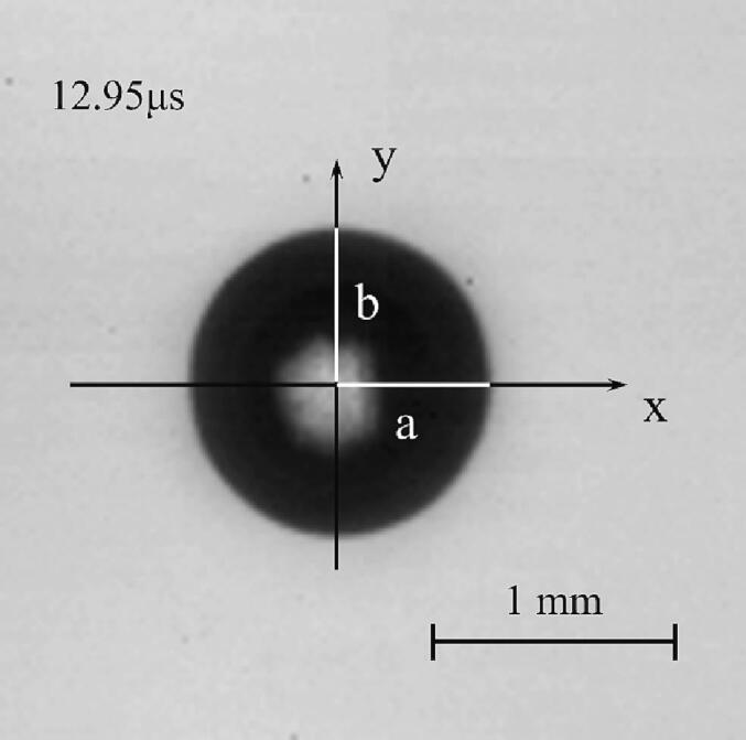
Definition of calculation parameters a and b.

So the equivalent sphere radius is given by

$$R=\sqrt[3]{a{b}^2}$$ (2)

3. Numerical simulation theory

3.1. The extended Gilmore model considering the laser pulse

The Gilmore model [19] is used to calculate the time evolution process of the radius, bubble wall velocity and pressure of cavitation bubble. Gilmore model is proposed based on the dynamics of spherical cavitation bubble. The Gilmore model expression is

$$\left(1-\frac{\dot{R}}{C}\right)R\ddot{R}+\frac{3}{2}\left(1-\frac{\dot{R}}{3C}\right){\dot{R}}^2=\left(1+\frac{\dot{R}}{C}\right)H+\frac{\dot{R}}{C}\left(1-\frac{\dot{R}}{C}\right)R\frac{\mathit{dH}}{\mathit{dR}}$$ (3)

Here, R is the radius of the cavitation bubble, and $\dot{R}$ is the time derivative of the cavitation bubble radius, that is, the velocity of the bubble wall. C and H are respectively expressed as the sound velocity in the liquid at the bubble wall and the enthalpy difference between infinity and the bubble wall. The calculation formula is as follows:

$$C={\left(c_0^2+(n-1)H\right)}^{1/2}$$ (4)

$$H=\frac{n(p_0+B)}{(n-1){\rho }_0}\left[{\left(\frac{P+B}{p_0+B}\right)}^{\frac{n-1}{n}}-1\right]$$ (5)

c₀ is the sound velocity in the liquid under normal conditions, ρ₀ is the density of the liquid, p₀ is the hydrostatic pressure, B and n are determined by experiments, B = 314 MPa and n = 7. For the strong compression of the gas in the bubble when the bubble collapses, the Gilmore model is extended by van der Waals hard core law [15], [30], [31] to account for the volume of non-condensable gas in the bubble. The pressure P at the bubble wall is described by

$$P=\left(p_0+\frac{2\sigma }{R_n}\right){\left(\frac{R_n^3-b{R}_n^3}{R^3-b{R}_n^3}\right)}^{\kappa }-\frac{2\sigma }{R}-\frac{4\mu }{R}\dot{R}$$ (6)

The van der Waals constant is set to b = 1/9 and mainly used to calculate the collapse of the bubble. When the bubble expands, b = 0. κ is the ratio of the specific heat, σ and μ are respectively the surface tension and the dynamic shear viscosity. When the temperature is 20 °C, the values of each parameter are respectively κ = 4/3, σ = 0.072583 N/m and μ = 0.001046 Ns/m³. R_n is the equilibrium radius of the bubble, which means the radius when the internal and external pressures of the bubble are equal, representing the gas content in the bubble. During the laser pulse, the expression of R_n is [21]

$$R_n(t)=\left\{R_0^3+\frac{R_{n1}^3-R_0^3}{2\tau }[t-\frac{\tau }{\pi }\sin \frac{\pi }{\tau }t]\right\}\frac{1}{3}$$ (7)

The laser pulse duration τ = 5 ns. R₀ is the equivalent spherical bubble radius corresponding to the plasma volume after the end of the laser pulse calculated according to photography, and is taken as the initial calculation parameter of the Gilmore model. R_n1 is the equivalent radius when the bubble expands to the maximum radius after a breakdown. And it is the fitting parameter of the model to ensure that the calculated theoretical radius curve is the same as the experimental value.

Eq. (7) describes the gradual deposition of laser energy but does not yet consider the jump-start of the bubble wall velocity originating from the particle velocity in the breakdown shock wave. Neglect of the jump-start leads to an overestimate of the initial bubble pressure and to an underestimation of the initial bubble wall velocity, which affects also the results obtained for shock wave profiles and pressure decay after breakdown as well as for the shock wave energy. Liang et al. [15] updated the approach for modeling laser-induced bubble initiation. Liang et al. [15] rewrote the Gilmore equation such that it describes the evolution of $\ddot{R}$ and add a term ${\dot{u}}_p$ that expresses the evolution of the particle velocity at the bubble wall driven by the energy deposition during the laser pulse. The rewritten equation is as follows:

$$\ddot{R}=-\frac{1}{2}\frac{3C-\dot{R}}{C-\dot{R}}\frac{{\dot{R}}^2}{R}+\frac{C+\dot{R}}{C-\dot{R}}\frac{H}{R}+\frac{\dot{R}}{C}\frac{\mathit{dH}}{\mathit{dR}}+{\dot{u}}_p$$ (8)

During the laser pulse, ${\dot{u}}_p$ is given by the following:

$${\dot{u}}_p=\left({\rho }_0^2{c}_0^2+\frac{4{\rho }_0{c}_2}{\log (10)c_1}P\right)-\frac{1}{2}\frac{2p_0{R}_n(t)+3\sigma }{3R_0^4\tau }\left(R_{n1}^3-R_0^3\right)\left[1-\cos \left(\frac{\pi }{\tau }t\right)\right]$$ (9)

Here, c₁ = 5190 m/s, c₂ = 25306 m/s, P is given by Eq. (6). Only the value of ${\dot{u}}_p$ during the laser pulse (0 ≤ t ≤ 2τ) is determined by Eq. (9), and the other time ${\dot{u}}_p$ = 0.

The expansion of the laser-induced cavitation bubble is mainly driven by the high-temperature water vapor in the bubble. During initial bubble expansion, vapor produced by vaporization of the liquid volume in the plasma condenses. During late expansion, vaporization from the liquid at the bubble wall produces the equilibrium vapor pressure at R_max, and during collapse, vapor condenses again, leading to a smaller R_n at collapse than upon breakdown. In order to characterize this phenomenon, we fit the equilibrium radius in different oscillation periods and adjust the van der Waals radius used to characterize the content of non-condensable gas in the bubble at the same time. As shown in Table 1, t_max1 is the time when the bubble has expanded to the maximum radius, while t_max2 and t_max3 are the times when the bubble have rebounded to the maximum radius after the first and the second collapse, respectively. The change of gas content in the bubble is modeled by changing the value of the equilibrium radius at the maximum radius.

Table 1.

Value of equilibrium radius in different periods.

Time	0-2τ	2τ-tmax1	tmax1-tmax2	tmax2-tmax3	tmax3-tend
Equilibrium radius	Rn(t)	Rn1	Rn2	Rn3	Rn4
van der Waals radius	0	0	bRn2	bRn3	bRn4

3.2. The determination of shock wave emission based on the Kirkwood–Bethe hypothesis

By substituting the cavitation bubble radius, velocity and pressure at the bubble wall calculated by the extended Gilmore model into Kirkwood-Bethe hypothesis, the velocity and pressure distribution of the flow field around the bubble can be calculated, and the location of the shock wave can be determined. Kirkwood-Bethe hypothesis indicates that the invariant quantity G, which propagates along the characteristic line at the velocity of c + u from the bubble wall, is expressed as [25]

$$G=r\left(h+\frac{u^2}{2}\right)=R\left(H+\frac{{\dot{R}}^2}{2}\right)$$ (10)

r is the distance from a point in the flow field to the breakdown center, h is the enthalpy difference between the liquid pressure p and hydrostatic pressure p₀, u is the local liquid velocity, and c is the sound velocity in the liquid. At the bubble wall, r, h and u are replaced by R, H and $\dot{R}$ of the cavitation bubble. The velocity distribution of liquid around the cavitation bubble is given by

$$\frac{\mathit{du}}{\mathit{dt}}=\frac{1}{c-\dot{R}}\left[\left(c+\dot{R}\right)\frac{G}{R^2}-\frac{2c^2\dot{R}}{R}\right],\frac{\mathit{dr}}{\mathit{dt}}=c+\dot{R}$$ (11)

c is given by

$$c=c_0{\left(\frac{p+B}{p_0+B}\right)}^{\frac{n-1}{2n}}$$ (12)

p is the pressure at R

$$p=\left(p_0+B\right){\left[\left(\frac{G}{R}-\frac{{\dot{R}}^2}{2}\right)\frac{\left(n-1\right){\rho }_0}{n\left(p_0+B\right)}+1\right]}^{\frac{n}{n-1}}-B$$ (13)

The velocity and pressure distributions of the flow field around the bubble at a certain time are obtained by taking the bubble radius and the bubble wall velocity as the initial calculation conditions. Several groups of initial conditions at different times are calculated, and multiple characteristic lines are combined to form a network of u (r,t) and p(r,t). By extracting all the points in the network at the same time, we can get the u(r) and p(r) distribution at a certain time, and then the location of the shock front is determined.

To illustrate the method of determining shock wave emission based on Kirkwood-Bethe hypothesis, we use the calculation data in Section 4.2 as an example (Fig. 3 and Fig. 4). The red dotted line in Fig. 3 represents the u(r) data at the bubble wall, and the thin solid lines are the flow field characteristic lines starting from the radius and velocity of the bubble wall at a specific time (0–20 ns). By connecting all the characteristic points at t = 20 ns, the velocity distribution of the flow field around the cavitation bubble at this time is obtained.

Fig. 3.

Distribution of characteristic lines in the flow field from model leading to the u(r) profile at t = 20 ns.

Fig. 4.

Determination of shock front after (a) breakdown and (b) collapse from model.

Fig. 4 (a) and (b) represent the velocity distribution curves in the flow field at specific times after optical breakdown and bubble collapse (T_coll1 = 222.31 μs). The multivalued results given by the curve have no meaning, and only indicate the existence of discontinuity. Following Liang et al. [15], the equal area method is used to determine the location of the shock front. When the enclosed areas on the left and right sides of the vertical line are equal, the position of the vertical line is the position of the shock front. Subsequently, the vertical line is used to replace the curve at the multi-value results on u(r) to indicate the location of the shock front.

3.3. The calculations of bubble and shock wave energies

The final collapse of the cavitation bubble is very fast, and the existing experimental equipment cannot accurately capture the collapse process. However, cavitation bubble expansion and shock wave emission after laser-induced breakdown is very similar to respective processes after collapse, and the initial breakdown condition can be experimentally well controlled. Therefore, the research on collapse shock wave is often replaced by studying the laser-induced shock wave. However, details of both processes may differ and it is, thus, very important to study the energy partition of shock wave and bubble at both breakdown and collapse.

The energy entering the bubble at the breakdown and the energy entering the rebound bubble at the collapse are expressed by calculating the potential energy of the bubble [23], [32]

$$E_{b1}=\frac{4}{3}\pi R_{\max 1}^3\left(p_0-p_v\right)$$ (14)

R_max1 is the maximum radius of the bubble after the breakdown. At 20 °C, the vapor pressure in the bubble p_v = 2330 Pa. The energy E_b2 and E_b3 of the rebound bubble after the first and second collapse are also calculated by Eq. (14) using the respective values of R_maxi.

For the calculation of shock wave energy, it is assumed that the energy dissipated by the shock wave at a point outside the fluid surface is equal to the work done by the shock wave to displace the surface. Assuming that the shock wave is spherically symmetric, the work W_r of the shock wave on the surface with radius r is given by [25]

$$W_r=\int 4\pi r^{2}p(t)udt$$ (15)

where p(t) is the pressure of the shock front, u is the particle velocity for the shell of radius r and udt is its displacement in time dt. u is given by

$$u=\frac{p(t)-p_0}{{\rho }_0{c}_0}$$ (16)

Eq. (16) is the first order approximation derived by Gilmore [19]. Ignoring the hydrostatic pressure p₀, and substituting Eq. (16) into Eq. (15), we obtain the shock wave energy at a fixed position

$$E_s=\frac{4\pi r2}{\rho 0c0}\int p{(t)}^{2}dt$$ (17)

Using to the shock wave pressure p(t) calculated by the extended Gilmore model and Kirkwood-Bethe hypothesis, the shock wave energy can be obtained by integrating all the shock front pressures at a fixed distance r = 6 R₀ within a time interval that starts, when the shock front has propagated to this position and ends, when the bubble wall has reached it. At this time, the shock wave has a steep rising edge and an exponentially decaying falling edge. Moreover, r is then far greater than the thickness of the shock wave and we can use a fixed value of r in Eq. (17) for calculating E_6R0. For the calculation of shock wave energy after at the first and second bubble collapses, the integration positions are r = 6 R_min1 and r = 6 R_min2 respectively. R_min1 and R_min2 are the minimum radii of the first and second collapses respectively.

However, the approach of calculating shock wave energy through Eq. (17) underestimates the total shock wave energy because the large amount of energy dissipated during propagation up to r = 6 R₀ is not accounted for. Therefore, Vogel et al. [27] presented another approach, where the shock wave energy is determined by integrating the dissipation losses in the near field based on measured shock wave propagation data and adding the shock wave energy in the far field obtained from hydrophone measurements. The dissipated shock wave energy E_diss during propagation up to r = 6 R₀ is given by [27]

$$E_{\mathit{diss}}={\int }_{r0}^{r1}4\pi r^2{\rho }_s(r)\mathrm{\Delta }\epsilon (r)dr$$ (18)

Eq. (18) represents the internal energy change during the propagation of a spherical shock front from r₀ to r₁. Δε(r) is given by

$$\mathrm{\Delta }\epsilon (r)=\frac{1}{2}\left(\frac{1}{{\rho }_0}-\frac{1}{{\rho }_s(r)}\right)p_s(r)$$ (19)

Here, ρ_s is the shock wave density and p_s is the shock wave pressure. ρ_s is given by

$${\rho }_s=\frac{\rho 0}{1-\frac{\mathit{Ps}}{u_s^2\rho 0}}$$ (20)

u_s is the shock wave velocity. u_s(r) and p_s(r) are calculated based on the Kirkwood-Bethe hypothesis.

In addition, it is also necessary to consider the energy needed for vaporization of the liquid in the plasma volume for establishing an energy balance of optical breakdown [15], [27]. To assess the evaporation energy, Vogel et al. [27] assumed that the water within the plasma volume is completely evaporated, but neglected any enlargement of the evaporated liquid volume by heat conduction. During optical breakdown, the energy E_v needed for vaporization of the liquid in the plasma volume V_p is given by

$$E_v={\rho }_0{V}_p\left[C_p\left(T_2-T_1\right)+L_v\right]$$ (21)

Here, V_p = (4/3)πR₀³, C_p = 4187 J/(K kg), L_v = 2256 kJ/kg, T₁ = 20 °C, and T₂ = 100 °C.

4. Results and discussions

4.1. Dynamics of the spherical cavitation bubble

A total of five groups of experiments were conducted under the same experimental conditions, and one R(t) curve was deduced from the combined results of all experiments. This was possible because of the high reproducibility of laser-induced bubble formation in our experiments. The deviations of the maximum radii after the optical breakdown, the first collapse and the second collapse were calculated to be 1208 μm ± 5 μm, 465 μm ± 14 μm and 275 μm ± 10 μm, respectively. Fig. 5 shows the evolution process of cavitation bubble oscillation in four cycles captured by high-speed camera. The cavitation bubble remains highly spherical most of the time before 301 μs and is non-spherical only for a short time after breakdown and collapse. The time interval between two images taken by high-speed camera is relatively long (1.295 μs), the initial plasma and shock wave at the breakdown and the bubble collapse are not captured.

Fig. 5.

Time evolution sequence of cavitation bubble.

In order to assess whether the millimeter cavitation bubble captured in the experiment can be considered as a spherical cavitation bubble, the sphericity of the bubble needs to be evaluated. In addition to the slender plasma produced during the optical breakdown, the hydrostatic pressure difference between the upper and lower bubble walls of the cavitation bubble will also affect the sphericity of the bubble. When the hydrostatic pressure difference is large enough, it will lead to upward movement in the process of oscillation, and a liquid jet will form through the entire bubble when it collapses because of the conservation of Kelvin impulse [33]. Therefore, it is also necessary to evaluate the impact of buoyancy on the bubble. The influence of buoyancy [34] can be evaluated by

$$\delta ={\left(\frac{{\rho }_{0}g{R}_{\max 1}}{p_0-p_v}\right)}^{1/2}$$ (22)

ρ₀ is the density of water, g is the acceleration of gravity, and R_max1 is the maximum radius of the bubble, where R_max1 = 1.205 mm, p₀ and p_v are hydrostatic pressure and saturated vapor pressure respectively. By calculation, δ = 0.01.

When the buoyancy and the force acting from an adjacent rigid wall surface on the cavitation bubble are in balance over a pulsation, the resulting Kelvin impulse is zero. The dimensionless stand-off distance γ is defined as γ = d / R_max1, where d is the distance from the center of mass of the bubble to the wall surface. For zero Kelvin impulse, the following relationship between the buoyancy parameters δ and γ holds [34], [35]:

$$\delta ·\gamma =0.442$$ (23)

If δγ > 0.442, the bubble will migrate away from the boundary, while for δγ < 0.442, the bubble will migrate toward the boundary [34], [35]. We can also use Eq. (23) to estimate the influence of buoyancy on the bubble. When δ = 0.01, buoyancy must be counteracted by a wall influence corresponding to γ = 44.2 to yield zero Kelvin impulse. The large γ value indicates that the influence of buoyancy on the bubble is very small.

To further support this finding, we used the boundary integral method developed by Blake et al. [36] and Supponen et al. [37] to simulate the expansion and collapse process of the cavitation bubble with a maximum radius of 1.2 mm under the gravity gradient. This method assumes that the fluid is incompressible, inviscid and irrotational, and ignores the surface tension. Fig. 6 shows the process of bubble expansion (gray line) and collapse (black line) obtained by the simulation, and there is no micro-jet during the collapse. Even if a micro-jet is generated during bubble collapse, it is very weak and its energy is almost negligible. Therefore, we think that the cavitation bubble can be treated as a spherical bubble. It should be mentioned that Obreschkow et al. [13] observed a pronounced jet for bubbles with R_max = 4 mm, which is not so much larger than R_max = 1.2 mm.

Fig. 6.

Time evolution of cavitation bubble expansion (gray line) and collapse (black line) from model.

The initial radius R₀ and bubble wall velocity U₀ are substituted into the extended Gilmore model, and the curves of bubble radius, velocity and pressure with respect to time are obtained. In order to determine the initial input parameters of the extended Gilmore model, it is also necessary to determine the initial plasma size. Therefore, we used a time gated ICCD camera (Andor Technology, iStar DH 734i) to capture the plasma formation process, while ensuring that the energy of the laser pulse and the experimental environment remain unchanged. The exposure time of the photographs is 2 ns. As shown in Fig. 7, the plasma is completely deposited at 10 ns. A brighter core located within the laser cone angle is surrounded by a diffusely luminescent region that likely arises from radiative energy transport [38]. We ignore the diffuse halo around the plasma core and determine the initial equivalent spherical radius R₀ is obtained by calculating the volume of the plasma core. This way, R₀ is calculated to be about 19 μm.

Fig. 7.

Process of laser pulse plasma deposition.

The detailed cavitation bubble collapse process was not captured through experiments, but we can try to restore the collapse process through calculation. Table 2 shows the input parameters and calculation results of the extended Gilmore model. Fig. 8 shows the comparison between the bubble radius obtained by the extended Gilmore model and the experimental data, and the time evolution of bubble wall velocity and pressure in bubble. The four colors in Fig. 8 represent the first four periods of cavitation bubble oscillation respectively. As shown in Fig. 8 (a), the red dotted line shows the value change of the equilibrium radius R_n, and the green dotted line shows the value change of bR_n. By changing the value of R_n, excellent agreement between the calculation results of the extended Gilmore model and the radius measured in the experiment could be achieved for the first four bubble oscillation cycles. This indicates that for the millimeter-scale cavitation bubble, the fourth oscillation is still inertially governed and the water vapor in the bubble is almost completely condensed at this stage. Condensation and vaporization play little role for the shape of the R(t) curve. In comparison, Zhong et al. [39] used a complex model to consider thermal condensation, evaporation and conduction at the thermal boundary layers with four free-fitting parameters to model the dynamics of a laser-induced bubble that was not perfectly spherical. Experimental R(t) data for the bubble with R_max ∼ 1.1 μm could be fitted well only for the first two oscillations. By contrast, for highly spherical bubbles as used in the present study using a single parameter R_n is sufficient to simulate condensation at the bubble wall.

Table 2.

Input parameters and calculation results of extended Gilmore model.

Instant	Time (μs)	R (μm)	Rn (μm)	bRn (μm)
R0	0	19	424.5	0
Rmax1	111.44	1207.56	–	–
1st collapse	222.31	22.12	186	20.67
Rmax2	266.67	477.05	–	–
2nd collapse	310.53	14.09	108	12
Rmax3	336.00	273.82	–	–
3rd collapse	361.30	12.80	82.5	9.17
Rmax4	380.13	201.75	–	–
4th collapse	399.18	19.22	82.5	9.17

Fig. 8.

Time evolution of (a) bubble radius, (b) bubble wall velocity and (c) internal pressure in the whole oscillation process. The red dots in (a) are from experiment, and the black solid lines in (a), (b) and (c) are from model. (For interpretation of the references to colour in this figure legend, the reader is referred to the web version of this article.)

The bubble starts to expand from R₀ = 19 μm. The constant increase of R_n simulates the continuous deposition of energy during the laser pulse. Compared with the femtosecond laser pulse used by Liang et al. [15], the optical breakdown process of the nanosecond laser pulse is more intense and the bubble wall velocity and pressure in the bubble are greater. During the breakdown process, the calculated peak velocity of the bubble wall is 2700 m/s, and the pressure in the bubble is 5.65 GPa. The bubble wall velocity is slightly larger than the experimental value of 2500 m/s determined by Vogel et al. for a 10-mJ, 6-ns laser pulse [21]. Subsequently, the bubble continues to expand, and the velocity and pressure continue to decrease. When the bubble collapses, the bubble will rebound when it shrinks to a certain size due to the influence of the mixture of vapor and permanent gas in the bubble. The minimum radius of the bubble at the first collapse is 22.12 μm, and the bubble wall velocity and pressure are 1088 m/s and 4.77 GPa respectively, which are lower than those at the breakdown. With the continuous decrease of the gas content in the bubble, the pressure and velocity at the bubble collapse decrease until the bubble disappears.

4.2. Simulation of shock wave emission

Fig. 9 shows the time evolution of the velocity and pressure distribution in the flow field around the cavitation bubble after the optical breakdown, the first collapse and the second collapse. Fig. 9 (a) and (b) shows the evolution of velocity distribution and pressure distribution in the flow field within 5–600 ns after the breakdown. The black dot at the beginning of each curve represents the position and velocity of the bubble wall at that time; the blue dot in Fig. 9 (b) represents the position and pressure of the shock front at that time, and the blue dotted line represents the pressure attenuation of the shock front. The shock front begins to form at 5 ns, and then the pressure of the shock wave starts to decrease after a short rise, similar to the results of Vogel et al. [21] and Lai et al. [26]. The attenuation of shock wave pressure is mainly divided into three characteristic stages. First, the slope of the p(r) curve is about −1, then it decreases to −2, and finally it is less than −2.

Fig. 9.

Simulated velocity and pressure distribution in flow field after the breakdown, the first collapse and the second collapse from model. (a) and (b) for the breakdown, (c) and (d) for the first collapse, (e) and (f) for the second collapse.

By considering the condensation of water vapor in the bubble in the process of bubble oscillation through changing the value of R_n, the whole oscillation process of the spherical bubble can be accurately simulated, which also provides a new basis for calculating the velocity, pressure distribution, and energy of collapse shock wave. We calculate the evolution of velocity distribution and pressure distribution in the flow field after the first collapse (Fig. 9 (c) and (d)) and the second collapse (Fig. 9 (e) and (f)), respectively, starting from the time of the first collapse (T_coll1 = 222.31 μs) and the second collapse (T_coll2 = 310.53 μs).

The red dotted line and the black solid line in Fig. 9 (c) and (d) are the velocity and pressure distributions in the flow field at a specific time before and after the collapse, respectively. The shock front starts to form 8 ns after the collapse. Compared with the shock wave at the breakdown, the shock wave at the first collapse has lower pressure and slower energy attenuation. In the study of shock wave emission of micron-sized spherical cavitation bubbles given by Liang et al. [15], the collapse shock wave pressure is higher than the breakdown shock wave pressure. Liang et al. [15] have already given an explanation: low plasma energy density and temperature at breakdown produces little permanent gas through water dissociation, which can later buffer the collapse. Therefore, the collapse pressure is high. In the present study, the plasma energy density is obviously high, which leads to intense gas production at breakdown and a less vigorous collapse with comparatively large rebound bubble. This, in turn, results in a strong second collapse still accompanied by weak shock wave emission, which is not always observed in laser-induced cavitation. Plasma energy density does not only affect peak pressure but also energy partitioning into shock wave and bubble energy.

Liang et al. [15] who first pointed this out that before the bubble collapses, the pressure in the liquid around the bubble is much higher than the pressure at the bubble wall. As a result, the liquid around the bubble is compressed in the process of bubble contraction, and part of the energy is stored in the compressed liquid around the bubble. It was demonstrated by Liang et al. [15] that the energy of the shock wave at bubble collapse comes not only from the internal energy of the bubble but also from the compression energy in the liquid, and the energy in the compressed liquid is far greater than that in the bubble. Our results are the same as those of Liang et al. [15]. This shows that the formation mechanism of shock wave at bubble collapse is different from that at the optical breakdown. The shock wave after breakdown is driven by the high-temperature and high-pressure vapor in the bubble, while the shock wave after the collapse is mainly driven by the compressed liquid around the bubble and only partly by the compressed vapor and gas within the bubble.

Fig. 9 (e) and (f) show the evolution of velocity distribution and pressure distribution in the flow field after the second bubble collapse. At this time, the internal energy of the bubble and the compression energy in the liquid are very small, and the intensity of the shock wave generated is much weaker than that after the first collapse. The wave front of the shock wave starts to form 30 ns after the second collapse.

4.3. Energy partition up to the fourth oscillation

For calculating the shock wave energy, it is necessary to know the shock wave width δ_sw and the shock wave duration τ_sw. Fig. 10 shows the definition of shock wave width δ_sw at the optical breakdown and bubble collapses. For the breakdown shock wave, the distance between half of the shock front pressure and the left intersection point of the curve with the trailing edge of the shock wave is the shock wave width δ_sw. For the collapse shock wave, the distance between half of the pressure rise at the shock front and the left intersection of the curve with the wave is the width of the shock wave δ_sw. The ratio of shock wave width and velocity at this moment yields the shock wave duration τ_sw = δ_sw / u_sw.

Fig. 10.

Determination of shock wave width δ_sw at the breakdown (a) and bubble collapse (b) from model.

Fig. 11 shows the integral interval of the shock wave pressure at a fixed position when calculating the energy of the breakdown shock wave. The integration starts at the time t₀ = 35 ns, when the shock front has propagated to the integration position (r = 6 R₀) and ends at the time t_end = 171 ns, when the bubble wall has reached this position. The shock wave energy is then calculated by Eq. (17).

Fig. 11.

The integration interval for calculating the energy of the breakdown shock wave.

The energy E_b entering the cavitation bubble and the shock wave energy E_6R0 at r = 6 R₀ are calculated using Eq. (14) and Eq. (17) respectively. Table 3 compares the calculation results obtained by integration over shock wave profiles at r = 6 R₀ with those obtained by Vogel et al. [21] and Lai et al. [26]. The shock wave width δ_sw and duration τ_sw are calculated when the shock front has propagated to 6 R₀. The data in columns 2 to 5 in Table 3 were calculated using the traditional Gilmore model [19], and the data in column 6 were calculated using the extended Gilmore model by Liang et al. [15]. The data in column 5 and 6 are from the same set of experimental data, and the difference is that different models are used. The results show that the ratio of E_6R0 and E_b at the breakdown is 0.79:1, and the ratio of shock wave width δ_sw to initial radius R₀ is 1.98:1 by using the extended Gilmore model, which differs considerably from the results of Vogel et al. [21] and Lai et al. [26] obtained by using the traditional Gilmore model. Consideration of the jump-start of the bubble wall velocity originating from the particle velocity in the breakdown shock wave yields smaller values of the calculated shock wave pressure and shock wave energy. The vaporization energy E_v during breakdown is 74.27 μJ. Its energy fraction is very small, in agreement with the result of Vogel et al. [27].

Table 3.

Energy partition at the optical breakdown.

Laser parameter	6 ns–10 mJ [21]	12 ns–22 mJ [26]	12 ns–45 mJ [26]	5 ns–10 mJ	5 ns–10 mJ
Adopted model	Gilmore model	Gilmore model	Gilmore model	Gilmore model	Extended Gilmore model
Initial bubble radius R0 (μm)	37	10.4	15.2	19	19
Maximum bubble radius Rmax (μm)	1820	1075.3	1439.9	1206.4	1207.56
Bubble energy Eb (μJ)	2500	508.7	1221.5	718.33	720.40
Shock wave width δsw (μm)	114	29.3	46.3	54.4	37.7
Normalized shock wave width δsw/R0	3.1	2.82	3.04	2.87	1.98
Local shock wave velocity usw (m/s)	2053	2713.1	2778.3	2290.2	2188
shock wave duration τsw (ns)	58	10.8	16.7	24.2	17.23
Shock wave energy E6R0 at r = 6R0 (μJ)	4190	1158.2	2911.0	1476.9	568.33
The ratio of the shock wave energy to bubble energy E6R0/Eb	1.68	2.28	2.38	2.06	0.79

Table 4 shows the calculation results for shock wave energy E_sw = E_diss + E_6R0 and cavitation bubble energy E_b at the breakdown, at the first collapse and the second collapse. The values for the breakdown shock wave energy and for E_sw / E_b are much larger than the respective values in the last column of Table 3, where only E_6R0 was considered. During the oscillations of the cavitation bubble, the bubble energy and shock wave energy decrease continuously. At the second collapse, the energy of the shock wave and the bubble is already very small. The velocity u_sw, width δ_sw and duration τ_sw of the shock wave at the positions r = 6 R_min1 and or r = 6 R_min2 are also gradually reduced.

Table 4.

Energy partition at the optical breakdown, 1st collapse and 2nd collapse.

Instant	At breakdown	1st collapse	2nd collapse
Initial bubble radius R0 or Rmin (μm)	19	22.12	14.09
Maximum bubble radius Rmax (μm)	1207.56	477.05	273.82
Bubble energy Eb (μJ)	720.40	44.42	8.40
Shock wave width δsw (μm)	37.7	25.92	19.99
Normalized shock wave width δsw/R0 or δsw/Rmin	1.98	1.17	1.42
Local shock wave velocity usw (m/s)	2188	2053	1787
shock wave duration τsw (ns)	17.23	12.63	11.19
Shock wave energy E6R0 at r = 6R0 or r = 6Rmin (μJ)	568.33	333.43	21.36
Dissipated energy Ediss (μJ)	611.21	312.50	2.22
Shock wave energy Esw = E6R0 + Ediss (μJ)	1179.54	645.93	23.58
The ratio of the shock wave energy to bubble energy Esw/Eb	1.64	14.54	2.81

By considering also the energy dissipated during propagation up to r = 6 R₀, we obtain the total energy of the shock wave E_sw = E_diss + E_6R0. The results show that the ratio E_sw / E_b after breakdown is 1.64:1. Compared to previous studies, our results are similar to those of Teslenko [22] and Vogel et al. [27] (about 2:1), but larger than those of Vogel et al. [23] and Liang et al. [15] (about 0.7:1). We believe that the reasons for the difference are: 1) Plasma energy density is different; 2) The methods for calculating shock wave energy are different.

The potential energy E_b1 of the bubble when the bubble has expanded to the maximum radius after the optical breakdown is taken as the total energy at the first collapse. About 89.7% of that energy is consumed by the shock wave emission, only about 6.2% of the energy enters the rebound bubble, and about 4.1% fraction of energy lost by condensation and viscous damping is estimated by subtracting (E_diss + E_6R0 + E_b) from 100%. The rebound bubble energy is relatively high in the present paper (6.2% of the bubble energy compared to 3.0% in Liang et al. [15]), which indicates a relatively large permanent gas content of the collapsing bubble that buffered the collapse and reduced shock wave pressure. This is consistent with a large plasma energy density. The ratio of shock wave energy to rebound bubble energy is about 14.54:1.

At the second collapse of the bubble, the energy partition is different from the first collapse, about 53.1% of the energy is consumed by the emission of the shock wave, and about 18.9% of the energy enters the bubble. The ratio of shock wave energy to rebound bubble energy is about 2.81:1. The ratio of the shock wave width to the minimum radius is 1.17:1 at the first collapse and 1.42:1 at the second collapse.

The shock wave energy at the third and fourth collapse, its energy is very small. When we use the Kirkwood–Bethe hypothesis to calculate the pressure profile of the shock wave at the third and fourth collapse, we find that no shock front evolves. Therefore, we cannot directly calculate the shock wave energy. However, we can estimate the maximum shock wave energy by comparing the bubble energy before collapse with the rebound bubble energy after collapse using Eq. (14). R_max5 = 179.60 µm is calculated by the extended Gilmore model. The bubble energy before the third collapse is 8.4 µJ (Table 3), and the rebound bubble energies after the third and fourth collapse are 3.36 μJ and 2.37 μJ, respectively. The estimate indicates that the shock wave energies of the third and fourth collapses are not higher than 5.04 μJ and 0.99 μJ, respectively. The ratio of shock wave energy to bubble energy at the third and fourth collapse is less than 1.5 and 0.42. It can be seen that after the first collapse, the ratio of the collapse shock wave energy to bubble energy becomes smaller and smaller.

In this paper, we explored in detail the energy partitioning between the shock wave and the cavitation bubble from optical breakdown up to the fourth oscillation. We investigated the different formation mechanisms of the breakdown shock wave and collapse shock wave, which is relevant for understanding the mechanism of cavitation erosion. Because it is very challenging to record the shock wave propagation after collapse, it is difficult to measure the energy of each part after collapse by experiment. Therefore, the accuracy of our simulation results still remains to be experimentally verified. In addition, the energy dissipation in the process of cavitation bubble oscillation and the energy partitioning for aspherical collapse with micro-jet formation need to be further researched.

5. Conclusions

A millimeter-scale spherical cavitation bubble produced by a nanosecond laser pulse was experimentally studied using a high-speed camera, and the oscillation process of the cavitation bubble was simulated based on the extended Gilmore model and Kirkwood-Bethe hypothesis. The shock wave emission and shock front pressure attenuation processes was simulated up to the fourth oscillation, and the energy partitioning for the millimeter-scale cavitation bubble was successfully calculated. The main conclusions are as follows:

• (1)If the continuous condensation of vapor in the bubble during the oscillations of the bubble is considered by a stepwise reduction of equilibrium radius R_n, the time evolution of bubble radius, bubble wall velocity and bubble pressure in the first four oscillation cycles can be calculated very accurately. When the bubble collapses for the first time, the bubble wall velocity reached 1088 m/s, and the bubble’s internal pressure reached 4.77 GPa.
• (2)The time evolution of shock wave velocity and pressure at the optical breakdown and the first and second collapse of the bubble were calculated. The peak pressure was found to be largest for the shock wave generated by the optical breakdown.
• (3)The energy of the shock wave and the energy entering the bubble were calculated up to the fourth oscillation. The ratio of shock wave energy to bubble energy at the optical breakdown, first collapse and second collapse was 1.64, 14.54 and 2.81 respectively, and the ratio of shock wave energy to bubble energy at the third collapse is less than 1.5. A large part of the energy of the shock wave emitted during collapse comes from the compressed liquid around the bubble.

Declaration of Competing Interest

The authors declare that they have no known competing financial interests or personal relationships that could have appeared to influence the work reported in this paper.

References

- 1.Vogel A., Schweiger P., Frieser A., Asiyo M.N., Birngruber R. Intraocular Nd: YAG laser surgery: laser-tissue interaction, damage range, and reduction of collateral effects. IEEE J. Quantum Electron. 1990;26:2240–2260. [Google Scholar]
- 2.Ozkurt Y.B., Sengör T., Evciman T., Haboğlu M. Refraction, intraocular pressure and anterior chamber depth changes after Nd: YAG laser treatment for posterior capsular opacification in pseudophakic eyes. Clin. Exp. Optom. 2009;92:412–415. doi: 10.1111/j.1444-0938.2009.00401.x. [DOI] [PubMed] [Google Scholar]
- 3.Dretler S.P. Laser lithotripsy: a review of 20 years of research and clinical applications. Lasers Surg. Med. 1988;8:341–356. doi: 10.1002/lsm.1900080403. [DOI] [PubMed] [Google Scholar]
- 4.Albu C., Dinescu A., Filipescu M., Ulmeanu M., Zamfirescu M. Periodical structures induced by femtosecond laser on metals in air and liquid environments. Appl. Surf. Sci. 2013;278:347–351. [Google Scholar]
- 5.A.H. Hamad, K.S. Khashan, A.A. Hadi, Laser Ablation in Different Environments and Generation of Nanoparticles, Applications of Laser Ablation – Thin Film Deposition, Nanomaterial Synthesis and Surface Modification, (2016) 177–196.
- 6.Philipp A., Lauterborn W. Cavitation erosion by single laser-produced bubbles. J. Fluid Mech. 1998;361:75–116. [Google Scholar]
- 7.Fujisawa N., Fujita Y., Yanagisawa K., Fujisawa K., Yamagata T. Simultaneous observation of cavitation collapse and shock wave formation in cavitating jet. Exp. Therm Fluid Sci. 2018;94:159–167. [Google Scholar]
- 8.Zhang S., Yao Z., Wu H., Zhong Q., Tao R., Wang F. A New Turbulent Viscosity Correction Model With URANS Solver for Unsteady Turbulent Cavitation Flow Computations. J. Fluids Eng. 2022;144 [Google Scholar]
- 9.Lauterborn W., Bolle H. Experimental investigations of cavitation-bubble collapse in the neighbourhood of a solid boundary. J. Fluid Mech. 1975;72:391–399. [Google Scholar]
- 10.Wang S.-P., Zhang A.M., Liu Y.-L., Zhang S., Cui P. Bubble dynamics and its applications. J. Hydrodyn. 2018;30:975–991. [Google Scholar]
- 11.Ohl C.D., Philipp A., Lauterborn W. Cavitation bubble collapse studied at 20 million frames per second. Annalen der Physik. 1995;507:26–34. [Google Scholar]
- 12.Tinguely M., Ohtani K., Farhat M., Sato T. Observation of the Formation of Multiple Shock Waves at the Collapse of Cavitation Bubbles for Improvement of Energy Convergence. Energies. 2022;15:2305. [Google Scholar]
- 13.Obreschkow D., Tinguely M., Dorsaz N., Kobel P., De Bosset A., Farhat M. Universal scaling law for jets of collapsing bubbles. Phys. Rev. Lett. 2011;107 doi: 10.1103/PhysRevLett.107.204501. [DOI] [PubMed] [Google Scholar]
- 14.Obreschkow D., Tinguely M., Dorsaz N., Kobel P., De Bosset A., Farhat M. The quest for the most spherical bubble: experimental setup and data overview. Exp. Fluids. 2013;54:1–18. [Google Scholar]
- 15.Liang X.-X., Linz N., Freidank S., Paltauf G., Vogel A. Comprehensive analysis of spherical bubble oscillations and shock wave emission in laser-induced cavitation. J. Fluid Mech. 2022;940:A5. [Google Scholar]
- 16.Rayleigh L. Viii. On the pressure developed in a liquid during the collapse of a spherical cavity. The London, Edinburgh, and Dublin Philos. Mag. J. Sci. 1917;34:94–98. [Google Scholar]
- 17.M.S. Plesset, The dynamics of cavitation bubbles, (1949).
- 18.Herring C. Diffusional viscosity of a polycrystalline solid. J. Appl. Phys. 1950;21:437–445. [Google Scholar]
- 19.F.R. Gilmore, The growth or collapse of a spherical bubble in a viscous compressible liquid, (1952).
- 20.Keller J.B., Miksis M. Bubble oscillations of large amplitude. J. Acoust. Soc. Am. 1980;68:628–633. [Google Scholar]
- 21.Vogel A., Busch S., Parlitz U. Shock wave emission and cavitation bubble generation by picosecond and nanosecond optical breakdown in water. J. Acoust. Soc. Am. 1996;100:148–165. [Google Scholar]
- 22.Teslenko V. Investigation of photoacoustic and photohydrodynamic parameters of laser breakdown in liquids. Sov. J. Quantum Electron. 1977;7:981. [Google Scholar]
- 23.Vogel A., Lauterborn W. Acoustic transient generation by laser-produced cavitation bubbles near solid boundaries. J. Acoust. Soc. Am. 1988;84:719–731. [Google Scholar]
- 24.Vogel A., Lauterborn W., Timm R. Optical and acoustic investigations of the dynamics of laser-produced cavitation bubbles near a solid boundary. J. Fluid Mech. 1989;206:299–338. [Google Scholar]
- 25.Cole R.H., Weller R. Underwater explosions. Phys. Today. 1948;1:35. [Google Scholar]
- 26.Lai G., Geng S., Zheng H., Yao Z., Zhong Q., Wang F. Early dynamics of a laser-induced underwater shock wave. J. Fluids Eng. 2022;144 [Google Scholar]
- 27.Vogel A., Noack J., Nahen K., Theisen D., Busch S., Parlitz U., Hammer D., Noojin G., Rockwell B., Birngruber R. Energy balance of optical breakdown in water at nanosecond to femtosecond time scales. Appl. Phys. B Lasers Opt. 1999;68 [Google Scholar]
- 28.Tinguely M., Obreschkow D., Kobel P., Dorsaz N., De Bosset A., Farhat M. Energy partition at the collapse of spherical cavitation bubbles. Phys. Rev. E. 2012;86 doi: 10.1103/PhysRevE.86.046315. [DOI] [PubMed] [Google Scholar]
- 29.Hickling R., Plesset M.S. Collapse and rebound of a spherical bubble in water. Phys. Fluids. 1964;7:7–14. [Google Scholar]
- 30.Löfstedt R., Barber B.P., Putterman S.J. Toward a hydrodynamic theory of sonoluminescence. Phys. Fluids A Fluid Dyn. 1993;5:2911–2928. [Google Scholar]
- 31.Lauterborn W., Kurz T. Physics of bubble oscillations. Rep. Prog. Phys. 2010;73 [Google Scholar]
- 32.Brennen C.E. Cambridge University Press; 2014. Cavitation and bubble dynamics. [Google Scholar]
- 33.Benjamin T.B., Ellis A.T. The collapse of cavitation bubbles and the pressures thereby produced against solid boundaries. Philos. Trans. R. Soc. London. Ser. A. 1966:221–240. [Google Scholar]
- 34.Blake J., Taib B., Doherty G. Transient cavities near boundaries. Part 1. Rigid boundary. J. Fluid Mech. 1986;170:479–497. [Google Scholar]
- 35.Brujan E., Pearson A., Blake J. Pulsating, buoyant bubbles close to a rigid boundary and near the null final Kelvin impulse state. Int. J. Multiph. Flow. 2005;31:302–317. [Google Scholar]
- 36.Blake J.R., Gibson D. Cavitation bubbles near boundaries. Annu. Rev. Fluid Mech. 1987;19:99–123. [Google Scholar]
- 37.Supponen O., Obreschkow D., Kobel P., Tinguely M., Dorsaz N., Farhat M. Shock waves from nonspherical cavitation bubbles. Phys. Rev. Fluids. 2017;2 [Google Scholar]
- 38.Vogel A., Nahen K., Theisen D., Noack J. Plasma formation in water by picosecond and nanosecond Nd: YAG laser pulses. I. Optical breakdown at threshold and superthreshold irradiance. IEEE J. Sel. Top. Quantum Electron. 1996;2:847–860. [Google Scholar]
- 39.Zhong X., Eshraghi J., Vlachos P., Dabiri S., Ardekani A.M. A model for a laser-induced cavitation bubble. Int. J. Multiph. Flow. 2020;132 [Google Scholar]