Human examination and artificial intelligence in cephalometric landmark detection—is AI ready to take over?

Abstract

Objectives:

To compare the precision of two cephalometric landmark identification methods, namely a computer-assisted human examination software and an artificial intelligence program, based on South African data.

Methods:

This retrospective quantitative cross-sectional analytical study utilized a data set consisting of 409 cephalograms obtained from a South African population. 19 landmarks were identified in each of the 409 cephalograms by the primary researcher using the two programs [(409 cephalograms x 19 landmarks) x 2 methods = 15,542 landmarks)]. Each landmark generated two coordinate values (x, y), making a total of 31,084 landmarks. Euclidean distances between corresponding pairs of observations was calculated. Precision was determined by using the standard deviation and standard error of the mean.

Results:

The primary researcher acted as the gold-standard and was calibrated prior to data collection. The inter- and intrareliability tests yielded acceptable results. Variations were present in several landmarks between the two approaches; however, they were statistically insignificant. The computer-assisted examination software was very sensitive to several variables. Several incidental findings were also discovered. Attempts were made to draw valid comparisons and conclusions.

Conclusions:

There was no significant difference between the two programs regarding the precision of landmark detection. The present study provides a basis to: (1) support the use of automatic landmark detection to be within the range of computer-assisted examination software and (2) determine the learning data required to develop AI systems within an African context.

Introduction

Cephalometric landmark detection is important for orthodontic diagnosis and treatment planning. Digital cephalometry is the current gold-standard. The progression to computer-assisted-cephalometric analysis was directed at improving the diagnostic value by reducing random errors and saving time. ¹ Cephalometric landmark detection is generally tedious, time-consuming and prone to subjectivity. The most common cause of random errors, in both manual and computer-aided cephalometry, is inconsistency in landmark detection. As a result, attempts to use artificial intelligence (AI) in cephalometric landmark detection have been made. ^2–5

AI refers to algorithms that perform tasks conventionally associated with human intelligence. ^6–8 Lindner et al ⁵ points out that computerized landmark detection systems can significantly improve the clinical workflow in orthodontic treatment. Lindner et al developed a fully automatic landmark annotation (FALA) system (BoneFinder^®) for identifying cephalometric landmarks. This system was awarded first prize at the 2015 ISBI Grand Challenge in Dental X-ray Image Analysis. Literature states that landmark detection errors of less than 2 mm are clinically acceptable. ^4,9

Hwang et al ¹⁰ compared detection patterns of 80 landmarks identified by an AI system based on You-Only-Look-Once v. 3 with human examination. The human intraexaminer variability of repeated manual detections revealed a detection error of 0.97–1.03 mm. Their AI system consistently detected identical positions, upon repeated trials. Silva et al ¹ also found it to be a promising tool to enhance the linear and angular measurements used in Arnett’s analysis.

Currently, literature regarding the precision and accuracy of automated cephalometric landmark detection is limited within a South African context. Moreover, studies exploring landmark detection amongst mixed ancestry and different racial profiles are sparse. Furthermore, no comparisons have been done comparing the computer-assisted human examination approach using Dolphin Imaging^® and BoneFinder^® regarding cephalometric landmark detection. Therefore, this study aimed to determine the precision of two cephalometric landmark identification methods, namely, a computer-assisted human examination software (Dolphin Imaging^®) and an AI program (BoneFinder^®).

Methods and materials

The Biomedical Science Research Ethics Committee of the University of the Western Cape (UWC) approved the research protocol (BM19/10/3) and it was carried out according to STROBE guidelines.

Sampling

The study population consisted of retrospective cephalograms of patients who required orthodontic treatment and presented at the Radiology Department of the Faculty of Dentistry, Tygerberg Oral Health Center, UWC, South Africa. No cephalograms were specifically taken for the study and no patients were exposed to unnecessary radiation to fulfil sample size requirements.

Inclusion criteria

1. Pre-operative cephalograms of patients requiring orthodontic treatment, but no evidence of orthodontic treatment

2. Patients with no missing permanent incisors or first molars

3. Cephalograms of patients in occlusion

4. Cephalograms of diagnostic quality

5. No unerupted or supernumerary teeth overlying areas of interest

6. Cephalograms with correct cephalostat placement.

Exclusion criteria

1. Peri- and post-operative cephalograms

2. Cephalograms of patients with gross skeletal asymmetries and anomalies

3. Cephalograms with distortion and artifacts superimposed overlying areas of interest

4. Cephalograms without a cephalostat.

Instruments and machines

All cephalograms were acquired in DICOM and JPEG format with the Orthophos XG five machine (Dentsply Sirona, Germany) using Sidexis (v. 4.3). The image resolution was 1280 × 1024 pixels. The cephalograms were taken in compliance with the manufacturer’s instructions and under routine daily conditions.

Dolphin Imaging^® 11.95 Service Pack 2 (Patterson Dental Supply, Chatsworth, CA) was used for the computer-assisted human examination approach (Software A). BoneFinder^® (University of Manchester, England), the AI software used (Software B), is freely available online for research purposes (https://www.click2go.umip.com/i/s_w/Biomedical_Software/Bonefinder.html). These programs were selected based on availability and cost.

Data collection

Nineteen landmarks were chosen to represent common structures in cephalometric analyses like the Steiner Analysis and Wits Appraisal. ^5,11 To prevent operator bias, the landmarks were first identified on the digital cephalograms using Dolphin Imaging^®. Table 1 shows the detailed description of the landmarks with three additional points to cater for calibration purposes, while Figure 1 shows an illustration of the location of these landmarks.

Table 1.

Landmarks that were created in the custom list

No	Landmark	Definition
1.	Sella	The geometric center of the pituitary fossa (sella turcica), determined by inspection of a constructed point in the mid-sagittal plane.
2.	Nasion	The intersection of the internasal and frontonasal sutures, in the mid-sagittal plane.
3.	Orbitale	A point midway between the lowest points on the inferior margin of the two orbits (eye sockets).
4.	Porion	The central point on the upper margin of the external auditory meatus.
5.	Subspinale (Point A)	The deepest (most posterior) midline point on the curvature between the ANS and prosthion.
6.	Supramentale (Point B)	The deepest (most posterior) midline point on the bony curvature of the anterior mandible, between infradentale and pogonion.
7.	Pogonion	The most anterior point on the contour of the bony chin.
8.	Menton	The most inferior point of the mandibular symphysis.
9.	Gnathion	The most anterior inferior point on the bony chin.
10.	Gonion	The most posterior inferior point on the outline of the angle of the mandible.
11.	Incision inferius	The incisal tip of the most labially placed mandibular incisor.
12.	Incision superious	The incisal tip of the most labially placed maxillary central incisor.
13.	Upper lip	The point denoting the vermilion border of the upper lip, in the midsagittal plane.
14.	Lower Lip	The point denoting the vermilion border of the lower lip, in the midsagittal plane.
15.	Subnasale	The point where the base of the columella of the nose meets the upper lip.
16.	Soft tissue pogonion	The most prominent point on the soft tissue contour of the chin.
17.	Posterior nasal spine	The most posterior point on the bony hard palate (nasal floor).
18.	Anterior nasal spine	The tip of the bony anterior nasal spine at the inferior margin of the piriform aperture.
19.	Articulare	A constructed point representing the intersection of three radiographic images: the inferior surface of the cranial base and the posterior outlines of the ascending rami or mandibular condyles.
20.	Ruler point 1	Used for calibration
21.	Ruler point 2	Used for calibration
22.	Condylion (center of origin)	Condylion was not identified at its true anatomical position but was selected arbitrarily to be used as the center of origin to determine the (x, y) coordinates of the other landmarks.

Figure 1.

Cephalometric landmarks used.

Landmark detection: Computer-assisted human examination approach

A customized cephalometric analysis was created to include the study’s intended landmarks. The ruler length was set at 30 mm, to represent the real distance length of the fixed corner points of the nasion-guiding rod. This was done as there was no ruler used during the acquisition of the cephalograms (Figure 2). The image was calibrated by using Gutta Percha at the fixed corner points of the nasion-guiding rod (Figure 3). The distance between the Gutta Percha was measured with a digital caliper, and the radiographic length was determined to be 30 mm. The mouse-driven cursor was used to detect landmarks. Their locations were indicated by a red dot displayed on the monitor. To better visualize structures of interest, the examiners could utilize any of the software’s image-enhancing capabilities (e.g. magnifying glass) until the operator was satisfied. As a rule for bilateral structures, when overlapping of the right and left anatomical structures such as the inferior border of the mandible, condyle, porion, orbitale, and teeth occurred, the observer “traced” the average part of bilateral structures before locating the landmark on the tracing line. ¹² Minor head tilting causing asymmetrical overlapping, was compensated for by recording the midpoints between these structures. For example, Gonion was determined by the bisected angle formed by the average tangents traced from the posterior border of the ramus and the inferior border of the mandible. All landmark identification sessions were conducted in a darkly lit room, with no interruptions, for as long as each examiner required. The definitions described in this study were used and not those that automatically appear in Dolphin^®. To ensure standardization, the same examiner (Examiner 1) detected all landmarks for the human approach. ¹² The (x,y) coordinates were extracted from each cephalogram in millimeters (mm) and saved into an Excel sheet (Microsoft, Seattle, WA).

Figure 2.

Identification of landmarks. (a) Locations for condylion, (b) locations for ruler point 1 and 2—this was used for calibration by digitizing the two ruler points (30 mm).

Figure 3.

The metal ruler was not available at the time of the study. A comparison of the ruler and the calibration with Gutta Percha is shown. The Gutta Percha points indicate the locations for ruler point 1 and 2—this was used for calibration and the distance between the two points was 30 mm.

Landmark detection using AI software

The cephalogram was imported into the program and the search button was selected to automatically detect the landmark points. The (x,y) coordinates were extracted in mm from each cephalogram and saved into an Excel sheet. Like most AI programs, ¹¹ BoneFinder^® is deterministic, i.e. this AI program provides repeatability with the same image providing the same locations of the identified landmarks every time. ¹³

Data analysis

According to Hwang et al, ¹⁰ “when it comes to a reliability measure when identifying a certain cephalometric landmark, there is no firm ‘ground truth’ or gold-standard that can provide validation as to where the true location of the landmark is”.

Therefore, the landmarks were calibrated after inter- and intrareliability tests were conducted. Tests were done at two intervals, 2 weeks apart. To ensure the reliability of the measurements, the primary researcher carried out intrareliability tests on 40 randomly selected cephalograms. These results were assessed with Pearson’s product-moment correlation (r) two-sided, true correlation ≠0 (non-zero) with their p-values to test for association between the paired samples for each landmark from interval 1 vs interval 2.

To ensure the accuracy of the AI system, an intrareliability test was conducted using 10 cephalograms. This was done at two intervals. The Pearson’s product–moment correlation sample estimates were r = 1.000000 between the intervals. The results indicated 100% reliability, proving that like most AI programs, this software was also deterministic, i.e. it provides repeatability with the same image by generating the same coordinates of the identified landmarks every time.

To control for bias and adequate calibration of the primary researcher (Examiner 1), landmark detection was carried out by two other individuals: the chief radiologist (Examiner 2) and an experienced orthodontist (Examiner 3) (Figure 4). Both the chief radiologist and orthodontist had over 15 years of experience at the time of this study. Using software A for 2D cephalometric images, the same three examiners digitally identified the same landmarks using 10 random cephalograms. For each (x, y) coordinate of each landmark, 2 mm was taken to be acceptable to represent the concurrence of Examiner 2 and 3 with Examiner 1. The intraclass correlation coefficient (ICC) reliability calculator (Mangold International Germany, LabSuite version 2015, version 1.5) was used. ¹⁴ Using the guidelines by Koo and Li, ¹⁵ values less than 0.5 are indicative of poor reliability, values between 0.5 and 0.75 indicate moderate reliability, values between 0.75 and 0.9 indicate good reliability and values greater than 0.90 indicate excellent reliability.

Figure 4.

Superimposition of all three observers’ landmarks for the same patient. Red—primary researcher, green—chief radiographer, blue—orthodontist, yellow—coinciding landmarks.

Statistical tests were performed as per the study by Katkar et al ¹³ 19 landmarks were identified in each of the 409 cephalograms by Examiner 1 using two methods. Each landmark generated two coordinate values (x,y). The Euclidean distance, which is the square root of the sum of squared coordinate differences between the two landmark positions, was calculated for all observations. Descriptive statistics were determined for these Euclidean distances (EDs), and the differences in the distribution of EDs between the two methods were evaluated using the Wilcoxon rank-sum test at a 95% confidence interval. It was conducted with continuity correction for x, y coordinates. R Core Team (2013) was used to compare the two methods. ¹⁶ Literature states that a method is acceptable if a landmark is within a distance of 2–4 mm from the “control landmark.” ^5,13,17–19

Precision is usually expressed in terms of standard deviation (SD). ^20,21 Less precision is reflected by a larger SD. This investigation was carried out using repeatability conditions, where independent test results were obtained with the same method on identical test items in the same location by the same operator using the same equipment within short intervals of time. ²⁰ To quantitatively assess the results of the different landmark identification techniques, mean error and SD of mean error were used. ²² Differences were considered significant at p < 0.05.

Results

Demographic data

The composition of research participants was as follows: 57.94% were female and 42.05% were male. The mean and median age of the patients was 15.78 years and 14 years, respectively. The ages are representative of the inclusion criteria which required cephalograms of patients requiring orthodontic treatment. Most of the patients were colored/mixed race (59.66%) (Table 2). The Cape Coloreds “are a community resident in the Western Cape, South Africa whose origin stems from an admixture of Caucasoids, Negroids and Mongoloid races.” ²³

Table 2.

Demographics

Race	No of females	No of males	Percentage (%)	No of records
Asians	1	1	0.49	2
Black	25	15	9.78	40
Colored	124	120	59.66	244
Indians	10	1	2.68	11
Caucasian	49	17	16.14	66
Not specified	28	18	11.24	46
	237	172	100	409

Intraexaminer assessment

Examiner 1 achieved a ‘good’ level of agreement for both intervals (Table 3). All the data from interval 1 vs interval 2 with regard to the intrareliability of Examiner 1 had a positive correlation coefficient and the p-values well above 1. The r value above +0.70 indicated a strong positive linear relationship.

Table 3.

Intraexaminer tests, Interval 1 vs Interval 2

Landmark	X coordinate	Y coordinate
L1	0.973360	0.944142
L2	0.931418	0.985348
L3	0.877407	0.955702
L4	0.914413	0.800422
L5	0.899096	0.951787
L6	0.960221	0.934161
L7	0.969004	0.914998
L8	0.970427	0.921161
L9	0.971155	0.923846
L10	0.965452	0.839113
L11	0.954903	0.947352
L12	0.954973	0.952481
L13	0.925082	0.931686
L14	0.936034	0.942169
L15	0.924609	0.963968
L16	0.966329	0.930671
L17	0.939087	0.884146
L18	0.875362	0.962968
L19	0.975206	0.873159

Interexaminer assessment

For each (x, y) coordinate of each landmark, 2 mm was taken to be acceptable to represent concurrence of Examiner 2 and 3 with Examiner 1. When the ICC was determined with 4 mm, an agreement level of 1 (good) was achieved for all x and y coordinates across all landmarks. These results indicated a good level of agreement amongst the single examiner and between all examiners (Table 4).

Table 4.

Interexaminer correlation at Interval 1 and 2

Landmark	Interval 1		Interval 2
	x coordinate	y coordinate	x coordinate	y coordinate
L1	0.9	0.8	0.9	0.86
L2	0.76	0.93	0.86	0.9
L3	0.66	0.8	0.76	0.76
L4	0.83	0.66	0.73	0.7
L5	0.7	0.7	0.86	0.53
L6	0.8	0.63	0.7	0.6
L7	0.73	0.63	0.8	0.56
L8	0.63	0.6	0.63	0.7
L9	0.66	0.66	0.76	0.53
L10	0.86	0.56	0.7	0.6
L11	0.7	0.63	0.6	0.66
L12	0.66	0.7	0.66	0.53
L13	0.66	0.6	0.66	0.76
L14	0.7	0.63	0.66	0.6
L15	0.7	0.66	0.63	0.76
L16	0.6	0.6	0.7	0.5
L17	0.66	0.56	0.73	0.73
L18	0.66	0.73	0.7	0.66
L19	0.9	0.73	0.93	0.53
Average	0.72	0.67	0.73	0.65

Euclidean distance measurements

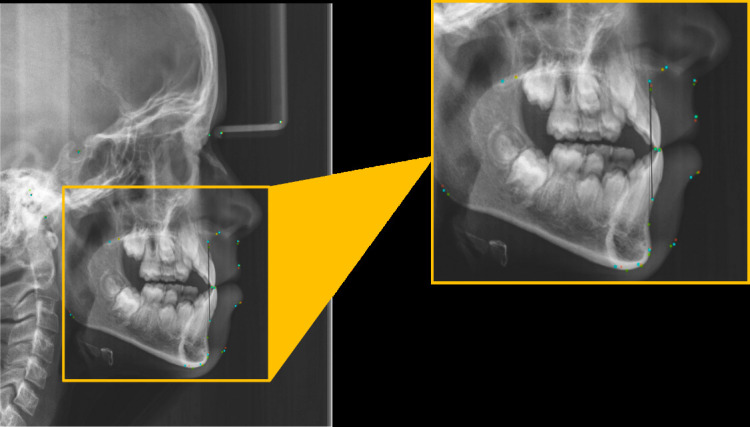
Descriptive statistics parameters such as mean, SD, standard error of the mean (SEM), minimum (min) and maximum (max) of EDs between the corresponding landmarks of both software programs were determined (Table 5). The literature states that 2–4 mm is acceptable ^4,24 ; however, a surprisingly large discrepancy was noted. This was concerning as visually the landmarks’ locations between the two systems were in close approximation (Figure 5). The greatest ED was observed for L18 (anterior nasal spine) (92.43 mm). The next largest ED was observed for L16 (soft tissue pognion) (87.63) followed by L2 (nasion) (52.36). The smallest ED was observed for L15 (subnasale). The minimum and maximum range was 2.34 mm and 76.01 mm, respectively.

Table 5.

Mean value of the Euclidean distances

Landmark	Mean	±SD	±SEM	Min	Max
L1	6.19	2.02	0.0998	1,99	17,9
L2	8.75	3.76	0.1859	0,58	52,36
L3	9.64	3.16	0.1562	1,46	21,39
L4	8.98	3.41	0.1686	0,57	23,37
L5	10.57	3.75	0.1854	1,92	24,24
L6	10.84	4.15	0.2052	1,11	29,92
L7	10.43	4.09	0.2022	2,07	29,23
L8	11.29	4.38	0.2165	1,05	29,08
L9	11.28	4.25	0.2101	1,96	28,87
L10	10.43	5.81	0.2872	0,42	31,22
L11	10.2	3.93	0.1943	1,76	24,93
L12	10.59	4.08	0.2017	1,14	26,92
L13	9.65	4.1	0.2027	1,61	27,28
L14	11.09	4.69	0.2319	0,81	42,3
L15	9.6	4.62	0.2284	0,22	54,47
L16	10.66	5.4	0.2670	2,56	87,63
L17	7.66	3.71	0.1834	0,50	50,06
L18	8.88	5.55	0.2744	1,09	92,43
L19	7.10	2.65	0.1310	0,54	16,42

Max, maximum; Min, minimum; SD, standard deviation; SEM, standard error of the mean.

Figure 5.

Superimposed image comparing the landmarks detected by Software B (green) and human examination using Software A (red).

The SD represents the difference ± value from the mean Euclidean value of each landmark of the 409 cephalograms. The SEM values from the ED are represented in Table 6. The SEM represents the precision of how close the value is to the whole sample size of 409 cephalograms for each landmark. The small values of the SEM illustrated that the SEM is closely related with a narrow distribution to the SD. A small value of mean error represented acceptable landmark detection results in the case of cephalometric analysis.

Table 6.

SD and SEM

Landmark	Software B x		Software A x		Software B y		Software A y
	SD	SEM	SD	SEM	SD	SEM	SD	SEM
L1	5.6	0.2769	5.5	0.2720	6.11	0.3021	5.72	0.2828
L2	7.86	0.3887	7.35	0.3634	9.67	0.4782	9.2	0.4549
L3	5.97	0.2952	6.19	0.3061	8.17	0.4040	7.93	0.3921
L4	5.66	0.2799	3.77	0.1864	6.63	0.3278	5.22	0.2581
L5	6.77	0.3348	7.16	0.3540	9.08	0.4490	8.9	0.4401
L6	9.12	0.4510	8.91	0.4406	9.88	0.4885	10.22	0.5053
L7	10.4	0.5142	10.04	0.4964	10.49	0.5187	10.53	0.5207
L8	10.83	0.5355	10.17	0.5029	10.29	0.5088	10.37	0.5128
L9	10.69	0.5286	10.22	0.5053	10.48	0.5182	10.54	0.5212
L10	8.72	0.4312	6.52	0.3224	9.09	0.4495	6.9	0.3412
L11	8.25	0.4079	8.45	0.4178	9.54	0.4717	9.68	0.4786
L12	8.48	0.4193	8.63	0.4267	9.71	0.4801	9.88	0.4885
L13	7.81	0.3862	8.13	0.4020	10.5	0.5192	10.57	0.5227
L14	8.78	0.4341	8.9	0.4401	10.46	0.5172	10.53	0.5207
L15	7.36	0.3639	7.96	0.3936	9.96	0.4925	10.52	0.5202
L16	9.98	0.4935	10.49	0.5187	10.97	0.5424	10.95	0.5414
L17	5.68	0.2809	6.12	0.3026	6.31	0.3120	6.2	0.3066
L18	6.62	0.3273	8.34	0.4124	9.27	0.4584	9.25	0.4574
L19	5.99	0.2962	4.74	0.2344	6.32	0.3125	5.23	0.2586

SD, standard deviation; SEM, standard error of the mean.

Wilcoxon rank test and Bland–Altman plots

Indicating the truth of the null hypothesis, there was no significant difference between x- nor y-values of both software programs (Table 7) (p > 0.05). The y coordinate of L2 (Nasion) in software B was presented with a significant difference (p = 0.000031) concerning the y-values obtained in software A.

Table 7.

Comparison of p values between vertical and horizontal planes

Landmark	X value for Software A vs B	Y value for Software A vs B
L1	4.64	7.21
L2	1.11	0.000031
L3	1.03	8.51
L4	1.04	3.50
L5	8.08	7.28
L6	4.73	1.92
L7	4.00	2.66
L8	9.19	6.46
L9	4.46	8.66
L10	2.11	5.71
L11	5.72	3.73
L12	4.24	2.97
L13	4.39	1.49
L14	7.07	2.56
L15	1.65	2.61
L16	1.18	2.86
L17	8.47	4.18
L18	1.21	3.42
L19	1.07	5.73

Large variations of the x- and y-coordinates occurred. L8 (Menton) and L5 (Point A) were the most reliable landmarks in the horizontal plane (p = 9.19 and 8.08, respectively). L9 (Orbitale) was the most reliable in the vertical plane (p-value of 8.66). L2 in the vertical dimension (y-value) presented with a significant difference (p = 0.000031).

Orbitale was more inaccurate in the horizontal plane, most likely the result of the left and right images of the orbits being more closely aligned vertically than anteroposteriorly (p for x-axis = 1.03, p for y-axis = 8.51). Alternatively, articulare was more imprecise vertically (p for x-axis = 1.07, p for y-axis = 5.73) since this landmark is defined as the most posterior point on the neck of the vertically oriented condyle. The convoluted route of the ear canals creates multiple vertically overlapping radiolucent structures, which was likely a contributory factor in the imprecision of identification of Porion in the vertical direction (p-value for x-axis = 1.04, p-value for y-axis = 3.50). Uncertainty in the detection of Gonion may result from the difficulty of establishing this landmark’s position along a curved anatomical structure (SD = 5.81).

Bland–Altman

Bland–Altman analysis was carried out on L2 (Nasion) due to the y-value statistical analysis with the Wilcoxon showing a significant difference between the two programs. L16 (Soft tissue pogonion) was also analyzed for comparison. The interpretation of the Bland–Altman was limited to L1 (Sella), L2 (Nasion) and L16 (Soft tissue pogonion) (Figures 6–11). These landmarks were identified based on the smallest ED of L1 which was the smallest (6.19), and L16 a soft tissue landmark (10.66), where the Wilcoxon statistical significance for the y-coordinates of L2 was determined to be p = 0.000031.

Figure 6.

Bland–Altman graph for Landmark 1, x value.

Figure 7.

Bland–Altman graph for Landmark 1, y value.

Figure 8.

Bland–Altman graph for Landmark x value.

Figure 9.

Bland–Altman graph for Landmark 2, y value.

Figure 10.

Bland–Altman graph for Landmark 1, x value.

Figure 11.

Bland–Altman graph for Landmark 1, y value.

The comparison and interpretation of the Bland–Altman graphs provided insight to why L2; y-values presented with a significant difference. As per Table 8, the number of y-coordinates above the upper limit of agreement (ULOA) is 99. This large number of coordinates resulted in the statistical significance noted for the y-coordinate for L2. The ULOA was 6.402 and the difference in the coordinates between both programs was up to 28.98. Software B had much larger y-coordinates for L2, resulting in the result that there is a significant difference with the Wilcoxon test for the BoneFinder^® coordinates in relation to Software A.

Table 8.

The distribution of the difference values for the various landmarks, based on the (x,y) coordinates

Landmark and coordinate	Below LLOA	Between LLOA and ULOA	Above ULOA	Around the bias line not crossing any limits—above bias line	Around the bias line not crossing any limits—below bias line
L1 X-Value	409	4	0	188	218
L2 X-Value	376	29	4	119	257
L16 X-Value	409	0	0	185	224
L1 Y-Value	135	273	1	193	80
L2 Y-Value	128	182	99	116	66
L16 Y-Value	392	17	0	178	214

LLOA, lower limit of agreement; ULOA, upper limit of agreement.

When looking at the race of a sample of 10 cephalograms that were around the bias, and the large values above the ULOA respectively; the majority was of mixed ethnicity. L2 is usually a reliable landmark as it is situated at a well-defined anatomic point at the intersection of frontal and nasal bones. This region was dark and on our sample of radiographs. Patient tilting also resulted in the landmark requiring interpretation.

Incidental findings

Incidental findings are becoming directly proportional to the advancement of medical technologies used in treatment and research. ²⁵ Attempts to explain the large discrepancy in the EDs were actively pursued but were not the primary reason for the study. These attempts included:

1. Different file inputs

Software B provided coordinates in millimeters if the file input was in DICOM format, whereas JPEG files produced coordinates in pixels. In view of this, and the consensus that DICOM files have the highest image quality, ^26–29 DICOM files were used in both methods. However, it resulted in large discrepancies in the ED. An incidental finding revealed that if one compared the same cephalogram using Software B coordinates (using a DICOM file) with the Software A coordinates (JPEG file), the results were more comparable to those in the literature, i.e. within the accepted 2 mm range. ^17,22 The mean ED of Software A JPEG and Software B DICOM was within the accepted range of 2.15 mm, whereas the mean ED of Software B DICOM and Software A DICOM was 8.49 mm.

Table 9 shows that Software B provides deterministic results, i.e. the coordinates output would be the same, no matter how many times the same image is imported into the software. Interestingly, when a JPEG image was imported into Software A, it yielded different coordinates from those of the DICOM file. This was contradictory to the results of Saez et al ³⁰ and Saghaie and Ghaffari ³¹ who evaluated the influence of DICOM and JPEG formats on cephalometric landmarks detection and found JPEG file formats to be reliable.

Table 9.

A comparison of file inputs and their respective Euclidean distances

Software B DICOM		Software A JPEG		Software B DICOM		Software A DICOM		ED1	ED2
X	Y	X	Y	X	Y	X	Y
56.0692	84.7893	53.8	−86.0	56.0692	84.7893	51.4	−83.1	2,57	2,57
124.513	57.8378	124.0	−58.7	124.513	57.8378	116.8	−57.1	1	7,75
116.972	92.6589	114.4	−92.7	116.972	92.6589	103.9	−92.4	2,57	13,07
39.4534	107.933	32.8	−102.5	39.4534	107.933	33.2	−103.4	8,59	7,72
138.273	121.236	137.1	−120.5	138.273	121.236	130.9	−117.5	1,38	8,27
141.43	159.992	139.8	−159.7	141.43	159.992	134.0	−153.5	1,66	9,87
147.175	176.163	145.7	−175.5	147.175	176.163	139.5	−169.3	1,62	10,3
142.089	183.857	141.3	−183.1	142.089	183.857	135.2	−177.2	1,09	9,58
146.032	180.966	145.0	−180.2	146.032	180.966	138.8	−173.8	1,29	10,18
67.9345	169.588	65.8	−171.6	67.9345	169.588	60.9	−165.0	2,93	8,4
143.968	143.858	142.8	−144.7	143.968	143.858	136.4	−139.7	1,44	8,64
146.584	144.692	145.0	−144.4	146.584	144.692	139.2	−139.2	1,61	9,2
160.239	128.198	160.8	−130.6	160.239	128.198	154.1	−127.5	2,47	6,18
158.483	148.165	157.1	−147.9	158.483	148.165	151.7	−140.9	1,41	9,94
155.459	116.939	155.1	−116.1	155.459	116.939	148.1	−112.7	0,91	8,49
162.005	172.31	160.3	−175.5	162.005	172.31	153.8	−172.6	3,62	8,21
84.5971	126.213	86.6	−126.9	84.5971	126.213	79.5	−122.0	2,12	6,61
142.189	114.68	140.8	−114.1	142.189	114.68	134.7	−110.8	1,51	8,43
48.8331	123.398	47.8	−123.7	48.8331	123.398	43.0	−118.0	1,08	7,95

ED1, Euclidean Distance (Software B DICOM and Software A JPEG); ED2, Euclidean Distance (Software B DICOM and Software A DICOM).

2. Adjusting the ruler calibration in Software A

As described in the methodology, a ruler length of 30 mm was used. This is in accordance with the real length of the corner points of the nasion-positioning rod. This was needed for image calibration since no calibration ruler was included during the acquisition of the image. When re-evaluating Software A’s parameters, it was apparent that changes to the calibration ruler significantly changed the results. The possibility of inaccurate measurement of the nasion-positioning rod was explored. Table 10 shows that when this distance was changed to 31 mm, it considerably altered the output. In this study, the lack of a ruler during the acquisition stage meant that calibration needed to be performed using two fixed points. This measurement of a known distance (30 mm) between the two fixed corner points of the nasion-guiding rod on the screen was chosen. However, this also could have introduced random error as the placement of the mouse-driven cursor was highly sensitive. The actual process of the calibration was not perfectly repeatable; therefore, uncertainty may have been introduced.

Table 10.

Changes of ruler calibration

Landmarks	Software A				Software B		E1	E2
	30 mm		31 mm
	X	Y	X	Y	X	Y
L1	57.8	75.4	58,5	75,8	59.3796	79.0643	3,99	3,38
L2	131.9	70.5	133,5	71,2	132.361	70.1415	0,58	1,55
L3	112.8	99.3	115,4	100,5	120.138	100.923	7,52	4,76
L4	28.0	93.5	27,1	92,4	33.0467	99.824	8,09	9,51
L5	129.3	132.1	131,3	133,5	131.298	137.655	5,9	4,16
L6	117.9	174.7	119,8	176,5	126.251	182.461	11,4	8,78
L7	118.4	192.3	120,1	195,4	125.675	198.117	9,31	6,2
L8	110.7	198.8	112,3	201,7	117.724	204.58	9,1	6,14
L9	116.0	197.6	116,4	200,7	123.112	202.761	8,79	7,02
L10	39.4	161.9	42,3	166	48.1837	165.141	9,36	5,95
L11	123.7	157.0	126	159,7	135.644	160.908	12,57	9,72
L12	129.3	159.9	130,8	161,9	138.028	162.627	9,14	7,26
L13	146.9	145.9	147,7	146,5	151.633	148.325	5,32	4,34
L14	138.0	168.1	138,7	169,9	147.621	177.573	13,5	11,77
L15	150.3	131.2	154,6	131,1	145.338	135.312	6,44	10,17
L16	131.9	191.8	133,8	191,9	139.775	196.754	9,3	7,7
L17	74.4	125.4	77	125,9	81.2463	128.275	7,43	4,87
L18	136.8	128.5	138,7	130,1	134.155	130.224	3,16	4,55
L19	35.8	113.3	36,2	116,1	42.5032	115.531	7,06	6,33

E1, Euclidean Distance (Software A Original calibration of 30 mm and Software B ; E2, Euclidean Distance (Software A New calibration of 31 mm and Software B).

Record number 10 was used.

3. Image alignment

When the cephalogram was dragged into the image box in Software A, the automatic alignment of the image was used (Figure 12) (Scenario A). To assess whether the alignment changed the coordinate outputs, the image was then re-aligned so that the cephalogram image border and the boundary box corresponded (Figure 12) (Scenario B). The coordinates from these scenarios were exported and as anticipated the coordinates did indeed differ. Furthermore, the ED discrepancy still existed (Table 11).

Figure 12.

Scenario a: The automatic alignment places the cephalogram image border outside the black boundary (dotted border lies outside the black solid line). Scenario b: The image was aligned so that the cephalogram image border and the boundary box corresponded (dotted line).

Table 11.

Comparison of the Euclidean distance with changes of alignment

Landmarks	Software A Autoaligned		Software A Manually aligned		Software B		E1	E2
	X	Y	X	Y	X	Y
L1	57.8	−75.4	57.8	−73.2	59.3796	79.0643	3.99	6.07
L2	131.9	−70.5	129.3	−68.0	132.361	70.1415	0.58	3.74
L3	112.8	−99.3	112.0	−96.6	120.138	100.923	7.52	9.21
L4	28.0	−93.5	28.3	−86.0	33.0467	99.824	8.09	14.62
L5	129.3	−132.1	128.4	−127.4	131.298	137.655	5.9	10.66
L6	117.9	−174.7	116.7	−169.1	126.251	182.461	11.4	16.42
L7	118.4	−192.3	116.9	−186.4	125.675	198.117	9.31	14.64
L8	110.7	−198.8	109.9	−193.4	117.724	204.58	9.1	13.65
L9	116.0	−197.6	114.6	−191.5	123.112	202.761	8.79	14.12
L10	39.4	−161.9	40.7	−156.9	48.1837	165.141	9.36	11.13
L11	123.7	−157.0	122.1	−152.9	135.644	160.908	12.57	15.73
L12	129.3	−159.9	127.5	−155.7	138.028	162.627	9.14	12.6
L13	146.9	−145.9	143.8	−139.8	151.633	148.325	5.32	11.58
L14	138.0	−168.1	134.7	−163.7	147.621	177.573	13.5	18.96
L15	150.3	−131.2	150.9	−124.9	145.338	135.312	6.44	11.8
L16	131.9	−191.8	130.5	−184.3	139.775	196.754	9.3	15.53
L17	74.4	−125.4	75.3	−120.4	81.2463	128.275	7.43	9.87
L18	136.8	−128.5	135.0	−124.4	134.155	130.224	3.16	5.88
L19	35.8	−113.3	36.3	−111.3	42.5032	115.531	7.06	7.51

E1, Euclidean Distance (Software A Original calibration of 30mm and Software B); E2, Euclidean Distance (Software A New calibration of 31mm and Software B).

Record 10 was used.

Discussion

Demographics

A large component of this study sample consisted of colored/mixed race individuals (59.66%) and blacks (9.78%). As was prevalent in 1995 ³² and now, black and colored patients are presenting in increasing numbers for orthodontic treatment. It is important to note that patients of mixed ancestry can present with different skeletal patterns contributing to different landmark norms. Each continent or country will have differences in cephalometric values among various ethnic groups. A study in 1983 determined clinical cephalometric values applicable to the Cape Colored community and is the only comparative study performed to date. ²³ No comparative cephalometric studies have been performed on the South African Cape Colored community. An evaluation of the mean cephalometric values for black South African adults in the Western Cape region of South Africa was last conducted in 1997. ³³ In South Africa, particularly, years of integration of ethnic groups have taken place leading to difficulties in characterizing those groups based on the norms. ³³ Literature on South African population groups is outdated. The findings of this current study motivate the development of cephalometric norms to provide a closer approximation of the profiles of the South African population.

Errors

Inconsistency in landmark identification is the most central source of random errors in cephalometry. ³⁴ Factors inducing random errors include image quality, landmark definition, reproducibility of landmark location, operator experience, and recording procedure. ^35,36 Efforts to minimize random error were made by ensuring there was minimal subjectivity, therefore only one examiner performed the landmark detections. ¹² Examiner 1 had 3 years of experience in maxillofacial radiology. Other factors possibly affecting intraexaminer agreement included orthodontic experience and time constraints. Some landmarks also show a wider variation in localization. Landmarks such as Gonion, Porion, Orbitale, and the lower incisor apex may be difficult to identify due to their superimposition between bilateral anatomical structures. ³⁷ Gonion, porion and orbitale also showed variation in this study’s interexaminer tests.

Errors can also be induced by anatomical variations. This can be explained by using interval 2, L17 (PNS) y-coordinate (ICC = 0.56) as an example (Figure 13). Due to the maxillary third molars that are commonly unerupted, they can obscure the detection of PNS. Consequently, the location of this landmark moves from “identifiable” to requiring interpretation—subjectivity and experience play a big role here. This shows that variations can still exist within a single examiner and between different examiners. This substantiates the need for an objective AI solution.

Figure 13.

Comparison of PNS landmark detection. The unerupted third molar superimposed on the landmark region renders the PNS indifferentiable. All examiners detected PNS at varying points—primary researcher (red); chief radiographer (green) and orthodontist (blue) using Software A.

Software A

It is important to note that Software A is used more often than other digital cephalometric software programs. ¹² The most surprising aspect to emerge from the data was the large ED, where it was consistently greater than 4 mm. This was concerning as visually the landmarks’ locations between the two systems were in close approximation. Unfortunately, changing the measuring technique (i.e. the software parameters) was not possible. Therefore, it is difficult to know the type of systematic error that could be present. A suggested contributing factor could be the reference frame used in Software A. A reference frame refers to the coordinate system used whereby the origin, orientation and scale are defined by a set of reference points. ⁵ Very little was found in the literature on the question of reference frames concerning cephalometric studies. Condylion was not identified at its true anatomical position but was selected arbitrarily to be used as the center of origin to determine the (x,y) coordinates of the other landmarks. This also may have introduced a calibration error.

Software B

Software B is based on a machine learning approach; however, the training data set was limited to 400 digital cephalograms. ⁵ AI is only as smart as the size of the data set it was trained on. ^1,19 It was approximated that at least 2300 learning data sets would be required to develop accurate and clinically applicable AI in orthodontics. ¹⁹ Furthermore, Software B may have also inherited some of the inaccuracies from the manual training data. (5) AI aims to be objective, but to identify landmarks, training needs to be annotated by humans. ¹ This in turn can be subjective, depending on the level of experience and knowledge of the examiners.

Landmarks and case examples

In this data set, there were two kinds of landmarks: (a) anatomic or identifiable landmarks and (b) interpreted landmarks (Figure 14a–h). The former landmarks refer to anatomic structures that were clearly recognized and the latter are derived from neighboring anatomic structures and require interpretation which may be subjective. ^38,39 Automated methods also suffered from inaccurate localization. The difficulty in the localization of L10 (Gonion) has been reported. ^5,40 This is usually caused by the asymmetry of the mandible. ³⁹ In this study, Gonion also showed the greatest SD (5.81).

Figure 14.

Right—landmark detection with Software A; Middle—landmark detection with Software B; Left—Superimposed images. (a) Effect of improper lip tension; improper lip tension shifts landmark soft tissue pogonion to a position midway (green) between the human detected pogonion (red) and the lower lip. (b) Effect of crowded anterior teeth; Software B did not select the most inferior aspect of the incisal tip of the most labially places maxillary incisor. (c) Differences of the automatically detected ANS and A point. (d) Gonion landmark; a discrepancy was noted between the human-detected landmark and the automatically detected landmark. (e) Bilateral rule for detecting gonion; Gonion is detected on the most inferior and posterior border (white dashed line) of the mandible. (f) Detection of Orbitale; discrepancy noted in detecting orbitale. (g) Detection of nasion; frontonasal suture is not easily detectable in this case. Discrepancy of human-detected landmark for nasion, and automatically detected landmark. (h) Detection of articulare; interpretation required to determine location of articulare. Software B did not utilize the bilateral rule.

Some landmarks had a higher ED (Na, ANS, soft-tissue pogonion). Possible reasons for this include: (1) inadequate image quality, (2) anatomical variations and (3) local feature alterations. ⁴¹ Image quality varies regionally in cephalograms, and as a result, some image regions facilitate accurate localization, whereas others do not. Therefore, including only those images with perfect overall quality in which most of the landmarks are clearly identifiable was unfeasible. Local features can also be altered by the nasion positioning rod. The anterior nasal spine tends to be overexposed due to its delicate structure. Figure 14h shows that the frontonasal suture is not easily detected. This can be due to the superimposition of the upper eyelid nasion point is usually superimposed by the upper eyelid. The detection of some landmarks, such as nasion, ANS and orbitales, located at the superimposed structures sometimes cannot be improved even by applying filters.

Errors can also be induced by anatomical variations. In Figure 14a, the discrepancy between the soft tissue pogonion determined by the researcher and the automatically detected pogonion locations is displayed. The disparity is produced by abnormal lip tension in individuals with forcefully corrected lip incompetence, which distorts the chin profile causing soft tissue pogonion to deviate. ^41,42

Some landmarks suffer from a combination of poor definition due to superimposition and uncertain interpretation. For example, articulare (Figure 14h) is composed of three independent bones: the inferior surface of the cranial base, and the posterior outlines of the mandibular rami and condyles. As per the bilateral rule, the average part of bilateral structures was “traced” before locating the landmark at the midpoint of the tracing line.

Limitations

The sample size was relatively small due to the lack of records complying with the inclusion and exclusion criteria. Other factors contributing to the identification error are examiner experience, landmark definition, image resolution, operator fatigue and subjectivity.

A common occurrence in academic institutions is when students utilize the equipment and regularly misplace the metal rulers. Regular replacement of equipment in a public health center is usually requested by clinical academic staff but can only be approved by hospital management. The ruler was missing for an extended period during the time of the study, and we were unable to order a new ruler during the Covid-19 pandemic. The re-exposure of patients for the sole purpose of obtaining data for a study would be unethical, as a result, the cephalograms lacking the ruler were utilized and efforts to calibrate the image were made. Whilst the calibration process was subject to sensitivity, the Orthodontic and Radiology Department, was in the interim, following the protocol of using the two corner points of the fixed plastic nasion rod.

However, this also could have introduced random error as the placement of the mouse-driven cursor was highly sensitive. A metal ruler would have projected a sharper image than the image of the plastic nasion rod, which led to softer edges. The actual process of the calibration was also not perfectly repeatable; therefore, uncertainty was introduced through the calibration process. The results and limitations of this study was used to expedite the request for a ruler. Taken together, this study emphasizes the need for a metal ruler in cephalometric calibration.

Software B’s training set consisted of patient cephalograms between the ages of 7–76. If a European or Asian data set was utilized, it may have influenced the training data set. As noted earlier, craniofacial patterns differ in patients of mixed ethnicities. ³⁵ This was the first time Software B was used on a South African population, and this may have also been attributed to the discrepancies observed.

Recommendations

This study intended to provide a means for precise detection of cephalometric landmarks within a South African context. This was to substantiate the benefit of implementing fully automated cephalometric landmark detection programmes in orthodontic practices that will ultimately assist with workflow and improve treatment planning with increased precision. The results of this study were very sensitive to several variables. Therefore, several questions remain unanswered at present. However, there is abundant room for further progress in determining whether AI can replace computer-assisted landmark detection approaches and contribute to the growth of AI in Africa. A number of possible future studies using the same experimental setup are apparent: (1) a study similar to this one should be carried out with correctly calibrated cephalometric images to explore Software B’s reliability within a South African context, (2) the data set used by Lindner et al ⁵ in their development of Software A could be used to compare the precision to Software A. The investigation of association of reference frames can also be investigated.

With the change in Euclidean distances that occurred with various file inputs, it is likely that connections exist between the type of file input and their respective image data. This finding, while preliminary, advocates for more research on this topic to be undertaken before the association between file inputs and coordinate outputs is more clearly understood.

There is also a lack of robustness in available training data sets, and this is influenced by the inaccessibility of standard and calibrated data sets. It would be beneficial to create an open standard South African data set with the ground truth marked and validated by experienced clinicians for future research into automated landmark detection. Due to the significant variation in anatomical features among different ethnic groups, the data sets would also need to be representative of each ethnic group. Data sets are usually trained according to inclusion and exclusion criteria, however, distortion to the skull caused by diseases etc need to also be included. This will enable an AI system to detect landmarks on anomalous skulls. Before AI can be fully adopted in a clinical setting in South Africa, further studies determining South African cephalometric norms should be carried out. A better understanding of this would also contribute to a South African data set of cephalograms.

Conclusion

It was difficult to draw a robust comparison, as several parameters led to fluctuating results. These results provide important insights as well as raises more questions about AI and computer-assisted approaches. In conclusion, there was no significant difference between the two software programs regarding the precision of landmark detection. This study also emphasized the need for a metal ruler in cephalometric calibration. Taken together, these findings suggest a promising role for the future of AI in cephalometry research that can be translated to the clinical arena.

REFERENCES

- 1. Silva TP, Hughes MM, Menezes L dos S, de Melo M de FB, Freitas PHL de, Takeshita WM. Artificial intelligence-based Cephalometric landmark Annotation and measurements according to Arnett’s analysis: can we trust a Bot to do that Dentomaxillofacial Radiology 2022; 51(. doi: 10.1259/dmfr.20200548 [DOI] [PMC free article] [PubMed] [Google Scholar]
- 2. Ongkosuwito EM, Katsaros C, van ’t Hof MA, Bodegom JC, Kuijpers-Jagtman AM. The reproducibility of Cephalometric measurements: a comparison of analogue and Digital methods. Eur J Orthod 2002; 24: 655–65. doi: 10.1093/ejo/24.6.655 [DOI] [PubMed] [Google Scholar]
- 3. Shahidi S, Bahrampour E, Soltanimehr E, Zamani A, Oshagh M, Moattari M, et al. The accuracy of a designed software for automated localization of Craniofacial landmarks on CBCT images. BMC Med Imaging 2014; 14: 1–8: 32. doi: 10.1186/1471-2342-14-32 [DOI] [PMC free article] [PubMed] [Google Scholar]
- 4. Durão APR, Morosolli A, Pittayapat P, Bolstad N, Ferreira AP, Jacobs R. Cephalometric landmark variability among orthodontists and Dentomaxillofacial Radiologists: A comparative study. Imaging Sci Dent 2015; 45: 213–20. doi: 10.5624/isd.2015.45.4.213 [DOI] [PMC free article] [PubMed] [Google Scholar]
- 5. Lindner C, Wang CW, Huang CT, Li CH, Chang SW, Cootes TF. Fully automatic system for accurate Localisation and analysis of Cephalometric landmarks in lateral Cephalograms. Sci Rep 2016; 6: 1–10. doi: 10.1038/srep33581 [DOI] [PMC free article] [PubMed] [Google Scholar]
- 6. Deshmukh S. Artificial intelligence in dentistry. J Int Clin Dent Res Organ 2018; 10: 47. doi: 10.4103/jicdro.jicdro_17_18 [DOI] [Google Scholar]
- 7. Tang A, Tam R, Cadrin-Chênevert A, Guest W, Chong J, Barfett J, et al. Canadian Association of Radiologists white paper on artificial intelligence in Radiology. Can Assoc Radiol J 2018; 69: 120–35. doi: 10.1016/j.carj.2018.02.002 [DOI] [PubMed] [Google Scholar]
- 8. Yaji A, Prasad S, Pai A. Artificial intelligence in Dento-Maxillofacial Radiology. Acta Sci Dent Sci 2019; 3: 2581–4893. [Google Scholar]
- 9. Miloro M, Borba AM, Ribeiro-Junior O, Naclério-Homem MG, Jungner M. Is there consistency in Cephalometric landmark identification amongst oral and Maxillofacial Surgeons International Journal of Oral and Maxillofacial Surgery 2014; 43: 445–53. doi: 10.1016/j.ijom.2013.08.007 [DOI] [PubMed] [Google Scholar]
- 10. Hwang H-W, Park J-H, Moon J-H, Yu Y, Kim H, Her S-B, et al. Automated identification of Cephalometric landmarks: part 2-might it be better than human. Angle Orthod 2019; 00: 1–8. doi: 10.2319/022019-129.1 [DOI] [PMC free article] [PubMed] [Google Scholar]
- 11. Department of Orthodontics, Faculty of Dentistry, Trakya University, Edirne, Turkey, Meric P, Naoumova J, Specialist Clinic of Orthodontics, University Clinics of Odontology, Public Dental Service, Västra Götaland Region, Gothenburg, Sweden . Web-based fully automated Cephalometric analysis: comparisons between App-aided, computerized, and manual tracings. Turk J Orthod 2020; 33: 142–49. doi: 10.5152/TurkJOrthod.2020.20062 [DOI] [PMC free article] [PubMed] [Google Scholar]
- 12. Anuwongnukroh N, Dechkunakorn S, Damrongsri S, Nilwarat C, Pudpong N, Radomsutthisarn W, et al. Assessment of the reliability of automatic Cephalometric analysis software. IJMERR 2017; 6: 61–65. doi: 10.18178/ijmerr.7.1.61-65 [DOI] [Google Scholar]
- 13. Lindner C, Wang CW, Huang CT, Li CH, Chang SW, Cootes TF. Fully automatic system for accurate Localisation and analysis of Cephalometric landmarks in lateral Cephalograms. Sci Rep 2016; 6: 33581. doi: 10.1038/srep33581 [DOI] [PMC free article] [PubMed] [Google Scholar]
- 14. INTERACT (Lab Suite Version 2015, v 1.5) Mangold International Germany. Available from: www.mangold-international.com (accessed 11 Feb 2021)
- 15. Aksakalli S, Yilanci H, Gorukmez E, Ramoglu SI. Reliability assessment of orthodontic Apps for Cephalometrics. Turk J Orthod 2017; 29: 98–102. doi: 10.5152/TurkJOrthod.2016.1618 [DOI] [PMC free article] [PubMed] [Google Scholar]
- 16. [R Core Team]. R: A Language and Environment for Statistical Computing. Vienna, Austria: R Foundation for Statistical Computing, Available from: https://www.R-project.org [Google Scholar]
- 17. Koo TK, Li MY. A guideline of selecting and reporting Intraclass correlation coefficients for reliability research. Journal of Chiropractic Medicine 2016; 15: 155–63. doi: 10.1016/j.jcm.2016.02.012 [DOI] [PMC free article] [PubMed] [Google Scholar]
- 18. Katkar RA, Kummet C, Dawson D, Moreno Uribe L, Allareddy V, Finkelstein M, et al. Comparison of observer reliability of three-dimensional Cephalometric landmark identification on subject images from Galileos and I-CAT cone beam CT. Dentomaxillofac Radiol 2013; 42: 20130059. doi: 10.1259/dmfr.20130059 [DOI] [PMC free article] [PubMed] [Google Scholar]
- 19. Wang C-W, Huang C-T, Lee J-H, Li C-H, Chang S-W, Siao M-J, et al. A benchmark for comparison of dental radiography analysis Algorithms. Med Image Anal 2016; 31: 63–76. doi: 10.1016/j.media.2016.02.004 [DOI] [PubMed] [Google Scholar]
- 20. Park J-H, Hwang H-W, Moon J-H, Yu Y, Kim H, Her S-B, et al. Automated identification of Cephalometric landmarks: part 1—comparisons between the latest deep-learning methods Yolov3 and SSD Angle Orthod 2019; 89: 903–9. doi: 10.2319/022019-127.1 [DOI] [PMC free article] [PubMed] [Google Scholar]
- 21. Moon JH, Hwang HW, Yu Y, Kim MG, Donatelli RE, Lee SJ. How much deep learning is enough for automatic identification to be reliable? A Cephalometric example Angle Orthod 2020; 90: 823–30. doi: 10.2319/021920-116.1 [DOI] [PMC free article] [PubMed] [Google Scholar]
- 22. ISO. ISO 5725-1 . Accuracy (trueness and precision) of measurement methods andresults–Part 1: General principles and definitions. . Geneva: 1998. Available from: https://www.iso.org/obp/ui/#iso:std:iso:5725:-1:ed-1:v1:en [Google Scholar]
- 23. Menditto A, Patriarca M, Magnusson B. Understanding the meaning of accuracy, Trueness and precision. Accred Qual Assur 2007; 12: 45–47. doi: 10.1007/s00769-006-0191-z [DOI] [Google Scholar]
- 24. Juneja M, Garg P, Kaur R, Manocha P, Prateek S, et al. A review on Cephalometric landmark detection techniques. Biomedical Signal Processing and Control 2021; 66: 102486. doi: 10.1016/j.bspc.2021.102486 [DOI] [Google Scholar]
- 25. Seedat AK. Cephalometric analysis of a group of Cape Coloureds. J Dent Assocaition South Africa 1983; 38: 673–75. [PubMed] [Google Scholar]
- 26. Miloro M, Borba AM, Ribeiro-Junior O, Naclério-Homem MG, Jungner M. Is there consistency in Cephalometric landmark identification amongst oral and Maxillofacial Surgeons? Int J Oral Maxillofac Surg 2014; 43: 445–53. doi: 10.1016/j.ijom.2013.08.007 [DOI] [PubMed] [Google Scholar]
- 27. Ells C, Thombs BD. The ethics of how to manage incidental findings. CMAJ 2014; 186: 655–56. doi: 10.1503/cmaj.140136 [DOI] [PMC free article] [PubMed] [Google Scholar]
- 28. Graham RNJ, Perriss RW, Scarsbrook AF. DICOM Demystified: A review of Digital file formats and their use in radiological practice. Clin Radiol 2005; 60: 1133–40. doi: 10.1016/j.crad.2005.07.003 [DOI] [PubMed] [Google Scholar]
- 29. Faccioli N, Perandini S, Comai A, D’Onofrio M, Pozzi Mucelli R. Proper use of common image file formats in handling radiological images. Radiol Med 2009; 114: 484–95. doi: 10.1007/s11547-009-0378-6 [DOI] [PubMed] [Google Scholar]
- 30. Varma DR. Managing DICOM images: tips and tricks for the Radiologist. Indian J Radiol Imaging 2012; 22: 4–13. doi: 10.4103/0971-3026.95396 [DOI] [PMC free article] [PubMed] [Google Scholar]
- 31. Burgess J. Digital DICOM in dentistry. Open Dent J 2015; 9: 330–36. doi: 10.2174/1874210601509010330 [DOI] [PMC free article] [PubMed] [Google Scholar]
- 32. Saez DM, Bommarito S, Sannomiya EK. Reproducibility of Cephalometric landmarks on Posteroanterior Digital Radiographs using DICOM and JPEG formats. Oral Radiol 2016; 32: 79–86. doi: 10.1007/s11282-015-0217-5 [DOI] [Google Scholar]
- 33. Saghaie S, Ghaffari R. Effect of image compression of Digital lateral Cephalograms on the reproducibility of Cephalometric points. Dent Res J (Isfahan) 2014; 11: 27–31. [PMC free article] [PubMed] [Google Scholar]
- 34. Naidoo LCD, Miles LP. An evaluation of the mean Cephalometric values for Orthognathic surgery for black South African adults. Part I: Hard Tissue J Dent Assoc South Africa 1997; 52: 495–502. [PubMed] [Google Scholar]
- 35. Barter MA, Evans WG, Smit GL, Becker PJ. Cephalometric analysis of a Sotho-Tswana group. J Dent Assoc South Africa 1995; 50: 539–44. [PubMed] [Google Scholar]
- 36. Kula K, Ghoneima A.. A Perspective on Norms and Standards. In: Kula K, Ghoneima A. Cephalometry in orthodontics: 2D and 3D 1st ed. Quintessence Publishing Co, Inc; 2018. p. 83–6. [Google Scholar]
- 37. Leonardi R, Giordano D, Maiorana F, Spampinato C. Automatic Cephalometric analysis: A systematic review. Angle Orthod 2008; 78: 145–51. doi: 10.2319/120506-491.1 [DOI] [PubMed] [Google Scholar]
- 38. Durão AR, Bolstad N, Pittayapat P, Lambrichts I, Ferreira AP, Jacobs R. Accuracy and reliability of 2d Cephalometric analysis in orthodontics. Revista Portuguesa de Estomatologia, Medicina Dentária e Cirurgia Maxilofacial 2014; 55: 135–41. doi: 10.1016/j.rpemd.2014.05.003 [DOI] [Google Scholar]
- 39. Perillo M, Beideman R, Shofer F, Jacobsson-Hunt U, Higgins-Barber K, Laster L, et al. Effect of landmark identification on Cephalometric measurements: guidelines for Cephalometric analyses. Clin Orthod Res 2000; 3: 29–36. doi: 10.1034/j.1600-0544.2000.030106.x [DOI] [PubMed] [Google Scholar]
- 40. Kwon HJ, Koo HI, Park J, Cho NI. Multistage probabilistic approach for the localization of Cephalometric landmarks. IEEE Access 2021; 9: 21306–14. doi: 10.1109/ACCESS.2021.3052460 [DOI] [Google Scholar]
- 41. Wang C-W, Huang C-T, Lee J-H, Li C-H, Chang S-W, Siao M-J, et al. A benchmark for comparison of dental radiography analysis Algorithms. Med Image Anal 2016; 31: 63–76. doi: 10.1016/j.media.2016.02.004 [DOI] [PubMed] [Google Scholar]
- 42. Tam W-K, Lee H-J. Improving point correspondence in Cephalograms by using a two-stage rectified point transform. Comput Biol Med 2015; 65: 114–23. doi: 10.1016/j.compbiomed.2015.07.022 [DOI] [PubMed] [Google Scholar]