Abstract
Tasmanian Devils facial tumor disease (DFTD) is severely impacting the population of this wild animal. We developed a computational model of the population of Tasmanian Devils, and the change induced by DFTD. We use this model to test possible intervention strategies Tasmanian conservationists could do. We investigate bait drop vaccination programs, diseased animal removals programs, and evolution of natural immunity. We conclude that a combination of intervention strategies gives the most favorable outcome. An additional goal of this paper is reproducibility of our results. Our StochSS software platform features the ability to share and reproduce the computational notebooks that created all of the results in the paper. We endeavor that all readers should be able to reproduce our results with minimum effort.
Keywords: Tasmanian Devils, DFTD, Simulation, Conservation
1. Introduction
Devil facial tumor disease (DFTD) has been ravaging the Tasmanian devil population since it was first seen in the wild in 1996 (see Figure 1). There is an estimated 80% decline in pre-DFTD population in parts of Tasmania (McCallum et al., 2007). As the apex predator of the Tasmanian ecosystem, it’s precipitous decrease in population numbers has lead to notable changes in the species ecosystem including a significant increase in feral cat populations and decrease in quoll populations (Fancourt et al., 2015; Hollings et al., 2014, 2016). Additionally, the disease, spread through biting primarily during mating, is disproportionately affecting devils with higher fitness, causing a decrease in the overall fitness of the devil population (Hohenlohe, 2017). Some natural resistance to the disease as well as tumor regression has been seen, but it is unclear if this resistance alone is enough to help the wild population rebound towards pre-DFTD numbers (Hohenlohe et al., 2019; Pye et al., 2016; Wright et al., 2017; Margres et al., 2020; Hamede et al., 2021). Early disease modeling efforts suggested that DFTD could lead to extinction of devils in the wild (McCallum et al., 2007) and current captive and wild insurance populations will be necessary to keep the species alive (Rout et al., 2017). Selective culling of diseased animals has been considered in the past but models show it would not be effective alone (Beeton and McCallum, 2011) but DFTD vaccine development has been promising in recent years (Flies et al., 2020; Tovar et al., 2017; Owen and Siddle, 2019; Kayigwe et al., 2022; Dempsey et al., 2022).
Figure 1:
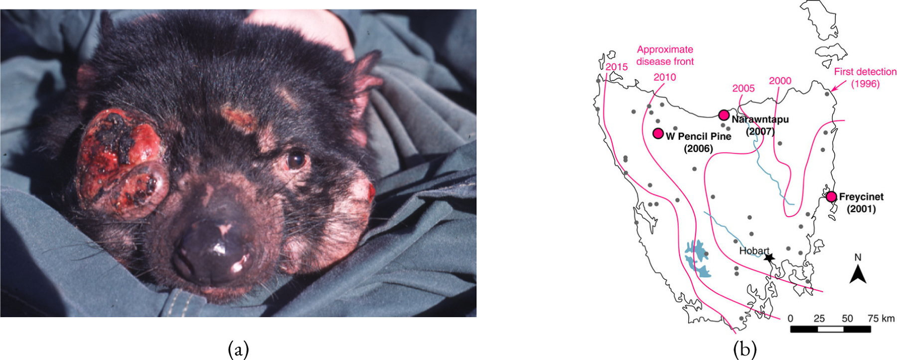
(a) Devil facial tumour disease causes tumours to form in and around the mouth, (Photo: Menna Jones) adapted from McCallum and Jones (2006). (b) Spread of DFTD across Tasmania, adapted from Epstein et al. (2016).
In this paper we consider the effectiveness of bait drop or trap-vaccinate-release wildlife vaccines either as a single intervention or combined with selective culling of only highly diseased animals who are no longer reproducing. We find that successful elimination of the disease is the only way to have long term recovery of the devil population to pre-DFTD numbers. Additionally, we explore the preliminary data evidence that devils may be developing some natural immunity to the disease and how much immunity would need to develop to allow for a sustainable population without human intervention (Hamede et al., 2021).
2. Background
We developed a modified SEIV (Susceptible, Exposed, Infected, Vaccinated) model and calibrated it to the population data presented by Cunningham et al. (2021). Through the parameter estimation process we found that we must split the infected individuals into two classes, the Infected class, and an additional class of highly diseased devils who are no longer successfully reproducing, the Diseased class (Hamilton et al., 2019, 2020). Additionally, we are able to estimate the start of DFTD to be in the year 1993, which is in agreement with other efforts to predict to emergence date of DFTD (Kwon et al., 2020; Cunningham et al., 2021). After successfully parameterizing the model with and without the disease, we examine the population trajectory for the following conditions:
A successful vaccine and bait drop process is developed and implemented.
Highly diseased animals in the Diseased class are culled to remove them from the population.
Devils develop natural resistance to DFTD that slows down movement between Susceptible, Exposed, Infected, and Diseased classes.
None of the above occur.
We found several different successful strategies: bait drop style vaccination programs, the development of high levels of natural immunity, and a conservation program that includes vaccination and the culling of highly diseased animals. However, we find that successful programs are dependent on the length and frequency of the interventions. Our findings are consistent with previous modeling efforts that conclude selective culling alone will not be effective (Beeton and McCallum, 2011) and support models that show vaccine efforts may be the most effective strategy (Bruno et al., 2017; Bobbitt et al., 2020). We find that devils would need to develop at least a 60% natural immunity to DFTD for the disease to have a high probability of elimination. Therefore, our model supports that a vaccine strategy, even if it is not sufficient to eliminate the disease, may help the devils maintain a sustainable population while such natural immunity may be developing.
3. Model Description
We developed a stochastic model whose diagram is shown in Figure 2. Equations (1)–(5) describe the base population model without any disease. Adult devils produce juvenile devils at a rate and juvenile devils become adult devils at a rate . Juveniles and adults have non-disease death rates of and , respectively, as well as a combined death rate due to overcrowding of . The rate parameters in Equations (1)–(5) were fit to data from Cunningham et al. (2021) assuming our estimated carrying capacity of 61322 devils for the whole ecosystem.
Figure 2:
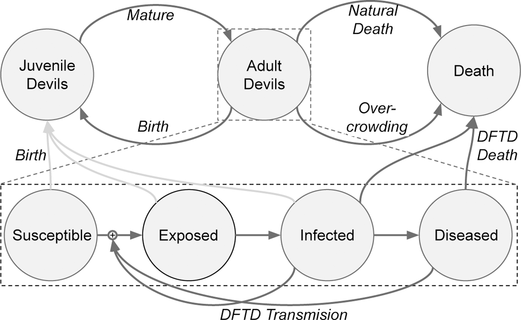
Diagram of our model. We sub-divide “Adult Devil” into four stages of the disease: Susceptible (devils without DFTD), Exposed (Devils who have been exposed to, but are not spreading DFTD), Infected (Devil who are spreading DFTD), and Diseased (Devils who are spreading DFTD and are heavily impacted by it). Note, we assume that Diseased devils do not reproduce.
| (1) |
| (2) |
| (3) |
| (4) |
| (5) |
To model the disease we sub-divide “Adult Devil” into four stages of the disease: Susceptible (devils without DFTD), Exposed (Devils who have been exposed to, but are not spreading DFTD), Infected (Devil who are spreading DFTD), and Diseased (Devils who are spreading DFTD and are heavily impacted by it), as shown in Equations (6)–(11). Note, we assume that Diseased devils do not successfully reproduce due to their advanced diseased state. When Susceptible devils interact with either Infected or Diseased devils, the outcome is Exposed and Infected or Diseased devils respectively at rates and . Exposed devils move to the Infected class after the incubation period at a rate and similarly Infected devils move to the Diseased after the disease progresses at a rate . Infected Devils die at a rate and Diseased Devils at rate .
| (6) |
| (7) |
| (8) |
| (9) |
| (10) |
| (11) |
The model described by Equations (1)–(11) were fit to data presented by Cunningham et al. (2021) and were chosen based on error minimization, visual fit of the model, and consistency with field data on the disease. Figure 3(a) shows the reported total population data as well as our fitted model, extrapolating the devil population if DFTD had not existed. Figure 3(b) shows the reported total population and our fitted total population with DFTD as well as the sub-classes of devils in the model. Table 1 shows average value for the fitted parameter values for the disease. The average time from first exposure to the disease to death from the disease is approximately 24 months. Devils may die from other causes before this two years. While total time from exposure to death may be shorter in individual devils, we are choosing these parameters that are both biologically feasible and fit the Cunningham (Cunningham et al., 2021) data as best as possible.
Figure 3:
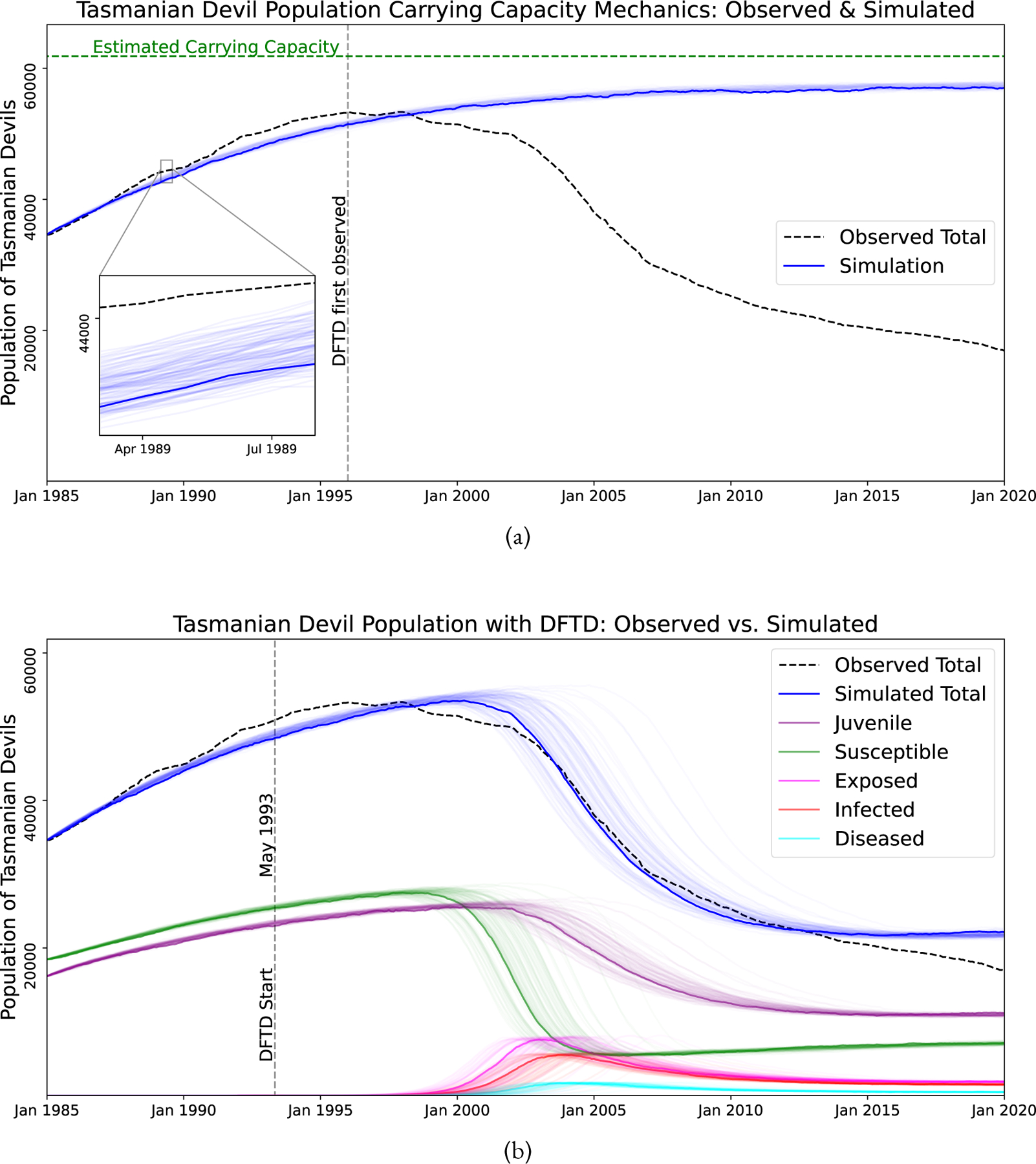
Simulations of 100 stochastic trajectories of the Tasmanian Devil population model. The first trajectory is dark, while the rest are lighter. The dashed black line represents observed Tasmanian Devil populations (Cunningham et al., 2021). (a) Simulation of the model had DFTD not existed: simulated total population (blue lines) and observed (dashed black line). (b) Simulation of model with DFTD: simulated total population (blue lines), simulated sub-groups (colored lines), and observed (dashed black line).
Table 1:
Model Parameters.
| Parameter | Value | Units | Notes |
|---|---|---|---|
| Initial juvenile population | 16165 | Devils | |
| Initial adult population | 18450 | Devils | |
| 0.055 | Devils−1months−1 | ||
| 0.04 | Devils−1months−1 | ||
| 0.007 | Devils−1months−1 | ||
| 0.02335 | Devils−1months−1 | Susceptible and Exposed | |
| 2.3e-07 | Devils−2months−1 | ||
| 1.0e-05 | Devils−1months−1 | ||
| 3.84e-05 | Devils−1months−1 | ||
| 10.25 | months Devils | ||
| 10.74 | months Devils | ||
| 0.022609 | Devils−1 months−1 | ||
| 0.29017 | Devils−1 months−1 | ||
| DFTD start | 100 | months | May 1993 |
4. Conservation Intervention Strategies
We consider how a vaccine campaign, a culling campaign, or a combination of both could impact long term devil populations. We aim to find a parameter space that eliminates DFTD and allows devil populations recover to their pre-DFTD populations. Additionally, we explore how much natural immunity in what time frame would be needed for devils to sustain their population without human intervention. We show how a vaccine campaign may allow maintenance of a sustainable population while devils develop natural immunity even if the vaccine campaign is not sufficient to eliminate the disease. First we model devil populations if no interventions are present as comparison.
4.1. No intervention
If no intervention is done, we see in Figure 4 that the model predicts that DFTD will become endemic and devils will maintain a population of roughly one third of their peak population. We do note Figure 4 shows juvenile devils as the largest class of devils in the endemic phase. This is troubling because juvenile devils are the most susceptible to death due to external influences such as from vehicle strikes and domestic dog attacks (Hobday et al., 2008; Jones, 2000). Our model does not account for these potentially higher death rates, therefore it is possible that the long term population would decrease more than the figure shows due to the increased proportion of the population being juveniles.
Figure 4:
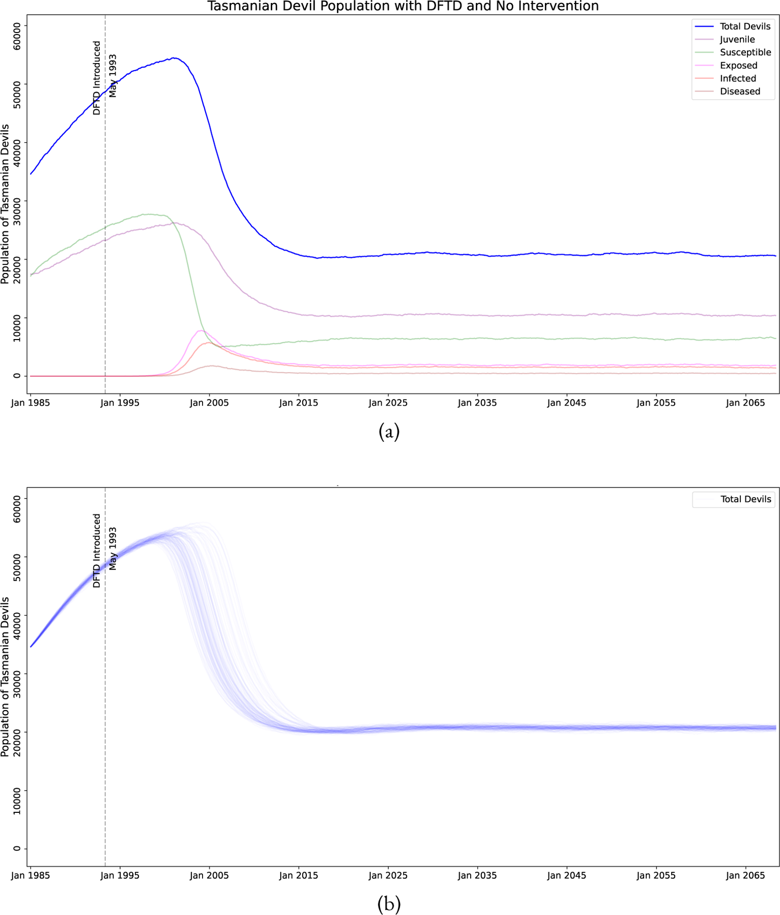
Simulation of the model with no interventions, for comparison. Note that with no human intervention DFTD become endemic and the population of devils reaches a steady-state. Also note, however, that the population of juvenile devils is larger than adult devils in this state. (a) A single stochastic trajectory, showing all the sub-classes. (b) 100 stochastic trajectories, showing only total devil population.
4.2. Evolved natural immunity
It has been hypothesized that the devils are becoming naturally immune through strong evolutionary selection pressure (Hamede et al., 2021) with evidence of tumor regression in rare cases (Pye et al., 2016; Wright et al., 2017; Margres et al., 2020). We model this by reducing the transmission rate of the disease by multiplying by 1.0 immunity . For example, if we assume immunity is 60%, this means an individual devil will only contract the disease at 40% the rate it would had the devil no natural immunity. Due to the rarity of tumor regression, we do not model a way for devils to move backwards in the disease classes from Diseased to Infected, Infected to Exposed, or Exposed to Susceptible. This may be modeled in future efforts if more evidence of natural regression or vaccine induced regression is well documented. Figure 5 shows simulations of this program assuming that natural immunity began to develop in January 2022 growing at an exponential rate of 0.0075 to a maximum of 70% immunity. The exponential rates 0.005, 0.0075, 0.01 corresponds to approximately 23, 15, and 11 years for the devil population to gain half of the max level, respectively. We note that if devils naturally develop a high level of immunity to the disease, they may be able to recover on their own without human intervention. We consider how high the immunity must reach for potential disease elimination by considering the maximum immunity level reached as well as when natural immunity started to develop, see Equations (12)–(14) and Table 2 for more details. Figure 6 shows that at only 50% maximum immunity, elimination of DFTD is not possible, but at 70% maximum immunity, the devils may be able to eliminate the disease. There is not sufficient evidence that this level of natural immunity is achievable at all or in what time frame it would take to achieve such a high level of natural immunity.
Figure 5:
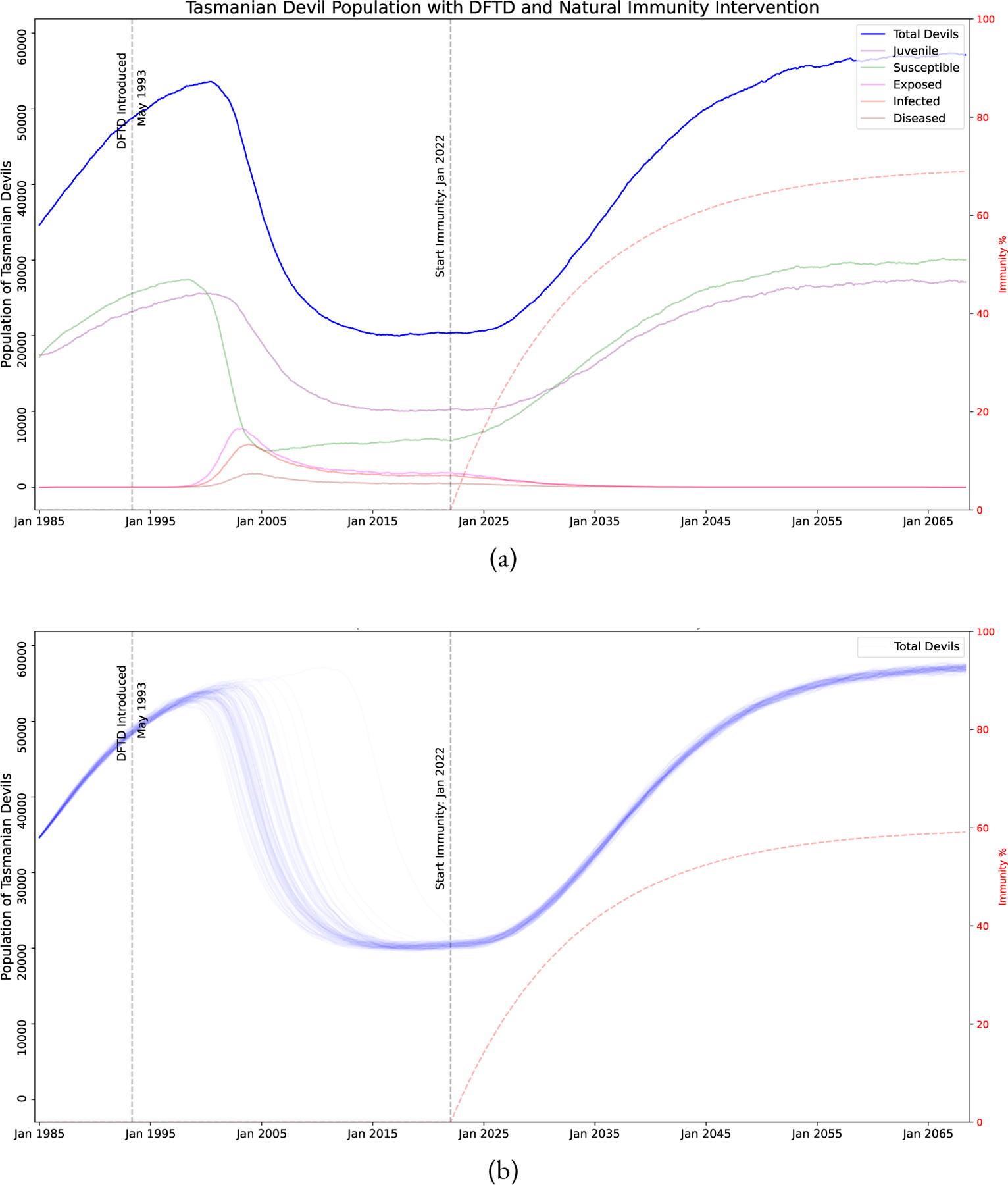
Simulation of DFTD model with naturally evolved immunity. Parameters of the program: starting Jan 2022 at 0% and growing exponentially at a rate of 0.0075 to a maximum of 70%. The time-varying immunity level is indicated by the dashed red line. Even in cases where evolved natural immunity does not eliminate it, DFTD becomes endemic in the devil population and the population trends towards the carrying capacity of the environment with a more sustainable adult devil population (in contrast with the “no intervation” results). (a) A single stochastic trajectory, showing all the sub-classes. (b) 100 stochastic trajectories, showing only total devil population.
Table 2:
Parameters for natural immunity.
| Parameter | Range | Description |
|---|---|---|
| Start | Date when Immunity begins | |
| Growth Rate | Exponential growth rate of immunity | |
| Max Level | Maximum level of immunity |
Figure 6:

Although there is currently no evidence that Tasmanian Devils are or will develop immunity to DFTD, we explored the outcomes if such immunity evolved. Probability of eliminating DFTD with naturally evolved immunity reaching of a maximum level of 50–100% and starting to evolve between 2017 and 2027. Probability of eliminating DFTD with natural immunity, showing immunity max level versus (a) Immunity Start, with immunity growth rate of 0.0075 (15 years to reach the half-maximum immunity level). (b) Immunity Growth Rate, with immunity start as Jan 2022.
| (12) |
| (13) |
| (14) |
4.3. Culling
One possible intervention is culling of devils who are heavily impacted by DFTD (the “Diseased” sub-class in our model, see Equation (15) and Table 3). These are animals that are generally in the last 3 months of life and often die due to the disease. For our analysis, culling indicates the individuals are removed from the general population. The implementation of this intervention in the field could take many forms including a capture and quarantine type program. Figure 7 shows simulations of this program. We note that while there will be small rise in devil populations with a culling program, the disease will quickly return to its current endemic state after the conclusion of a culling program. Additionally, Figure 8 shows a 0% probability of eliminating DFTD using culling strategies alone with a culling program from 3–11 years and culling anywhere from 25% to 75% of the Diseased animals. Therefore, our model supports that culling alone is not a viable long term strategy. Additionally, many remote regions of Tasmania are not accessible via roads, so large-scale culling of diseased devils is not feasible in the foreseeable future.
Table 3:
Parameters for culling intervention.
| Parameter | Range | Description |
|---|---|---|
| Cull Rate Diseased | Rate of culling of Diseased devils | |
| Program Length | Duration in years of the cull program |
Figure 7:
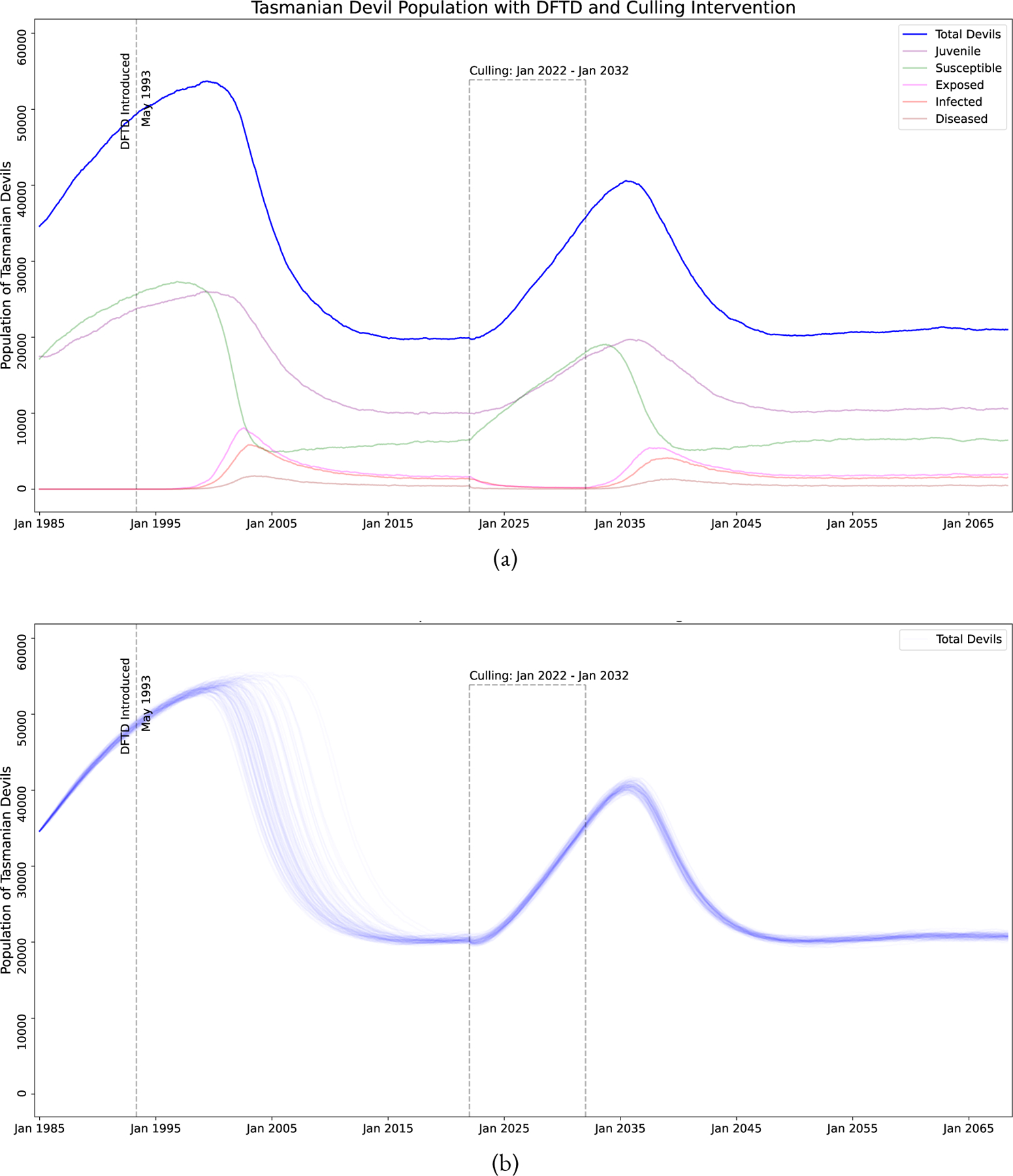
Simulation of DFTD model with a 10 year culling program where 50% of heavily diseased devils removed from the population (Diseased state). (a) A single stochastic trajectory, showing all the sub-classes. (b) 100 stochastic trajectories, showing only total devil population.
Figure 8:
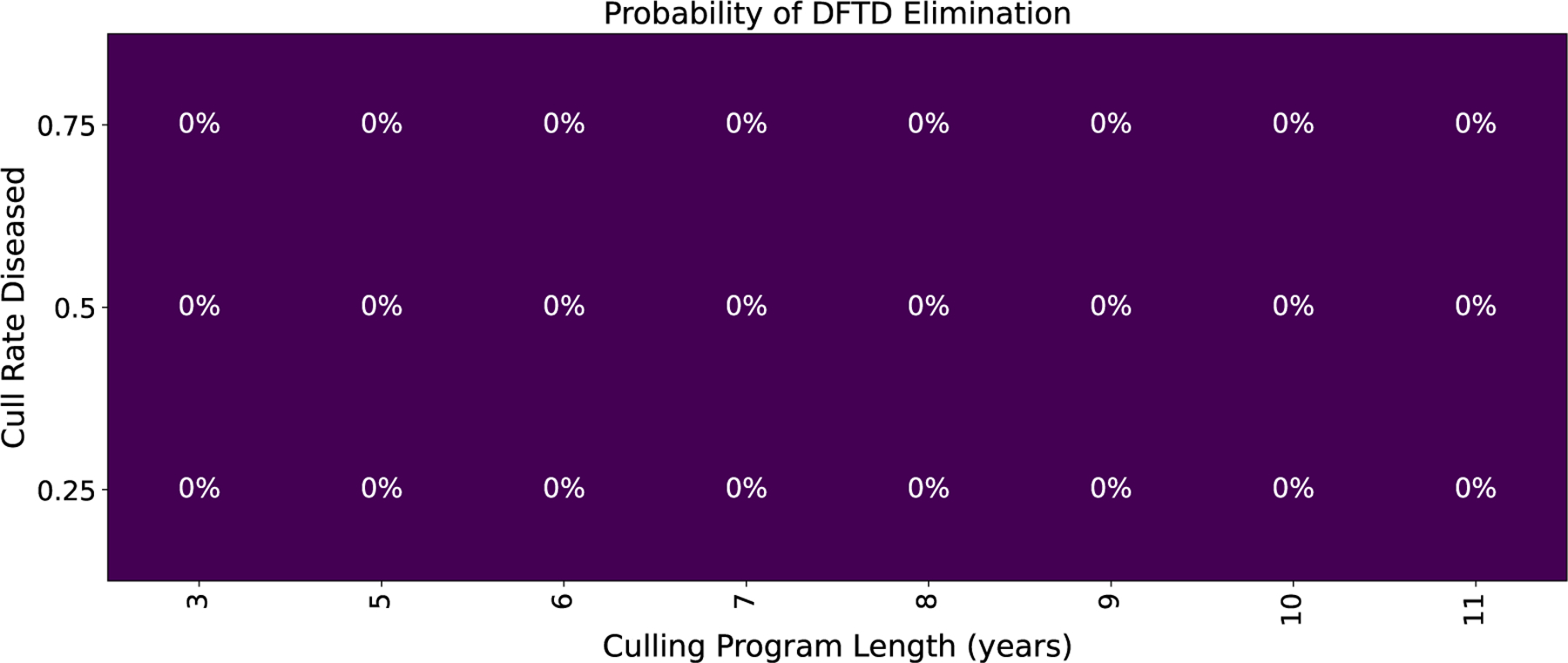
Probability of eliminating DFTD with culling.
| (15) |
4.4. Vaccination
Wildlife vaccination against DFTD is still in development but we consider what efficacy of vaccine is needed to be productive as well as how long and how frequent a vaccine campaign would be needed to allow devil populations to recover (Owen and Siddle, 2019; Tovar et al., 2017; Flies et al., 2020). Figure 9 shows the model diagram with the addition of the Vaccinated state, Equations (12)–(14) and Figure 9 shows the additional interactions, and Table 4 shows the description and ranges of the vaccination parameters. The model considers the vaccination to be administered from 1–12 times per year for 1–10 years with proportion of the devils receiving the vaccine. The vaccine has an efficacy rate of , therefore Vaccinated devils become Exposed devils after interacting with an Infected or Diseased devil at reduced infection rates and respectively.
Figure 9:
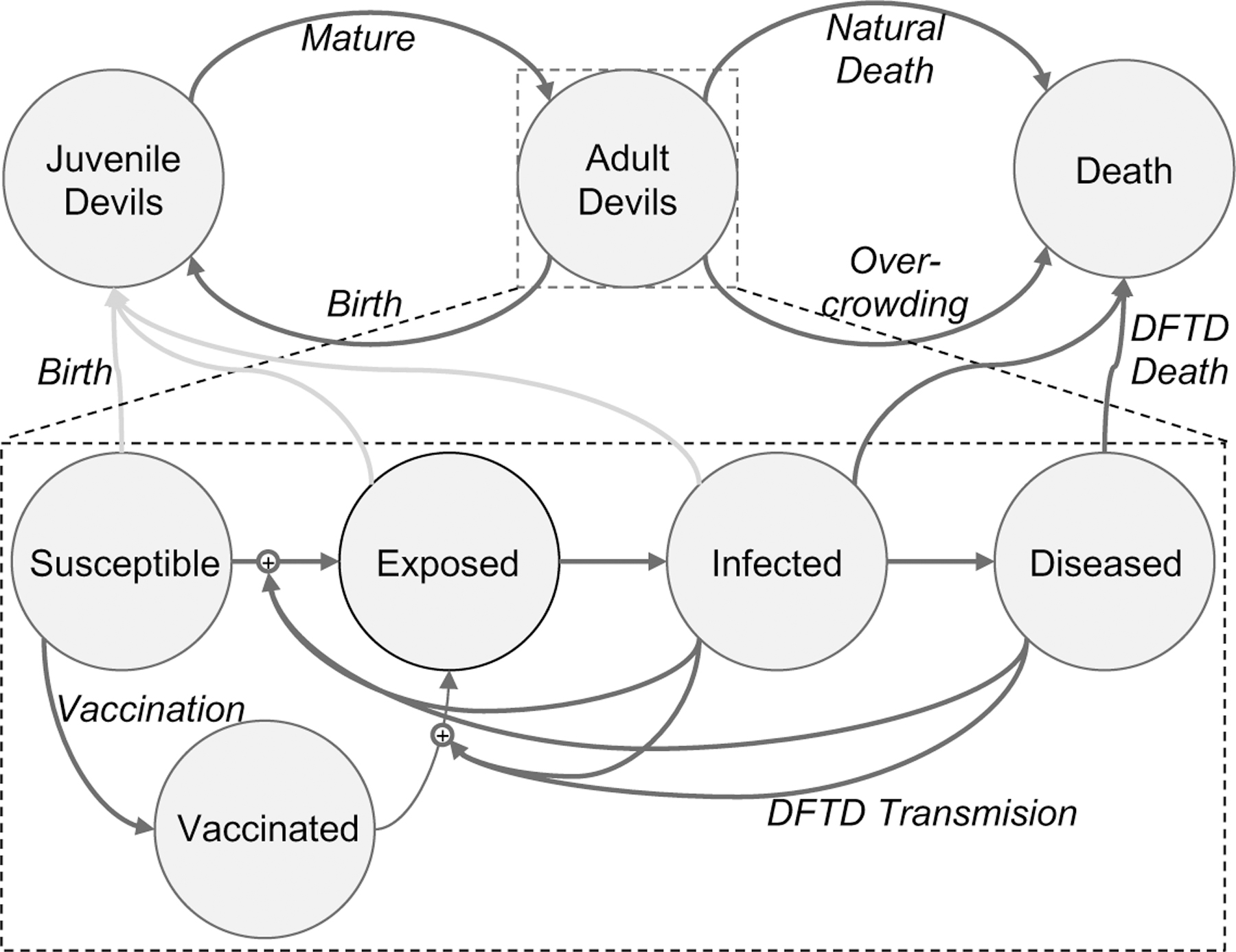
Diagram of our model with the Vaccinated state. We sub-divide “Adult Devil” into five stages of the disease, adding Vaccinated as a subset of the Susceptible population. This state has a lower rate of becoming Exposed given contact with an Infected or Diseased devil.
Table 4:
Parameters for vaccination intervention.
| Parameter | Range | Description |
|---|---|---|
| Fraction of Adult devils vaccinated on each drop | ||
| Probability of vaccine failure | ||
| Program Length | Duration in years of the vaccination program | |
| Program Frequency | Number of vaccination drops per year |
Figure 10 shows the model with a ten year vaccination program implemented. A successful campaign where devil populations increase to pre-DFTD populations post the end of the campaign is shown in Figure 10(a). This successful campaign assumes vaccine with only 40% efficacy (60% failure rate) that is delivered to 80% of the devil population, six times per year. A campaign that temporarily increases devil populations but does not eliminate the disease and the population decreases back to the endemic steady state is shown in Figure 10(b). This campaign assumes the same parameters as the successful campaign but reduces vaccine delivery to only two times per year.
Figure 10:
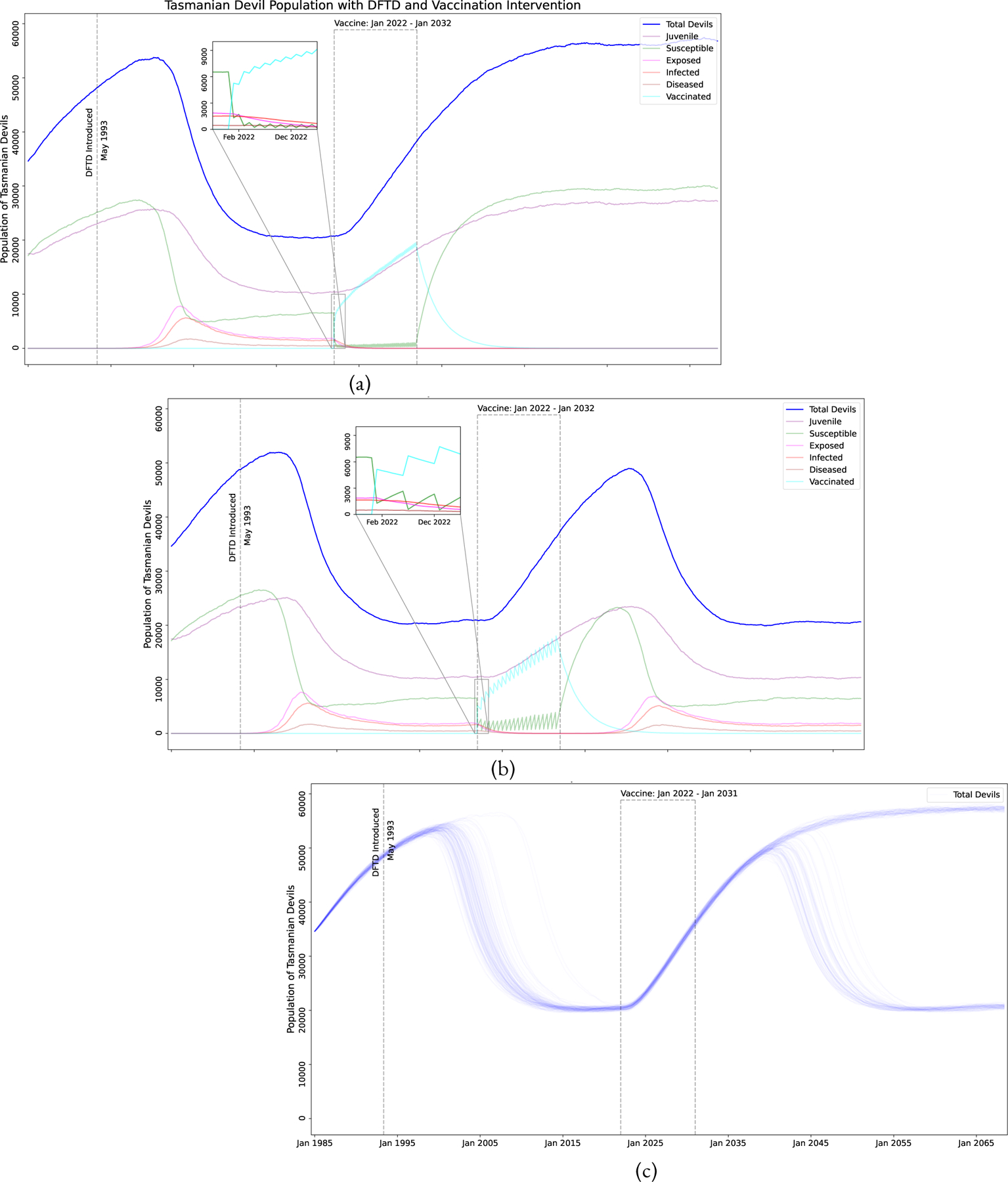
Simulation of DFTD model with a 10 year vaccination program. (a) A program that successfully eliminates DFTD, using the parameters: 60% vaccine failure rate, delivered to 80% of the population 6 times a year. The inset shows the vaccination events, and resulting spikes in the population of Vaccinated and Susceptibilities. (b) A program that temporarily increases devil populations but does not eliminate DFTD, using the parameters: 60% vaccine failure rate, delivered to 80% of the population 2 times a year. The inset shows the vaccination events with a different frequency. (c) A plot of 100 stochastic trajectories, showing approximately 50% DFTD elimination. Simulations used the parameters: 40% vaccine failure rate, delivered to 80% of the population 4 times a year for 9 years. This shows how we calculate the percentage effectiveness of a conservation strategy of a specific parameter set, by counting the number of stochastic trajectories where DFTD is eliminated (blue lines ending near the carrying capacity) divided by the total number of trajectories simulated.
We note that due to the high transmissibility of DFTD, if the disease is not successfully eliminated, a single diseased animal will eventually push the population back into the current endemic state if no other interventions or acquired immunity develops. Therefore we consider the probability of DFTD elimination based on the vaccine program length in years versus the vaccine frequency per year, the proportion of devils who are vaccinated and the vaccine failure rate (1-vaccine efficacy). Figure 11 shows that in all cases, a program length of at least eight years is needed for at least a 50% probability of DFTD elimination. In Figure 11(a) we assume a low vaccine failure rate of only 10% with 80% of the devils receiving the vaccine. We notice that a vaccine frequency of at least four to six times per year is needed to achieve over a 50% probability of disease elimination. In Figure 11(b) we also assume a low vaccine failure rate of only 10% with a frequency of four times per year. We note that developing baits that allow the vaccine to be delivered to a higher proportion of the devils is imperative and the more successful the bait drops are, the fewer years the vaccine campaign can be for potential successful DFTD elimination. Finally in Figure 11(c) we see something interesting about the vaccine failure rate. We note that the probability of disease elimination does not vary greatly in each column, indicating that vaccine failure rate does not play a strong role in disease elimination. A 10% failure rate (bottom row) does not lead to much greater elimination probabilities than a 60% failure rate (top row) with the same length of the vaccine campaign. Therefore our model supports that with with the development of almost any vaccine, efforts put into successful baits in a long term, frequent vaccine campaign can have a high probability of eliminating DFTD.
Figure 11:
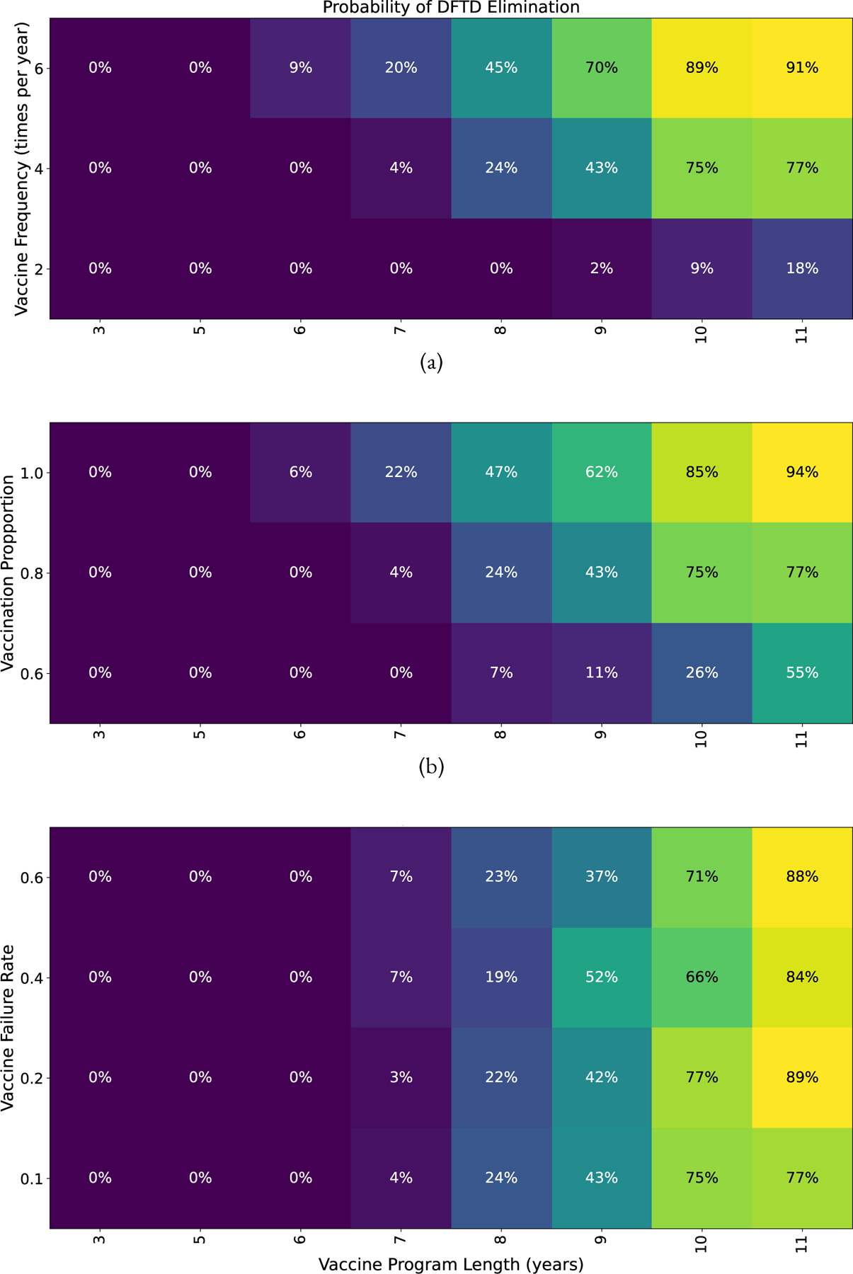
Probability of eliminating DFTD with program length between 3 and 11 years versus (a) Vaccine frequency (number of times per year) while fixing vaccine failure rate at 0.1, and vaccination proportion at 0.8. (b) Vaccination proportion while fixing vaccine failure rate at 0.1 and vaccine frequency of 4 times a year. (c) Vaccine failure rate while fixing vaccination proportion 0.8 and vaccine frequency 4 times a year.
| (16) |
| (17) |
| (18) |
Note, that we implement the vaccination process in Equation (16) as single event. This mimics the implementation of the proposed bait drop vaccination strategies. Thus our vaccination program has four parameters (as shown in Table 4): is the fraction of all wild Tasmanian devil that will be vaccinated by a single drop, “Program Length” is the number of years the conservation will be implemented, and “Program Frequency” is the number of times per year that bait drops will be performed. We assume a bait drop is an environment wide distribution of vaccine within a short time period (modeled as instantaneous).
4.5. Vaccination and culling combined
A vaccination campaign can be costly and time consuming, therefore we consider if selective culling of highly diseased animals can reduce the length of a potential vaccine campaign. Animals considered for culling are in the Diseased sub-class meaning they are in the late stages of DFTD, have noticeable visible tumors, and are in the last 3–4 months of their life. While these devils are assumed to not be successfully mating, it is still possible for them to spread the disease to Susceptible devils. Figure 12 shows the effect on the devil population of a program that includes both vaccination and culling. Figure 13 shows that vaccination and culling are more successful than either conservation strategy alone.
Figure 12:
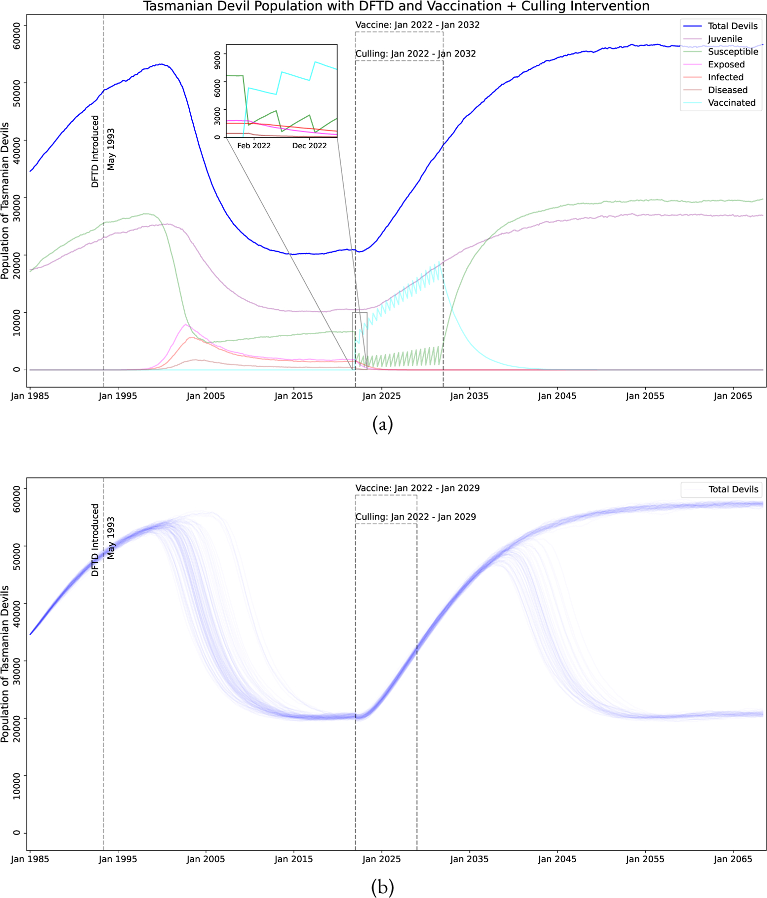
Simulation of DFTD model with both vaccination and culling. (a) Culling and Vaccination program lengths of 10 years, vaccine failure rate of 0.6, vaccination proportion of 0.8, vaccine frequency of 2 times a year, and a cull rate of 0.5. (b) Culling and Vaccination program lengths of 7 years, vaccine failure rate of 0.4, vaccination proportion of 0.8, vaccine frequency of 4 times a year, and a cull rate of 0.5.
Figure 13:
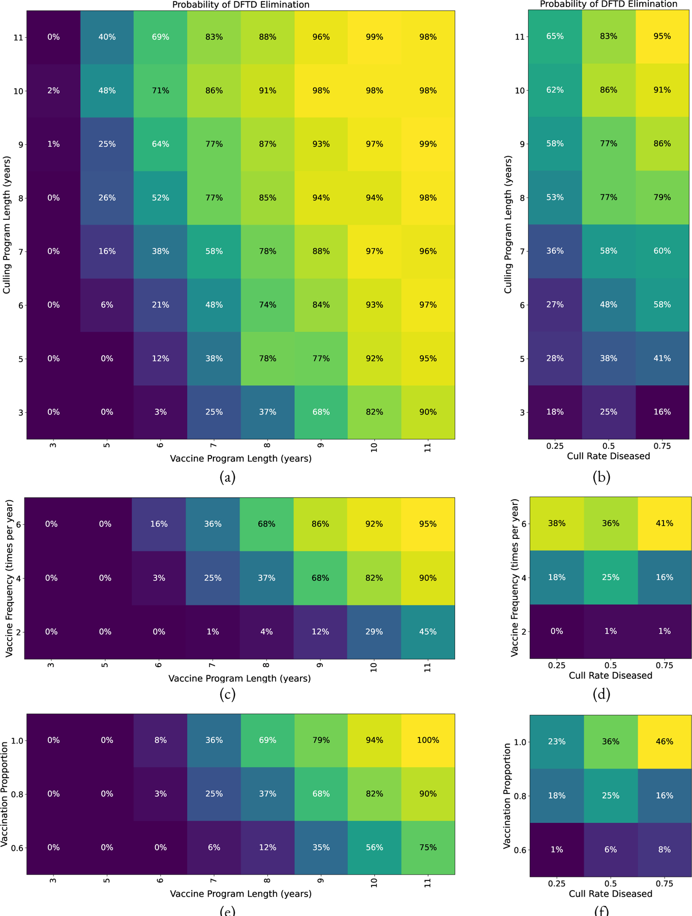
Probability of eliminating DFTD with both vaccination and culling. Parameters held constant (unless specified by the axes) are: vaccine failure rate of 0.4, vaccination proportion of 0.8, vaccination and culling program length of 7 years, vaccine frequency is 4 times a year, and Diseased devil culling rate of 0.5. (a) Culling Program length versus Vaccination Program length. (b) Culling Program length versus Diseased devil culling rate. (c) Vaccine Frequency versus Vaccine Program Length. (d) Vaccine Frequency versus Diseased devil culling rate. (e) Vaccine Proportion versus Vaccine Program Length. (f) Vaccine Proportion versus Diseased devil culling rate.
5. Conclusion
In developing a model parameterized based on 35 years of devil data and 25 years of disease data (Cunningham et al., 2021), we are able to show the potential for DFTD interventions to successfully eliminate the disease. While there is limited evidence that devils are developing natural immunity to the disease, elimination of the disease and population recovery can be supported by a multi-year vaccine campaign, potentially combined with selective culling of highly diseased animals. Our model supports that the devils are currently in the endemic phase and may stay at their current population levels, but with potential changes to the age structure of the population, current devil populations may not be sustainable. A devil population of primarily juveniles, as our model shows the population will become, is problematic and unlikely to lead to a long term healthy population. Therefore, lacking strong evidence for the development of a high level of natural immunity, our model supports vaccine intervention when a viable vaccine become available.
Our simulation results can be interpreted to make a few conclusions. Parameter sweeps of different vaccination strategies show that the results are less sensitive to vaccine failure rate, i.e. decreasing vaccine failure rate does not necessarily increase elimination probability (Figure 11c). Our results show that focusing on vaccine distribution by increasing vaccination frequency and vaccination proportion show increasing chance of elimination (Figures 11a and 11b). However, for a vaccination program alone results will likely take at least 9 years (results in Figure 11). The timeline for DFTD eradication can be accelerated by combining a vaccination program with a culling program, with possible elimination in 7 years (results in Figure 13a). It may be beneficial to the long term health of the Tasmanian Devil population to explore some of these options.
While our model shows vaccination as the most effective way to eliminate DFTD, vaccine production and distribution cost could be a major barrier to widespread devil vaccination. Technological advances continue to streamline large-scale vaccine production, but the cost to produce the viral vector-based vaccines will remain significant. Strategies that allow lower doses of vaccine to be used in each bait could decrease cost proportionally to dose reduction. For example, a single-cycle adenoviral vector that copies its genome in host cells but cannot make new viruses could decrease dosage by up to three orders of magnitude per vaccine (Barry, 2018).
The frequency and density of bait distribution will likely be the primary determinant of cost. Previous rabies oral bait vaccine analysis suggests that high bait density of 300 baits/km2 could be needed for skunks (Mephitis mephitis) whereas 75 baits/km2 could be effective for raccoons (Johnson et al., 2021). However, two reviews of global oral rabies vaccination years of rabies baiting suggest that bait densities of less than 20 baits/km2 can eradicate rabies (Müller et al., 2015; Maki et al., 2017). It is currently unknown how many baits/km2 would be needed to effectively vaccinate the devil population. A density of 20 baits/km2 across the island of Tasmania (68,000 km2) would require 1,360,000 for a single full scale baiting operation. Alternative approaches that focus on regional elimination of DFTD and establishing buffer zones with high devil density as the population recovers would reduce cost. Another innovative approach would be to engage land owners and other community members to assist in vaccine distribution and monitoring (Duamor et al., 2022). Finally, the vaccine could amplify any natural resilience to DFTD that evolves in the population, thus potentially decreasing the frequency and duration of bait vaccine campaigns. Local, national, and international community support for this Tasmanian icon remains staunch, suggesting that cost of mass vaccination campaigns may be surmountable if an effective vaccine can be developed.
6. Methods
Our simulations were performed using the software package GillesPy2 (Drawert et al., 2019) version 1.6.9. GillesPy2 is a complete rewrite from the original (Abel et al., 2016). GillesPy2 is part of the StochSS (Drawert et al., 2016) suite of software (Drawert et al., 2018; Jiang et al., 2021). Our simulation methodology was of discrete stochastic simulation, of the style of the Stochastic Simulation Algorithm (SSA) (Gillespie, 1976, 1977) (sometimes known as the Gillespie method). Specifically, we use the Tau-Hybrid solver with events, which utilizes the Tau-Leaping (Gillespie, 2001) method to simulate the stochastic reaction system.
StochSS is an online, open interface designed for non-technical audiences to create models (differential equation, stochastic, biological, epidemiological, and more) and analyze results utilizing built-in methods for producing time-series graphs and parameter sweeps along with an extensible jupyter notebook interface for more advanced users. StochSS can be used simply and immediately online through our web interface, StochSS Live! live.stochss.org, or users can create their own StochSS environment either locally or on their own server. Additionally, while StochSS provides a comprehensive and robust environment for modeling, the underlying packages which power StochSS can all be installed and used individually. StochSS is powered by GillesPy2, a modeling tool kit for single well-mixed volumes providing a wide range of ODE and stochastic simulation techniques, SpatialPy a modeling system that couples reaction-based networks with particle-based fluid dynamics, and Sciope(Singh et al., 2020), a toolkit for model exploration and parameter inference. All three are Python 3 packages, available through PyPi and accessible through simple pip installations.
Users can log in to the StochSS Live! platform at https://live.stochss.org using a Google account through Google OAuthID services to begin using the platform for this scientific research. Once logged in, users can begin by creating a model, or via uploading a previously constructed model. The StochSS Live! interface also provides a tutorial to assist users in getting started with model building and simulation.
To create a model in StochSS or GillesPy2, first you must identify which quantities of interest are time changing. In our model, these quantities are the total number of devils, and each sub-category of the devil population, these are known as the “variables” (in StochSS) or “species” (in GillesPy2). Next, we identify the constant values that identify the rates of changes of the quantities (e.g. maturity rate, death rate), these are known as “parameters." Finally, we need to identify the interactions which cause changes to the variables, and what is consumed and produced by that interaction. These are known as “reactions.” For example, the maturity reaction, Equation (2), consumes one juvenile devil and produces one adult devil at the rate . Once all the species, parameters and reactions have been identified, and a time span of the simulation has been specified, then the model can be simulated and the results plotted. In our model we use “month” as our output interval of our time span, starting at January 1985 ending either at January 2020 or May 2068 (1000 months). See the next section for more details on how to recreate our models.
6.1. How to reproduce this work
The modeling, simulation, and analyses were all done with StochSS (Jiang et al., 2021). One powerful feature of the StochSS Live! web platform is the ability to publish models and projects, and to create publicly accessible links that will allow other users to download these to their own account on StochSS Live!. This enables researchers to make their work easy to review and reproduce, furthering collaboration and peer-review. To reproduces this work, click this link: https://open.stochss.org/?open=https://github.com/StochSS/devils_dftd_modeling/raw/main/SavingTheDevilsIsInTheDetails.zip.
We have created a “StochSS project” that contains all the models, simulation, data, and analysis workflows that were used to create the results in this paper. Clicking the link above will open the users’ web browser to their copy of this project in their account on the StochSS Live! web platform. If a user is not signed in, they will be prompted to login using a Google OAuthID (e.g. any Gmail account, or Google organization account). Once logged in, the user will see a loading screen while the project is transferred from its hosting (ours is on GitHub), and uploaded into their account. When the transfer is complete, the project will open automatically and the user will see a listing of models and their associated workflows, which are embedded in Jupyter Notebooks (Kluyver et al., 2016). The user can then click on the “1-Devils-Parameter_Fitting” model, this will show the variables (Devils, Juvenile, Adult), Parameters, and Reactions of the model. If the users then clicks “Simulate” (lower right) then “Preview.” They will see a plot of the population of the Tasmanian devils over time (units of months since January 1985), if DFTD had not been introduced to the population. If the users goes back to the project’s model listing and clicks on “2-Devils_DFTD-Parameter_Fitting” model, they can and see the population of Tasmanian Devils with DFTD introduction. All simulation figures in this paper were generated with the notebooks contained in this project. From the project listing, click on “Devils-Parameter_Fitting” (below the “1-Devils-Parameter_Fitting” under the “Workflows” tab). This will open that notebook in a new tab. Figure 3(a) and Figure 14(a) were created with this notebook. For the reproduction of all other figures, see the “Notes” tab under each model for details. Please note, some of the workflows in these notebooks are very computationally intensive, especially the parameter sweep workflows for Figures 6, 8, 11, 13, and 14. In addition, all of our code is posted on GitHub at: https://github.com/StochSS/devils_dftd_modeling.
Figure 14:
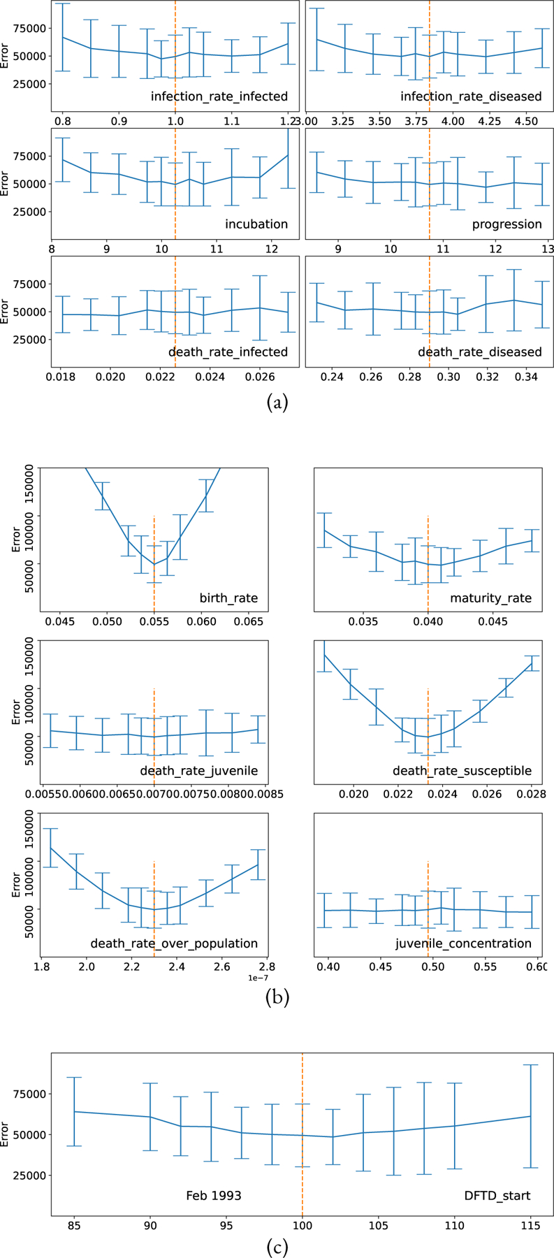
Parameter Space Exploration, plots show the error (L2 norm distance metric) between simulated trajectories and data. Vertical dashed line show selected model parameters (see Table 1). Each parameter point was simulated with 1000 stochastic trajectories, the distance to the observed data was calculated for each of trajectories, the mean and standard deviation of that data is shown in the figure. (a) Parameter fitting for Devils without DFTD. (b) Parameter fitting for Devils with DFTD. (c) Parameter fitting for the start date of DFTD.
6.2. Model parameterization
We found our set of parameters (see Table 1) using a combination of expert knowledge and a computational technique, similar to the method outlined in (Singh et al., 2020). See Figure 14 for plots showing the sensitivity of the parameter space near the parameter points shown in Table 1.
Due to the stochastic nature of this model, exact parameter fitting is challenging. Our process is as follows. At each candidate point in parameter space, 1000 stochastic trajectories were simulated. For each trajectory, the error was calculated by taking the L2 norm of the difference between the “Total Devils” variable and the time-series data of the wild devil population from (Cunningham et al., 2021). The mean and standard deviation of the distances is shown in the error bar plot. For each candidate point in parameter space, we used this process to compute the local slope of error by calculating the error distribution for candidate points that are slightly higher and slightly lower in value for each of the eleven parameters in our model. We looked for nearby candidate points that had a lower average error, and repeated this process until we found a local minima candidate point that recapitulated the devil population effectively. Our parameter space was constrained using non-DFTD carrying capacity of the environment (Figure 3a) and the average time from exposure to death of a devil is close to 24 months (McCallum et al., 2007). See the parameter exploration notebooks in the StochSS Project: “Devils-Parameter_Fitting” and “Devils_DFTD-Parameter_Fitting” to review and reproduce this procedure.
Acknowledgments
We acknowledge funding from NIBIB Award 2-R01-EB014877-04A1. No official position or official endorsement should be inferred.
References
- Abel JH, Drawert B, Hellander A, and Petzold LR (2016). GillesPy: a python package for stochastic model building and simulation. IEEE life sciences letters 2(3), 35–38. 136 [DOI] [PMC free article] [PubMed] [Google Scholar]
- Barry M (2018). Single-cycle adenovirus vectors in the current vaccine landscape. Expert Review of Vaccines 17 (2), 163–173. 136 [DOI] [PMC free article] [PubMed] [Google Scholar]
- Beeton N and McCallum H (2011, dec). Models predict that culling is not a feasible strategy to prevent extinction of Tasmanian devils from facial tumour disease. Journal of Applied Ecology 48(6), 1315–1323. 121, 122 [Google Scholar]
- Bobbitt Z, Comar T, Powell MO, Roberts C, and Schneider N (2020). Impulse vaccination model for the control of devil facial tumor disease impulse vaccination model for the control of devil facial tumor disease. Spora 6(1), 61–71. 122 [Google Scholar]
- Bruno CD, Comar T, Powell MO, and Tameklo A (2017). Age-structured and vaccination models of devil facial tumor disease. SPORA: A Journal of Biomathematics 3(1). 122 [Google Scholar]
- Cunningham CX, Comte S, McCallum H, Hamilton DG, Hamede R, Storfer A, Hollings T, Ruiz-Aravena M, Kerlin DH, Brook BW, Hocking G, and Jones ME (2021). Quantifying 25 years of disease-caused declines in Tasmanian devil populations: host density drives spatial pathogen spread. Ecology Letters 24(5), 958–969. 121, 122, 123, 124, 131, 137 [DOI] [PMC free article] [PubMed] [Google Scholar]
- Dempsey S, Pye RJ, Gilbert AT, Fountain-Jones NM, Moffat JM, Benson-Amram S, Smyser TJ, and Flies AS (2022). Evaluation of oral baits and distribution methods for Tasmanian devils (Sarcophilus harrisii). bioRxiv 121
- Drawert B, Hellander A, Bales B, Banerjee D, Bellesia G, Daigle BJ Jr, Douglas G, Gu M, Gupta A, Hellander S, et al. (2016). Stochastic simulation service: bridging the gap between the computational expert and the biologist. PLoS computational biology 12(12), e1005220. 136 [DOI] [PMC free article] [PubMed] [Google Scholar]
- Drawert B, Hellander A, Petzold L, et al. (2018, Oct). StochSS suite of software https://github.com/StochSS/. 136
- Drawert B, Matthew S, Rumsey B, and Sanft K (2019, March). GillesPy2: python package for stochastic simulation of biochemical systems https://github.com/StochSS/GillesPy2. 136
- Duamor CT, Hampson K, Lankester F, Lugelo A, Mpolya E, Kreppel K, Cleaveland S, and Wyke S (2022). Development, feasibility and potential effectiveness of community-based continuous mass dog vaccination delivery strategies: lessons for optimization and replication. bioRxiv 136 [DOI] [PMC free article] [PubMed]
- Epstein B, Jones M, Hamede R, Hendricks S, McCallum H, Murchison EP, Schönfeld B, Wiench C, Hohenlohe P, and Storfer A (2016). Rapid evolutionary response to a transmissible cancer in Tasmanian devils. Nature communications 7 (1), 1–7. 122 [DOI] [PMC free article] [PubMed] [Google Scholar]
- Fancourt BA, Hawkins CE, Cameron EZ, Jones ME, and Nicol SC (2015). Devil declines and catastrophic cascades: Is mesopredator release of feral cats inhibiting recovery of the eastern quoll? PLoS ONE 10(3), 1–26. 121 [DOI] [PMC free article] [PubMed] [Google Scholar]
- Flies AS, Flies EJ, Fox S, Gilbert A, Johnson SR, Liu GS, Lyons AB, Patchett AL, Pemberton D, and Pye RJ (2020). An oral bait vaccination approach for the Tasmanian devil facial tumor diseases. Expert Review of Vaccines 19(1), 1–10. 121, 128 [DOI] [PubMed] [Google Scholar]
- Gillespie DT (1976). A general method for numerically simulating the stochastic time evolution of coupled chemical reactions. Journal of computational physics 22(4), 403–434. 136 [Google Scholar]
- Gillespie DT (1977). Exact stochastic simulation of coupled chemical reactions. The journal of physical chemistry 81(25), 2340–2361. 136 [Google Scholar]
- Gillespie DT (2001). Approximate accelerated stochastic simulation of chemically reacting systems. The Journal of chemical physics 115(4), 1716–1733. 136 [Google Scholar]
- Hamede R, Madsen T, Mccallum H, Storfer A, Hohenlohe PA, Siddle H, Kaufman J, Giraudeau M, Jones M, Thomas F, and Ujvari B (2021). Darwin, the devil, and the management of transmissible cancers. Conserv. Biol 35, 748–751. 121, 125 [DOI] [PMC free article] [PubMed] [Google Scholar]
- Hamilton D, Jones M, Cameron E, Kerlin D, McCallum H, Storfer A, Hohenlohe P, and Hamede R (2020). Infectious disease and sickness behaviour: tumour progression affects interaction patterns and social network structure in wild Tasmanian devils. Proc. R. Soc. B Biol. Sci 287. 122 [DOI] [PMC free article] [PubMed] [Google Scholar]
- Hamilton DG, Jones ME, Cameron EZ, Mccallum H, Storfer A, Hohenlohe PA, and Hamede RK (2019). Rate of intersexual interactions affects injury likelihood in Tasmanian devil contact networks. Behavioral Ecology 30(4), 1087–1095. 122 [Google Scholar]
- Hobday AJ, Scientific TC, and Minstrell ML (2008). Distribution and abundance of roadkill on Tasmanian highways: Human management options. Wildlife Research 35(January), 712–726. 125 [Google Scholar]
- Hohenlohe PA (2017). Infection of the fittest: devil facial tumour disease has greatest effect on individuals with highest reproductive output pp. 770–778. 121 [DOI] [PMC free article] [PubMed]
- Hohenlohe PA, McCallum HI, Jones ME, Lawrance MF, Hamede RK, and Storfer A (2019). Conserving adaptive potential: lessons from Tasmanian devils and their transmissible cancer. Conservation Genetics 20(1), 81–87. 121 [DOI] [PMC free article] [PubMed] [Google Scholar]
- Hollings T, Jones M, Mooney N, and Mccallum H (2014). Trophic cascades following the disease-induced decline of an apex predator, the Tasmanian devil. Conservation Biology 28(1), 63–75. 121 [DOI] [PubMed] [Google Scholar]
- Hollings T, Jones M, Mooney N, and McCallum H (2016). Disease-induced decline of an apex predator drives invasive dominated states and threatens biodiversity. Ecology 97 (2), 394–405. 121 [DOI] [PubMed] [Google Scholar]
- Jiang R, Jacob B, Geiger M, Matthew S, Rumsey B, Singh P, Wrede F, Yi T-M, Drawert B, Hellander A, and Petzold L (2021, January). Epidemiological modeling in StochSS Live! Bioinformatics 37 (17), 2787–2788. 136 [DOI] [PMC free article] [PubMed] [Google Scholar]
- Johnson SR, Slate D, Nelson KM, Davis AJ, Mills SA, Forbes JT, VerCauteren KC, Gilbert AT, and Chipman RB (2021). Serological responses of raccoons and striped skunks to Ontario rabies vaccine bait in West Virginia during 2012–2016. Viruses 13(2), 157. 136 [DOI] [PMC free article] [PubMed] [Google Scholar]
- Jones ME (2000). Road upgrade, road mortality and remedial measures: impacts on a population of eastern quolls and Tasmanian devils. Wildlife Research 27 (3), 289–296. 125 [Google Scholar]
- Kayigwe AN, Darby JM, Lyons AB, Patchett AL, Lisowski L, Liu G-S, and Flies AS (2022). A human adenovirus encoding IFN-γ can transduce Tasmanian devil facial tumour cells and upregulate MHC-I. bioRxiv 121 [DOI] [PubMed]
- Kluyver T, Ragan-Kelley B, Pérez F, Granger B, Bussonnier M, Frederic J, Kelley K, Hamrick J, Grout J, Corlay S, Ivanov P, Avila D, Abdalla S, and Willing C (2016). Jupyter notebooks – a publishing format for reproducible computational workflows. In Loizides F and Schmidt B (Eds.), Positioning and Power in Academic Publishing: Players, Agents and Agendas, pp. 87 – 90. IOS Press. 137 [Google Scholar]
- Kwon YM, Gori K, Park N, Potts N, Swift K, Wang J, Stammnitz MR, Cannell N, Baez-Ortega A, Comte S, et al. (2020). Evolution and lineage dynamics of a transmissible cancer in Tasmanian devils. PLoS biology 18(11), e3000926. 122 [DOI] [PMC free article] [PubMed] [Google Scholar]
- Maki J, Guiot A-L, Aubert M, Brochier B, Cliquet F, Hanlon CA, King R, Oertli EH, Rupprecht CE, Schumacher C, et al. (2017). Oral vaccination of wildlife using a vaccinia–rabies-glycoprotein recombinant virus vaccine (RABORAL V-RG®): a global review. Veterinary research 48(1), 1–26. 136 [DOI] [PMC free article] [PubMed] [Google Scholar]
- Margres MJ, Ruiz-aravena M, Hamede R, Chawla K, Patton AH, Lawrance MF, Fraik AK, Stahlke AR, Davis BW, Ostrander EA, Jones ME, Mccallum H, Paddison PJ, Hohenlohe PA, Hockenbery D, and Storfer A (2020). Spontaneous tumor regression in Tasmanian devils associated with RASL11A activation. Genetics 215, 1143–1152. 121, 125 [DOI] [PMC free article] [PubMed] [Google Scholar]
- McCallum H and Jones M (2006). To lose both would look like carelessness: Tasmanian devil facial tumour disease. PLoS biology 4(10), e342. 122 [DOI] [PMC free article] [PubMed] [Google Scholar]
- McCallum H, Tompkins DM, Jones M, Lachish S, Marvanek S, Lazenby B, Hocking G, Wiersma J, and Hawkins CE (2007, sep). Distribution and impacts of Tasmanian devil facial tumor disease. EcoHealth 4(3), 318–325. 121, 137 [Google Scholar]
- Müller TF, Schröder R, Wysocki P, Mettenleiter TC, and Freuling CM (2015, August). Spatio-temporal use of oral rabies vaccines in fox rabies elimination programmes in Europe. PLOS Neglected Tropical Diseases 9(8), 1–16. 136 [DOI] [PMC free article] [PubMed] [Google Scholar]
- Owen RS and Siddle HV (2019). Devil facial tumours: Towards a vaccine. Immunological Investigations 48(7), 719–736. 121, 128 [DOI] [PubMed] [Google Scholar]
- Pye R, Hamede R, Siddle HV, Caldwell A, Knowles GW, Swift K, Kreiss A, Jones ME, Lyons AB, and Woods GM (2016, oct). Demonstration of immune responses against devil facial tumour disease in wild Tasmanian devils. Biology letters 12(10). 121, 125 [DOI] [PMC free article] [PubMed] [Google Scholar]
- Rout TM, Baker CM, Huxtable S, and Wintle BA (2017). Monitoring, imperfect detection, and risk optimization of a Tasmanian devil insurance population. Conservation Biology 32(2), 267–275. 121 [DOI] [PubMed] [Google Scholar]
- Singh P, Wrede F, and Hellander A (2020, 07). Scalable machine learning-assisted model exploration and inference using Sciope. Bioinformatics 37 (2), 279–281. 136, 137 [DOI] [PMC free article] [PubMed] [Google Scholar]
- Tovar C, Pye RJ, Kreiss A, Cheng Y, Brown GK, Darby J, Malley RC, Siddle HVT, Skjødt K, Kaufman J, Silva A, Morelli AB, Papenfuss AT, Corcoran LM, Murphy JM, Pearse MJ, Belov K, Lyons AB, and Woods GM (2017). Regression of devil facial tumour disease following immunotherapy in immunised Tasmanian devils. Scientific Reports 7 (February), 43827. 121, 128 [DOI] [PMC free article] [PubMed] [Google Scholar]
- Wright B, Willet CE, Hamede R, Jones M, Belov K, and Wade M (2017). Variants in the host genome may inhibit tumour growth in devil facial tumours: evidence from genome-wide association. Sci. Rep 7 (423). 121, 125 [DOI] [PMC free article] [PubMed] [Google Scholar]


