BIANCA‐MS: An optimized tool for automated multiple sclerosis lesion segmentation

Abstract

In this work we present BIANCA‐MS, a novel tool for brain white matter lesion segmentation in multiple sclerosis (MS), able to generalize across both the wide spectrum of MRI acquisition protocols and the heterogeneity of manually labeled data. BIANCA‐MS is based on the original version of BIANCA and implements two innovative elements: a harmonized setting, tested under different MRI protocols, which avoids the need to further tune algorithm parameters to each dataset; and a cleaning step developed to improve consistency in automated and manual segmentations, thus reducing unwanted variability in output segmentations and validation data. BIANCA‐MS was tested on three datasets, acquired with different MRI protocols. First, we compared BIANCA‐MS to other widely used tools. Second, we tested how BIANCA‐MS performs in separate datasets. Finally, we evaluated BIANCA‐MS performance on a pooled dataset where all MRI data were merged. We calculated the overlap using the DICE spatial similarity index (SI) as well as the number of false positive/negative clusters (nFPC/nFNC) in comparison to the manual masks processed with the cleaning step. BIANCA‐MS clearly outperformed other available tools in both high‐ and low‐resolution images and provided comparable performance across different scanning protocols, sets of modalities and image resolutions. BIANCA‐MS performance on the pooled dataset (SI: 0.72 ± 0.25, nFPC: 13 ± 11, nFNC: 4 ± 8) were comparable to those achieved on each individual dataset (median across datasets SI: 0.72 ± 0.28, nFPC: 14 ± 11, nFNC: 4 ± 8). Our findings suggest that BIANCA‐MS is a robust and accurate approach for automated MS lesion segmentation.

BIANCA‐MS is a new tool for multiple sclerosis automated lesion segmentation which harmonizes the optimization procedure across different scanning protocols and implements a cleaning step to reduce the impact of inter‐rater variability and to further refine lesion segmentation. BIANCA‐MS was validated on several datasets with different image characteristics demonstrating its robustness, accuracy and flexibility.

1. INTRODUCTION

Multiple sclerosis (MS) is an inflammatory disease of the central nervous system, characterized by focal areas of inflammation resulting in lesions seen on magnetic resonance imaging (MRI). The identification of these lesions is the fundamental diagnostic step for the demonstration of dissemination in space and time (Thompson et al., 2018) and plays a role in predicting disease course, as lesion number and volume are weakly associated with short and long‐term changes in physical disability (Brownlee et al., 2019; Tintore et al., 2015).

To date, manual segmentation is considered the best approach for segmenting lesions, but this procedure is time consuming and is affected by intra/inter‐rater variability (Zijdenbos et al., 2002), thus limiting its use in large studies (García‐Lorenzo et al., 2013). Against this background, automated tools have been increasingly developed and employed over the last years (Balakrishnan et al., 2021; Danelakis et al., 2018; Kaur et al., 2020; Ma et al., 2022; Shanmuganathan et al., 2020; Zeng et al., 2020). Among automated methods, artificial intelligence (AI) approaches showed higher performance; however, their use in clinical practice is limited for several reasons. First, the majority of AI tools are developed, trained, and validated on a limited amount of data, mostly using a single scanning protocol (Mårtensson et al., 2020). This often leads to algorithm “default” settings that fail to be generalizable when applied to MRI dataset with different acquisition protocols. Thus, to guarantee similar performance on unseen data, a long and complex optimization pipeline needs to be performed to adapt the algorithm's parameters to new MRI scans (Griffanti et al., 2016; Popescu et al., 2012). Data augmentation can be useful as it accounts for a range of differences (e.g., level of resolution, noise and smoothing). However, it is unlikely to be an adequate or sufficient substitute for using real image from different scanners and protocols. Further, it is not the case that data augmentation will always improve generalization as it may introduces data distribution bias (Xu et al., 2020). Another, MS specific, limit consists of the lack of an extensive evaluation of these tools on large datasets of high‐resolution 3D FLAIR images, now considered the most sensitive sequence for the detection of lesions in MS (Bravo et al., 2014; Filippi et al., 2019). Finally, the inter‐rater differences in lesion contouring affects both manual and automated lesion segmentation and it has been shown that it reduces the performance of AI tools even when the same test data, algorithm settings, and architecture are employed (Shwartzman et al., 2019). All these factors are likely to influence algorithm outcomes, thus hampering their implementation in clinical practice. In this respect, recently published tools achieved promising results. However, they showed limited multicenter generalization in segmentation performance (Cerri et al., 2021; Tran et al., 2022; Valcarcel et al., 2018) or needed large amounts of data to achieve optimal results (Zhang et al., 2021).

In 2016, the FSL group developed a machine learning tool (BIANCA) to segment WM hyperintensities (WMH) of presumed vascular origin (Griffanti et al., 2016). Recently, two studies employed BIANCA for MS lesion segmentation on FLAIR images (Duong et al., 2019; Weeda et al., 2019). However, in the latter (which compares several methods, including BIANCA), very few BIANCA settings (n = 18) were tested on a limited amount of MRI data (n = 14) whereas in the former detailed information about the number of MS subjects and the setting employed were not provided. Therefore, the lack of data or an insufficient optimization process may have limited the algorithm's performance.

In this work BIANCA‐MS, a new pipeline to automatically detect MS WM lesions that is based on the original version of BIANCA, is introduced with the aims to:

1. Provide the best parameter setting to be implemented in BIANCA for MS lesion segmentation, irrespective of scanning protocol, magnetic field strength, set of modalities and image resolution; this harmonized setting would avoid the complex and time‐consuming optimization procedures needed for adapting algorithmic parameters to each dataset.

2. Refine the lesion mask by introducing a post‐processing cleaning step.

Once designed, we (i) compared the performance of BIANCA‐MS with other currently available, and widely used, tools for automatic lesion segmentation in MS; (ii) on a multicenter dataset, tested BIANCA‐MS cross‐center generalization by comparing algorithm performance using mixed and site‐specific training and test sets; and (iii) evaluated BIANCA‐MS performance when all the datasets were pooled together. Finally (iv), we evaluated BIANCA‐MS behavior on the MSSEG MICCAI 2016 challenge dataset.

2. MATERIALS AND METHODS

2.1. MRI data

In this study, MRI data from 470 MS subjects were included, belonging to three datasets that were different with respect to scanner manufacturers, magnetic field strengths and MRI acquisition protocols (Table 1). Dataset 1 consisted of 200 scans acquired at the University of Siena on a 1.5 T Philips Gyroscan MRI (Philips Medical Systems, Best, Netherlands); Dataset 2 consisted of 120 scans acquired at the Meyer Hospital on a 3 T Philips Achieva dStream (Philips Medical Systems, Best, Netherlands); Dataset 3 consisted of 150 scans from a multicenter retrospective study, whose scans were collected at many different imaging centers (n = 23) using similar acquisition parameters. Population demographics are depicted in Table 2.

TABLE 1.

Acquisition protocols for each dataset.

	Dataset 1 (n = 200)			Dataset 2 (n = 120)		Dataset 3 (n = 150)
Image	Flair	T1‐W	PD	Flair	T1‐W	PD	T1‐W	T2‐W
Voxel size (mm3)	0.97 × 0.97 × 3	0.97 × 0.97 × 3	0.97 × 0.97 × 3	1 × 0.97 × 0.97	1 × 1 × 1	0.97 × 0.97 × 3	0.97 × 0.97 × 3	0.97 × 0.97 × 3
TR (ms)	9000	35	30	11000	25	2200–3000	550–700	1800–2800
TE1 (ms)	150	10	90	125	4.6	15–50	10–20	30–50
TE2 (ms)	–	–	–	–	–	80–120	–	60–100
Inversion recovery delay (ms)	2725	–	–	2800	–	–	–	–
Acquisition type	2D	2D	2D	3D	3D	2D	2D	2D

Abbreviations: TE, echo time; TR, repetition time.

TABLE 2.

Population demographics.

	Dataset 1	Dataset 2	Dataset 3
Patient (N)	200	120	150
Age, years (mean ± SD)	39.53 ± 10.73	40.49 ± 10.32	34.4 ± 8.8
Sex, female, n (%)	138 (69)	87 (72.5)	108 (72)
MS phenotype	200 relapsing remitting	120 relapsing remitting	150 relapsing remitting
Expanded disability status scale (range)	0–7.5	0–6	0–6.5
Disease duration (years, mean ± SD)	10.7 ± 10.36	9.1 ± 7	9.7 ± 9.42

2.2. Gold standard lesion segmentation

WM lesions for each subject were segmented by one of two expert raters (M.I. and M.L.) using a semi‐automated segmentation tool based on local thresholding (www.xinapse.com/jim-7-software/) which helps the rater in outlining lesions: the rater would place a seed in each identified lesion and the tool would generate the lesion contour based on local intensity changes around the seed. Raters would then make manual adjustments whenever needed, based on their opinion and experience. Recently published guidelines were followed to enhance the proper recognition of MS lesions (Filippi et al., 2019). Briefly, WM lesions were defined as areas of focal hyperintensity (relative to the surrounding tissues) on a T2‐W (T2, T2‐FLAIR, or similar) or a proton density (PD)‐W sequence. The segmentation was performed slice per slice, with the rater being able to check all the planes (i.e., sagittal, axial, and coronal) for a 3D visualization of the lesion. The same segmentation process was performed for both low and high‐resolution images. For each dataset, lesions were manually delineated on the raw (i.e., not‐processed) main modalities (PD/FLAIR 2D and 3D, respectively, for Datasets 1 and 2 and PD for Dataset 3). The raters had access to all the other available sequences, which were co‐registered to the reference image where lesions were segmented (see Data preprocessing paragraph). Thus, segmentation was achieved through consensus of information among all modalities. These lesion masks were used as the “gold standard” for measuring the performance of the automatically obtained segmentations.

2.3. Training, validation, and test set creation

Each dataset was divided into training, validation and test sets. For each of these subsets, different inclusion criteria were adopted. First, we randomly selected a subset of subjects (Dataset 1 and Dataset 3: 100, Dataset 2: 80). Following the proposed suggestion to use patients with higher lesion loads to train the algorithm (Griffanti et al., 2016), we then split these subjects into the training and validation sets using two non‐random inclusion criteria: the half with the higher lesion loads were included into the training set (Dataset 1 and Dataset 3: 50; Dataset 2: 40); the half with lower lesion loads were included in the validation set (Dataset 1 and Dataset 3: 50; Dataset 2: 40). The remaining subjects (with variable lesion load) constituted the test sets (Dataset 1: 100; Dataset 2: 40; Dataset 3: 50, see Table 3) with no inclusion criteria applied. This whole selection procedure was performed to provide optimal training sets (higher lesion loads provide more voxels to train the algorithm) while also having test sets which resembles a real world setting where subjects with variable lesion loads would be analyzed. For determining the optimal choice of the training size, we investigated the relationship between training size and algorithm performance (see Data S1). After having assessed this relationship, we decided to include in the training set a number of subjects (i.e., ~40/50) that are likely to be available in a real‐world setting allowing, at the same time, accurate lesion segmentation.

TABLE 3.

Subdivision of subjects for each dataset.

	Dataset 1		Dataset 2		Dataset 3
	No. of subjects	Lesion volume (mean ± SD)	No. of subjects	Lesion volume (mean ± SD)	No. of subjects	Lesion volume (mean ± SD)
Training	50	16.74 ± 14.62	40	11.82 ± 11.65	50	23.16 ± 13.13
Validation	50	1.33 ± 0.93	40	1.32 ± 1.03	50	5.18 ± 3.2
Test	100	6.01 ± 7.42	40	5.51 ± 7.39	50	13.51 ± 12.7

Note: Lesion volume is reported in cm³.

2.4. MRI analysis

2.4.1. Data preprocessing

Image quality was assessed for aliasing, ghosting, and other type of artefacts. After this step, three subjects from Dataset 3 were excluded from this study (two from the validation set and one from the test set). For each dataset, all modalities were co‐registered to the reference sequence where lesions have been segmented (PD/FLAIR 2D and 3D, respectively, for Dataset 1 and 2 and PD for Dataset 3) using FMRIB's Linear Image Registration tool (FLIRT) (Jenkinson et al., 2002; Jenkinson & Smith, 2001). Brain masks were obtained on T1‐W images using the Brain Extraction Tool (BET) (Smith, 2002) from FSL and then registered to the main modality to obtain FLAIR/PD brain tissues.

2.4.2. BIANCA‐MS

Here we present the two steps that were performed to obtain BIANCA‐MS, a modified version of BIANCA that implements one fixed, optimal setting, which we identified after a large optimization procedure, and a post‐processing cleaning step. Figure 1 provides a schematic version of the BIANCA‐MS pipeline and the steps performed for validating our proposed approach.

FIGURE 1.

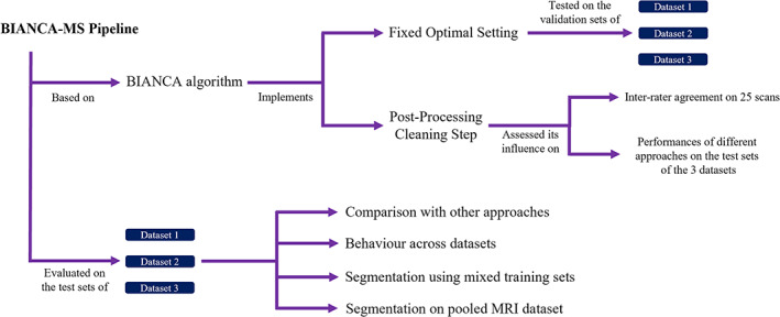
Schematic representation of the BIANCA‐MS pipeline and of the steps performed to validate this new approach.

2.4.3. BIANCA optimization

BIANCA is a flexible, multimodal supervised method based on the k‐nearest neighbor algorithm. Briefly, the algorithm learns the definition of a lesion from a set of manually segmented masks, by using the voxel intensities and the spatial distribution of the intensities as features. BIANCA can be optimized using different options like:

• The possibility of weighting the spatial coordinates (i.e., spatial weighting option) which can increase the accuracy of segmentation, as in some brain regions lesions are more likely to occur.

• The inclusion of intensity information about a small neighborhood of each voxel (patch size option) that can make the segmentation more robust to misregistration and provides local context.

• The selection of the number and the position of training points, which is important to establish to what extent information around lesion edges is crucial for segmentation (i.e., number of training points and Location of non‐lesion training points options). It is possible to separately choose the number of non‐lesion and lesion training points (i.e., voxels per subject). The latter is limited by the number of lesion voxels present in the manual mask.

There are also post‐processing steps to perform on BIANCA outputs: threshold selection and masking. The former highly influences the results: more restrictive thresholds reduce false positives but increase false negatives (Anbeek et al., 2004). The latter consists of applying an exclusion mask for GM and the cerebellum to the BIANCA outputs (Griffanti et al., 2016) to reduce false positives.

To select the optimized BIANCA setting, the training and validation sets of each dataset were used. There were 108 different sets of options used for training BIANCA (Table 4). The parameters that were varied were the spatial weighting (SW), number of lesion and non‐lesion training points (NTP), patch size (PS), and the location of non‐lesion training points (LTP). All the available MRI sequences for each dataset were used, exclusion masks were applied and a threshold of 0.9 was used to obtain the binarized lesion mask. Finally, each of the 108 trained BIANCA models was applied to the validation set of the three datasets (Table 4).

TABLE 4.

The list of the different values tested in this study during the phase of algorithm optimization.

Features	Values tested	Number of options
Spatial weighting (SW)	1–5–10	3
Patch size (PS)	None‐3–6–9	4
Location of non‐WMH training points (LTP)	Surround‐Any‐No Border	3
No. of training points (WMH vs. non‐WMH) (NTP) a	500–1000; 2000–2000; 2000–10000	3
Total combinations		108

^a Number of training points for each training subject. The number of WMH points is capped by the number of voxels available in the manual masks.

2.4.4. Post‐processing cleaning step

Supervised algorithms trained on lesion masks outlined by different users provide slightly different results when applied to new images (Bordin et al., 2021). Further, on a set of images where manual masks are provided by several raters, automated tools can achieve different performance due to the nonidentical way lesions are segmented by the raters. Given this context, inter‐rater variability in lesion contouring could influence algorithm training and evaluation (Shwartzman et al., 2019).

In this work, we proposed a post‐processing cleaning step to reduced unwanted variability in masks that can be applied to both:

• Automatically outlined masks, to further refine lesion segmentation;

• Manually segmented masks, to reduce the impact of the inter‐rater variability on algorithm performance.

This procedure starts by obtaining pure WM, GM, and CSF masks by removing the identified lesion clusters from the three different tissue classes provided by FAST (Y. Zhang et al., 2001). Two stages then follow: a “Recovery” phase to avoid the loss of lesion voxels erroneously not included in lesion mask and a “Refining” phase that aims to create a cleaned lesion mask by considering local intensity contrast and B0 and radiofrequency (RF) inhomogeneity that result in smooth spatial intensity changes throughout the whole image (Figure 2).

FIGURE 2.

Illustration of the cleaning step pipeline using three example lesions, to avoid clutter (example lesions shown with red boxes in the top image). The original lesion mask underwent an initial “Recovery” phase, followed by a two step “Refinement” process. For each phase, the corresponding surrounding WM is depicted. MD, Mahalanobis distance; WM, white matter.

To perform the “Recovery” step, the lesion mask (mask0) were 3D dilated by a single voxel four times ($\mathrm{mas}{\mathrm{k}}_{d1}=\text{dilate}(\text{dilate}\left(\text{dilate}\left(\text{dilate}\left(\text{mask}0\right)\right)\right)$) and only those voxels not adjacent to lesions were retained to form the dilated strip mask ($\text{dilate}{\mathrm{d}}_{\text{strip}}=\mathrm{mas}{\mathrm{k}}_{\mathrm{d}1}-\text{dilate}\left(\text{mask}0\right)$). The WM surrounding the lesions was defined by applying a one voxel 3D dilation ($\mathrm{mas}{\mathrm{k}}_{d2}=\text{dilate}\left(\text{mask}0\right)$), then taking this new dilated strip and masking this by the pure WM masks obtained from FAST:

$$\mathrm{mas}{\mathrm{k}}_{\mathrm{swm}}=\left(\mathrm{mas}{\mathrm{k}}_{d2}-\text{mask}0\right)*\mathrm{mas}{\mathrm{k}}_{\text{purewm}}$$

From this a Mahalanobis distance (MD) was defined at each voxel as:

$$\mathrm{MD}\left(y\right)=\frac{\left|y-{\mu }_{\text{dilated}\_\text{strip}}\right|}{{\sigma }_{\text{dilated}\_\text{strip}}}$$

where y is the intensity of a voxel in mask_swm, while μ _{dilated_strip} and σ _{dilated_strip} are the mean and standard deviation, respectively, of the intensities of all the voxels in the dilated strip. Only those voxels of the surrounding WM with a MD value bigger than a mild threshold (2.0) from the dilated strip were included to form the “recovery lesion” mask ($\mathrm{mas}{\mathrm{k}}_{\mathrm{rec}}$); see “Recovery” in Figure 2.

The “Refining” phase consists of two consecutive steps. In the first refinement step, the intensities of all the voxels from the “recovery lesion” mask were compared to the intensity of the strip of the newly defined surrounding WM (after 3D dilating five times the “recovery lesion” mask)

$$\mathrm{mas}{\mathrm{k}}_{\mathrm{swm}2}=\left(\text{dilated}\left(\text{dilate}\left(\text{dilate}\left(\text{dilate}\left(\text{dilate}\left(\mathrm{mas}{\mathrm{k}}_{\mathrm{rec}}\right)\right)\right)\right)\right)-\mathrm{mas}{\mathrm{k}}_{\mathrm{rec}}\right)*{\text{mask}}_{\text{purewm}})$$

and retained when the MD value was bigger than a sequence‐dependent threshold (4.0 for PD, 7.0 for FLAIR images). This step creates a new “roughly refined” mask ($\mathrm{mas}{\mathrm{k}}_{\mathrm{ref}1}$); see Refine‐step 1 in Figure 2. From $\mathrm{mas}{\mathrm{k}}_{\mathrm{ref}1}$ we removed all the lesions clusters with less than four voxels because lesions below that size are not well defined (Filippi et al., 2019) and thus could impair segmentation reproducibility. Further, these clusters are very likely to be false positive findings of the algorithm. In the second refinement phase, a strip of WM was created by 2D dilating, three times, the “roughly refined” mask.

$$\mathrm{mas}{\mathrm{k}}_{\mathrm{swm}3}=\left(\text{dilate}\left(\text{dilate}\left(\text{dilate}\left({\text{mask}}_{\mathrm{ref}1}\right)\right)\right)-\mathrm{mas}{\mathrm{k}}_{\mathrm{ref}1}\right)*\mathrm{mas}{\mathrm{k}}_{\text{purewm}}$$

All the voxels with a MD distance from the surrounding WM bigger than 4.0 were retained to create the final output. This last step (MD distance calculation and thresholding) was performed separately at each slice of each lesion since differences of intensity due to the RF inhomogeneities lead to systematic differences in the selection criteria of the retained voxels (Refine‐step 2 in Figure 2). The development and optimization of the cleaning step was performed using an internal dataset that was not used in any other analysis. The selection of all the thresholds was done by testing several values for each sequence (e.g., FLAIR or PD images) and choosing the ones that provided the best results upon visual inspection.

To test the impact of this post‐processing cleaning step on inter‐rater agreement, 25 MRI images were selected from the training sets of each Dataset: 5 high resolution FLAIR images from Dataset 1, 10 low resolution FLAIR images from Dataset 2 and 10 low resolution PD images from Dataset 3. These 25 scans were segmented by both experienced raters. Afterwards, the lesion masks obtained were processed with the cleaning procedure and the differences across raters before and after cleaning was assessed (see statistical analysis section for details).

After having assessed its potential capacity to increase the inter‐rater agreement, we established to what extent the cleaning step of the manual masks could influence the performance of the automated tools; since the cleaning procedure was designed to reduce unwanted variability, this additional test could provide, to some extent, a measure of the impact of inter‐rater bias on algorithm performance. To this end, BIANCA was separately trained on the training set of each dataset using the original (i.e., not cleaned) manually segmented lesions masks. Afterwards, we ran the trained algorithms on the corresponding test set. We then evaluated BIANCA performance (without applying any cleaning step to the output) in comparison to the manually segmented masks, both cleaned and not cleaned. The same analysis design, applying the cleaning step to the manual masks of the test sets, was also employed with other tools that are widely used for MS lesion segmentation.

Once the use of the cleaning step on the manual masks was validated, we implemented this post‐processing cleaning step into the BIANCA pipeline, thus obtaining, together with the “optimized setting”, the BIANCA‐MS pipeline. Although the cleaning step was developed as an integral part of BIANCA‐MS pipeline, we performed an additional exploratory analysis to investigate whether our cleaning procedure could increase automated segmentation performance for other tools. To this end, the details of the impact of the cleaning step on the outputs of different automated tools are provided in Data S1.

2.5. BIANCA‐MS evaluation

To evaluate BIANCA‐MS, all the analyses were performed using the test set of each dataset. During algorithm evaluation, the inter‐rater bias was handled into two different ways. First, BIANCA‐MS was trained with the original manual lesion masks (no cleaning applied) as the variability across raters might provide a training procedure that is more heterogeneous and hence richer. Second, on the test set of each dataset, the cleaning procedure was applied to the manual lesions masks to reduce the impact of inter‐rater bias on the performance of the algorithm.

2.5.1. Comparison of BIANCA‐MS with existing algorithms

First, we investigated whether the performance of BIANCA‐MS was similar to those obtained with other existing algorithms. Different automated lesion segmentation algorithms, widely employed as benchmark methods in recent publications on MS lesion segmentation (Cerri et al., 2021; McKinley et al., 2021; Tran et al., 2022; Zhang et al., 2021), were investigated:

• Lesion growth algorithm (LGA, Schmidt et al., 2012) from SPM12 (https://www.applied-statistics.de/lst.html): the algorithm first segments the T1‐W images into the three main tissue classes (CSF, GM, and WM). This information is then combined with the co‐registered FLAIR intensities in order to calculate lesion belief maps. These lesion belief maps are then thresholded with a prechosen initial threshold (κ) to obtain an initial binary lesion map. This mask is subsequently grown along voxels that appear hyperintense in the FLAIR image. This step creates the final lesion probability map output. In this work, the k‐value was set to 0.3 as previously suggested in the original LGA work (Schmidt et al., 2012) and further recommended by Egger et al. (2016) as the value providing the highest and more stable SI.

• Lesion prediction algorithm (LPA, Schmidt, 2017) from SPM12 (https://www.applied-statistics.de/lst.html): LPA requires a FLAIR image only (although also T1‐W images can be provided to the algorithm) and does not require the initial thresholding k‐value. This algorithm consists of a binary classifier in the form of a logistic regression model trained on the data of 53 MS patients with severe lesion patterns. As covariates for this model a similar lesion belief map as for the lesion growth algorithm (Schmidt et al., 2012) was used as well as a spatial covariate that considers voxel‐specific changes in lesion probability. Parameters of this model fit are used to segment lesions in new images by providing an estimate for the lesion probability for each voxel. No preprocessing is applied, because the algorithm performs the necessary bias field correction and affine registration of T1‐W to FLAIR images as part of the pipeline.

• nicMS (Valverde et al., 2017, 2019): the algorithm is a deep learning method based on cascaded convolutional neural networks that, in contrast to most supervised machine learning or deep learning methods, can be used when limited amounts of manual input data are available. In the nicMS approach, WM lesion voxels are inferred using 3D neighboring patch features from a number of different input modalities. To train the nicMS tool, the same training set (number of subjects = 50/40 for Dataset 1 and 2, respectively) and the same modalities used for training BIANCA‐MS were employed. No preprocessing was required, as nicMS internally performs registration, skull‐stripping, and denoising.

• nnUNet (Isensee et al., 2021): the algorithm is a deep learning‐based framework that automatically configures itself for any new segmentation task in the biomedical domain. For each task, the nnUNet runs a five‐fold cross‐validation for three different configurations and automatically performs empirical selection of the optimal ensemble of these models. To train the nnUNet tool, the same training set (number of subjects = 50/40 for Dataset 1 and 2, respectively) used for training BIANCA‐MS were employed. Already co‐registered images were provided to the tool.

• Lesion‐topology preserved anatomical segmentation (Lesion‐TOADS; Le et al., 2019): Lesion‐TOADS requires T1‐W and FLAIR images and is available as a plug‐in for the MIPAV software (http://mipav.cit.nih.gov/). The algorithm embeds an iterative algorithm for fuzzy classification of the image intensities, through a combination of topological and statistical atlases. An additional lesion class is added to the brain segmentation, using the same spatial prior as WM; lesions and WM are then separated by selecting the class with the higher membership value. Already co‐registered and skull‐stripped images were provided to the tool.

As the outputs of LGA, LPA, and nicMS tools are probabilistic, we investigated the impact of a set of different probability thresholds (from 0 to 1 with step size of 0.1) to define a voxel as lesion or not. We then choose the value that gave the highest degree of similarity with the manual masks in the test sets. This step was not performed for nnUNet and Lesion‐TOADS, as these tools output binary lesion masks. Analyses were performed only on Datasets 1 and 2, as the majority of these tools (i.e., LGA, LPA, nicMS, and Lesion‐TOADS) were developed to work using FLAIR sequences. Together with these tools, we also included the original BIANCA algorithm in this comparison analysis. For this, the same probability threshold (0.9) and “optimized” setting implemented in BIANCA‐MS were used when running BIANCA.

2.5.2. BIANCA‐MS behavior across datasets

Second, we tested how BIANCA‐MS behaves for each dataset individually. Thus, BIANCA‐MS was separately trained on each dataset, and for each training case it was run only on the corresponding test set. This provided one set of performance measures for each dataset, which we then used to test the relative performance achieved across the different datasets.

2.5.3. BIANCA‐MS segmentation using mixed training sets

Third, using images acquired in different centers, but with similar acquisition protocols, (Dataset 3) we investigated the influence of using mixed training and test sets on BIANCA‐MS performance. The selection of subjects in training and test sets for Dataset 3 was made in two distinct ways:

• Non‐stratified: sampling is mixed across all centers (as used for the previous analyses)

• Stratified by center: the subjects selected for the training subset belonged to different centers from those used for the test set. This selection criteria (i.e., leave‐one‐center out approach) allowed us to test the cross‐center generalization of BIANCA‐MS.

The number of subjects included in Dataset 3 is the same for each of the two selection methods, but creating distinctly different datasets. We separately trained BIANCA‐MS on the training set of both the stratified and non‐stratified dataset. For each training case, we ran BIANCA‐MS on the corresponding test set and compared the performances achieved on the stratified and non‐stratified datasets.

2.5.4. Evaluation on the pooled MRI dataset

Fourth, we created a global dataset by merging the three datasets. All the images from the three training sets were used for training BIANCA‐MS, whereas the MRI scans from all the different test sets were used for evaluating the algorithm performance. To ensure we used a consistent training and testing procedure, it was necessary to provide to BIANCA‐MS a fixed set of modalities. Thus, we decided to include in the analyses FLAIR and T1‐W images as they are present in both Dataset 1 and 2. For Dataset 3, we created an artificial “PseudoFLAIR” images (Figure 3) by using the following formula (Battaglini et al., 2012):

$$\text{PseudoFlair}:\frac{2\left(\mathrm{PD}*\mathrm{T}2\right)}{\mathrm{PD}+\mathrm{T}2}*\mathrm{T}1$$

FIGURE 3.

Example of a PseudoFLAIR image obtained from PD, T2, and T1‐W on one subject for Dataset 3.

This artificial map, by using intensity information from other sequences, mimics the contrast of FLAIR images (Figure 3). Thus, it is very useful when such sequences are missing (as for Dataset 3). After training the algorithm, we then evaluated the performance of BIANCA‐MS on the combined test set. For the pseudoFLAIR images of Dataset 3, the same lesions masks outlined on the PD images were used.

2.5.5. Validation on the 2016 MSSEG challenge dataset

Finally, we have validated BIANCA‐MS on the MSSEG MICCAI 2016 Challenge dataset (Commowick et al., 2018). This dataset consists of 53 MS subjects whose MRI scans were acquired from three different centers using different scanner manufacturers and magnetic field strengths. These 53 subjects were divided into a training set (n = 15) and a test set (n = 38). Additional details of the dataset are described in Commowick et al., 2018. Together with BIANCA‐MS, we have evaluated all the previously tested tools (i.e., BIANCA, Lesion‐TOADS, LGA, LPA, nicMS, and nnUNet). BIANCA, BIANCA‐MS, nicMS, and nnUNet were trained on the training set of the MICCAI dataset. Then, the trained algorithms, Lesion‐TOADS, LGA, and LPA were run on the test set.

Further, we previously provided a BIANCA‐MS version that was pretrained on a global dataset (obtained by merging three different datasets, see “Evaluation on the pooled MRI dataset” paragraph). Here, we tested its performance on the unseen data of the MICCAI dataset. This analysis could provide crucial information on the possibility of performing lesion segmentation on new MRI data without needing to re‐train the BIANCA‐MS algorithm.

Preprocessed (i.e., denoising, rigid registration, brain extraction, and bias field correction) T1‐W and FLAIR images were used for this experiment. All the images have been delineated by seven experts. Finally, the experts' consensus was used for assessing the tools' performance.

2.6. Performance evaluation

To test the sensitivity, specificity and accuracy of the algorithm, three different metrics (two lesion‐wise metrics and one voxel‐wise) were evaluated: number of false positive clusters (nFPC), defined as the number of clusters (i.e., three‐dimensionally connected voxels) incorrectly labeled as a WM lesion by the algorithm (i.e., no overlap with any voxels labeled as a lesion in the manual masks); number of false negative clusters (nFNC), defined as the number of manually outlined lesions (clusters) that have not been detected by the algorithm (i.e., no overlap with any voxels in the lesion masks output by the algorithm). Voxel‐wise DICE spatial similarity index (SI) defined as

$$\mathrm{SI}=\frac{2*\mathrm{TP}}{2*\mathrm{TP}+\mathrm{FP}+\mathrm{FN}}$$

where TP, FP, and FN are the number of true positive, false positive, and false negative WM lesion voxels, respectively. The SI was calculated for each subject using the whole lesion mask. For each scan, all these metrics were assessed in comparison to either the cleaned or original manual segmentation, depending on the analysis.

2.7. Statistical analyses

All the analyses were performed using MATLAB. Statistical significance was considered when p values were < 0.05. Within each experiment where multiple comparisons were performed, analyses were adjusted using Bonferroni correction.

2.7.1. BIANCA optimization

Optimization step: For each dataset, the 108 different settings were ranked according to median values of the SI, nFPC and nFNC obtained across all the scans of the validation set. As in the original work of BIANCA (Griffanti et al., 2016), the SI index was considered the main metric for determining the rankings. In cases where the SI index was equal, a higher priority for the ranking was then given to nFNC compared to nFPC, as we are interested in achieving high sensitivity for lesion detection. Finally, the setting that had the highest ranking across all the datasets was retained and considered as the common optimal setting. During this optimization phase, performance was assessed using the original (i.e., not cleaned) versions of the manual and automatically obtained lesions masks.

Post‐processing cleaning step: On the 25 high and low‐resolution FLAIR and PD images that had been segmented by both of the two raters, two kinds of analyses were performed.

• Qualitative analysis: to ensure that the proposed cleaning step did not adversely influence the quality of the lesion segmentations, a third rater (RC, a neurologist who is an expert in MRI analysis) blindly assessed the manually delineated lesion masks by each rater, separately, comparing the masks before and after the cleaning procedure is applied. A total of 50 pairs of images were assessed, with each pair consisting of one manual mask without cleaning versus one manual mask with cleaning. These pairs were generated using 25 subjects, with one pair for rater 1 and another, separate, pair for rater 2. A third, independent, rater assigned a “winner” for each pair (i.e., the mask with or without cleaning depending on which was best at outlining the real lesions according to the expert opinion of this third rater). The winning procedure (with or without cleaning) was then defined as the one with more “winners”, as identified by the third rater.

• Quantitative analysis: to measure inter‐rater agreement, the SI indices measured between the lesion segmentations from each rater, on the same subject, both with or both without the cleaning step, were compared using a Wilcoxon signed‐rank test (i.e., each pair uses masks from rater 1 and rater 2).

We further evaluate the influence of the cleaning procedure of the manual masks on the performance of the different tools. To do this, the results achieved by BIANCA, LGA, LPA, nicMS, Lesion‐TOADS, and nnUNet (without cleaning the output) on the test sets were compared between the cases where the manual masks were either all cleaned or not cleaned, using a Wilcoxon signed‐rank test.

2.7.2. BIANCA‐MS evaluation

Comparison of BIANCA‐MS with existing algorithms: SI, nFPC, and nFNC values obtained by BIANCA‐MS and the existing algorithms that we tested were separately compared using the Kruskal–Wallis test. Analyses were adjusted for multiple comparisons using Bonferroni correction. Additionally, the volumetric correlation between each tool's output and the manually segmented mask was assessed using Spearman correlation coefficient.

BIANCA‐MS behavior across datasets: SI, nFPC, and nFNC values obtained by BIANCA‐MS on the three datasets were compared using the Kruskal–Wallis test. Analyses were adjusted for multiple comparison using Bonferroni correction.

BIANCA‐MS segmentation using mixed training sets: The SI, nFPC, and nFNC values obtained by BIANCA‐MS on the third dataset, with and without data stratification per center for the training and test sets, were compared using the Wilcoxon test.

Evaluation on the pooled MRI dataset: SI, nFPC, and nFNC values obtained on the pooled dataset were compared to the ones achieved by BIANCA‐MS on each separate dataset using the Wilcoxon test.

Validation on the 2016 MSSEG challenge dataset: SI, nFPC, and nFNC values obtained by the different tools that we tested were separately compared using the Kruskal–Wallis test. Analyses were adjusted for multiple comparisons using Bonferroni correction.

3. RESULTS

3.1. BIANCA optimization

Table 4 shows the values for each BIANCA parameter that we decided to vary in order to optimize the algorithm. The best five ranked option combinations are listed in Table 5. The first of these top five settings to be common across the three datasets is: an SW value of 5; different number of training points for WMH (2000) and non WMH (10000) classes; local average intensity within a kernel of size of three voxels; and the absence of any location preferences in non‐lesion training points. This setting was chosen as the “optimal setting”, as it had demonstrated that it was the least dependent on the acquisition protocols and therefore should be able to produce outputs with less variation in quality across datasets and hence be used for all datasets without further adaptation required.

TABLE 5.

Rankings of the best five BIANCA settings found based on performance (median ± IQR) in the validation set of each dataset.

	Dataset 1					Dataset 2					Dataset 3
Setting ranking	1	2	3	4	5	1	2	3	4	5	1	2	3	4	5
SW	5	1	1	10	1	1	1	1	5	1	5	5	10	10	5
PS	3	6	9	3	3	9	6	None	3	None	3	None	3	3	6
LTP	Any	Any	Any	Any	Surround	Any	Any	Any	Any	Surround	Any	No Border	No Border	Any	Any
NTP	2000–10000	2000–10000	2000–10000	2000–10000	2000–10000	2000–10000	2000–10000	2000–10000	2000–10000	2000–10000	2000–10000	2000–10000	2000–10000	2000–10000	2000–10000
SI	0.48 ± 0.24	0.48 ± 0.21	0.47 ± 0.22	0.47 ± 0.24	0.46 ± 0.22	0.44 ± 0.23	0.42 ± 0.22	0.42 ± 0.23	0.41 ± 0.22	0.41 ± 0.026	0.51 ± 0.21	0.5 ± 0.2	0.5 ± 0.2	0.5 ± 0.21	0.5 ± 0.2
nFPC	23 ± 20	23 ± 38	25 ± 34	19 ± 13	15 ± 17	53 ± 32	48 ± 22	69 ± 42	26 ± 13	28 ± 19	31 ± 25	49 ± 30	26 ± 20	27 ± 15	25 ± 10
nFNC	2 ± 4	3 ± 5	2 ± 4	3 ± 5	5 ± 6	2 ± 4	2 ± 5	2 ± 4	3 ± 8	5 ± 9	6 ± 5	5 ± 5	7 ± 6	7 ± 6	8 ± 9

Note: The common optimal setting is highlighted in bold.

Abbreviations: LTP, location of WMH training points; nFNC, number of false negative clusters; nFPC, number of false positive clusters; NTP, number of WMH/non‐WMH training points; PS, patch size; SI, dice similarity index; SW, spatial weighting.

3.2. Post‐processing cleaning step

Qualitative analysis: According to the third rater, no relevant differences were detected between the manually segmented and the cleaned lesion masks (25 were better with cleaning, and the other 25 better without cleaning, with no link between better/worse results and a specific rater). This suggests that the two segmentation outputs are indistinguishable.

Quantitative analysis: The implementation of the post‐processing cleaning step strongly increased the spatial overlap between the two raters (SI without cleaning [median ± IQR]: 0.75 ± 0.06; SI with cleaning: 0.87 ± 0.04; p < 0.01; Figure 4).

FIGURE 4.

Example of manual segmentation masks obtained by two raters in both the original version (red and green, second column) and the version where the post‐processing cleaning step is applied (light blue and magenta, third column). Voxel changes between the original and the cleaned lesion mask are shown in the fourth column (orange = voxel in common across the original and cleaned mask, yellow = voxels added by the cleaning step, blue = voxels removed by the cleaning step). White arrows indicate the regions where the raters showed larger differences in lesion contouring. These differences are reduced (light green arrows) when the cleaning step is introduced.

Slight differences in performance were seen when comparing BIANCA output (without cleaning applied to it) to the cleaned and original versions of the manually segmented masks (Table 6). For all the three datasets, a marginal increase of SI was observed when the post‐processing cleaning step was applied to manual masks (p < 0.01). Similarly, cleaning the manually segmented masks increased BIANCA sensitivity (i.e., reducing the nFNC, p < 0.01), albeit to a small extent. Finally, although significance was reached, the application of the cleaning step did not alter nFPC for BIANCA (p < 0.01). As was the case for BIANCA, the application of the cleaning procedure to the manual masks had only a marginal influence on the performance of the other algorithms (note that only the datasets where FLAIR images were provided have been analyzed as the majority of these tools [i.e., LGA, LPA, nicMS, and Lesion‐TOADS] were developed to work using such sequences). Indeed, although in some cases statistical significance was reached, the performance levels achieved were very similar for results obtained using either the cleaned or the original manually segmented masks (Table 6).

TABLE 6.

Tools performance (median ± IQR) assessed in comparison to cleaned and original manual lesions masks.

	Tool	Manual masks	SI	nFPC	nFNC
Dataset 1	BIANCA	Original	0.6 ± 0.24	24 ± 16	4 ± 9
		Clean	0.63 ± 0.25*	24 ± 17*	3 ± 6*
	nicMS	Original	0.67 ± 0.19	8 ± 7	5 ± 7
		Clean	0.67 ± 0.2*	9 ± 7*	4 ± 6*
	LGA	Original	0.33 ± 0.3	1 ± 3	16 ± 18
		Clean	0.33 ± 0.33	1 ± 3	16 ± 17*
	LPA	Original	0.56 ± 0.27	7 ± 8	9 ± 10
		Clean	0.52 ± 0.28	7 ± 8	8 ± 9*
	Lesion‐TOADS	Original	0.47 ± 0.41	69 ± 101	4 ± 7
		Clean	0.51 ± 0.40*	69 ± 102	3 ± 6*
	nnUNet	Original	0.65 ± 0.17	7 ± 7	4 ± 6
		Clean	0.66 ± 0.16*	7 ± 8*	4 ± 6*
Dataset 2	BIANCA	Original	0.63 ± 0.32	18 ± 13	4 ± 11
		Clean	0.66 ± 0.32*	18 ± 14*	3 ± 8*
	nicMS	Original	0.71 ± 0.28	5 ± 9	6 ± 5
		Clean	0.71 ± 0.29*	6 ± 10*	5 ± 6*
	LGA	Original	0.59 ± 0.4	6 ± 6	14 ± 24
		Clean	0.6 ± 0.37*	6 ± 6	13 ± 21*
	LPA	Original	0.59 ± 0.3	18 ± 18	8 ± 11
		Clean	0.6 ± 0.31*	18 ± 18	6 ± 10*
	Lesion‐TOADS	Original	0.23 ± 0.57	43 ± 45	10 ± 16
		Clean	0.25 ± 0.59*	43 ± 45	9 ± 11*
	nnUNet	Original	0.74 ± 0.15	7 ± 8	3 ± 5
		Clean	0.75 ± 0.15	8 ± 10*	3 ± 4*
Dataset 3	BIANCA	Original	0.59 ± 0.25	31 ± 19	10 ± 15
		Clean	0.61 ± 0.27*	31 ± 21	9 ± 10*

Note: For the nicMS, LGA, LPA, Lesion‐TOADS, and nnUNet only the datasets where FLAIR images were provided have been analyzed, as the majority of these tools were developed to work using such sequences.

Abbreviations: nFNC, number of false negative clusters; nFPC, number of false positive clusters; SI, Dice similarity Index.

^*Indicates results where the implementation of the cleaning procedure significantly altered tool performance (p < 0.05).

3.3. Comparison of BIANCA‐MS with existing algorithms

To allow a fair comparison with the SPM, Lesion‐TOADS, and nicMS tools, only the datasets where FLAIR images were provided have been analyzed. For this reason, Dataset 3 was not included in this experiment.

3.3.1. Dataset 1

The optimal lesion probability threshold was 0.4 for nicMS, 0.5 for LPA, and 0 (no threshold) for LGA. Figures 5 and 6 show examples where all the evaluated tools provided generally high and low lesion segmentation performance, respectively, for a single subject. On the test set, the tools showed significantly different SI values (median ± IQR, BIANCA‐MS: 0.72 ± 0.27; BIANCA: 0.63 ± 0.25; Lesion‐TOADS: 0.51 ± 0.40; LGA: 0.33 ± 0.33; LPA: 0.52 ± 0.28; nicMS: 0.67 ± 0.2; nnUNet: 0.66 ± 0.16; p < 0.01). A post‐hoc test revealed how BIANCA‐MS showed the highest SI (p < 0.01). Similarly, overall differences across tools were achieved for nFNC (median ± IQR, BIANCA‐MS: 3 ± 6; Lesion‐TOADS: 3 ± 6; BIANCA: 3 ± 6; LGA: 16 ± 17; LPA: 8 ± 9; nicMS: 4 ± 6; nnUNet: 4 ± 6; p < 0.01). A post‐hoc test revealed how BIANCA‐MS, BIANCA, Lesion‐TOADS, nicMS, and nnUNet showed the lowest nFNC (p < 0.01). Significantly different nFPC were achieved across the different tools: (median ± IQR, BIANCA‐MS: 12 ± 10; BIANCA: 24 ± 17; Lesion‐TOADS: 69 ± 102; LGA: 1 ± 3; LPA: 7 ± 8; nicMS: 9 ± 7; nnUNet: 7 ± 8; p < 0.01). A post‐hoc test revealed how LGA showed the lowest nFPC (p < 0.01). Finally, nicMS showed the highest volumetric correlation (i.e., Spearman correlation coefficients) with the manually outlined masks, followed by nnUNet and BIANCA‐MS (BIANCA‐MS: 0.92; BIANCA: 0.87; nnUNet: 0.94; nicMS: 0.95; LPA = 0.88; LGA = 0.81; Lesion‐TOADS:0.47).

FIGURE 5.

An example of generally high performing lesion segmentations using the different lesion segmentation tools on the same subject from the test set of dataset 1: manual with cleaning applied (turquoise); BIANCA (orange, SI: 0.86, nFPC: 14, nFNC: 3), Lesion‐TOADS (pink, SI: 0.78, nFPC: 20, nFNC: 5), BIANCA‐MS (dark blue, SI: 0.9, nFPC: 8, nFNC: 3), LST‐LGA (red, SI: 0.59, nFPC: 2, nFNC: 16), LST‐LPA (magenta, SI: 0.81, nFPC: 9, nFNC: 9), nicMS (green, SI: 0.82, nFPC: 12, nFNC: 4), and nnUNet (light blue, SI: 0.78, nFPC: 8, nFNC: 4). SI, dice similarity index; nFPC, number of false positive clusters; nFNC, number of false negative clusters.

FIGURE 6.

An example of generally low performing lesion segmentations using the different lesion segmentation tools on the same subject from the test set of dataset 1: manual with cleaning applied (turquoise); BIANCA (orange, SI: 0.51, nFPC: 27, nFNC: 0), Lesion‐TOADS (pink, SI: 0.34, nFPC: 98, nFNC: 1), BIANCA‐MS (dark blue, SI: 0.59, nFPC: 14, nFNC: 7), LST‐LGA (red, SI: 0.02, nFPC: 0, nFNC: 16), LST‐LPA (magenta, SI: 0.3, nFPC: 6, nFNC: 9), nicMS (green, SI: 0.53, nFPC: 15, nFNC: 1), and nnUNet (light blue, SI: 0.66, nFPC: 7, nFNC: 1). SI, dice similarity index; nFPC, number of false positive clusters; nFNC, number of false negative clusters.

3.3.2. Dataset 2

The optimal lesion probability threshold was 0.3 for nicMS, 0.4 for LPA, and 0.2 for LGA. Figures 7 and 8 show examples where all the evaluated tools provided generally high and low lesion segmentation performance, respectively, for a single subject. On the test set, the tools showed significantly different SI values (median ± IQR, BIANCA‐MS: 0.75 ± 0.33; BIANCA: 0.66 ± 0.32; Lesion‐TOADS: 0.25 ± 0.59; LGA: 0.6 ± 0.37; LPA: 0.6 ± 0.31; nicMS: 0.71 ± 0.29; nnUNet: 0.75 ± 0.15; p < 0.01). A post‐hoc test revealed how BIANCA‐MS and nnUNet showed the highest SI (p < 0.01). Significant differences were achieved for nFNC (median ± IQR, BIANCA‐MS: 3 ± 8; BIANCA: 3 ± 8; Lesion‐TOADS: 9 ± 11; LGA: 13 ± 21; LPA: 6 ± 10; nicMS: 5 ± 6; nnUNet: 3 ± 4; p < 0.01). A post‐hoc test revealed how BIANCA‐MS, BIANCA, nicMS, and nnUNet showed the lowest nFNC (p < 0.01). Significantly different nFPC results were achieved across the different tools: (median ± IQR, BIANCA‐MS: 15 ± 10; BIANCA: 18 ± 14; Lesion‐TOADS: 43 ± 45; LGA: 6 ± 6; LPA: 18 ± 18; nicMS: 6 ± 10; nnUNet: 8 ± 10; p < 0.01). A post‐hoc test revealed how LGA and nicMS showed the lowest nFPC (p < 0.01). Finally, nicMS and nnUNet showed the highest volumetric correlation with the manually outlined masks, followed by BIANCA‐MS and LGA (BIANCA‐MS: 0.95; BIANCA: 0.89; nnUNet: 0.98; nicMS: 0.98; LPA = 0.93; LGA = 0.94; Lesion‐TOADS: 0.15).

FIGURE 7.

An example of generally high performing lesion segmentations using the different lesion segmentation tools on the same subject from the test set of dataset 2: manual with cleaning applied (turquoise); BIANCA (orange, SI:0.79, nFPC: 12, nFNC: 6), Lesion‐TOADS (pink, SI: 0.7, nFPC: 2, nFNC: 7), BIANCA‐MS (dark blue, SI: 0.94, nFPC: 6, nFNC 23), LST‐LGA (red, SI: 0.7, nFPC:2, nFNC: 32), LST‐LPA (magenta, SI: 0.78, nFPC: 18, nFNC:10), nicMS (green, SI: 0.81, nFPC: 11, nFNC: 6), and nnUNet (light blue, SI: 0.83, nFPC: 11, nFNC: 4). SI, dice similarity index; nFPC, number of false positive clusters; nFNC, number of false negative clusters.

FIGURE 8.

An example of generally low performing lesion segmentations using the different lesion segmentation tools on the same subject from the test set of dataset 2: manual with cleaning applied (turquoise); BIANCA (orange, SI:0.44, nFPC: 12, nFNC: 26), Lesion‐TOADS (pink, SI: 0.24, nFPC: 60, nFNC: 14), BIANCA‐MS (dark blue, SI: 0.62, nFPC: 12, nFNC: 4), LST‐LGA (red, SI: 0.21, nFPC: 7, nFNC: 41), LST‐LPA (magenta, SI: 0.42, nPC: 32, nFNC: 21), nicMS (green, SI: 0.59, nFPC: 7, nFNC: 7), and nnUNet (light blue, SI: 0.7, nFPC: 23, nFNC: 6). SI, dice similarity index; nFPC, number of false positive clusters; nFNC, number of false negative clusters.

3.4. BIANCA‐MS behavior across datasets

When BIANCA‐MS was run on the three test sets, no differences were found for SI (median ± IQR, Dataset 1: 0.72 ± 0.27; Dataset 2: 0.75 ± 0.33; Dataset 3: 0.7 ± 0.29). Significantly different nFNC results were obtained across datasets (median ± IQR, Dataset 1: 3 ± 6; Dataset 2: 3 ± 8; Dataset 3: 8 ± 11; p < 0.01). A post‐hoc test revealed how the highest nFNC was achieved on Dataset 3 (p < 0.01). BIANCA‐MS showed significantly different nFPC results across datasets (median ± IQR, Dataset 1: 12 ± 10; Dataset 2: 15 ± 10; Dataset 3: 16 ± 14; p < 0.01). A post‐hoc test revealed increased nFPC in Dataset 3 compared to Dataset 1 (p < 0.01).

3.5. BIANCA‐MS segmentation using mixed training sets

No statistically significant differences were found for SI, nFPC, and nFNC when BIANCA‐MS was trained on the stratified versus the non‐stratified datasets (Table 7).

TABLE 7.

Comparison of BIANCA‐MS performances (median ± IQR) measures using the stratified and non‐stratified sets extracted from Dataset 3 (to test for cross‐center generalization).

	SI	nFPC	nFNC
Non‐stratified dataset 3	0.7 ± 0.29	16 ± 14	8 ± 11
Stratified dataset 3	0.68 ± 0.3	17 ± 13	12 ± 13

Note: None of the statistical tests were significant here.

Abbreviations: nFNC, number of false negative clusters; nFPC, number of false positive clusters; SI, dice similarity Index.

3.6. Evaluation on pooled MRI datasets

No differences were found in BIANCA‐MS performance when the tool was trained and evaluated using images acquired with different scanning protocols (median ± IQR, SI: 0.72 ± 0.25; nFPC: 13 ± 11; nFNC: 4 ± 8) and when each dataset is separately analyzed (median ± IQR across datasets, SI: 0.72 ± 0.28; nFPC: 14 ± 11; nFNC: 4 ± 8).

3.7. Validation on the 2016 MSSEG challenge dataset

The optimal lesion probability threshold was 0.1 for LGA, 0.2 for LPA, and 0.9 for nicMS. On the test set, the tools showed significantly different SI values (Table 8; p < 0.01). A post‐hoc test revealed how nnUNet, BIANCA‐MS (both the versions trained on the global and MICCAI dataset) and nicMS showed the highest SI (p < 0.01). Similarly, overall differences across tools were achieved for nFNC (Table 8; p < 0.01). A post‐hoc test revealed how nicMS and nnUNet achieved the lowest nFNC (p < 0.01). Significantly different nFPC were achieved across the different tools (Table 8; p < 0.01). A post‐hoc test revealed how nnUNet showed the lowest nFPC (p < 0.01).

TABLE 8.

Tools performance (median ± IQR) on the test set of the MICCAI 2016 dataset.

	SI	nFPC	nFNC
BIANCA	0.64 ± 0.41	78 ± 108	6 ± 19
BIANCA‐MS (MICCAI trained)	0.72 ± 0.3*	26 ± 30	8 ± 18
BIANCA‐MS (global dataset trained)	0.7 ± 0.3*	23 ± 29	11 ± 18
LGA	0.48 ± 0.43	10 ± 20	17 ± 28
LPA	0.57 ± 0.37	51 ± 76	10 ± 24
Lesion‐TOADS	0.46 ± 0.34	12 ± 22	14 ± 33
nicMS	0.7 ± 0.39*	9 ± 12	5 ± 13*
nnUNet	0.76 ± 0.25*	4 ± 4*	6 ± 12*

Abbreviations: nFNC, number of false negative clusters; nFPC, number of false positive clusters; SI, dice similarity index.

^*Indicates results where the tools provided significantly higher performance (p < 0.05).

4. DISCUSSION

In this work we presented BIANCA‐MS, a novel automated procedure for the segmentation of WM brain lesions in MS. This tool has been validated on MR images acquired using different scanners, imaging protocols, and resolutions, demonstrating that it is robust, flexible, and accurate. With the pipeline proposed here, we wanted to overcome some of the main issues limiting AI tool generalization and their implementation in medical imaging: the identification of a unique set of parameters able to deal with a variety of scanning protocols and the variability in results induced by inter‐rater variability.

The first contribution of this study is the unique set of parameter values, identified after a large optimization procedure, which proved to be relatively independent from scanning protocol and should reflect typical MS lesion features (SW = 5, PS = 3, LTP = any, NTP WMH/non‐WMH = 2000/10000). The selection of a value of 5 for the SW option was most likely needed due to the specific regional distribution of MS lesions (Filippi et al., 2019). The absence of any regional preferences in local non‐WMH voxels for the training (LTP option) could be due to the variability of MS lesion borders, which can be either sharp or ill‐defined (Lucchinetti et al., 2000). Since the inflammation process could affect brain regions differently, the inclusion of intensity information about a small neighborhood of each lesion (PS option) proved to improve algorithm accuracy (Lao et al., 2008). The imbalance in the number of training voxels between WMH and non‐WMH was related to the wide heterogeneity of non‐WMH voxels. Thus, a higher number of non‐WMH voxels was needed to better depict non‐lesional tissues. In the original work of BIANCA (Griffanti et al., 2016), it was demonstrated that the tool does not benefit much from increasing these numbers (e.g., 10000 WMH, 58000 non‐WMH) and it could provide accurate segmentation with a modest number of training points (i.e., 2000 WMH, 10000 non WMH). Given this context, we have decided not to test bigger values and instead focus on investigating whether BIANCA‐MS could provide accurate lesion segmentations with fewer training points. Importantly, the set of parameter values proved to be relatively independent of the acquisition protocol, the set of images provided, image resolution and main modality of reference, based on the fact that this same set of values (out of 108 possibilities) ranked within the top five sets for all datasets. Therefore, the use of this harmonized setting could avoid the complex and time‐consuming optimization procedures needed for adapting algorithm parameters to each dataset. In the original work of BIANCA, different optimal settings were found (Griffanti et al., 2016). This is likely to be related to the different spatial location, shape, and contrast between WMHs of presumed vascular origin and MS lesions.

Another crucial and innovative step of the BIANCA‐MS pipeline is the cleaning procedure. The implementation of this approach was motivated by evidence of the impact of inter‐rater bias on segmentation (Shwartzman et al., 2019). This is of great relevance if we consider that automated tools are usually validated in comparison to manual segmentation. These segmentations are highly subjective and difficult to reproduce, thus resulting in an insufficiently reliable gold standard. In this work, the application of the cleaning step significantly increased the concordance across raters, thus reducing this source of variability when validating automated tools. Moreover, the absence of any qualitative difference between the lesion masks with and without the cleaning procedure, as verified by our third, blinded expert rater, suggested that our pipeline reduced the inter‐rater variability without influencing the overall quality of the initial segmentation. As proof of this, the application of the cleaning procedure to the manually segmented masks had only a marginal effect on the performance of the automated tools. Further, although the cleaning procedure was developed to be an integral part of the BIANCA‐MS pipeline, we have tried applying our refinement step to the nicMS, LGA, LPA, Lesion‐TOADS, and nnUNet outputs (see Data S1). The results obtained highlighted a general increase of the tools' performance when the automated outputs were cleaned. These findings suggested that the cleaning procedure could be used on any automatically obtained lesion masks, irrespective of the tool employed. Several strategies have been proposed to refine lesion segmentation, including the use of lesion location information (Datta & Narayana, 2013), continuity across slices (Abdullah et al., 2011), ratio maps across modalities (Sajja et al., 2006) and classification of FP as outlier clusters far from lesion and not lesion tissues (Lao et al., 2008). Other approaches simultaneously employed information coming from different sources (Abdullah et al., 2011; Battaglini et al., 2014; Ganna et al., 2002; Khastavaneh & Haron, 2014; Roura et al., 2015). A point of strength of our pipeline is that it relies on the objective analysis of the intensity distribution of the pure tissues surrounding the lesions in both 3D and 2D, which solves the problem of local inhomogeneities strongly influencing lesion segmentation. A possible drawback is that the cleaning step refines lesion segmentation using the pure WM, GM, and CSF masks obtained by the FAST tool. Artefacts, low‐contrast or noisy images could hamper the FAST segmentation process, thus in turn influencing the overall results of the cleaning step pipeline. Although future studies are needed to further test the reliability of the approach, the large variability in MRI data analyzed here, and the results obtained, demonstrate the robustness of our approach.

BIANCA‐MS clearly outperformed all the existing tools (with the exception of the nnUNet on Dataset 2) that we evaluated in terms of SI in both Dataset 1 and 2. Lesion‐TOADS ranked the lowest in terms of the SI value whereas nnUNet, nicMS, BIANCA, and LPA ranked second, third, fourth, and fifth, respectively. Together with BIANCA, nicMS and nnUNet, BIANCA‐MS achieved, on both datasets, the lowest nFNC, thus proving the high sensitivity of the approach. LGA showed the highest nFNC, providing overall the worst performance across all the tools. BIANCA‐MS showed lower precision in lesion detection (i.e., higher nFPC) in comparison to nicMS, LGA, and nnUNet. However, the larger nFPC results did not substantially alter the SI achieved by our approach. On both high and low‐resolution images, BIANCA‐MS, nicMS, and nnUNet showed consistently high volumetric correlation with the manually outlined masks, whereas LGA and LPA showed relatively lower degrees of concordance, especially on the 2D acquired images. Lesion‐TOADS achieved the lowest volumetric correlation among all the evaluated tools. Taken together, our findings suggest that BIANCA‐MS provided overall the best performance across all the evaluated tools. Similarly, in an additional experiment performed on the MICCAI 2016 challenge dataset, BIANCA‐MS achieved the second‐best performance in terms of SI while showing nFNC values in range with the other tools. As was for the case of Dataset 1 and 2, BIANCA‐MS showed higher nFPC. However, this did not seem to influence the SI achieved. Although future studies are needed to further reduce the nFPC identified by our approach, the results achieved on the MICCAI dataset confirmed the overall accuracy of BIANCA‐MS. It is worth noting that these results could be influenced by the way we selected the optimal thresholds for the tools: we used SI as the main metric, giving more importance to achieving lower nFNC (i.e., higher sensitivity) than lower nFPC (i.e., higher precision). Thus, different selection criteria might provide different results. Importantly, the nicMS, LST tools, and Lesion‐TOADS require FLAIR images as a predefined reference modality; thus, although artificial pseudoFLAIR images were provided, Dataset 3 was excluded to allow a fair comparison across tools. In contrast, BIANCA‐MS is very flexible in terms of modalities and can perform segmentation using any set of images provided. Further, several studies have reported variations in the performance of algorithms across datasets (Griffanti et al., 2016; Guo et al., 2019; Roura et al., 2015), even with consistent scanner field strength and after protocol harmonization (Shinohara et al., 2017). The consistency of the performance measures obtained here across datasets demonstrates the robustness and flexibility of BIANCA‐MS when different acquisition protocols, image modalities and resolutions are provided to the algorithm.

BIANCA‐MS performance was dependent on lesion load and size (see Data S1), which is well established in the literature where it has been repeatedly shown that automated lesion segmentation performance increases with higher lesion load and with lesions with larger volumes (Commowick et al., 2018; Gabr et al., 2020; Jain et al., 2015). Considering this, and the inclusion criteria we adopted for dividing each dataset into three subsets, it is not particularly surprising that higher performances were found in the test sets (subjects with variable lesion load) compared to the validation sets (subjects with low lesion load). BIANCA‐MS achieved a higher performance with periventricular lesions, followed by deep‐WM and juxtacortical lesions (see Data S1). To elucidate this finding, two factors should be considered. First, periventricular lesions showed larger volumes compared to deep‐WM and juxtacortical lesions. Second, we previously demonstrated that BIANCA‐MS performance was dependent on lesion load and size. Taken together, these two factors could explain the differences in BIANCA‐MS performance across different regions.

It is also worth noting that BIANCA‐MS performed slightly better (although not significantly) on FLAIR‐3D images. Algorithms are validated using mostly images with 2D/slice‐wise acquisitions, with only a small number of images with 3D acquisitions employed, often utilizing online databases. In this respect, we did not limit our analyses to images with 2D acquisitions, but we extensively evaluated BIANCA‐MS, to the best of our knowledge, on one of the biggest private datasets of MS subjects where images with 3D acquisitions have been manually segmented. The results achieved are of the utmost relevance if we consider that high resolution FLAIR‐3D sequences are now the preferred acquisition due to their high sensitivity in lesion detection (Bravo et al., 2014; Filippi et al., 2019), and thus in the future such high‐resolution images will be more and more commonly acquired.

Another key observation in our study is that training BIANCA‐MS on stratified or non‐stratified data did not influence the performance of the algorithm. In clinical trials, the accrual of WM lesions is one of the most commonly used MRI outcomes (van Munster & Uitdehaag, 2017) and images are acquired from different centers. Thus, an automatic segmentation tool that provides accurate and robust segmentation of WM lesions in multicenter data is greatly needed. The results of this study highlight how BIANCA‐MS is insensitive to data stratification per center, making it easier to apply in clinical trials where training with data from the same center is difficult or impossible, whereas mixed training sets are straightforward. Further, by using a leave‐one‐center out approach, we have demonstrated the cross‐center generalization abilities of BIANCA‐MS (i.e., testing performance on data from an unseen center) as this analysis was based on MRI data acquired from different centers and different scanners. However, all the data were acquired using a similar MRI protocol. Thus, future studies are needed to further test BIANCA‐MS performance on a wider set of MRI protocols. In a recent work, a similar cross validation approach was performed (Gabr et al., 2020). Our results are in line with those obtained by Gabr et al.; however, we did not focus only on SI, but we also included nFPC and nFNC as further analysis metrics.

Finally, the introduction of PseudoFLAIR images allowed the creation of a global multicenter dataset. When trained on this unified dataset, the performance of BIANCA‐MS was comparable to the ones achieved when separately trained on each center. Lesion segmentation across heterogeneous acquisition protocols is a challenging task, with studies reporting only poor (Heinen et al., 2019) to moderate reproducibility across centers (de Sitter et al., 2017). Recently, an AI tool demonstrated high consistency across a wide range of imaging parameters (Duong et al., 2019). However, the large amount of training data (n = 295) needed to achieve such performance could limit its use in a real‐world setting. Pooling MRI data represents a very practical solution for increasing both the external validity and transposability of research findings to clinical settings (Heinen et al., 2019). Further, training AI tools on more heterogeneous data increases the performance in out of distribution (OOD) MRI data (Mårtensson et al., 2020). In this respect, by using the OOD data of the MICCAI dataset, we obtained results from the BIANCA‐MS version pretrained on the global dataset that were superior or comparable to the other tested tools (including the BIANCA‐MS version trained on the training set of the MICCAI dataset). Given this, we hope large multicenter datasets will be more and more employed in the future. The wide training procedure is likely to further the performance of BIANCA‐MS for lesion segmentation in OOD MRI data, avoiding the need to be retrained.

This study is not without limitations. First, BIANCA‐MS is not completely automatic, as it needs to be retrained whenever applied to data acquired with different acquisition protocols. Some pretrained tools (e.g., nicMS) can be retrained and tuned on a new dataset with a small number of subjects. However, their performance is noticeably inferior with respect to when the same tools are fully trained on a larger dataset (Weeda et al., 2019). The possibility of retraining BIANCA‐MS using a small number of subjects has not been tested in this work. However, in this work, we have demonstrated that training BIANCA‐MS on a global dataset (obtained by merging the three different datasets) did not influence the performance of the tool, even when tested on the OOD data of the MICCAI 2016 dataset. This introduces the possibility of obtaining a BIANCA‐MS version that is pretrained on some large datasets and can perform lesion segmentation on new MRI data without needing to be retrained. Although the BIANCA‐MS version trained on a global dataset we provided in the current work showed promising results, its performance on an even wider variety of unseen data has not been tested yet and will require future studies. Second, we focused on segmenting WM lesions, employing an exclusion mask that covers cerebellum and grey matter (GM). Usually, lesions in the cerebellum and close to the GM are not easily detectable on conventional MR images (García‐Lorenzo et al., 2013). Further, FLAIR images typically present hyperintensities in cortical areas and flow artefacts around the fourth ventricle which can negatively impact the lesion detection. This is certainly a potential area for further improvement of this promising tool. Future efforts could address the implementation of sequences able to improve juxtacortical, cerebellar, and GM lesion detection (Geurts et al., 2005; Nelson et al., 2007). Third, the cleaning step has been shown to create perceptually equivalent lesion masks, as rated by an expert neurologist, while substantially improving inter‐rater agreement, and hence was used to create the gold standard employed here. It also has been used as part of the BIANCA‐MS method, to improve performance. This improvement is likely to be partly due to improved delineation of the lesions, and thus reducing erroneous mismatches, and partly due to the positive bias of using the same cleaning step for both inputs and outputs. To assess this effect, the cleaning step was also applied to the output of the other tools, which showed mixed results from no improvement to substantial improvement (see Data S1). Fourth, the DICE was considered the main index for evaluating the tools' performance. This metric can provide a biased estimation of the segmentation accuracy due to the influence of large lesions (Ma et al., 2022). The number of false positive and negative lesions might be more appropriate from a clinical perspective and these were also included in our results. However, the DICE index is the most common metric reported in the segmentation literature, hence our choice to use it as main metric in the present work. Further, we gave a higher priority to FN compared to FP as we are more interested in achieving high sensitivity, since a manual review of identified lesions to filter out FPs is more efficient than finding FNs, as the latter involves carefully inspecting the entire image. As a consequence, the number of false positives in the BIANCA‐MS output is relatively high, but these are mostly small clusters (mean volume ± SD, 0.0394 ± 0.0894 cm³, 0.0279 ± 0.0599 cm³, and 0.0723 ± 0.17 cm³ for Datasets 1, 2, and 3, respectively). Lesion identification, especially for new lesions, is a key biomarker in MS diagnosis and thus, future studies are needed to assess and improve the specificity of BIANCA‐MS. In this respect, it would be fundamental to assess the number of false positive clusters found in healthy subjects; such analysis will provide crucial information for any implementation of BIANCA‐MS in clinical practice. Finally, future efforts will address the development of a longitudinal BIANCA‐MS pipeline.

To conclude, in this work we have presented BIANCA‐MS, a novel automated procedure developed to overcome some of the issues limiting the generalizability of results achieved by AI tools. On two internal datasets, our method clearly outperformed other available tools and proved to be robust, accurate and flexible across different scanning protocols. Furthermore, the insensitivity of BIANCA‐MS to data stratification per center makes it suitable when a mixed training set is provided, as in clinical trial settings. Thirdly, pooling MRI data acquired with different scanning protocols did not influence the performance of BIANCA‐MS, even when tested on new unseen MRI data. This introduces the possibility of obtaining a BIANCA‐MS version that is pretrained on some large datasets and can perform lesion segmentation on new MRI data without needing to be retrained. Finally, using the open MICCAI dataset, the performance of BIANCA‐MS placed within the top ranks among the evaluated tools. These encouraging results suggested that BIANCA‐MS is a promising tool for the segmentation of WM brain lesions in MS.

AUTHOR CONTRIBUTIONS

Conceptualization: Giordano Gentile, Mark Jenkinson, Ludovica Griffanti, Nicola De Stefano, and Marco Battaglini. Formal analysis: Giordano Gentile. Investigation: Giordano Gentile, Mark Jenkinson, Ludovica Griffanti, Matteo Leoncini, Maira Inderyas, Marzia Mortilla, Nicola De Stefano, Rosa Cortese, and Marco Battaglini. Methodology: Giordano Gentile, Matteo Leoncini, Maira Inderyas, Marzia Mortilla, Rosa Cortese, and Marco Battaglini. Visualization: Giordano Gentile. Writing—original draft: Giordano Gentile and Marco Battaglini. Writing—review and editing: Giordano Gentile, Mark Jenkinson, Ludovica Griffanti, Ludovico Luchetti, Matteo Leoncini, Maira Inderyas, Marzia Mortilla, Rosa Cortese, Nicola De Stefano, and Marco Battaglini. Supervision: Mark Jenkinson, Ludovica Griffanti, Rosa Cortese, Nicola De Stefano, and Marco Battaglini.

CONFLICT OF INTEREST STATEMENT

Mark Jenkinson receives royalties from Oxford University Innovations for licensing of the FSL software for commercial, non‐academic use. The remaining authors report no financial interests or potential conflicts of interest for this work.

Supporting information

 

Data S1. Supporting Information.

Gentile, G. , Jenkinson, M. , Griffanti, L. , Luchetti, L. , Leoncini, M. , Inderyas, M. , Mortilla, M. , Cortese, R. , De Stefano, N. , & Battaglini, M. (2023). BIANCA‐MS: An optimized tool for automated multiple sclerosis lesion segmentation. Human Brain Mapping, 44(14), 4893–4913. 10.1002/hbm.26424

DATA AVAILABILITY STATEMENT

Data and code availability statement: Individual MRI participant data cannot be made openly available due to privacy issues of clinical data. The software we presented in this work (BIANCA‐MS) is based on the algorithm named BIANCA, which is freely available as part of the FSL (FMRIB Software Library) package (https://fsl.fmrib.ox.ac.uk/fsl/fslwiki). The post‐processing analysis step code we developed in this work will be made available for research purpose upon approval of the corresponding author.

REFERENCES

- Abdullah, B. A. , Younis, A. A. , Pattany, P. M. , & Saraf‐Lavi, E. (2011). Textural based SVM for MS lesion segmentation in FLAIR MRIs. Open Journal of Medical Imaging, 1(2), 26–42. 10.4236/OJMI.2011.12005 [DOI] [Google Scholar]
- Anbeek, P. , Vincken, K. L. , van Osch, M. J. P. , Bisschops, R. H. C. , & van der Grond, J. (2004). Probabilistic segmentation of white matter lesions in MR imaging. Neuroimage, 21(3), 1037–1044. 10.1016/j.neuroimage.2003.10.012 [DOI] [PubMed] [Google Scholar]
- Balakrishnan, R. , Hernández, M. C. V. , & Farrall, A. J. (2021). Automatic segmentation of white matter hyperintensities from brain magnetic resonance images in the era of deep learning and big data–a systematic review. Computerized Medical Imaging and Graphics, 88, 101867. 10.1016/J.COMPMEDIMAG.2021.101867 [DOI] [PubMed] [Google Scholar]
- Battaglini, M. , de Stefano, N. , & Jenkinson, M. (2012). A fully automated, hierarchical classification method for detecting white matter lesions in multiple sclerosis. Proceedings of the International Society for Magnetic Resonance in Medicine, 20. [Google Scholar]
- Battaglini, M. , Rossi, F. , Grove, R. A. , Stromillo, M. L. , Whitcher, B. , Matthews, P. M. , & de Stefano, N. (2014). Automated identification of brain new lesions in multiple sclerosis using subtraction images. Journal of Magnetic Resonance Imaging: JMRI, 39(6), 1543–1549. 10.1002/JMRI.24293 [DOI] [PubMed] [Google Scholar]
- Bordin, V. , Bertani, I. , Mattioli, I. , Sundaresan, V. , McCarthy, P. , Suri, S. , Zsoldos, E. , Filippini, N. , Mahmood, A. , Melazzini, L. , Laganà, M. M. , Zamboni, G. , Singh‐Manoux, A. , Kivimäki, M. , Ebmeier, K. P. , Baselli, G. , Jenkinson, M. , Mackay, C. E. , Duff, E. P. , & Griffanti, L. (2021). Integrating large‐scale neuroimaging research datasets: Harmonisation of white matter hyperintensity measurements across Whitehall and UK biobank datasets. Neuroimage, 237, 118189. 10.1016/J.NEUROIMAGE.2021.118189 [DOI] [PMC free article] [PubMed] [Google Scholar]
- Bravo, P. , Sánchez Hernández, J. J. , Ibáñez Sanz, L. , Alba De Cáceres, I. , Crespo San José, J. L. , & García‐Castaño Gandariaga, B. (2014). A comparative MRI study for white matter hyperintensities detection: 2D‐FLAIR, FSE PD 2D, 3D‐FLAIR and FLAIR MIP. The British Journal of Radiology, 87(1035), 20130360. 10.1259/BJR.20130360 [DOI] [PMC free article] [PubMed] [Google Scholar]
- Brownlee, W. J. , Altmann, D. R. , Prados, F. , Miszkiel, K. A. , Eshaghi, A. , Gandini Wheeler‐Kingshott, C. A. M. , Barkhof, F. , & Ciccarelli, O. (2019). Early imaging predictors of long‐term outcomes in relapse‐onset multiple sclerosis. Brain: A Journal of Neurology, 142(8), 2276–2287. 10.1093/BRAIN/AWZ156 [DOI] [PubMed] [Google Scholar]
- Cerri, S. , Puonti, O. , Meier, D. S. , Wuerfel, J. , Mühlau, M. , Siebner, H. R. , & van Leemput, K. (2021). A contrast‐adaptive method for simultaneous whole‐brain and lesion segmentation in multiple sclerosis. Neuroimage, 225, 117471. 10.1016/J.NEUROIMAGE.2020.117471 [DOI] [PMC free article] [PubMed] [Google Scholar]
- Commowick, O. , Istace, A. , Kain, M. , Laurent, B. , Leray, F. , Simon, M. , Pop, S. C. , Girard, P. , Améli, R. , Ferré, J. C. , Kerbrat, A. , Tourdias, T. , Cervenansky, F. , Glatard, T. , Beaumont, J. , Doyle, S. , Forbes, F. , Knight, J. , Khademi, A. , … Barillot, C. (2018). Objective evaluation of multiple sclerosis lesion segmentation using a data management and processing infrastructure. Scientific Reports, 8(1), 1–17. 10.1038/s41598-018-31911-7 [DOI] [PMC free article] [PubMed] [Google Scholar]
- Danelakis, A. , Theoharis, T. , & Verganelakis, D. A. (2018). Survey of automated multiple sclerosis lesion segmentation techniques on magnetic resonance imaging. Computerized Medical Imaging and Graphics, 70, 83–100. 10.1016/J.COMPMEDIMAG.2018.10.002 [DOI] [PubMed] [Google Scholar]
- Datta, S. , & Narayana, P. A. (2013). A comprehensive approach to the segmentation of multichannel three‐dimensional MR brain images in multiple sclerosis. Neuroimage Clinical, 2(1), 184–196. 10.1016/J.NICL.2012.12.007 [DOI] [PMC free article] [PubMed] [Google Scholar]
- de Sitter, A. , Steenwijk, M. D. , Ruet, A. , Versteeg, A. , Liu, Y. , van Schijndel, R. A. , Pouwels, P. J. W. , Kilsdonk, I. D. , Cover, K. S. , van Dijk, B. W. , Ropele, S. , Rocca, M. A. , Yiannakas, M. , Wattjes, M. P. , Damangir, S. , Frisoni, G. B. , Sastre‐Garriga, J. , Rovira, A. , Enzinger, C. , … Vrenken, H. (2017). Performance of five research‐domain automated WM lesion segmentation methods in a multi‐center MS study. Neuroimage, 163, 106–114. 10.1016/J.NEUROIMAGE.2017.09.011 [DOI] [PubMed] [Google Scholar]
- Duong, M. T. , Rudie, J. D. , Wang, J. , Xie, L. , Mohan, S. , Gee, J. C. , & Rauschecker, A. M. (2019). Convolutional neural network for automated FLAIR lesion segmentation on clinical brain MR imaging. AJNR American Journal of Neuroradiology, 40(8), 1282–1290. 10.3174/AJNR.A6138 [DOI] [PMC free article] [PubMed] [Google Scholar]
- Egger, C. , Opfer, R. , Wang, C. , Kepp, T. , Sormani, M. P. , Spies, L. , Barnett, M. , & Schippling, S. (2016). MRI FLAIR lesion segmentation in multiple sclerosis: Does automated segmentation hold up with manual annotation? Neuroimage: Clinica, 13, 264–270. 10.1016/J.NICL.2016.11.020 [DOI] [PMC free article] [PubMed] [Google Scholar]
- Filippi, M. , Preziosa, P. , Banwell, B. L. , Barkhof, F. , Ciccarelli, O. , De Stefano, N. , Geurts, J. J. G. , Paul, F. , Reich, D. S. , Toosy, A. T. , Traboulsee, A. , Wattjes, M. P. , Yousry, T. A. , Gass, A. , Lubetzki, C. , Weinshenker, B. G. , & Rocca, M. A. (2019). Assessment of lesions on magnetic resonance imaging in multiple sclerosis: Practical guidelines. Brain: A Journal of Neurology, 142(7), 1858–1875. 10.1093/BRAIN/AWZ144 [DOI] [PMC free article] [PubMed] [Google Scholar]
- Gabr, R. E. , Coronado, I. , Robinson, M. , Sujit, S. J. , Datta, S. , Sun, X. , Allen, W. J. , Lublin, F. D. , Wolinsky, J. S. , & Narayana, P. A. (2020). Brain and lesion segmentation in multiple sclerosis using fully convolutional neural networks: A large‐scale study. Multiple Sclerosis (Houndmills, Basingstoke, England), 26(10), 1217–1226. 10.1177/1352458519856843 [DOI] [PMC free article] [PubMed] [Google Scholar]
- Ganna, M. , Rombaut, M. , Goutte, R. , & Zhu, Y. M. (2002). Improvement of brain lesions detection using information fusion approach. 6th international conference on signal processing proceedings, Beijing, China. [Google Scholar]
- García‐Lorenzo, D. , Francis, S. , Narayanan, S. , Arnold, D. L. , & Collins, D. L. (2013). Review of automatic segmentation methods of multiple sclerosis white matter lesions on conventional magnetic resonance imaging. Medical Image Analysis, 17(1), 1–18. 10.1016/J.MEDIA.2012.09.004 [DOI] [PubMed] [Google Scholar]
- Geurts, J. J. G. , Pouwels, P. J. W. , Uitdehaag, B. M. J. , Polman, C. H. , Barkhof, F. , & Castelijns, J. A. (2005). Intracortical lesions in multiple sclerosis: Improved detection with 3D double inversion‐recovery MR imaging. Radiology, 236(1), 254–260. 10.1148/RADIOL.2361040450 [DOI] [PubMed] [Google Scholar]
- Griffanti, L. , Zamboni, G. , Khan, A. , Li, L. , Bonifacio, G. , Sundaresan, V. , Schulz, U. G. , Kuker, W. , Battaglini, M. , Rothwell, P. M. , & Jenkinson, M. (2016). BIANCA (brain intensity AbNormality classification algorithm): A new tool for automated segmentation of white matter hyperintensities. Neuroimage, 141, 191–205. 10.1016/J.NEUROIMAGE.2016.07.018 [DOI] [PMC free article] [PubMed] [Google Scholar]
- Guo, C. , Niu, K. , Luo, Y. , Shi, L. , Wang, Z. , Zhao, M. , Wang, D. , Zhu, W. , Zhang, H. , & Sun, L. (2019). Intra‐scanner and inter‐scanner reproducibility of automatic white matter hyperintensities quantification. Frontiers in Neuroscience, 13, 679. 10.3389/FNINS.2019.00679 [DOI] [PMC free article] [PubMed] [Google Scholar]
- Heinen, R. , Steenwijk, M. D. , Barkhof, F. , Biesbroek, J. M. , van der Flier, W. M. , Kuijf, H. J. , Prins, N. D. , Vrenken, H. , Biessels, G. J. , de Bresser, J. , van den Berg, E. , Biessels, G. J. , Boomsma, J. M. F. , Exalto, L. G. , Ferro, D. A. , Frijns, C. J. M. , Groeneveld, O. N. , Heinen, R. , van Kalsbeek, N. M. , … Vriens, E. (2019). Performance of five automated white matter hyperintensity segmentation methods in a multicenter dataset. Scientific Reports, 9(1), 16742. 10.1038/S41598-019-52966-0 [DOI] [PMC free article] [PubMed] [Google Scholar]
- Isensee, F. , Jaeger, P. F. , Kohl, S. A. A. , Petersen, J. , & Maier‐Hein, K. H. (2021). nnU‐net: A self‐configuring method for deep learning‐based biomedical image segmentation. Nature Methods, 18(2), 203–211. 10.1038/S41592-020-01008-Z [DOI] [PubMed] [Google Scholar]
- Jain, S. , Sima, D. M. , Ribbens, A. , Cambron, M. , Maertens, A. , Van Hecke, W. , De Mey, J. , Barkhof, F. , Steenwijk, M. D. , Daams, M. , Maes, F. , Van Huffel, S. , Vrenken, H. , & Smeets, D. (2015). Automatic segmentation and volumetry of multiple sclerosis brain lesions from MR images. NeuroImage: Clinical, 8, 367–375. 10.1016/J.NICL.2015.05.003 [DOI] [PMC free article] [PubMed] [Google Scholar]
- Jenkinson, M. , Bannister, P. , Brady, M. , & Smith, S. (2002). Improved optimization for the robust and accurate linear registration and motion correction of brain images. NeuroImage, 17(2), 825–841. 10.1016/S1053-8119(02)91132-8 [DOI] [PubMed] [Google Scholar]
- Jenkinson, M. , & Smith, S. (2001). A global optimisation method for robust affine registration of brain images. Medical Image Analysis, 5(2), 143–156. 10.1016/S1361-8415(01)00036-6 [DOI] [PubMed] [Google Scholar]
- Kaur, A. , Kaur, L. , & Singh, A. (2020). State‐of‐the‐art segmentation techniques and future directions for multiple sclerosis brain lesions. Archives of Computational Methods in Engineering 2020 28:3, 28(3), 951–977. 10.1007/S11831-020-09403-7 [DOI] [Google Scholar]
- Khastavaneh, H. , & Haron, H. (2014). False positives reduction on segmented multiple sclerosis lesions using fuzzy inference system by incorporating atlas prior anatomical knowledge: A conceptual model. Lecture Notes in Computer Science, 8733, 11–19. 10.1007/978-3-319-11289-3_2/COVER [DOI] [Google Scholar]
- Lao, Z. , Shen, D. , Liu, D. , Jawad, A. F. , Melhem, E. R. , Launer, L. J. , Bryan, R. N. , & Davatzikos, C. (2008). Computer‐assisted segmentation of white matter lesions in 3D MR images using support vector machine. Academic Radiology, 15(3), 300–313. 10.1016/J.ACRA.2007.10.012 [DOI] [PMC free article] [PubMed] [Google Scholar]
- Le, M. , Tang, L. Y. W. , Hernández‐Torres, E. , Jarrett, M. , Brosch, T. , Metz, L. , Li, D. K. B. , Traboulsee, A. , Tam, R. C. , Rauscher, A. , & Wiggermann, V. (2019). FLAIR2 improves LesionTOADS automatic segmentation of multiple sclerosis lesions in non‐homogenized, multi‐center, 2D clinical magnetic resonance images. NeuroImage: Clinical, 23, 101918. 10.1016/J.NICL.2019.101918 [DOI] [PMC free article] [PubMed] [Google Scholar]
- Lucchinetti, C. , Brück, W. , Parisi, J. , Scheithauer, B. , Rodriguez, M. , & Lassmann, H. (2000). Heterogeneity of multiple sclerosis lesions: Implications for the pathogenesis of demyelination. Annals of Neurology, 47(6), 707–717. [DOI] [PubMed] [Google Scholar]
- Ma, Y. , Zhang, C. , Cabezas, M. , Song, Y. , Tang, Z. , Liu, D. , Cai, W. , Barnett, M. , & Wang, C. (2022). Multiple sclerosis lesion analysis in brain magnetic resonance images: Techniques and clinical applications. IEEE Journal of Biomedical and Health Informatics, 26(6), 2680–2692. 10.1109/JBHI.2022.3151741 [DOI] [PubMed] [Google Scholar]
- Mårtensson, G. , Ferreira, D. , Granberg, T. , Cavallin, L. , Oppedal, K. , Padovani, A. , Rektorova, I. , Bonanni, L. , Pardini, M. , Kramberger, M. G. , Taylor, J. P. , Hort, J. , Snædal, J. , Kulisevsky, J. , Blanc, F. , Antonini, A. , Mecocci, P. , Vellas, B. , Tsolaki, M. , … Westman, E. (2020). The reliability of a deep learning model in clinical out‐of‐distribution MRI data: A multicohort study. Medical Image Analysis, 66, 101714. 10.1016/J.MEDIA.2020.101714 [DOI] [PubMed] [Google Scholar]
- McKinley, R. , Wepfer, R. , Aschwanden, F. , Grunder, L. , Muri, R. , Rummel, C. , Verma, R. , Weisstanner, C. , Reyes, M. , Salmen, A. , Chan, A. , Wagner, F. , & Wiest, R. (2021). Simultaneous lesion and brain segmentation in multiple sclerosis using deep neural networks. Scientific Reports, 11(1), 1087. 10.1038/S41598-020-79925-4 [DOI] [PMC free article] [PubMed] [Google Scholar]
- Nelson, F. , Poonawalla, A. H. , Hou, P. , Huang, F. , Wolinsky, J. S. , & Narayana, P. A. (2007). Improved identification of intracortical lesions in multiple sclerosis with phase‐sensitive inversion recovery in combination with fast double inversion recovery MR imaging. AJNR American Journal of Neuroradiology, 28(9), 1645–1649. 10.3174/AJNR.A0645 [DOI] [PMC free article] [PubMed] [Google Scholar]
- Popescu, V. , Battaglini, M. , Hoogstrate, W. S. , Verfaillie, S. C. J. , Sluimer, I. C. , van Schijndel, R. A. , van Dijk, B. W. , Cover, K. S. , Knol, D. L. , Jenkinson, M. , Barkhof, F. , de Stefano, N. , Vrenken, H. , Montalban, X. , Fazekas, F. , Filippi, M. , Frederiksen, J. , Kappos, L. , Miller, D. , … Yousry, T. (2012). Optimizing parameter choice for FSL‐brain extraction tool (BET) on 3D T1 images in multiple sclerosis. Neuroimage, 61(4), 1484–1494. 10.1016/J.NEUROIMAGE.2012.03.074 [DOI] [PubMed] [Google Scholar]
- Roura, E. , Oliver, A. , Cabezas, M. , Valverde, S. , Pareto, D. , Vilanova, J. C. , Ramió‐Torrentà, L. , Rovira, À. , & Lladó, X. (2015). A toolbox for multiple sclerosis lesion segmentation. Neuroradiology, 57(10), 1031–1043. 10.1007/S00234-015-1552-2 [DOI] [PubMed] [Google Scholar]
- Sajja, B. R. , Datta, S. , He, R. , Mehta, M. , Gupta, R. K. , Wolinsky, J. S. , & Narayana, P. A. (2006). Unified approach for multiple sclerosis lesion segmentation on brain MRI. Annals of Biomedical Engineering, 34(1), 142–151. 10.1007/S10439-005-9009-0 [DOI] [PMC free article] [PubMed] [Google Scholar]
- Schmidt, P. (2017). Bayesian inference for structured additive regression models for large‐scale problems with applications to medical imaging (Dissertation). LMU München: Faculty of Mathematics, Computer Science and Statistics. 10.5282/EDOC.20373 [DOI] [Google Scholar]
- Schmidt, P. , Gaser, C. , Arsic, M. , Buck, D. , Förschler, A. , Berthele, A. , Hoshi, M. , Ilg, R. , Schmid, V. J. , Zimmer, C. , Hemmer, B. , & Mühlau, M. (2012). An automated tool for detection of FLAIR‐hyperintense white‐matter lesions in multiple sclerosis. NeuroImage, 59(4), 3774–3783. 10.1016/J.NEUROIMAGE.2011.11.032 [DOI] [PubMed] [Google Scholar]
- Shanmuganathan, M. , Almutairi, S. , Aborokbah, M. M. , Ganesan, S. , & Ramachandran, V. (2020). Review of advanced computational approaches on multiple sclerosis segmentation and classification. IET Signal Processing, 14(6), 333–341. 10.1049/IET-SPR.2019.0543 [DOI] [Google Scholar]
- Shinohara, R. T. , Oh, J. , Nair, G. , Calabresi, P. A. , Davatzikos, C. , Doshi, J. , Henry, R. G. , Kim, G. , Linn, K. A. , Papinutto, N. , Pelletier, D. , Pham, D. L. , Reich, D. S. , Rooney, W. , Roy, S. , Stern, W. , Tummala, S. , Yousuf, F. , Zhu, A. , … Bakshi, R. (2017). Volumetric analysis from a harmonized multisite brain MRI study of a single subject with multiple sclerosis. AJNR American Journal of Neuroradiology, 38(8), 1501–1509. 10.3174/AJNR.A5254 [DOI] [PMC free article] [PubMed] [Google Scholar]
- Shwartzman, O. , Gazit, H. , Shelef, I. , & Riklin‐Raviv, T. (2019). The worrisome impact of an inter‐rater bias on neural network training. arXiv, 1906.11872. 10.48550/arxiv.1906.11872 [DOI] [Google Scholar]
- Smith, S. M. (2002). Fast robust automated brain extraction. Human Brain Mapping, 17(3), 143–155. 10.1002/HBM.10062 [DOI] [PMC free article] [PubMed] [Google Scholar]
- Thompson, A. J. , Banwell, B. L. , Barkhof, F. , Carroll, W. M. , Coetzee, T. , Comi, G. , Correale, J. , Fazekas, F. , Filippi, M. , Freedman, M. S. , Fujihara, K. , Galetta, S. L. , Hartung, H. P. , Kappos, L. , Lublin, F. D. , Marrie, R. A. , Miller, A. E. , Miller, D. H. , Montalban, X. , … Cohen, J. A. (2018). Diagnosis of multiple sclerosis: 2017 revisions of the McDonald criteria. The Lancet Neurology, 17(2), 162–173. 10.1016/S1474-4422(17)30470-2 [DOI] [PubMed] [Google Scholar]
- Tintore, M. , Rovira, À. , Río, J. , Otero‐Romero, S. , Arrambide, G. , Tur, C. , Comabella, M. , Nos, C. , Arévalo, M. J. , Negrotto, L. , Galán, I. , Vidal‐Jordana, A. , Castilló, J. , Palavra, F. , Simon, E. , Mitjana, R. , Auger, C. , Sastre‐Garriga, J. , & Montalban, X. (2015). Defining high, medium and low impact prognostic factors for developing multiple sclerosis. Brain: A Journal of Neurology, 138(Pt 7), 1863–1874. 10.1093/BRAIN/AWV105 [DOI] [PubMed] [Google Scholar]
- Tran, P. , Thoprakarn, U. , Gourieux, E. , dos Santos, C. L. , Cavedo, E. , Guizard, N. , Cotton, F. , Krolak‐Salmon, P. , Delmaire, C. , Heidelberg, D. , Pyatigorskaya, N. , Ströer, S. , Dormont, D. , Martini, J. B. , & Chupin, M. (2022). Automatic segmentation of white matter hyperintensities: Validation and comparison with state‐of‐the‐art methods on both multiple sclerosis and elderly subjects. NeuroImage: Clinical, 33, 102940. 10.1016/J.NICL.2022.102940 [DOI] [PMC free article] [PubMed] [Google Scholar]
- Valcarcel, A. M. , Linn, K. A. , Vandekar, S. N. , Satterthwaite, T. D. , Muschelli, J. , Calabresi, P. A. , Pham, D. L. , Martin, M. L. , & Shinohara, R. T. (2018). MIMoSA: An automated method for intermodal segmentation analysis of multiple sclerosis brain lesions. Journal of Neuroimaging, 28(4), 389–398. 10.1111/JON.12506 [DOI] [PMC free article] [PubMed] [Google Scholar]
- Valverde, S. , Cabezas, M. , Roura, E. , González‐Villà, S. , Pareto, D. , Vilanova, J. C. , Ramió‐Torrentà, L. , Rovira, À. , Oliver, A. , & Lladó, X. (2017). Improving automated multiple sclerosis lesion segmentation with a cascaded 3D convolutional neural network approach. Neuroimage, 155, 159–168. 10.1016/J.NEUROIMAGE.2017.04.034 [DOI] [PubMed] [Google Scholar]
- Valverde, S. , Salem, M. , Cabezas, M. , Pareto, D. , Vilanova, J. C. , Ramió‐Torrentà, L. , Rovira, À. , Salvi, J. , Oliver, A. , & Lladó, X. (2019). One‐shot domain adaptation in multiple sclerosis lesion segmentation using convolutional neural networks. NeuroImage: Clinical, 21, 101638. 10.1016/J.NICL.2018.101638 [DOI] [PMC free article] [PubMed] [Google Scholar]
- van Munster, C. E. P. , & Uitdehaag, B. M. J. (2017). Outcome measures in clinical trials for multiple sclerosis. CNS Drugs, 31(3), 217–236. 10.1007/S40263-017-0412-5 [DOI] [PMC free article] [PubMed] [Google Scholar]
- Weeda, M. M. , Brouwer, I. , de Vos, M. L. , de Vries, M. S. , Barkhof, F. , Pouwels, P. J. W. , & Vrenken, H. (2019). Comparing lesion segmentation methods in multiple sclerosis: Input from one manually delineated subject is sufficient for accurate lesion segmentation. NeuroImage: Clinical, 24, 102074. 10.1016/J.NICL.2019.102074 [DOI] [PMC free article] [PubMed] [Google Scholar]
- Xu, Y. , Noy, A. , Lin, M. , Qian, Q. , Li, H. , & Jin, R. (2020). WeMix: How to better utilize data augmentation. arXiv, 2010.01267. 10.48550/arXiv.2010.01267 [DOI] [Google Scholar]
- Zeng, C. , Gu, L. , Liu, Z. , & Zhao, S. (2020). Review of deep learning approaches for the segmentation of multiple sclerosis lesions on brain MRI. Frontiers in Neuroinformatics, 14, 610967. 10.3389/FNINF.2020.610967 [DOI] [PMC free article] [PubMed] [Google Scholar]
- Zhang, H. , Zhang, J. , Li, C. , Sweeney, E. M. , Spincemaille, P. , Nguyen, T. D. , Gauthier, S. A. , & Wang, Y. (2021). ALL‐net: Anatomical information lesion‐wise loss function integrated into neural network for multiple sclerosis lesion segmentation. NeuroImage: Clinical, 32, 102854. 10.1016/J.NICL.2021.102854 [DOI] [PMC free article] [PubMed] [Google Scholar]
- Zhang, Y. , Brady, M. , & Smith, S. (2001). Segmentation of brain MR images through a hidden Markov random field model and the expectation‐maximization algorithm. IEEE Transactions on Medical Imaging, 20(1), 45–57. 10.1109/42.906424 [DOI] [PubMed] [Google Scholar]
- Zijdenbos, A. P. , Forghani, R. , & Evans, A. C. (2002). Automatic “pipeline” analysis of 3‐D MRI data for clinical trials: Application to multiple sclerosis. IEEE Transactions on Medical Imaging, 21(10), 1280–1291. 10.1109/TMI.2002.806283 [DOI] [PubMed] [Google Scholar]
Associated Data
This section collects any data citations, data availability statements, or supplementary materials included in this article.
Supplementary Materials