Transcriptional activators in the early Drosophila embryo perform different kinetic roles

SUMMARY

Combinatorial regulation of gene expression by transcription factors (TFs) may in part arise from kinetic synergy—wherein TFs regulate different steps in the transcription cycle. Kinetic synergy requires that TFs play distinguishable kinetic roles. Here, we used live imaging to determine the kinetic roles of three TFs that activate transcription in the Drosophila embryo—Zelda, Bicoid and Stat92E—by introducing their binding sites into the even-skipped stripe 2 enhancer. These TFs influence different sets of kinetic parameters and their influence can change over time. All three TFs increased the fraction of transcriptionally active nuclei; Zelda also shortened the first passage time into transcription and regulated the interval between transcription events; Stat92E also increased the lifetimes of active transcription. Different TFs can therefore play distinct kinetic roles in activating transcription. This has consequences for understanding the composition and flexibility of regulatory DNA sequences as well as the biochemical function of TFs. A record of this paper’s Transparent Peer Review process is included in the Supplemental Information.

INTRODUCTION

In all cells, gene transcription is activated or repressed by a collection of transcription factor proteins (TFs) which bind their cognate DNA target sequence and, together, regulate transcription. TFs can interact either directly with one another or indirectly, through cofactor proteins, to synergistically regulate transcription ¹. Alternatively, synergistic expression may arise from the regulation of different rate limiting steps in the kinetic pathway of transcription ^2,3. Kinetic synergy requires that different TFs regulate distinct kinetic steps and thus have distinguishable kinetic roles. Here, to test the feasibility of kinetic synergy, we characterize the kinetic roles of three TFs active during Drosophila melanogaster development, using live imaging and mathematical modeling.

Some TFs downregulate transcription—repressors—while other TFs upregulate transcription—activators ^4,5. These labels assign individual proteins to a broad class of functional activity. Since the advent of this activator/repressor paradigm ⁶, functional subclasses of activators and repressors have been delineated by assigning more specific mechanistic labels to individual TFs. For example, pioneer factors open local chromatin allowing subsequent binding of other factors ⁷; short- and long-range repressors work to silence nearby or distally bound activators, respectively ^8,9; and bifunctional factors exhibit context-dependent activity with the capacity to either activate or repress transcription (e.g. ^1,10,11).

Aside from a handful of exceptions (e.g. ¹²), most animal TFs remain categorized as activators, repressors, or bifunctional factors ¹³. This stands in contrast to bacteria, where the activator/repressor paradigm is rich with detailed descriptions of TF mechanisms ¹⁴. There, biochemical and structural approaches have elucidated detailed kinetic and physical mechanisms for many individual TFs (e.g. the sigma factors ^15–18). Within animal transcription, research has largely focused on a tissue-specific paradigm of TF function that identifies TFs responsible for developmental patterning and cell type specification and characterizes them as activators or repressors ^13,19,20. The stage is thus set for the animal activator/repressor paradigm to be fleshed out in greater detail ²¹, including what, if any, differences exist in the kinetic roles of TFs labeled as activators.

Mechanistic information on TF function has typically been obtained using biochemistry and fluorescence imaging. The in vitro reconstitution approaches that have proven indispensable in the study of bacterial transcription regulation are transferable to eukaryotic model organisms ^22,23, yet remain challenging ²⁴. In vivo detection of nascent transcript synthesis via the MS2/MS2 coat protein (MCP) system has emerged as the technique of choice for studying transcription regulation at the level of individual genes in eukaryotes, and specifically in Drosophila melanogaster embryos ^25–28. This system has been used to measure activation by individual TF proteins in the fly embryo by either quantifying changes in TF concentration ^29,30 or through mutation of regulatory DNA to introduce or disrupt TF binding sites ^31–33.

For MS2/MCP experiments, the most challenging part of the technique is no longer making the measurements, but rather analyzing the resulting data and deriving mechanistic conclusions from it. Many studies have measured transcription in the embryo using the MS2/MCP system (reviewed in ^34,35). The analytical approaches employed by these studies range from statistical quantification (e.g. ^32,36) to various mathematical models ^{30,31,33,37–40}. However, the MS2/MCP measurements themselves are many biochemical steps removed from the molecular kinetics of interest, namely transcription initiation. This makes the application of predictive models derived from kinetic pathways difficult. A recent approach used a sophisticated model that identified the likely transcriptional state of the promoter over the time course of a nuclear cycle ⁴⁰. This required assuming a model of the kinetic states, in this case “on” and “off,” and their transitions, then developing a hidden Markov model that infers the promoter state from the fluctuations in MS2/MCP fluorescence emissions.

Assuming a model a priori, however, is not necessary if the goal is to identify the kinetic role of TFs. Although they fall short of directly reporting the molecular state of the promoter, MS2/MCP measurements give a highly detailed record of transcription. The kinetic role of a TF is reflected in how these records change in response to changing TF activity. Simple empirical models can be used to describe distributions derived from these records. By comparing these distributions, we can quantitatively compare TF activity, and directly test a requirement of kinetic synergy: that different TFs can play distinguishable kinetic roles during transcription.

The empirical models we use here to define the kinetic roles of TFs have been used previously to explicitly elucidate kinetic pathways from single molecule in vitro transcription experiments (e.g. ¹⁵). These models assume nothing about the underlying kinetic pathway of the system. Here, because of the nature of MS2/MCP measurements, this approach cannot elucidate the kinetics of the biochemical steps that lead to transcription nor can it predict transcriptional outputs a priori. Instead, it gives insight into the function of TFs by tracking changes in model parameters—the timing and duration of MS2/MCP signal—due to increased TF activity. Ultimately, the utility of our model is not to interpolate the biochemical steps that TFs regulate, as it is incapable of that, but to compare the activity of TFs so as to establish if different activators have the same or different kinetic roles.

We characterized the kinetic roles of three activating TFs present in the early D. mel embryo. Zelda (Zld) is uniformly distributed across the early embryo ⁴¹ and is thought to be a pioneer factor that can establish and/or maintain open chromatin (⁴² and references therein). Zld has been previously shown to decrease the time of first passage into transcription within the blastoderm ^30,33. Bicoid (Bcd) is a Hox3-derived protein that is well known for its role in patterning the anterior-posterior axis of the embryo through a concentration gradient ^43,44 and is dependent upon inter-protein cooperative interactions to activate transcription ^45–48. Stat92E (Dstat) is the signal transducer and activator of transcription (STAT) component in the Drosophila JAK/STAT pathway ⁴⁹. Dstat is uniformly distributed across the early embryo, is an essential zygotic activator ^50,51, and has been proposed to act downstream of nucleosome displacement to activate transcription ⁵².

To decipher the kinetic roles of Zld, Bcd, and Dstat, we created transcription reporters driven by the even-skipped stripe 2 minimal enhancer (eve2) and its cognate promoter ⁵³. Activation through eve2 has been highly studied, both in terms of the cis-regulatory sequences required ^53–56 and the spatiotemporal pattern it drives ^57–59. This makes eve2 an ideal substrate for this detailed kinetic study.

Here, we used MS2/MCP transcription reporters and empirical modeling to compare and contrast the kinetic roles of three activating TFs. Transcriptional dynamics driven by variants of eve2 containing additional binding motif sequences for Zld, Bcd, and Dsat were compared to the dynamics of a benchmark sequence that drives low levels of expression. We then applied a collection of chemical kinetics-based models to characterize the dynamic transcription signals driven by these sequence variants. We found that Zld, Bcd, and Dstat acted on overlapping but unique subsets of parameters over the course of nuclear division cycle (NC) 14. The kinetic role of each TF also changed over the nuclear cycle. This work therefore supports the hypothesis that kinetic synergy can contribute to combinatorial control of transcription in the early fruit fly embryo.

RESULTS

eve2 separated from the promoter drives weak expression.

Dynamic expression driven by eve2 has been previously measured in two contexts: the endogenous even-skipped locus ^57,58 and a transcription reporter containing the 1.7 kilobases (kb) upstream of even-skipped, which harbors eve2 ⁵⁹. There was a slight anterior shift in the position of stripe 2 expression over the course of NC 14 when measured in the endogenous context that was not observed in the reporter. To measure expression driven by isolated eve2 (rather than its flanking sequences, which are present in both the endogenous context and extended reporter described above), we constructed a reporter, eve2:neutral, containing eve2 and the even-skipped promoter separated by a 765 bp neutral sequence spacer (Fig. 1A). The spacer sequence was computationally designed to lack predicted binding sites for TFs present in the early embryo ⁶⁰ (see Methods). The spacer length is comparable, though not identical, to the distance between eve2 and the eve promoter at the endogenous locus (1033 bp). We did not place the enhancer immediately upstream of the promoter because TFs bound to enhancers immediately adjacent to the promoter can act differently than they do when placed at a distance ^61,62. The reporter contained 24 tandem repeats of an MS2 binding motif sequence (MBS) ⁶³ in the 5’ untranslated region of a transcription unit (see Methods) and was integrated into the attP2 landing pad site using phiC31-mediated transgenesis ⁶⁴.

Figure 1. Measuring the activity of individual TFs against benchmark regulatory sequences.

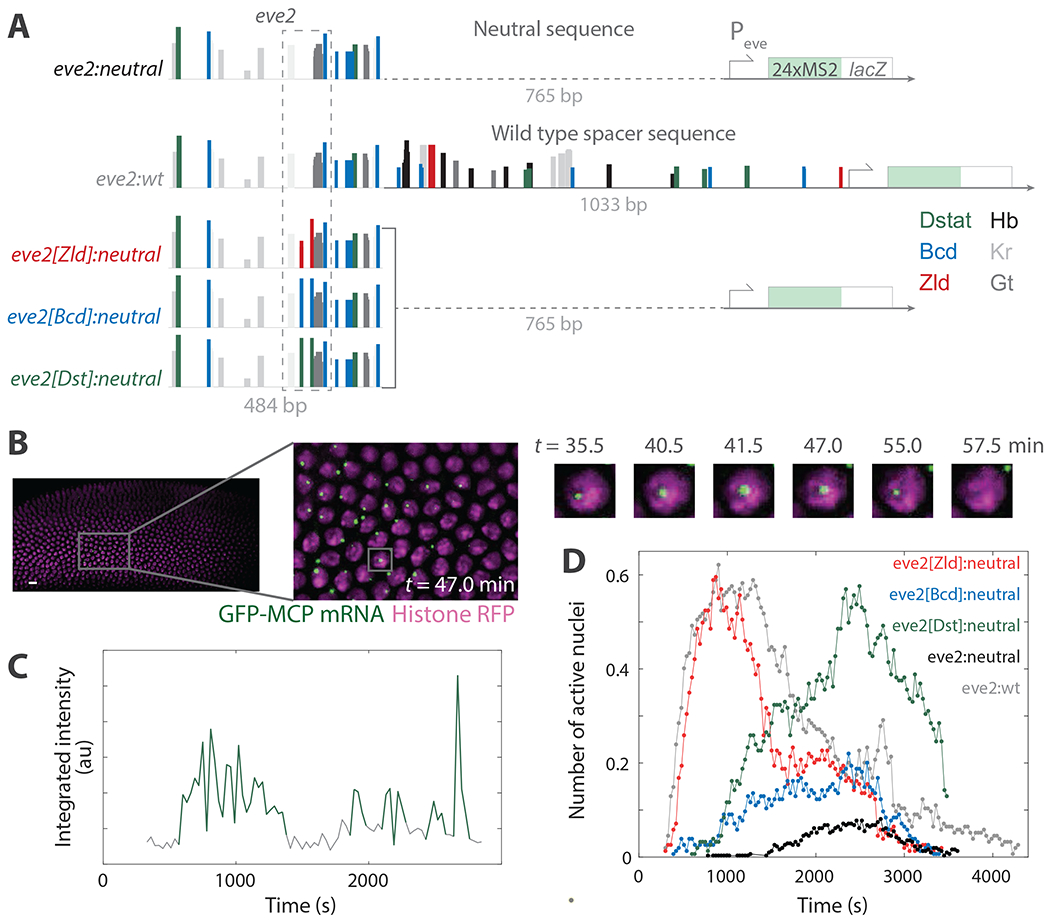
(A) Schematics of the minimal even-skipped stripe two enhancer (eve2) transcription reporter constructs. Each contains the even-skipped promoter driving expression of 24 repeats of the MS2 stem loop sequence followed by a partial sequence of the bacterial lacZ operon. eve2:neutral contains a spacer sequence with no predicted transcription factor binding sites (dashed line). eve2:wt is eve2 with a spacer containing the wild type locus sequence between the enhancer and the promoter. The three transcription factor reporters—eve2[Zld]:neutral, eve2[Bcd]:neutral, and eve2[Dst]:neutral—are identical to eve2:neutral but contain two mutations to add predicted binding motifs for a single transcription activator (dashed box), either Zld, Bcd, or Dstat, respectively. Colored bars are transcription factor binding sites predicted by the software SiteOut ⁶⁰. Hb, Kr, and Gt stand for Hunchback, Kruppel, and Giant, respectively. (B) Left: image of a 2D maximum projection of the diSPIM microscope field of view with histone-red fluorescent protein (magenta) and GFP-MS2 coat protein (green). Gallery images: magnified view of the marked region over time showing a detected active transcription locus. t = 0 corresponds to the beginning of nuclear cycle 14. Scale bar 10 μm. (C) Example MCP-GFP fluorescence emission record from a single nucleus during NC 14. Green marks detected active transcription signal; gray marks intervals during which no fluorescent signal was detected. (D) Dynamic transcription profiles during NC 14 for the constructs in A. Binary detection of the number of detected active transcription loci within the microscope field of view from two replicate experiments for each construct. There are 4535 loci detected across 114 active nuclei for eve2:neutral, 5265 loci from 238 nuclei for eve2:wt, 3631 loci from 289 nuclei for eve2[Zld]:neutral, 1512 loci from 113 nuclei for eve2[Bcd]:neutral, and 4535 loci from 207 nuclei for eve2[Dst]:neutral.

Living embryos were imaged by dual-inverted selective plane illumination microscopy (diSPIM) ⁶⁵. Previous studies have used confocal microscopy ^{33,36,61,66–68}, which relies on oil-immersion objective lenses and requires subjecting the embryos to continuous submersion in halocarbon oil before and during imaging. In contrast, diSPIM relies on water-immersion objective lenses, allowing dechorionated embryos to be placed on a single coverslip and imaged while in a bath of Schneider’s media (Methods). We found that embryos were equally viable when imaged using both techniques ⁶¹. However diSPIM has other advantages, namely decreased photobleaching rates and phototoxicity for a comparable signal-to-noise ratio ^69–71, without loss of spatial or temporal resolution. Here we chose an excitation laser power and image acquisition frequency that did not artificially shorten MCP-GFP signal dwell times through photobleaching as well as minimized any bias towards long dwell times (i.e. did not miss short dwell times; see SFig. 1 and Methods).

We observed the appearance of MCP-green fluorescent protein (MCP-GFP) signal as diffraction-limited spots above background (Fig. 1B). This signal was colocalized with histone-red fluorescent protein (his-RFP) signal, reflecting the binding of many MCP-GFP proteins to nascent RNA in complex with actively transcribing RNA polymerase II proteins (pol II) within individual nuclei ⁷². As in previous studies, we interpreted the appearance of signal from the MBS repeats as the start of active transcription ^67,68,73. When the transcription signal later disappeared, presumably due to transcript termination by most or all actively transcribing pol II and subsequent release of the fluorescently tagged mRNA, this was scored as the end of active transcription.

Scoring genuine active transcription from MS2/MCP records is challenging due to inherent extrinsic noise. We therefore determine instances of active transcription using integrated fluorescence intensity, the size and shape of MS2/MCP signal and hysteresis. To account for size and shape, we assume that actual transcription gives rise to signal that is well-described by a two-dimensional gaussian. We also assume that single frame dropouts (where fluorescence decreases abruptly), are an experimental artifact; we therefore allow for hysteresis in tracking spots to avoid scoring artificially short records. We report binary transcription signal; thus none of the measurements reported here rely on fluctuations in signal intensity. We chose this approach in an attempt to minimize biases that may arise from artifacts that contribute to large fluctuations in MS2/MCP signal intensity. Representative fluorescence intensity records, along with a detailed description of how transcription was scored, are in SFig. 2.

For each imaging replicate, acquisition began during NC 13 and analysis was performed on all time points from the start of NC 14, defined here as the end of anaphase, until the onset of gastrulation. In a comparison of biological replicates, we found the distributions derived from MCP-GFP transcript signal were largely indistinguishable, save for those of eve2:neutral, which drove weaker expression (SFig. 4). For eve2:neutral, no nuclei exhibited MCP-GFP signal above detection threshold until ~20 min into NC 14 (Fig. 1D, black curve), compared to <10 min reported by Bothma et al. for an MS2 reporter driven by eve2 flanked by sequences from the endogenous even-skipped locus. In addition, transcription driven by eve2:neutral was detected in a small number of nuclei compared to that same reporter ⁵⁹. We thus acquired additional replicates of eve2:neutral. All data wrangling and analysis was conducted with custom Matlab software that was in part adapted from an existing platform (⁷⁴; see Code and Data Availability).

Active transcription was not observed outside the stripe 2 pattern during NC 14, except in select cases, wherein transcript signal was detected within the domain of eve stripe 7, which was expected given previous reports that used transcription reporters for eve2 ^59,75–77. The anterior and posterior edges of the stripe 2 domain are set by repressor proteins, including Giant and Kruppel, that bind to sequences within eve2 ^53,78. We limited our analysis to the nuclei located in the center of the stripe (SFig. 3), where these repressive interactions are minimized, in an attempt to isolate activating TF activity from repressive TF activity. Oftentimes, we observed multiple instances of active transcription within the same nucleus (e.g. Fig. 1C, green), consistent with a previous study of eve2 ⁵⁹.

An extended region upstream of even-skipped which includes eve2 drives a normal pattern of expression.

To investigate the cause of the weak expression driven by eve2:neutral, we created a second reporter, eve2:wt, containing a 1517 bp sequence identical to the 5’ region of the endogenous even-skipped locus, composed of eve2 and the 1033 bp sequence between eve2 and the promoter (Fig. 1A). The 1033 bp endogenous sequence contains multiple predicted TF binding motifs, including those for Bcd, Zld and DStat. eve2:wt was also integrated into attP2, and imaged as described above.

In contrast to eve2:neutral, eve2:wt drove early, persistent transcription (Fig. 1D, gray curve) in nearly all the nuclei within the center of the stripe 2 domain (SFig 1). Transcription driven by eve2:wt was detected earlier in the nuclear cycle, occurred in more nuclei, and was more persistent throughout NC 14. This is consistent with a previous study where an MS2 reporter driven by a similar extended version of eve2 was shown to drive a normal pattern of expression ⁵⁹.

Designing regulatory sequences to measure the activity of individual TFs.

Our strategy to measure the kinetic roles of different activating TFs was to add binding sites for those TFs to an enhancer scaffold, and measure the resulting differences in expression. This required a scaffold where the consequences of additional activation are not obscured by a high baseline of transcription signal. In previous studies, high levels of activity were thought to obscure the detection of transcriptional bursts ^36,67,68. The eve2:neutral reporter, with its weak basal expression, provides this scaffold. We therefore created a set of variants of eve2:neutral designed to recruit additional specific TFs to the reporter. For each variant, we introduced two DNA binding motifs for a single TF—either Zld, Bcd, or Dstat—by making two short sequence mutations (8 to 10 nucleotides) in the same location in eve2, chosen to minimize disruption to other TF binding sites (See Methods). Each of these activating TF reporters—eve2[Zld]:neutral, eve2[Bcd]:neutral, and eve2[Dst]:neutral—were incorporated into attP2 and imaged as above (Fig. 1A). Note that eve2:wt acts as an approximation of the upper-bound for transcription activation by eve2:neutral and its variants, and is therefore an informative benchmark for qualitative comparisons. However, all quantitative comparisons that follow are between eve2:neutral and its variants, the TF reporters.

All three of the TF reporters induced transcription that exceeded that of eve2:neutral. Each dramatically altered the dynamic transcription profile (Fig. 1D) and did so in a unique way. eve2[Bcd]:neutral induced transcription similar to that of eve2:neutral, but earlier and in a greater number of nuclei. eve2[Dst]:neutral and eve2[Zld]:neutral also induced transcription earlier than eve2:neutral but in far more nuclei, similar to that of eve2:wt. However, the timing of activation by eve2[Dst]:neutral and eve2[Zld]:neutral was different. The dynamic transcription profile of eve2[Zld]:neutral peaked early in the nuclear cycle then decayed quickly, again similar to eve2:wt, while that of eve2[Dst]:neutral had a later, broader peak. To make quantitative comparisons between the TF reporters, we employed a collection of simple empirical models, as described in the next section.

Empirical kinetic models distinguish the roles of Zld, Bcd and Dstat in regulating transcription.

We analyzed the transcription records for eve2:neutral and each TF reporter, and report the distributions of three different measurements—the first passage time, the active transcription lifetime, and the idle period—which we explain below. These MS2/MCP measurements are straightforward and their distributions are simple to extract from any live imaging dataset (see Discussion). To analyze the shape of these distributions, and to compare across constructs, we used models commonly employed in the analysis of single molecule data. These models produce characteristic distributions and we asked how well they fit our data ⁷⁴. Multiple models were compared to each experimental distribution and adequate fit was assessed by how well the features of the experimental distribution were reproduced by the model. Adequate fits yield a set of parameters that we compare between constructs to assess the ways in which the kinetic roles of these TFs are similar or different. However, we emphasize that the absolute values of these parameters are not necessarily informative, but their values relative to one another are. Because the number and affinity of binding sites for each of Zld, Bcd, and Dstat differs within eve2, we made direct comparisons between each TF reporter and eve2:neutral.

First passage times

There are dramatic differences in the dynamic transcription profiles of the TF reporters at early time points (Fig. 1D). These differences are represented in the distributions of first passage times, when transcription is first detected in each nucleus in NC 14 (Fig. 2). These distributions have three important features related to the mechanisms that lead to first passage into transcription. First, the maximum slope of the distribution is related to the rate of initial transcription activation across the stripe pattern. Second, the plateau of the distribution is the fraction of active nuclei within the stripe. Third, the time delay between the end of anaphase (i.e. t = 0 in Fig. 2B) and the first detection of transcription within the stripe 2 domain (e.g. Fig. 2B t = 300 s and t = 1260 s for eve2:wt and eve2:neutral, respectively) is related to the number and length of kinetic states that regulatory DNA must pass through prior to reaching a state capable of initiating transcription.

Figure 2. First passage activation kinetics.

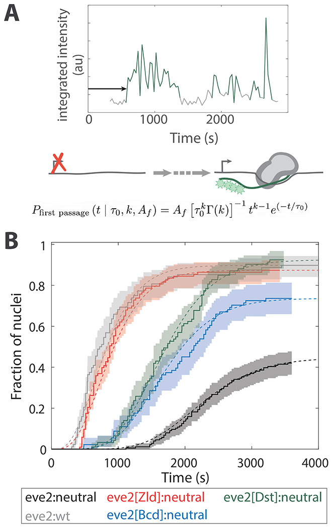
(A) Graphical depiction of a first passage into transcription measurement. Emission record as in Fig. 1C. The arrow denotes the first passage time for this nucleus. Cartoon: during this interval the transcription reporter transitions from a state incapable of activating transcription (left), through a number of rate limiting steps (dashed arrow ), to a transcriptionally competent one that activates transcription (right). The mathematical model (Eq. 1) is shown at the bottom. (B) Cumulative first passage distributions (solid curves) overlaid with a model (Eq. 1, dashed curves) with the characteristic number of rate limiting steps, $k$, a characteristic time constant for each of those steps, ${\tau }_0$, and the fraction of active nuclei within the center of the stripe, $A_f$; see Table 1 for parameter values. The curves are normalized to the total number of nuclei in the center of the stripe (see SFig. 3). There were 74 active nuclei and 166 nuclei total in the center of the stripe for eve2:neutral; 79/88 nuclei were active in the center of the strip for eve2:wt; 90/103 for eve2[Zld]:neutral; 67/91 for eve2[Bcd]:neutral; 86/93 for eve2[Dst]:neutral. Shaded regions represent the 90% confidence intervals from bootstrapping methods (see Methods).

Choosing a model to describe the first passage distributions has been challenging for researchers working with MS2/MCP data ^30,33,39. One approach has been to ignore the time delay following the end of anaphase and only consider the first passage times once transcription has been detected in any nucleus across the entire pattern (as in ³³). This is reasonable since transcription cannot take place during mitosis—a process called mitotic repression ^79,80. We initially ignored the time delay and attempted to apply the same models that are used to describe single molecule kinetics ⁷⁴. These models performed poorly. However, they taught us that the observed first passage distributions cannot be explained by a kinetic pathway with less than 3 transcriptionally silent, rate limiting steps (explained in SFig. 5). In addition, note that the time delay varies by ~900 s between the five different reporters (Fig. 2B). This is difficult to reconcile with the general mechanism of mitotic repression, which would act similarly across reporters. These data suggest that TFs are acting to shorten this time delay (see Discussion). We therefore employed a model that can accommodate both of these observations. Namely, more than two transcriptionally silent slow steps and highly variable time delays following mitosis.

A critical choice for implementing this type of model concerns the characteristic time constants associated with each transcriptionally silent step. Although it is unlikely that they are all equivalent, it is reasonable to assume that they are each of the same order of magnitude ^2,23. We chose to assume the time constant of each silent step is equal. This decision was made for a couple of reasons. First, it kept the number of free parameters lower than a model which allowed the rate of each silent step to vary independently. Second, we had little a priori evidence of what, biologically, these silent steps might represent and what their cognate rates might be. Finally, this choice aligns with previous studies ^30,33. From this, we are forced to assume that the number of rate limiting steps must change to account for the differences in the first passage distributions in Fig. 2B. This is not to say that the kinetic pathway itself changes, only that under different circumstances some steps become fast and are no longer rate limiting. Finally, due to the limitations of the perturbations here, the model must be agnostic to exactly what the rate limiting steps represent biochemically and the order in which they occur. We discuss other modeling options in the Discussion.

From these choices, we arrived at a linear kinetic model of several steps, each with an equivalent characteristic time constant. Each step is assumed to be irreversible. This simplifying assumption is likely not appropriate for every step in the kinetic pathway, but, mathematically, the mean rate of transcription from any linear kinetic scheme containing reversible steps can be substituted by an equivalent scheme of irreversible steps through the addition of pseudo-steps that do not represent biochemical reactions (Scholes et al., 2016). Therefore, the qualitative conclusions here will likely be unchanged even if the true kinetic scheme contains reversible steps. And we emphasize that our question is simply whether the kinetic roles of individual TFs are distinguishable; this does not require strict interpretation of the actual values of the parameters, only their relative values.

Statistical assessment of error for this and other models was assumed to lie at the level of individual nuclei and not at the level of individual embryos. This approach is common with data from single nuclei ⁸¹. This assumption is reasonable, considering that within the same nucleus transcription from two alleles of the same gene are not strongly correlated ⁸². In addition, we have i. limited the analysis to a narrow region within the center of the stripe 2 pattern (SFig. 3), where the extra-nuclear environment is similar, and ii. limited the measurements that we report to those which do not obviously suffer from embryo-to-embryo variability, such as pattern border location ⁸³. This strategy fortuitously confers the statistical power of many independent measurements (i.e. nuclei) onto these data, rather than a few (i.e. embryos; see Methods and SFig. 4).

We described the first passage distributions with a gamma distribution model (a generalization of the Poisson distribution):

$$P_{\text{first passage}}^i\left(t|{\tau }_0,k^i,A_f^i\right)=A_f^i{\left[{\left({\tau }_0\right)}^{k^i}\text{Γ}\left(k^i\right)\right]}^{-1}{t}^{k^i-1}\mathit{\text{exp}}\left(-t/{\tau }_0\right)$$ Eq. 1

Where $i$ ≡ eve2:wt, eve2:neutral, eve2[Zld]:neutral, eve2[Bcd]:neutral, or eve2[Dst]:neutral. $A_f$ is the active fraction of nuclei in the center of the stripe, ${\tau }_0$ and $k$ are the gamma distribution scale parameter and shape parameter, respectively, and $\mathrm{\Gamma }$ is the gamma function (Fig. 2B, smooth curves; Table 1). Gamma distributions have been applied in a wide variety of contexts in biology, for example, to determine the mechanism of molecular motors from single molecule data ⁸⁴. Dufourt et al. did so for measurements similar to those in Fig. 2 ³³. $k$ can be interpreted as the average number of rate-limiting steps, while ${\tau }_0$ can be interpreted as the characteristic time constant of each of these steps. Here, we chose to fit the time constant, ${\tau }_0$, globally to all five reporter data sets while simultaneously fitting the number of steps, $k$, independently for each reporter construct (see Methods for an explanation of this choice).

Table 1. First passage into active transcription model parameters.

See Eq. 1. The characteristic lifetime for all rate limiting steps, ${\tau }_0$, was globally fit to all five transgenic reporters. Standard errors were computed using bootstrapping methods (see Methods).

	$A_f$	$k$	${\tau }_0$
eve2:neutral	0.45 ± 0.04	11.3 ± 1.2	205 ± 20 s
eve2:wt	0.90 ± 0.03	4.1 ± 0.4
eve2[Zld]:neutral	0.87 ± 0.04	4.4 ± 0.5
eve2[Bcd]:neutral	0.74 ± 0.05	8.5 ± 1.0
eve2[Dst]:neutral	0.92 ± 0.06	8.5 ± 0.9

From the model, the first passage distributions can be explained by a varying number of rate limiting steps, each with a characteristic time of 205 ± 20 s. Each of the activating TF reporters increased the active fraction of nuclei within the stripe relative to eve2:neutral ($A_f$ in Table 1). This quantifies what would be expected from inspection of the dynamic transcription profiles in Fig. 1D. In addition, all reporters decreased the number of rate limiting steps relative to eve2:neutral: $k$ = 11.3 ± 1.2 for eve2:neutral, 8.5 ± 1.0 and 8.5 ± 0.9 for eve2[Bcd]:neutral and eve2[Dst]:neutral, respectively, and 4.1 ± 0.4 and 4.4 ± 0.5 for eve2:wt and eve2[Zld]:neutral, respectively. Regardless of the detailed interpretation of this model, it is clear that while all reporters reduce the number of rate limiting steps on the path to first passage transcription activation, those that bind Zld (eve2:wt and eve2[Zld]:neutral) do so to a large extent. This explains much of the differences in the dynamic transcription profiles of Fig. 1D, but not entirely. The TF reporters must be acting to tune other kinetic parameters in addition to the first passage time.

Active transcription lifetimes

An active transcription lifetime is the time over which signal is continuously detected within a single nucleus (Fig. 3A). This value is proportional to the number of RNA molecules synthesized during that time interval ⁵⁹. The cumulative distributions in Fig. 3B show the survival of the active transcription lifetimes. The rate at which these curves fall off for increasing active transcription dwell time (i.e. the slope) is proportional to the rate by which active transcription turns off (see Methods).

Figure 3. Active transcription and idle period kinetics.

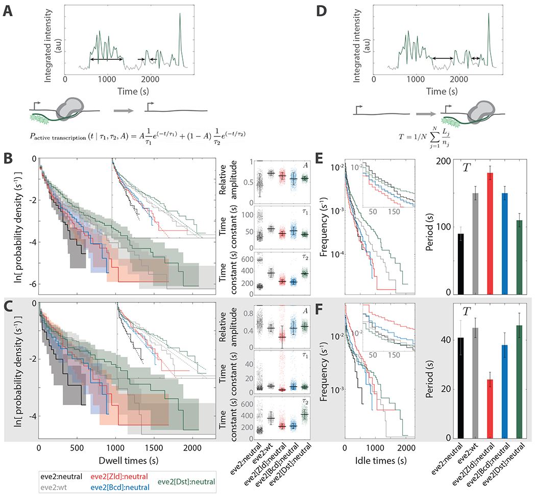
(A) Graphical depiction of active transcription lifetime measurements. The double headed arrows denote two example intervals of active transcription. Cartoon: during these intervals the reporter locus transitions from a state containing many RNA polymerase molecules (gray bean) undergoing RNA synthesis (green line) to one lacking detectable active transcription (green stars). The model (Eq. 2) is shown at the bottom. (B) Cumulative lifetime distributions of active transcription (solid curves). $n=\mathrm{190,\; 507,\; 363,\; 236}$, and 444 for eve2:neutral, eve2:wt, eve2[Zld]:neutral, eve2[Bcd]:neutral, and eve2[Dst]:neutral, respectively. Data is overlaid with a model (Eq. 2; dashed curves). Shaded regions represent 90% confidence intervals from bootstrapping methods using 10,000 simulated datasets (Methods). The mean and standard error of the model parameters, time constants ${\tau }_1$ and ${\tau }_2$ and relative amplitude $A$, are to the right. These plots also show 1,000 randomly selected parameter sets from fitting Eq. 2 to simulated data from bootstrapping (points). The bi-modal nature of the eve2:neutral parameter values is due to simulated data frequently lacking a substantial long-lived population, making those distributions best characterized solely by the ${\tau }_1$ parameter (with $A=1$). (C) As in B, but the data have been partitioned into the 20% of active transcription lifetimes that first appear during NC 14 (see Methods). n = 37, 104, 75, 51, and 89 for eve2:neutral, eve2:wt, eve2[Zld]:neutral, eve2[Bcd]:neutral, and eve2[Dst]:neutral, respectively. (D–F). Idle transcription period. (D) Graphical depiction of idle transcription period measurements. The double headed arrows denote two idle periods. Cartoon: during these intervals the transcription reporter locus transitions from a state lacking active transcription to one containing many RNA polymerase molecules undergoing RNA synthesis. The model (Eq. 3) is shown at the bottom. (E) Cumulative frequency distributions of the idle periods (left). The inverse of the mean idle period, in units of s⁻¹, can be read directly from these distributions via the vertical axis intercept (inset); these, along with their standard error, are depicted on the right. See Table 3. n = 116, 428, 273, 169, and 358 for eve2:neutral, eve2:wt, eve2[Zld]:neutral, eve2[Bcd]:neutral, and eve2[Dst]:neutral, respectively. (F) As in E, but for the 20% of idle periods that first occur during NC 14.

These curves can reveal one or more types of activation present in the distribution, each type defined by a characteristic lifetime ⁷⁴. For example, the distributions in Fig. 3B do not reflect the presence of a single characteristic lifetime (SFig. 6). They are not straight but kinked; the kink separates two regions of the curves, each with a distinct slope. This led us to a apply a bi-exponential probability density function, which is commonly used to describe chemical kinetics (e.g. ¹⁵), to model these distributions:

$$P_{\text{active transcription}}^i\left(t|{\tau }_1^i,{\tau }_2^i,A^i\right)=A^i\frac{1}{{\tau }_1^i}{e}^{\left(-t/{\tau }_1^i\right)}+\left(1-A^i\right)\frac{1}{{\tau }_2^i}{e}^{\left(-t/{\tau }_2^i\right)}$$ Eq. 2

Where ${\tau }_1$ and ${\tau }_2$ are characteristic lifetimes, $A$ and $1-A$ are the relative amplitudes of each, respectively (Fig. 3B, smooth curves). These parameters were determined by maximum likelihood fitting to the distributions of active transcription lifetimes (Table 2; see Methods). The slope of the model over short lifetimes is proportional to the inverse of a short-lived characteristic time, ${\tau }_1$, and the slope at longer dwell times is proportional to the inverse of a second, longer-lived characteristic time, ${\tau }_2$. In other words, once activated, for both eve2:neutral and eve2:wt, transcription does not turn off stochastically with a single characteristic lifetime.

Table 2. Model parameters values for active transcription.

See Eq. 2. Early lifetime distributions are composed of the first 20% of active transcription intervals detected for each reporter. Later distributions are composed of the other 80%. Standard errors were computed using bootstrapping methods.

		$A$	${\tau }_1$	${\tau }_2$
All lifetimes	eve2:neutral	0.43 ± 0.12	36 ± 8 s	140 ± 20 s
	eve2:wt	0.71 ± 0.05	59 ± 7 s	370 ± 50 s
	eve2[Zld]:neutral	0.65 ± 0.09	45 ± 8 s	230 ± 40 s
	eve2[Bcd]:neutral	0.58 ± 0.12	53 ± 14 s	220 ± 40 s
	eve2[Dst]:neutral	0.59 ± 0.04	42 ± 5 s	360 ± 40 s
Early lifetimes	eve2:neutral	0.56 ± 0.12	34 ± 10 s	200 ± 50 s
	eve2:wt	0.48 ± 0.07	45 ± 10 s	500 ± 70 s
	eve2[Zld]:neutral	0.26 ± 0.16	22 ± 7 s	310 ± 60 s
	eve2[Bcd]:neutral	0.47 ± 0.12	41 ± 16 s	320 ± 60 s
	eve2[Dst]:neutral	0.51 ± 0.08	39 ± 9 s	600 ± 120 s
Later lifetimes	eve2:neutral	0.38 ± 0.27	34 ± 12 s	120 ± 40 s
	eve2:wt	0.78 ± 0.10	63 ± 12 s	280 ± 80 s
	eve2[Zld]:neutral	0.68 ± 0.15	44 ± 10 s	150 ± 50 s
	eve2[Bcd]:neutral	0.48 ± 0.24	48 ± 17 s	160 ± 50 s
	eve2[Dst]:neutral	0.56 ± 0.06	40 ± 5 s	270 ± 30 s

Kinetically, each of these two types of activation represent a state of the system, each of which contribute to both terms in Eq. 2 . The exact details of the biochemical identities, stability, and pathways of these states cannot be determined from the data and analysis here.

The model in Eq. 2 revealed the kinetic differences between activation by eve2:wt and activation by eve2:neutral. The apparent increase in transcription driven by eve2:wt was due to longer characteristic times, ${\tau }_1$ and ${\tau }_2$, as would be expected a priori. However, an interesting wrinkle emerged from the application of the model. The fraction of long-lived lifetimes, $(1-A)$, was greater for eve2:neutral. eve2:wt drove greater transcription than eve2:neutral, but it did so while activating, proportionally, more frequent short lifetimes.

The bi-exponential nature of the active transcription lifetimes was unexpected. We hypothesized that this reflects a change of the gene regulatory network over time, and therefore characteristically longer active lifetimes only occur early in NC 14. To test this, we divided the active lifetime measurements of Fig. 3B into two subsets: those that first activated early in NC 14 and those that first activated later (Fig. 3C and SFig. 7, respectively; see Methods). We applied the model in Eq. 2 to each of the two subset distributions (early and later) of eve2:wt and eve2:neutral. These subsets yielded characteristic lifetimes, ${\tau }_1$ and ${\tau }_2$, similar to those of the whole distributions (Table 2). However, the relative amplitudes, $A$ and $1-A$, were different. In each case, the relative amplitude for the early distribution was dominated by long-lived activations (i.e.$(1-A)>A$). For eve2:wt, the amplitude of long-lived activations for the early distribution was $1-A^{\text{eve}2:wt,\mathit{\text{early}}}=0.52\pm 0.10$, up from $1-A^{\mathit{\text{eve2:wt}}}=0.29\pm 0.05$ for the whole distribution. For eve2:neutral the long-lived amplitude was $1-A^{\mathit{\text{eve2:neutral}},\mathit{\text{early}}}=1.00\pm 0.12$ for the early subset, compared to $1-A^{\mathit{\text{eve2:neutral}}}=0.57\pm 0.12$ for the whole distribution. The bi-exponential nature of these distributions cannot entirely be attributed to a hand-off between gene regulatory networks over the course of NC 14 (see Discussion).

We determined how additional activity of Zld, Bcd and Dstat in the TF reporters affected the characteristic active lifetimes by applying the model in Eq. 2 to their respective distributions (Fig. 3B). This revealed that only eve2[Dst]:neutral displayed active lifetime kinetics that were different from eve2:neutral (Table 2). Most notably, eve2[Dst]:neutral induced longer long-lived active times (${\tau }_2^{\mathit{\text{eve2[Dst]:neutral}}}>{\tau }_2^{\mathit{\text{eve2:neutral}}}$). When these distributions were divided into early and later subsets, this trend held up for the later active lifetime distributions (SFig. 7, Table 2). However, for the subset of early active times, all three activator reporters showed an increase in the characteristic lifetime for long-lived active times, ${\tau }_2$ (Fig. 3C, Table 2). Two conclusions can be drawn. First, the TF reporters increase active lifetimes by altering the long-lived characteristic time, ${\tau }_2$, and not the short-lived characteristic time, ${\tau }_1$, nor the fraction of long-lived events, $1-A$. Second, at any given time point during NC 14, more nuclei will be undergoing active transcription for each of the activating TF reporters compared to eve2:neutral. The modulation of the active transcription lifetime therefore meaningfully contributes to the differences in the dynamic transcription profiles of Fig. 1D.

Idle transcription

We define idle transcription as the interval of time between the end of one observed active transcription interval and the beginning of the next within the same nucleus (Fig. 3D, SFig. 8, 9). During these intervals, the MCP-GFP transcription signal was below the detection threshold. Analogous to a car engine that idles while waiting at a stop light, transcription may still be occurring during these periods, but at a level that we could not detect. As with active transcription lifetimes, idle periods are related to the number of transcripts synthesized over NC 14; decreasing the idle period increases the total time over which a locus is actively transcribing. Modulating the length of idle periods in a time-dependent fashion can regulate when and how much of a transcript is produced.

We attempted to describe the idle period distributions with a kinetic model similar to the model that was used to describe the active transcription distributions (SFig. 9). This attempt was unsuccessful, but informative. Both the shape of the distributions (SFig. 9B) and the model parameter values (SFig. 9C) indicated that a single exponential model was the best characterization of the data (explained in SFig. 9). The characteristic time constant of a single exponential distribution is the mean of that distribution. Accordingly, we chose to use the mean idle period to make comparisons.

The mean idle period is:

$$T^i=1/N^i\sum _{j=1}^{N^i}\frac{L_j^i}{n_j^i}$$ Eq. 3

Where N is the total number of nuclei with at least one detected active transcription interval, L is the cumulative length of time during which no transcription signal was detected in these same nuclei (see SFig. 8), and n is the number of active transcription lifetimes (of any length) observed in these nuclei.

When considering the entirety of nc14, the mean idle period increased for each of the TF reporters when compared to eve2:neutral (Fig. 3E). These results likely do not represent meaningful biological conclusions; because eve2:neutral turns on transcription so late in the nuclear cycle, there is little opportunity for long idle periods to occur before the onset of gastrulation (SFig. 8). Thus, eve2:neutral drives short idle periods and all TFs appear to increase idle periods in comparison. However, when analyzing idle periods that take place just after a nucleus turns on (see Methods), eve2[Zld]:neutral showed a significant decrease in mean idle period relative to eve2:neutral , while eve2[Bcd]:neutral and eve2[Dst]:neutral showed no significant effect (Fig. 3F).

DISCUSSION

Our goal was to determine the kinetic roles of three different TFs known to activate transcription in the Drosophila blastoderm embryo. We measured their effects on transcription in living embryos using a set of transcription reporters wherein variants of eve2 drive MCP-GFP marked nascent transcripts, and contextualized our measurements using models derived from chemical kinetics. We characterized two benchmark reporters that served as effective lower- and upper-bounds for each measure of transcriptional activity, which allowed us to discern the effect of individual TFs by comparison. Straightforward inspection of the data yielded qualitative insights into roles for the three TFs: Zld, Bcd, and Dstat. Quantitative analysis with our empirical models provided additional insight by contrasting the probability distributions of first passage activation times, active transcription lifetimes, and idle periods associated with each transgenic reporter. We found that the active transcription lifetime and mean idle period changed over time, with longer activation lifetimes as well as shorter idle periods early in nuclear cycle 14. We further found that each TF drove transcription in kinetically distinguishable ways, as summarized in Fig. 4 and discussed in more detail below. Our results support the feasibility of kinetic synergy in eukaryotic gene regulation. Our results also highlight unresolved questions, including how TFs bound outside of canonical enhancers affect transcriptional output and how different combinations of TFs can achieve similar transcription output.

Figure 4. Kinetic roles of three transcriptional activators.

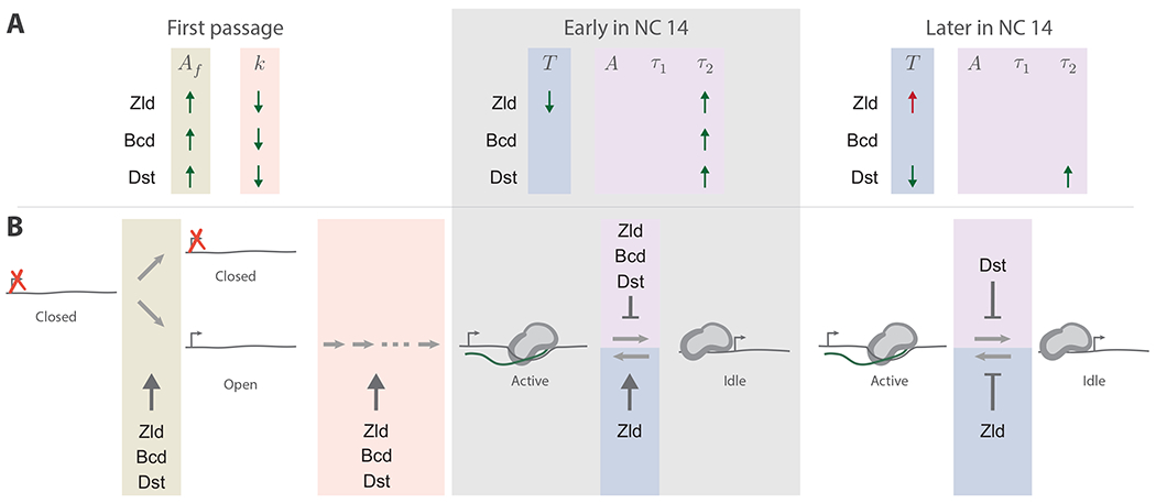
(A) A graphical summary of the impact of each TF on each kinetic parameter. The arrows denote if a parameter is increased or decreased by a TF. Parameter changes consistent with activation (i.e. lead to more transcription) are shown in green and changes consistent with repression in red. Beige and peach mark the first passage transcription model parameters (Eq. 1), blue marks the mean idle period (Eq. 3), and purple the active transcription model parameters (Eq. 2). The gray shaded region denotes active and idle parameters early in NC 14. (B) Model of transcription and its regulation during NC 14. Colored regions are as in A. All three TFs increase the fraction of active nuclei (arrow in beige region), and they decrease the number of steps to first passage transcription (arrow in peach region). At different times during NC 14, the TFs promote active transcription by suppressing the transition from the active to the idle state (T-bars in purple regions). Early in NC 14, Zld increases transcription by increasing the rate into the active state from the idle state, while Dst does so later (arrows in blue regions). Zld decreases this same rate later in the NC 14 (T-bar in blue region). The ellipsis represents a variable number of rate limiting steps on the pathway to first passage transcription.

Insights into transcriptional kinetics

Inferring kinetic roles from dynamical data requires a mathematical model. To date, there are several examples of studies that use math models to describe MS2/MCP experiments (e.g. ^30,40,85). These models assumed a kinetic scheme, typically composed of two states, then attempted to measure transitions between or probability of these states. This “forward theory” approach has the potential to realize the rate limiting steps of regulation and will be essential to understanding how proteins and nucleic acids collectively give rise to transcription regulation ^86,87. Unfortunately, these models are often phenomenological, given our lack of ability to directly measure most biochemical steps of eukaryotic transcription. “Reverse theory” (e.g. empirical theory), while lacking the predictive power of forward theory, nonetheless has provided mechanistic insight into molecular interactions and regulatory concepts. Here, we argue that when the underlying kinetic scheme cannot be explicitly perturbed and may be “hideously complicated,” an empirical approach makes “good sense” ⁸⁷. While this approach contains certain assumptions, like any other, its power stems from a lack of assumptions about the underlying kinetics, mitigating concerns around the correctness of the model.

The models used here are agnostic to the underlying biochemical states of the transcriptional system. In effect, we are summarizing the kinetics of transcription signals by using empirical models to describe probability distributions. The time constants reported here are related, but not identical, to the underlying kinetic pathway of transcription. This is in contrast to other studies that have attempted to measure kinetics of nascent transcription in embryos by using forward theory by assuming an underlying kinetic model. For example, Xu et al. assumed a two state model of transcription, then extracted the rates between the states by fitting their model to distributions of nascent transcripts as measured in fixed embryos using single molecule FISH ⁸¹. Lammers et al. also assumed an underlying two state model, then measured transitions between them by inferring the state of the system from the intensity record of a fluorescent MS2/MCP reporter ⁴⁰.

In this work, we sought to quantify how dynamic transcriptional outputs changed with increased Zld, Bcd, and Dstat activity; our goal was to ask whether these three TFs had kinetically distinguishable roles. This goal had the advantage of not requiring any assumptions about the kinetic scheme a priori. It only requires precisely characterizing differences in transcriptional outputs. Our approach has well established methods for its application ^74,88 and relies on a simple binarization of MS2/MCP data (Methods). It is broadly applicable to all live imaging transcription studies.

Our analysis was restricted to the distributions of first passage activation times, active transcription lifetimes, and idle periods. Other distributions, including fluorescence intensity (signal brightness) and intensity fluctuations (noise), were not included due to the dependency of these measurements on experimental conditions that are difficult to control. These include excitation laser drift and day-to-day variability, heterogeneous illumination across the field of view of the microscope, nucleus-to-nucleus variation in the depth of the reporter gene relative to the surface of the embryo, and photobleaching of GFP fluorophores over the course of an experiment. All of these sources of extrinsic noise bias fluorescence intensity measurements and must be accounted for when reporting those distributions. These variables can and should be controlled for to the extent that they can be (e.g. SFig. 1). However, because we largely eschew measures of signal intensity, the approach laid out here is robust against them.

One notable result from this study is the large differences in the time delays between the end of anaphase and the first detection of transcription (Fig. 2). These differences strongly suggest that the regulation of the rates of first passage transcription is an important and widespread mechanism of activating TFs. From qualitative inspection, each of the activating TFs reduced this delay, and they did so dramatically (Fig. 1D). Our modeling approach further supported this observation, and showed that each TF increased the active fraction of nuclei, which had previously been shown to be important for patterning in the embryo ^40,67. In addition, our model showed that each TF also decreased the number of rate limiting steps, $k$. It is worth noting that these data are also consistent with a model wherein each TF lowers the time constant of each of several consecutive rate limiting steps (this can be shown by globally fitting $k$ while fitting ${\tau }_0$ to each construct individually, see Methods). In either case, each TF is implicated in regulating the kinetic steps that lead to the onset of transcription, and not just the likelihood that a locus ever turns on.

To our knowledge, this is the second report of a bi-exponential probability distribution of active lifetime MS2/MCP measurements. Darzacq et al., using photoactivated MS2/MCP in cultured human cells, reported characteristic time constants (~33 s and ~250 s of the same order of magnitude as those we report here ⁸⁹. As noted above, this implies that two stable states of the system exist. However, what, biologically, these two stable states represent is not clear.

The short time constants reported here, ${\tau }_1$, match well to the time we predict a pol II molecule to process along the reporter gene used in these experiments. Recent reports of pol II elongation rates in the fly blastoderm range from 40 - 50 bp/s ^40,73. Here the DNA template is ~3400 bp from the end of the MS2 stem loop cassette to the poly A termination signal. Assuming MCP-GFP binds quickly following stem loop synthesis and the nascent transcript is released quickly from the site of termination, a nascent transcript would be fluorescently tagged and colocalized with the gene locus for around 75 s, which is somewhat consistent with the ${\tau }_1$ values reported here, 22 to 63 s. One interpretation supposes that the short-lived instances of transcription represent low level stochastic initiation, wherein up to a handful of pol II molecules are able to initiate, elongate, and terminate together in succession before initiation is once again ceased. The frequency and duration of these instances is minimally impacted by TFs in this context.

Significant differences between the active lifetime distributions were almost entirely attributable to changes in the long-lived characteristic lifetime, ${\tau }_2$ (Fig. 3B, Table 2). This parameter ranges from 140 - 600 s, which is longer than the ~75 s we might expect for synthesis of a single transcript. During elongation, pol II processes at highly variable rates ⁹⁰ and can enter paused states far downstream of the promoter ⁹¹. It is possible that these mechanisms lead to pol II traffic jams on the gene, leaving fluorescently tagged elongation complexes paused or arrested at the gene. The long-lived state that we observed may represent these instances, as was proposed by ⁸⁹. In our data, each TF, at one time or another, dramatically increased the long-lived transcription lifetimes (Fig. 4), suggesting the long-lived state represents a highly regulated state/s, wherein many pol II molecules successively initiate transcription and process over a time window lasting several hundred seconds.”

This work also showed that a stripe enhancer, eve2, isolated from the other enhancers in the eve locus loses the ability to drive expression as NC 14 progresses (Fig. 1D, gray curve), despite the fact that the TFs that regulate eve2 remain present. This type of “enhancer shut-down” is widespread in developmental networks; many developmental genes are controlled by multiple enhancers (often called shadow enhancers) and the regulation of these genes can transition from one enhancer to another as development progresses (e.g. ^61,92). In the Drosophila embryo, there are three different gene regulatory networks active over NC 14 which drive expression of the seven pair-rule genes, including eve. The transition between these gene regulatory networks is marked by a change in enhancer dependence ⁹³. However, the mechanisms of enhancer shut-down and/or hand-off between enhancers is not currently known. Our modeling revealed that the kinetic role of a TF can change over time (Fig. 4), and we speculate that mechanisms of enhancer shutdown are related to the changing roles of TFs at individual genes. For example, some TFs initially have kinetic roles that lead to greater transcription, while later they have roles that lead to reduced transcription, as discussed below. Exploring this process of enhancer shutdown is poised to be an emerging topic in developmental biology.

Insights into TF function

Zld is thought to act as a pioneer factor in the embryo, opening chromatin and maintaining it in a state competent for transcription ^94–96. Kinetically, it is reasonable to hypothesize that this mechanism would decrease the number of rate limiting steps to first passage transcription. Consistent with this, we found that in this context Zld dramatically decreased the number steps, $k$. However, Zld also affected other kinetic parameters (Fig. 4). Zld increased transcription by increasing active transcription lifetimes, ${\tau }_2$, but only for early times in the nuclear cycle. Also, Zld increased transcription early in the nuclear cycle by decreasing the idle period, $T$ (Table 3). Zld has been shown to perform multiple roles at different target genes ^30,33, but to our knowledge, this is the first evidence that it plays multiple roles at a single gene over time.

Table 3. Mean idle transcription periods.

See Eq. 3. Early idle times are the first 20% detected for each reporter. Later idle times are the other 80%. Standard errors were computed using bootstrapping methods.

		T
All periods	eve2:neutral	89 ± 8 s
	eve2:wt	152 ± 7 s
	eve2[Zld]:neutral	176 ± 9 s
	eve2[Bcd]:neutral	149 ± 10 s
	eve2[Dst]:neutral	108 ± 5 s
Early periods	eve2:neutral	41 ± 7 s
	eve2:wt	45 ± 4 s
	eve2[Zld]:neutral	24 ± 3 s
	eve2[Bcd]:neutral	38 ± 5 s
	eve2[Dst]:neutral	46 ± 5 s
Later periods	eve2:neutral	81 ± 6 s
	eve2:wt	159 ± 7 s
	eve2[Zld]:neutral	183 ± 10 s
	eve2[Bcd]:neutral	155 ± 11 s
	eve2[Dst]:neutral	110 ± 6 s

Two Zld binding site insertions served to turn the dynamic transcription profile of eve2:neutral into something close to that of eve2:wt (Fig. 1D). From this qualitative observation, one might conclude that the similarity is due to a similar number of Zld binding motifs in both eve2[Zld]:neutral and eve2:wt (see the sequence schematics in Fig. 1A), even though regulatory sequences can be sensitive to binding motif position, orientation, and neighboring sequences ^56,97. However, our modeling does not support this interpretation. Following first passage into active transcription, eve2:wt maintained active transcription by increasing the active transcription lifetimes, ${\tau }_2$, relative to eve2:neutral over all of NC 14. Zld did so by increasing ${\tau }_2$, and decreasing the mean idle period, but only for early times in the nuclear cycle. Zld then repressed transcription later on by increasing idle periods in nuclei that were previously active. Therefore, the similarity between the eve2[Zld]:neutral and eve2:wt dynamic transcription profiles cannot entirely be attributed to Zld activity as the two regulatory sequences produce similar spatiotemporal outputs by acting on different combinations of kinetic parameters.

Bcd is a highly studied TF, with considerable focus placed on how the Bcd gradient and cooperative interactions between Bcd proteins regulate target genes ^{44,45,48,98–100}. Our characterization of kinetic roles found that Bcd, in this context, increased the active fraction of nuclei and decreased the number of rate limiting steps to first passage transcription. This is, perhaps, consistent with a previous report of Bcd activity early in the nuclear cycle and its capacity for pioneering activity (Hannon et al., 2017). However, early in the nuclear cycle, Bcd displayed both activating and repressing kinetic roles by suppressing both the transition out of the active state as well as the transition into it (Fig. 4). Later in the nuclear cycle, Bcd had no significant impact on the kinetics of transcription. This may be unsurprising, given another report that Bcd is a bifunctional transcription factor in certain contexts ¹⁰¹, but the activating/repressing activities of Bcd reported here are different than the bifunctional regulation previously reported. In this work, Bcd acts to tune different parameters at different times during the nuclear cycle, sometimes resulting in an increase in the number of transcripts synthesized, and other times resulting in a decrease. Although intriguing, these conclusions should be treated with caution. In this work, the effect of additional Bcd motifs was relatively small. Of the three activating TF reporters, the dynamic transcription profile of eve2[Bcd]:neutral was most similar to the baseline profile of eve2:neutral (Fig. 1D). This was to be expected for two reasons. First, Bcd has been characterized as a weak activator ^46,47. Second, of the three TFs tested here, eve2 contains the most native binding motif sequences for Bcd (Fig. 1A). Therefore, Bcd activity may already be close to saturation. An alternative variant of the eve2 reporter with fewer Bcd binding sites may test this hypothesis and give further insight into the kinetic role of Bcd.

Dstat is ubiquitously expressed in the embryo, is known to activate even-skipped stripe 3 and 5 ^51,102,103, and is thought to activate all even-skipped enhancers ⁷⁸. There are two predicted binding motifs in eve2 and four, albeit weaker, predicted sites in the endogenous spacer sequence (Fig. 1A). Given this, it was somewhat surprising that in eve2[Dst]:neutral drove a dynamic transcription profile that differed starkly from both eve2:neutral and eve2:wt. In this context, Dstat exclusively displayed kinetic roles that were consistent with increasing transcription (Fig. 4). These results establish a role for Dstat during initial activation of a locus: increasing the active fraction of nuclei and decreasing the number of rate limiting steps to first passage transcription. Additionally, unlike both Bcd and Zld, Dstat activated transcription throughout NC 14 by increasing active lifetimes.

Finally, we acknowledge the temptation to generalize the kinetic role for these three TFs, and state clearly that we do not claim to do so. Our data show that these TFs can perform kinetically distinguishable roles, in the limited context we explore here. This addresses our question about the plausibility of kinetic synergy, and supports the idea that TFs could be characterized by their kinetic role. It may be that these TFs play these same kinetic roles in different contexts, consistent with the billboard model of enhancers ¹⁰⁴. However, TFs are known to exhibit strong context dependencies. It remains to be seen whether these roles are maintained across contexts, such as in different binding site configurations or when embedded in different enhancer contexts ¹. Exploring how consistent a TF’s kinetic role is across contexts is a worthy goal for future work.

Conclusion

A mandate of systems biology with respect to transcriptional regulation is to decipher the logic of transcriptional control and predict regulatory sequence function ¹⁰⁵. This requires establishing why specific TFs have been selected to operate at a particular gene at a particular time. We wondered whether the way each TF activates transcription is part of the answer. TF mechanisms have always been defined by the methods with which we characterize them. Genetic approaches establish proteins as activating or repressing, biochemistry identifies the complexes a protein interacts with, and genomics establishes the genetic targets of a protein. Each approach plays a role in unveiling the mechanisms by which TFs regulate transcription. A niche of live imaging—by MS2/MCP and other methods—is to define kinetic mechanisms of regulation. The shortcoming of this approach is its scalability. It is difficult to imagine applying this approach to, for example, the hundreds of human TFs ¹³. This is, however, a tractable task within the blastoderm with its ~40 TFs present ¹⁰⁶, once again placing the blastoderm as a model for higher organisms ²⁸.

The results presented here complicate conventional mechanistic labels for TFs such as activator, repressor, pioneer factor, and bifunctional factor. In this instance, Bcd and Zld act to unequivocally increase transcriptional outputs, but do so by both activating some kinetic steps while repressing others (Fig. 4). Does this make them activators or bifunctional factors? Each TF plays a significant role during first passage activation, does this qualify each of them as a pioneer factor? Zld has a complicated kinetic role throughout the nuclear cycle that includes more than what might reasonably be attributed to a pioneer factor. Defining TFs by their kinetic roles skirts these ambiguities. It builds upon a foundation with which we can work towards predicting transcriptional outputs a priori.

METHODS

RESOURCE AVAILABILITY

Lead contact

Further information and requests for resources and reagents should be directed to Angela DePace, angela_depace@hms.harvard.edu

Material Availability

The plasmids generated in this study are available upon request.

The fly strains generated in this study are available upon request.

Data and Code availability

All data have been deposited at Zenodo (In these archives, source data are provided as maximum projection images (https://doi.org/10.5281/zenodo.6313179 and https://doi.org/10.5281/zenodo.6313548) as well as data files (https://doi.org/10.5281/zenodo.6554150) that can be read by the Matlab program and scripts that were used to generate these figures.) and are publicly available as of the date of publication. The DOI is listed in the key resources table.

All original code has been deposited at Github (https://github.com/tth0603/flimscroll) and is publicly available as of the date of publication. The DOI is listed in the key resources table.

Any additional information required to reanalyze the data reported in this paper is available from the lead contact upon request

EXPERIMENTAL MODEL AND SUBJECT DETAILS

Drosophila lines

Flies were raised on standard cornmeal-molasses-agar medium and grown at 25 °C. The sex of the embryos used in this study was not determined.

METHOD DETAILS

Cloning and transgenesis

An MS2 transcription reporter gene was placed in the pBOY vector backbone (Hare et al., 2008) using Gibson isothermal assembly ¹⁰⁷. The reporter consisted of the Drosophila melanogaster even-skipped core promoter, a 1295 bp sequence encoding 24 tandem repeats of MS2 stem loops (⁶³; Addgene #45162), 3 kb of the lacZ gene, and the alpha-tubulin 3’ UTR. For eve2:neutral , we computationally designed a sequence predicted to lack binding motifs for regulatory proteins active in patterning the blastoderm embryo, motifs for architectural binding proteins, and core promoter sequences using the online binding motif removal tool SiteOut ^60,61. This sequence, along with the 484 basepair minimal eve2 sequence ⁵³, was commercially synthesized (GenScript gene synthesis services) and cloned into our reporter plasmid through isothermal assembly ¹⁰⁷. For eve2:wt , the 1033 bp that separate minimal eve2 and the even-skipped promoter were PCR amplified from genomic DNA, then inserted into our reporter plasmid along with eve2 also using isothermal assembly. For eve2[Zld]:neutral , a sequence identical to eve2 save for two motif mutations—tccgccgat became tAATccgat at 299 bp with respect to the 5’ end of eve2 and ttctgcggg became ttAATcCgg at 323 bp—was synthesized and cloned as above. For eve2[Bcd]:neutral , the mutations to eve2 were: tccgccgat became tcAgGTATt and ttctgcggg became ttcAgGTAg. For eve2[Dst]:neutral the mutations to eve2 were: tccgccgat became tTcCcGgaA and ttctgcggg became ttcCCGgAA.

We verified the sequence of the enhancers and promoter of all reporter constructs prior to injection, and checked the length of the MS2 cassette by restriction digest. The pBOY backbone contains an attB site for phic31-mediated site-specific recombination ¹⁰⁸ and a mini-white gene for transformant selection. For each construct, BestGene Inc. (Chino Hills, CA) injected midi-prepped DNA into 200 embryos of Bloomington Stock BL8622, which contains the attP2 landing site on chromosome 3L ¹⁰⁹. All constructs are integrated into this same attP2 landing site. After the constructs were successfully integrated into the fly genome, we prepared genomic DNA, PCR-amplified the transgene and repeated the sequencing and restriction digest verification of the reporters.

Live imaging

Virgin females with the genotype yw; His2Av-mRFP1; MCP-NoNLS-eGFP ⁶⁷ were crossed to males homozygous for one of the transgenic transcription reporters. Embryos no older than 30 minutes were collected and subsequently dechorionated in freshly-made 50% bleach for two minutes. Embryos were placed on a single coverslip and bathed in Schneider’s Drosophila medium (Gibco), where they remained for the entire duration of the experiment.

Light sheet microscopy was performed on a diSPIM (Applied Scientific Instrumentation, Eugene OR) setup as previously described ¹¹⁰, though only a single imaging view was used for all experiments presented here. 488 & 561 nm laser lines from an Agilent laser launch were fiber-coupled into MEMS-mirror scanhead, used to create a virutally-swept light sheet. A pair of perpendicular water-dipping, long-working distance objectives (NIR APO 40×, 0.8 NA, Cat. No. MRD07420; Nikon, Melville, NY) were used to illuminate the sample and to collect the resulting fluorescence. All laser lines were reflected with a quad-pass ZT405/488/561/640rpcv2 dichroic and emission was selected with a ZET405/488/561/635M filter (Chroma) before detection on a SCMOS camera (ORCA Flash v2.0; Hamamatsu). For data acquisition and instrument control, we used the ASI diSPIM plugin within MicroManager ¹¹¹.

To ensure consistent excitation laser power and light sheet shape from experiment to experiment, two laser power measurements were made prior to each acquisition. First, a power meter was used to set the 488 nm line to 650 ± 30 μW incident to the excitation scanner (see schematic in ¹¹⁰). This ensured consistent excitation laser power. Next, to ensure the shape of the light sheet was the same for each experiment, we first determined the optimal light sheet shape at the 650 μW laser power. To do so, an iris within the excitation scanner was adjusted to maximize the width of the sheet at its waist (~8.0 μm). This created the optimal light sheet shape: an homogeneous sheet width across the microscope field of view and even excitation across the sample. This iris setting is coupled to the laser power exiting the excitation objective (incident to the sample). Thus, for the optimal light sheet shape, the laser power incident to the sample was measured. This value, 12 ± 0.5 μW, was then used to adjust the iris setting prior to each experiment to reproduce the shape of the light sheet. In this way, we attempted to create even excitation across the field of view that was consistent between acquisitions.

Image acquisition commenced during NC 13 and ceased at about the beginning of gastrulation, as judged by the directed movement of nuclei that marks the start of gastrulation. Z-stacks were acquired every 30 seconds (i.e. 2 exposures/minute; SFig. 1) by sweeping the sheet in conjunction with the detection plane (controlled via piezo motor) through the sample. Z-stacks were composed of 80 Z-planes separated by 0.5 μm; the exposure time to collect a single Z-plane was 50 milliseconds. To ensure that each part of a sample within the imaging volume was exposed to a similar number of excitation photons, and that this value was the same in all experiments, the area of each Z-stack (i.e. the size of the field of view in the X- and Y-direction) was kept constant. The time required to acquire a single image stack was about 11.8 s.

Multiple embryos were imaged for each transgenic reporter. Because all distributions and modeling reported here relied on the assumption that each nucleus was an independent measurement, we aimed for a sufficient number of nuclei from each construct to ensure robust and reproducible distributions (i.e. first passage, active transcription, idle period distributions). For all constructs save for eve2:neutral, measurements from two embryos were sufficient to meet this criteria. Because of the smaller number of active nuclei in eve2:neutral, that condition required imaging four embryos to collect a number of measurements similar to those eve2:wt, eve2[Zld]:neutral, eve2[Bcd]:neutral, and eve2[Dst]:neutral. See SFig. 4.

Image analysis

Image analysis was done using custom software implemented in Matlab, see Data and Code Availability. Algorithms for automatic spot and nuclei detection and tracking were adapted from ⁷⁴. Following maximum intensity projection of mRFP1 and eGFP emission Z-stacks for each time frame, the nuclei were segmented. Spots of transcription were located in each time frame using an automated spot detection algorithm that considered spot intensity, shape, and hysteresis (see SFig. 2). The center of each spot was found to subpixel resolution, then associated with the closest nucleus. Cases where multiple spots were associated with the same nucleus in the same frame were rare (< 10 instances per data set). These were resolved by inspection: the spot closest to the location of spots associated with that same nucleus in adjacent time frames was chosen. A nucleus was considered actively transcribing at a given time frame if a spot of transcription was associated with it.

QUANTIFICATION AND STATISTICAL ANALYSIS

Determining model parameters

All modeling was restricted to nuclei located in the center of the stripe 2 domain. To determine those nuclei, the time-dependent mean position of each nuclei was computed in units of percent of anterior-posterior axis length (AP). This mean position was computed over the time interval starting with the appearance of the first active transcription spot and ending with the disappearance of the last active spot within a single embryo. Every nucleus with a mean position within 2 % AP of the mid-point of the stripe was considered within the center of the stripe and was included in the modeling analysis (SFig 3).

To derive the model parameters of Eq. 2, we used maximum likelihood methods to directly fit the underlying active transcription observations as described in ⁷⁴. First, we made survival histograms of active transcription frequency binned by their dwell times (Fig. 3B, C). The total frequency is given by the vertical axis intercept of this curve. This is equal to the inverse of the idle periods of Fig. 3E, F, and Table 3. The rate at which these curves fall off for increasing dwell time (i.e. the slope) is essentially the off rate of the active transcription dwell times; the initial slope is proportional to the inverse of the short characteristic time, ${\tau }_1$, and the slope at longer dwell times is proportional to the inverse of the long characteristic time, ${\tau }_2$. To determine the model parameters of Eq. 2, the likelihood function was maximized using a modified version of that described in ¹¹². The likelihood function was:

$$G_2^i\left(t|{\tau }_1^i,{\tau }_2^i,A^i\right)=\prod _j^{Li}{P}_{\text{active transcription}}^i\left(t|{\tau }_1^i,{\tau }_2^i,A^i\right)$$ Eq. 4

with fit values ${\tau }_1,{\tau }_2$, and $A.L^i$ is the total number of observed active transcription intervals for each condition $i$ (eve2:wt, eve2:neutral, eve2[Zld]:neutral, eve2[Bcd]:neutral, or eve2[Dst]:neutral). The probability of each observation $t$ for a given set of parameters, ${\tau }_1,{\tau }_2$, and $A$ is given by Eq. 2. The product of the probability of all observations (Eq. 4) was maximized numerically by systematically varying the parameter values using the Nelder-Mead algorithm; the maximization was robust against a range of initial guesses spanning an order of magnitude. In practice, this meant using the sum of the natural logarithm of Eq. 2 (the sum of the log of Eq. 2 is equivalent to the log of Eq. 4) in part because the product of the probabilities yielded exceedingly small numbers. Thus the likelihood that the computed distribution represents the distribution of observations is maximized. We did not directly fit the cumulative frequency distribution using conventional fitting procedures that assume independent errors because each point in the curve includes the random errors of all points to the left. The data from two imaging replicates for each transgenic reporter were combined and treated as a single dataset, as is typical for analysis of fluorescence spectroscopy experiments (e.g. ¹⁶).

The mean idle period values (Eq. 3) were computed for each transgenic reporter by summing the total time that transcription was not detected within each active nucleus. This total inactive time included both the time between active transcription intervals as well as the time between the end of the final active interval and gastrulation (SFig. 8, black regions). The total inactive time, $L^i$, was then divided by the number of inactive intervals, $n^i$. The choice for including the time between the final active interval and gastrulation is explained in SFig. 9. In SFig. 9 we also justify our use of mean idle period as a representative measure of the idle distributions. To do so, we invoked a bi-exponential model and fit the distributions in the same way that is described above for active transcription.

To determine the first passage model parameters (Eq. 1), we again used the maximum likelihood methods described above. We chose to jointly fit the gamma scale parameter, ${\tau }_0$, to all conditions while simultaneously fitting the active fraction, $A_f^i$, and the gamma shape parameter, $k^i$, to each condition individually. Alternatively, we could have globally fit $k$ while fitting $A_f$ and ${\tau }_0$ individually to each condition. We chose the former for a couple reasons. First, there is precedent: Dufourt et al. made this same choice. Second, this choice reflects a mechanism where the kinetic pathway is regulated when a TF increases the rate of a select number of rate limiting steps to make them relatively fast, rather than a TF modestly increasing the rate of all rate limiting steps in a pathway, although the latter is a formal possibility. This idea is fleshed out in ².

We maximized the likelihood function:

$$G_0^i\left(t|{\tau }_0,k^i,A_f^i\right)=\prod _i{P}_{\text{no first passage}}^i{\left(T_{Max},k^i,A_f^i\right)}^m\prod _{j=1}^{N^i-m}{P}_{\text{first passage}(t|{\tau }_0,k^i,A_f^i}^i)$$ Eq. 5

$T_{Max}$ is the maximum observation time, i.e. the length of NC 14. $N$ is the total number of nuclei within the center of the stripe. $m$ is the number of nuclei located in the center of the stripe but in which a transcription spot never appears. $P_{\text{first passage}}^i$ is given in Eq. 1. $P_{\text{no first passage}}^i$ is the probability a nucleus is active but does not display a transcription spot during NC 14. This accounts for the stochastic reality that, under a given set of kinetic parameters, it is possible that a nucleus does not display transcription because it does not have time to turn on before gastrulation. In this possibility, a nucleus is not being actively suppressed nor does it lack sufficient activating TF activity. Thus we consider it active, despite a lack of transcription signal. This term is necessary to accurately determine the active fraction of nuclei, $A_f$. We maximized the sum of the logarithms of $P_{\text{first passage}}^i$and $P_{\text{first passage}}^i$ is given in Eq. 1. $P_{\text{no first passage}}^i$ instead of their product because of the imprecision introduced by discrete observation of real, continuous phenomena.

To make the early distribution of active transcription lifetimes (Fig. 3C, Table 2), we selected the 20% of lifetimes that first appear in any nucleus for each imaging replicate (e.g. 61/307 lifetimes for one replicate of eve2:wt). The remaining active transcription observations made up the later distribution (SFig. 7, Table 2). The same method was used to separate the idle period distributions into early (Fig. 3F, Table 3) and later (Table 3) subset distributions.

Error analysis

All parameter errors were estimated by bootstrapping ¹¹³. Briefly, for each measurement (e.g. active transcription lifetimes, idle periods, first passage time) we generate 10,000 simulated data sets for each construct. To generate these, we randomly sample with replacement from the experimental observations. Bootstrapping of the first passage time distribution is an illustrative example. The eve2:wt experimental data set contained 88 nuclei within the center of the stripe. From these 88 nuclei, 88 observations were made. Some of these observations were a first passage time (from nuclei that displayed at least one instance of active transcription) and some of these observations represented nuclei that never displayed transcription. Thus each simulated eve2:wt data set contained 88 observations drawn randomly with replacement from the experimental data. These simulated data sets were subsequently analyzed with the same methods that were applied to the experimental data sets, as described above. A distribution of values was thus generated for each kinetic parameter. Standard statistical methods were then used to find the standard deviation of each parameter. We report these as error values in all tables and the bar charts.

The shaded error regions of the frequency survival and cumulative first passage plots were also determined by bootstrapping. These regions represent the 90% confidence intervals, i.e. 90% of the simulated datasets fall within this range.

Data and Code Availability

Source data for Figs. 1B, C, D; 2B; 3B, C, E, F; and all Supplementary Figures are archived at https://zenodo.org. In these archives, source data are provided as maximum projection images (https://doi.org/10.5281/zenodo.6313179 and https://doi.org/10.5281/zenodo.6313548) as well as data files (https://doi.org/10.5281/zenodo.6554150) that can be read by the Matlab program and scripts that were used to generate these figures. This archive contains an index that explains which images and data files belong to each experiment.

The Matlab scripts and program that were used to segment and track nuclei and spots of transcription, colocalize spots with nuclei, and analyze the subsequent data to produce figures are publicly available at https://github.com/tth0603/flimscroll.

REFERENCES

- 1.Stampfel G, Kazmar T, Frank O, Wienerroither S, Reiter F, and Stark A (2015). Transcriptional regulators form diverse groups with context-dependent regulatory functions. Nature 528, 147–151. [DOI] [PubMed] [Google Scholar]
- 2.Scholes C, DePace AH, and Sánchez Á (2016). Combinatorial Gene Regulation through Kinetic Control of the Transcription Cycle. Cell Systems, 1–12. [DOI] [PMC free article] [PubMed] [Google Scholar]
- 3.Herschlag D, and Johnson FB (1993). Synergism in transcriptional activation: a kinetic view. Genes Dev. 7, 173–179. [DOI] [PubMed] [Google Scholar]
- 4.Johnson AD (1995). The Price of Repression Minireview. Cell 81, 655–658. [DOI] [PubMed] [Google Scholar]
- 5.Workman JL, and Buchman AR (1993). Multiple functions of nucleosomes and regulatory factors in transcription. Trends Biochem. Sci 18, 90–95. [DOI] [PubMed] [Google Scholar]
- 6.Hughes TR (2011). A Handbook of Transcription Factors (Springer Science & Business Media; ). [Google Scholar]
- 7.Zaret KS, and Carroll JS (2011). Pioneer transcription factors: Establishing competence for gene expression. Genes and Development 25, 2227–2241. [DOI] [PMC free article] [PubMed] [Google Scholar]
- 8.Gray S, and Levine M (1996). Transcriptional repression in development. Curr. Opin. Cell Biol 8, 358–364. [DOI] [PubMed] [Google Scholar]
- 9.Courey AJ, and Jia S (2001). Transcriptional repression: the long and the short of it. Genes Dev. 15, 2786–2796. [DOI] [PubMed] [Google Scholar]
- 10.Majello B, De Luca P, and Lania L (1997). Sp3 is a bifunctional transcription regulator with modular independent activation and repression domains. J. Biol. Chem 272, 4021–4026. [DOI] [PubMed] [Google Scholar]
- 11.Papatsenko D, and Levine MS (2008). Dual regulation by the Hunchback gradient in the Drosophila embryo. Proc. Natl. Acad. Sci. U. S. A 105, 2901–2906. [DOI] [PMC free article] [PubMed] [Google Scholar]
- 12.Duarte FM, Fuda NJ, Mahat DB, Core LJ, Guertin MJ, and Lis JT (2016). Transcription factors GAF and HSF act at distinct regulatory steps to modulate stress-induced gene activation. Genes Dev. 30, 1731–1746. [DOI] [PMC free article] [PubMed] [Google Scholar]
- 13.Lambert SA, Jolma A, Campitelli LF, Das PK, Yin Y, Albu M, Chen X, Taipale J, Hughes TR, and Weirauch MT (2018). The Human Transcription Factors. Cell 175, 598–599. [DOI] [PubMed] [Google Scholar]
- 14.Browning DF, and Busby SJW (2016). Local and global regulation of transcription initiation in bacteria. Nat. Rev. Microbiol 14, 638–650. [DOI] [PubMed] [Google Scholar]
- 15.Friedman LJ, and Gelles J (2012). Mechanism of transcription initiation at an activator-dependent promoter defined by single-molecule observation. Cell 148, 679–689. [DOI] [PMC free article] [PubMed] [Google Scholar]
- 16.Harden TT, Wells CD, Friedman LJ, Landick R, Hochschild A, Kondev J, and Gelles J (2016). Bacterial RNA polymerase can retain throughout transcription. Proceedings of the National Academy of Sciences 113, 602–607. [DOI] [PMC free article] [PubMed] [Google Scholar]
- 17.Bae B, Feklistov A, Lass-Napiorkowska A, Landick R, and Darst SA (2015). Structure of a bacterial RNA polymerase holoenzyme open promoter complex. Elife 4, 1–23. [DOI] [PMC free article] [PubMed] [Google Scholar]
- 18.Chen J, Chiu C, Gopalkrishnan S, Chen AY, Olinares PDB, Saecker RM, Winkelman JT, Maloney MF, Chait BT, Ross W, et al. (2020). Stepwise Promoter Melting by Bacterial RNA Polymerase. Mol. Cell 78, 275–288.e6. [DOI] [PMC free article] [PubMed] [Google Scholar]
- 19.Villar D, Flicek P, and Odom DT (2014). Evolution of transcription factor binding in metazoans – mechanisms and functional implications. Nat. Rev. Genet 15, 221–233. [DOI] [PMC free article] [PubMed] [Google Scholar]
- 20.Guo Z, Qin J, Zhou X, and Zhang Y (2018). Insect Transcription Factors: A Landscape of Their Structures and Biological Functions in Drosophila and beyond. Int. J. Mol. Sci 19. 10.3390/ijms19113691. [DOI] [PMC free article] [PubMed] [Google Scholar]
- 21.Lis JT (2019). A 50 year history of technologies that drove discovery in eukaryotic transcription regulation. Nat. Struct. Mol. Biol 26, 777–782. [DOI] [PMC free article] [PubMed] [Google Scholar]
- 22.Fazal FM, Meng CA, Murakami K, Kornberg RD, and Block SM (2015). Real-time observation of the initiation of RNA polymerase II transcription. Nature 525, 274–277. [DOI] [PMC free article] [PubMed] [Google Scholar]
- 23.Rosen GA, Baek I, Friedman LJ, Joo YJ, Buratowski S, and Gelles J (2020). Dynamics of RNA polymerase II and elongation factor Spt4/5 recruitment during activator-dependent transcription. 2020.06.01.127969. 10.1101/2020.06.01.127969. [DOI] [PMC free article] [PubMed] [Google Scholar]
- 24.Chen H, and Larson DR (2016). What have single-molecule studies taught us about gene expression? Genes and Development 30, 1796–1810. [DOI] [PMC free article] [PubMed] [Google Scholar]
- 25.Lim B. (2018). Imaging transcriptional dynamics. Curr. Opin. Biotechnol 52, 49–55. [DOI] [PMC free article] [PubMed] [Google Scholar]
- 26.Bentovim L, Harden TT, and DePace AH (2017). Transcriptional precision and accuracy in development: from measurements to models and mechanisms. Development 144, 3855–3866. [DOI] [PMC free article] [PubMed] [Google Scholar]
- 27.Lenstra T, Rodriguez J, Chen H, and Larson DR (2016). Transcription Dynamics in Living Cells *. Annu. Rev. Biophys 45, 25–47. [DOI] [PMC free article] [PubMed] [Google Scholar]
- 28.Gregor T, Garcia HG, and Little SC (2014). The embryo as a laboratory: quantifying transcription in Drosophila. Trends Genet. 30, 364–375. [DOI] [PMC free article] [PubMed] [Google Scholar]
- 29.Bothma JP, Norstad MR, Alamos S, and Garcia HG (2018). LlamaTags: A Versatile Tool to Image Transcription Factor Dynamics in Live Embryos. Cell 173, 1810–1822.e16. [DOI] [PMC free article] [PubMed] [Google Scholar]
- 30.Eck E, Liu J, Kazemzadeh-Atoufi M, Ghoreishi S, Blythe SA, and Garcia HG (2020). Quantitative dissection of transcription in development yields evidence for transcription-factor-driven chromatin accessibility. Elife 9. 10.7554/eLife.56429. [DOI] [PMC free article] [PubMed] [Google Scholar]
- 31.Keller SH, Jena SG, Yamazaki Y, and Lim B (2020). Regulation of spatiotemporal limits of developmental gene expression via enhancer grammar. Proc. Natl. Acad. Sci. U. S. A 117, 15096–15103. [DOI] [PMC free article] [PubMed] [Google Scholar]
- 32.Yamada S, Whitney PH, Huang S-K, Eck EC, Garcia HG, and Rushlow CA (2019). The Drosophila Pioneer Factor Zelda Modulates the Nuclear Microenvironment of a Dorsal Target Enhancer to Potentiate Transcriptional Output. Curr. Biol 29, 1387–1393.e5. [DOI] [PMC free article] [PubMed] [Google Scholar]
- 33.Dufourt J, Trullo A, Hunter J, Fernandez C, Lazaro J, Dejean M, Morales L, Nait-Amer S, Schulz KN, Harrison MM, et al. (2018). Temporal control of gene expression by the pioneer factor Zelda through transient interactions in hubs. Nat. Commun 9, 5194. [DOI] [PMC free article] [PubMed] [Google Scholar]
- 34.Fernandez C, and Lagha M (2019). Lighting Up Gene Activation in Living Drosophila Embryos. In Imaging Gene Expression: Methods and Protocols, Shav-Tal Y, ed. (Springer; New York: ), pp. 63–74. [DOI] [PubMed] [Google Scholar]
- 35.Wissink EM, Vihervaara A, Tippens ND, and Lis JT (2019). Nascent RNA analyses: tracking transcription and its regulation. Nat. Rev. Genet 20, 705–723. [DOI] [PMC free article] [PubMed] [Google Scholar]
- 36.Fukaya T, Lim B, and Levine M (2016). Enhancer Control of Transcriptional Bursting. Cell 166, 358–368. [DOI] [PMC free article] [PubMed] [Google Scholar]
- 37.Bothma JP, Garcia HG, Ng S, Perry MW, Gregor T, and Levine M (2015). Enhancer additivity and non-additivity are determined by enhancer strength in the Drosophila embryo. Elife 4, 1–14. [DOI] [PMC free article] [PubMed] [Google Scholar]
- 38.Desponds J, Tran H, Ferraro T, Lucas T, Perez Romero C, Guillou A, Fradin C, Coppey M, Dostatni N, and Walczak AM (2016). Precision of Readout at the hunchback Gene: Analyzing Short Transcription Time Traces in Living Fly Embryos. PLoS Comput. Biol 12, e1005256. [DOI] [PMC free article] [PubMed] [Google Scholar]
- 39.Desponds J, Vergassola M, and Walczak AM (2020). A mechanism for hunchback promoters to readout morphogenetic positional information in less than a minute. Elife 9. 10.7554/eLife.49758. [DOI] [PMC free article] [PubMed] [Google Scholar]
- 40.Lammers NC, Galstyan V, Reimer A, Medin SA, Wiggins CH, and Garcia HG (2020). Multimodal transcriptional control of pattern formation in embryonic development. Proc. Natl. Acad. Sci. U. S. A 117, 836–847. [DOI] [PMC free article] [PubMed] [Google Scholar]
- 41.Staudt N, Fellert S, Chung H-R, Jäckle H, and Vorbrüggen G (2006). Mutations of the Drosophila zinc finger-encoding gene vielfältig impair mitotic cell divisions and cause improper chromosome segregation. Mol. Biol. Cell 17, 2356–2365. [DOI] [PMC free article] [PubMed] [Google Scholar]
- 42.Harrison MM, and Eisen MB (2015). Transcriptional Activation of the Zygotic Genome in Drosophila 1st ed. (Elsevier Inc.). [DOI] [PubMed] [Google Scholar]
- 43.McGregor AP (2005). How to get ahead: the origin, evolution and function of bicoid. Bioessays 27, 904–913. [DOI] [PubMed] [Google Scholar]
- 44.Struhl G, Struhl K, and Macdonald PM (1989). The gradient morphogen bicoid is a concentrationdependent transcriptional activator. Cell 57, 1259–1273. [DOI] [PubMed] [Google Scholar]
- 45.Burz DS, Rivera-Pomar R, Jäckle H, and Hanes SD (1998). Cooperative DNA-binding by Bicoid provides a mechanism for threshold-dependent gene activation in the Drosophila embryo. EMBO J. 17, 5998–6009. [DOI] [PMC free article] [PubMed] [Google Scholar]
- 46.Ma X, Yuan D, Scarborough T, and Ma J (1999). Contributions to gene activation by multiple functions of Bicoid. Biochem. J 338 ( Pt 2), 447–455. [PMC free article] [PubMed] [Google Scholar]
- 47.Ma X, Yuan D, Diepold K, Scarborough T, and Ma J (1996). The Drosophila morphogenetic protein Bicoid binds DNA cooperatively. Development 122, 1195–1206. [DOI] [PubMed] [Google Scholar]
- 48.Park J, Estrada J, Johnson G, Vincent BJ, Ricci-Tam C, Bragdon MD, Shulgina Y, Cha A, Wunderlich Z, Gunawardena J, et al. (2019). Dissecting the sharp response of a canonical developmental enhancer reveals multiple sources of cooperativity. Elife 8. 10.7554/eLife.41266. [DOI] [PMC free article] [PubMed] [Google Scholar]
- 49.Herrera SC, and Bach EA (2019). JAK/STAT signaling in stem cells and regeneration: from Drosophila to vertebrates. Development 146. 10.1242/dev.167643. [DOI] [PMC free article] [PubMed] [Google Scholar]
- 50.Tsurumi A, Xia F, Li J, Larson K, LaFrance R, and Li WX (2011). STAT is an essential activator of the zygotic genome in the early drosophila embryo. PLoS Genet. 7. 10.1371/journal.pgen.1002086. [DOI] [PMC free article] [PubMed] [Google Scholar]
- 51.Yan R, Small S, Desplan C, Dearolf CR, and Darnell JE Jr (1996). Identification of a Stat gene that functions in Drosophila development. Cell 84, 421–430. [DOI] [PubMed] [Google Scholar]
- 52.Barr KA, Martinez C, Moran JR, Kim A-R, Ramos AF, and Reinitz J (2017). Synthetic enhancer design by in silico compensatory evolution reveals flexibility and constraint in cis-regulation. BMC Syst. Biol 11, 116. [DOI] [PMC free article] [PubMed] [Google Scholar]
- 53.Small S, Blair A, and Levine M (1992). Regulation of even-skipped stripe 2 in the Drosophila embryo. EMBO J. 11, 4047–4057. [DOI] [PMC free article] [PubMed] [Google Scholar]
- 54.Arnosti DN, Barolo S, Levine M, and Small S (1996). The eve stripe 2 enhancer employs multiple modes of transcriptional synergy. Development 122, 205–214. [DOI] [PubMed] [Google Scholar]
- 55.Goto T, Macdonald P, and Maniatis T (1989). Early and late periodic patterns of even skipped expression are controlled by distinct regulatory elements that respond to different spatial cues. Cell 57, 413–422. [DOI] [PubMed] [Google Scholar]
- 56.Vincent BJ, Estrada J, and DePace AH (2016). The appeasement of Doug: a synthetic approach to enhancer biology. Integr. Biol 8, 475–484. [DOI] [PubMed] [Google Scholar]
- 57.Berrocal A, Lammers NC, Garcia HG, and Eisen MB (2020). Kinetic sculpting of the seven stripes of the Drosophila even-skipped gene. Elife 9. 10.7554/eLife.61635. [DOI] [PMC free article] [PubMed] [Google Scholar]
- 58.Lim B, Fukaya T, Heist T, and Levine M (2018). Temporal dynamics of pair-rule stripes in living Drosophila embryos. Proc. Natl. Acad. Sci. U. S. A 115, 8376–8381. [DOI] [PMC free article] [PubMed] [Google Scholar]
- 59.Bothma JP, Garcia HG, Esposito E, Schlissel G, Gregor T, and Levine M (2014). Dynamic regulation of eve stripe 2 expression reveals transcriptional bursts in living Drosophila embryos. Proc. Natl. Acad. Sci. U. S. A 111, 10598–10603. [DOI] [PMC free article] [PubMed] [Google Scholar]
- 60.Estrada J, Ruiz-Herrero T, Scholes C, Wunderlich Z, and DePace AH (2016). SiteOut: An online tool to design binding site-free DNA sequences. PLoS One 11, 1–7. [DOI] [PMC free article] [PubMed] [Google Scholar]
- 61.Scholes C, Biette KM, Harden TT, and DePace AH (2019). Signal Integration by Shadow Enhancers and Enhancer Duplications Varies across the Drosophila Embryo. Cell Rep. 26, 2407–2418.e5. [DOI] [PMC free article] [PubMed] [Google Scholar]
- 62.Weingarten-Gabbay S, and Segal E (2014). The grammar of transcriptional regulation. Hum. Genet 133, 701–711. [DOI] [PMC free article] [PubMed] [Google Scholar]
- 63.Hocine S, Raymond P, Zenklusen D, Chao JA, and Singer RH (2013). Single-molecule analysis of gene expression using two-color RNA labeling in live yeast. Nat. Methods 10, 119–121. [DOI] [PMC free article] [PubMed] [Google Scholar]
- 64.Groth AC, Fish M, Nusse R, and Calos MP (2004). Construction of transgenic Drosophila by using the site-specific integrase from phage phiC31. Genetics 166, 1775–1782. [DOI] [PMC free article] [PubMed] [Google Scholar]
- 65.Wu Y, Wawrzusin P, Senseney J, Fischer RS, Christensen R, Santella A, York AG, Winter PW, Waterman CM, Bao Z, et al. (2013). Spatially isotropic four-dimensional imaging with dual-view plane illumination microscopy. Nat. Biotechnol 31, 1032–1038. [DOI] [PMC free article] [PubMed] [Google Scholar]
- 66.Zoller B, Little SC, and Gregor T (2018). Diverse Spatial Expression Patterns Emerge from Unified Kinetics of Transcriptional Bursting. Cell 175, 835–847.e25. [DOI] [PMC free article] [PubMed] [Google Scholar]
- 67.Garcia HG, Tikhonov M, Lin A, and Gregor T (2013). Quantitative imaging of transcription in living Drosophila embryos links polymerase activity to patterning. Curr. Biol 23, 2140–2145. [DOI] [PMC free article] [PubMed] [Google Scholar]
- 68.Lucas T, Ferraro T, Roelens B, De Las Heras Chanes J, Walczak AM, Coppey M, and Dostatni N (2013). Live imaging of bicoid-dependent transcription in Drosophila embryos. Curr. Biol 23, 2135–2139. [DOI] [PubMed] [Google Scholar]
- 69.Laissue PP, Alghamdi RA, Tomancak P, Reynaud EG, and Shroff H (2017). Assessing phototoxicity in live fluorescence imaging. Nat. Methods 14, 657–661. [DOI] [PubMed] [Google Scholar]
- 70.Jemielita M, Taormina MJ, Delaurier A, Kimmel CB, and Parthasarathy R (2013). Comparing phototoxicity during the development of a zebrafish craniofacial bone using confocal and light sheet fluorescence microscopy techniques. J. Biophotonics 6, 920–928. [DOI] [PMC free article] [PubMed] [Google Scholar]
- 71.Icha J, Weber M, Waters JC, and Norden C (2017). Phototoxicity in live fluorescence microscopy, and how to avoid it. Bioessays 39. 10.1002/bies.201700003. [DOI] [PubMed] [Google Scholar]
- 72.Bertrand E, Chartrand P, Schaefer M, Shenoy SM, Singer RH, and Long RM (1998). Localization of ASH1 mRNA particles in living yeast. Mol. Cell 2, 437–445. [DOI] [PubMed] [Google Scholar]
- 73.Fukaya T, Lim B, and Levine M (2017). Rapid Rates of Pol II Elongation in the Drosophila Embryo. Curr. Biol 27, 1387–1391. [DOI] [PMC free article] [PubMed] [Google Scholar]
- 74.Friedman LJ, and Gelles J (2015). Multi-wavelength single-molecule fluorescence analysis of transcription mechanisms. Methods 86, 27–36. [DOI] [PMC free article] [PubMed] [Google Scholar]
- 75.Janssens H, Hou S, Jaeger J, Kim A-R, Myasnikova E, Sharp D, and Reinitz J (2006). Quantitative and predictive model of transcriptional control of the Drosophila melanogaster even skipped gene. Nat. Genet 38, 1159–1165. [DOI] [PubMed] [Google Scholar]
- 76.Staller MV, Vincent BJ, Bragdon MDJ, Lydiard-Martin T, Wunderlich Z, Estrada J, and DePace AH (2015). Shadow enhancers enable Hunchback bifunctionality in the Drosophila embryo. Proc. Natl. Acad. Sci. U. S. A 112, 785–790. [DOI] [PMC free article] [PubMed] [Google Scholar]
- 77.Vincent BJ, Staller MV, Lopez-Rivera F, Bragdon MDJ, Pym ECG, Biette KM, Wunderlich Z, Harden TT, Estrada J, and DePace AH (2018). Hunchback is counter-repressed to regulate evenskipped stripe 2 expression in Drosophila embryos. PLoS Genet. 14, e1007644. [DOI] [PMC free article] [PubMed] [Google Scholar]
- 78.Barr KA, and Reinitz J (2017). A sequence level model of an intact locus predicts the location and function of nonadditive enhancers. PLoS One 12, e0180861. [DOI] [PMC free article] [PubMed] [Google Scholar]
- 79.Parsons GG, and Spencer CA (1997). Mitotic repression of RNA polymerase II transcription is accompanied by release of transcription elongation complexes. Mol. Cell. Biol 17, 5791–5802. [DOI] [PMC free article] [PubMed] [Google Scholar]
- 80.Esposito E, Lim B, Guessous G, Falahati H, and Levine M (2016). Mitosis-associated repression in development. Genes Dev. 30, 1503–1508. [DOI] [PMC free article] [PubMed] [Google Scholar]
- 81.Xu H, Skinner SO, Sokac AM, and Golding I (2016). Stochastic Kinetics of Nascent RNA. Phys. Rev. Lett 117. 10.1103/PhysRevLett.117.128101. [DOI] [PMC free article] [PubMed] [Google Scholar]
- 82.Lim B, Heist T, Levine M, and Fukaya T (2018). Visualization of Transvection in Living Drosophila Embryos. Mol. Cell 70, 287–296.e6. [DOI] [PMC free article] [PubMed] [Google Scholar]
- 83.Wunderlich Z, Bragdon MDJ, Vincent BJ, White JA, Estrada J, and DePace AH (2015). Krüppel Expression Levels Are Maintained through Compensatory Evolution of Shadow Enhancers. Cell Rep. 12, 1740–1747. [DOI] [PMC free article] [PubMed] [Google Scholar]
- 84.Myong S, Bruno MM, Pyle AM, and Ha T (2007). Spring-loaded mechanism of DNA unwinding by hepatitis C virus NS3 helicase. Science 317, 513–516. [DOI] [PMC free article] [PubMed] [Google Scholar]
- 85.Zoller B, Nicolas D, Molina N, and Naef F (2015). Structure of silent transcription intervals and noise characteristics of mammalian genes. Mol. Syst. Biol 11, 823. [DOI] [PMC free article] [PubMed] [Google Scholar]
- 86.Phillips R. (2015). Theory in Biology: Figure 1 or Figure 7? Trends Cell Biol. 25, 723–729. [DOI] [PMC free article] [PubMed] [Google Scholar]
- 87.Gunawardena J. (2014). Models in biology: “accurate descriptions of our pathetic thinking.” BMC Biol. 12, 29. [DOI] [PMC free article] [PubMed] [Google Scholar]
- 88.Zhou Y, and Zhuang X (2007). Kinetic analysis of sequential multistep reactions. J. Phys. Chem. B 111, 13600–13610. [DOI] [PMC free article] [PubMed] [Google Scholar]
- 89.Darzacq X, Shav-Tal Y, de Turris V, Brody Y, Shenoy SM, Phair RD, and Singer RH (2007). In vivo dynamics of RNA polymerase II transcription. Nat. Struct. Mol. Biol 14, 796–806. [DOI] [PMC free article] [PubMed] [Google Scholar]
- 90.Tolić-Nørrelykke SF, Engh AM, Landick R, and Gelles J (2004). Diversity in the Rates of Transcript Elongation by Single RNA Polymerase Molecules. J. Biol. Chem 279, 3292–3299. [DOI] [PubMed] [Google Scholar]
- 91.Landick R. (2006). The regulatory roles and mechanism of transcriptional pausing. Biochem. Soc. Trans 34, 1062–1066. [DOI] [PubMed] [Google Scholar]
- 92.Dunipace L, Saunders A, Ashe HL, and Stathopoulos A (2013). Autoregulatory feedback controls sequential action of cis-regulatory modules at the brinker locus. Dev. Cell 26, 536–543. [DOI] [PMC free article] [PubMed] [Google Scholar]
- 93.Clark E, and Akam M (2016). Odd-paired controls frequency doubling in Drosophila segmentation by altering the pair-rule gene regulatory network. Elife 5. 10.7554/eLife.18215. [DOI] [PMC free article] [PubMed] [Google Scholar]
- 94.Harrison MM, Li XY, Kaplan T, Botchan MR, and Eisen MB (2011). Zelda binding in the early Drosophila melanogaster embryo marks regions subsequently activated at the maternal-to-zygotic transition. PLoS Genet. 7. 10.1371/journal.pgen.1002266. [DOI] [PMC free article] [PubMed] [Google Scholar]
- 95.Sun Y, Nien CY, Chen K, Liu HY, Johnston J, Zeitlinger J, and Rushlow C (2015). Zelda overcomes the high intrinsic nucleosome barrier at enhancers during Drosophila zygotic genome activation. Genome Res. 25, 1703–1714. [DOI] [PMC free article] [PubMed] [Google Scholar]
- 96.Schulz KN, Bondra ER, Moshe A, Villalta JE, Lieb JD, Kaplan T, McKay DJ, and Harrison MM (2015). Zelda is differentially required for chromatin accessibility, transcription-factor binding and gene expression in the early Drosophila embryo. Genome Res, 1715–1726. [DOI] [PMC free article] [PubMed] [Google Scholar]
- 97.Erceg J, Saunders TE, Girardot C, Devos DP, Hufnagel L, and Furlong EEM (2014). Subtle changes in motif positioning cause tissue-specific effects on robustness of an enhancer’s activity. PLoS Genet. 10, e1004060. [DOI] [PMC free article] [PubMed] [Google Scholar]
- 98.Hannon CE, Blythe SA, and Wieschaus EF (2017). Concentration dependent chromatin states induced by the bicoid morphogen gradient. Elife 6. 10.7554/eLife.28275. [DOI] [PMC free article] [PubMed] [Google Scholar]
- 99.Driever W, and Nüsslein-Volhard C (1988). A gradient of bicoid protein in Drosophila embryos. Cell 54, 83–93. [DOI] [PubMed] [Google Scholar]
- 100.Lebrecht D, Foehr M, Smith E, Lopes FJP, Vanario-Alonso CE, Reinitz J, Burz DS, and Hanes SD (2005). Bicoid cooperative DNA binding is critical for embryonic patterning in Drosophila. Proc. Natl. Acad. Sci. U. S. A 102, 13176–13181. [DOI] [PMC free article] [PubMed] [Google Scholar]
- 101.Liaw GJ, and Lengyel JA (1993). Control of tailless expression by bicoid, dorsal and synergistically interacting terminal system regulatory elements. Mech. Dev 40, 47–61. [DOI] [PubMed] [Google Scholar]
- 102.Struffi P, Corado M, Kaplan L, Yu D, Rushlow C, and Small S (2011). Combinatorial activation and concentration-dependent repression of the Drosophila even skipped stripe 3+7 enhancer. Development 138, 4291–4299. [DOI] [PMC free article] [PubMed] [Google Scholar]
- 103.Fujioka M, Emi-Sarker Y, Yusibova GL, Goto T, and Jaynes JB (1999). Analysis of an evenskipped rescue transgene reveals both composite and discrete neuronal and early blastoderm enhancers, and multi-stripe positioning by gap gene repressor gradients. Development 126, 2527–2538. [DOI] [PMC free article] [PubMed] [Google Scholar]
- 104.Arnosti DN, and Kulkarni MM (2005). Transcriptional enhancers: Intelligent enhanceosomes or flexible billboards? J. Cell. Biochem 94, 890–898. [DOI] [PubMed] [Google Scholar]
- 105.Catarino RR, and Stark A (2018). Assessing sufficiency and necessity of enhancer activities for gene expression and the mechanisms of transcription activation. Genes Dev. 32, 202–223. [DOI] [PMC free article] [PubMed] [Google Scholar]
- 106.MacArthur S, Li X-Y, Li J, Brown JB, Chu HC, Zeng L, Grondona BP, Hechmer A, Simirenko L, Keränen SVE, et al. (2009). Developmental roles of 21 Drosophila transcription factors are determined by quantitative differences in binding to an overlapping set of thousands of genomic regions. Genome Biol. 10, R80. [DOI] [PMC free article] [PubMed] [Google Scholar]
- 107.Gibson DG, Young L, Chuang R-Y, Venter JC, Hutchison CA 3rd, and Smith HO (2009). Enzymatic assembly of DNA molecules up to several hundred kilobases. Nat. Methods 6, 343–345. [DOI] [PubMed] [Google Scholar]
- 108.Fish MP, Groth AC, Calos MP, and Nusse R (2007). Creating transgenic Drosophila by microinjecting the site-specific phiC31 integrase mRNA and a transgene-containing donor plasmid. Nat. Protoc 2, 2325–2331. [DOI] [PubMed] [Google Scholar]
- 109.Markstein M, Pitsouli C, Villalta C, Celniker SE, and Perrimon N (2008). Exploiting position effects and the gypsy retrovirus insulator to engineer precisely expressed transgenes. Nat. Genet 40, 476–483. [DOI] [PMC free article] [PubMed] [Google Scholar]
- 110.Kumar A, Wu Y, Christensen R, Chandris P, Gandler W, McCreedy E, Bokinsky A, Colón-Ramos DA, Bao Z, McAuliffe M, et al. (2014). Dual-view plane illumination microscopy for rapid and spatially isotropic imaging. Nat. Protoc. 9, 2555–2573. [DOI] [PMC free article] [PubMed] [Google Scholar]
- 111.Edelstein AD, Tsuchida MA, Amodaj N, Pinkard H, Vale RD, and Stuurman N (2014). Advanced methods of microscope control using Manager software. J Biol Methods 1. 10.14440/jbm.2014.36. [DOI] [PMC free article] [PubMed] [Google Scholar]
- 112.Ensign DL, and Pande VS (2009). Bayesian single-exponential kinetics in single-molecule experiments and simulations. J. Phys. Chem. B 113, 12410–12423. [DOI] [PubMed] [Google Scholar]
- 113.Efron B, and Tibshirani RJ (1994). An Introduction to the Bootstrap (CRC Press; ). [Google Scholar]
Associated Data
This section collects any data citations, data availability statements, or supplementary materials included in this article.
Supplementary Materials
Data Availability Statement