

Summary
Do cortical neurons that send axonal projections to the same target area form specialized population codes for transmitting information? We used calcium imaging in mouse posterior parietal cortex (PPC), retrograde labeling, and statistical multivariate models to address this question during a delayed match-to-sample task. We found that PPC broadcasts sensory, choice, and locomotion signals widely, but sensory information is enriched in the output to anterior cingulate cortex. Neurons projecting to the same area have elevated pairwise activity correlations. These correlations are structured as information-limiting and information-enhancing interaction networks that collectively enhance information levels. This network structure is unique to sub-populations projecting to the same target and strikingly absent in surrounding neural populations with unidentified projections. Furthermore, this structure is only present when mice make correct, but not incorrect, behavioral choices. Therefore, cortical neurons comprising an output pathway form uniquely structured population codes that enhance information transmission to guide accurate behavior.
Introduction
The processing of sensory stimuli, computations for cognitive functions, and the generation of behavioral outputs all require the communication between densely interconnected brain areas to transmit information and maintain coherent functionality1,2. A fundamental component of neural computation is therefore how populations of neurons encode and transmit information to specific downstream target areas. Each cortical area communicates with many other areas and contains a heterogeneous population of neurons that project to distinct downstream targets3–6. For the transmission of information between brain areas, the relevant neural codes are likely formed by populations of neurons that communicate with the same downstream target area so that their activity can be read out as a group. However, in most studies of neural population codes, populations have been analyzed without knowledge of whether the cells project to the same target. It therefore is an open question of what principles underlie coding in populations of neurons that project to the same target area.
The information encoded in a population of neurons is strongly determined by correlations between the activity of different neurons. Much experimental and theoretical work has demonstrated how the correlations in activity between pairs of neurons can either enhance the population’s information, due to synergistic neuron-neuron correlations, or increase redundancy between neurons, which might establish robust transmission but limit the information encoded7. Most of this understanding arises from considerations of typical or average pairwise correlation values in populations. However, recent work has reported that pairwise correlations in large populations can take on additional network structures that could include hubs of redundant or synergistic interactions8–10. Yet, little is understood about how a network-level structure of pairwise correlations may contribute to the information in a neural population. Importantly, how this network-level structure influences the transmission of information between brain areas has not been studied.
We studied the population codes for transmitting information between cortical areas with a focus on the posterior parietal cortex (PPC). Much work from multiple species has identified PPC as a sensory-motor interface during decision-making tasks, including during navigation in rodents11–17. PPC has a heterogeneous set of activity profiles, including cells encoding various sensory modalities, locomotor movements, and cognitive signals, such as spatial and choice information11,18–21. PPC is densely interconnected with cortical and subcortical regions, in particular in a network containing retrosplenial cortex (RSC) and anterior cingulate cortex (ACC)22. In addition, population codes in PPC contain correlations between neurons that benefit behavior23–25. We study PPC in the context of a flexible navigation-based decision-making task because navigation decisions require the coordination of multiple brain areas to integrate signals across areas and because PPC activity is necessary for mice to solve navigation decision tasks11,26–28.
Here we developed statistical multivariate modeling methods to investigate the different components of population codes in cells sending axonal projections to the same target. We find that PPC distributes its sensory, choice, and locomotor information broadly to its outputs but with higher transmission of sensory information to ACC. Further, we discovered that, in PPC neurons projecting to the same target, pairwise correlations are stronger and arranged into a specialized network structure of interactions. This structure consists of pools of neurons with enriched within-pool and reduced across-pool information-enhancing interactions, with respect to a randomly structured network. This structure enhances the amount of information about the mouse’s choice encoded by the population, with proportionally larger contribution for larger population sizes. Remarkably, this information-enhancing structure is only present in populations of cells projecting to the same target, and not in neighboring populations with unidentified outputs. Such structure is present when mice make correct choices, but not when they make incorrect choices. Together, we propose that specialized network structures in PPC populations that comprise an output pathway increase signal propagation in a manner that may aid accurate decision-making.
Results
A delayed match-to-sample task that isolates components of flexible navigation decisions
We developed a delayed match-to-sample task using navigation in a virtual reality T-maze (Figure 1A)26. The beginning of the T-stem contained a black or white sample cue followed by a delay maze segment that had identical visual patterns on every trial. When mice passed a fixed maze location, a test cue was revealed as a white tower in the left T-arm and a black tower in the right T-arm, or vice versa. The sample cue and test cue were chosen randomly and independently of one another in each trial, and the two types of each cue defined four trial types (Figure 1B). The mouse received a reward when it turned in the direction of the T-arm whose color matched the sample cue. Thus, the mouse combined a memory of the sample cue with the test cue identity to choose a turn direction at the T-intersection. This process is equivalent to an exclusive OR (xor) computation for the association between the sample cue-test cue combination and the turn direction (choice) that results in a reward. After weeks of training, mice performed this task around 80% correct, on average (Figure S1A).
Figure 1. Activity differences of neurons projecting to distinct cortical targets.

(A) Schematic of a delayed match-to-sample task in virtual reality. (B) The xor combination of a sample cue and test cue dictates the rewarded direction (green and red arrows represent correct and incorrect decisions respectively). (C) Retrograde virus injections to label PPC neurons projecting to ACC, RSC, and contralateral PPC. (D) Depth distribution of PPC neurons projecting to different areas. Error bars indicate mean ± SEM over mice. (E) Normalized mean deconvolved calcium traces of PPC neurons sorted based on the cross-validated peak time. Vertical gray lines represent onsets of sample cue, delay, test cue, turn into T-arms, and reward. Gray dashed lines correspond to one second before turn and 0.5 second before reward. (F) Cumulative distribution of the peak activity times for neurons. Compared to non-labeled population: for ACC-projecting and RSC-projecting neurons, two-sample KS-test. (G) Mean ± SEM deconvolved calcium activity of different populations. Non-labeled neurons are shown in black. (H) Mean ± SEM deconvolved calcium activity of example neurons with different encoding properties are shown in different trial conditions. Each trace corresponds to a trial type with a given sample cue and test cue in correct (green choice arrow) or incorrect (red choice arrow) trials. Neurons 1 to 4 encode the sample cue, the test cue, the left-right turn direction (choice), and the reward direction, respectively. Neuron 5 is active on only one of the four trial conditions in correct and incorrect trials and thus encodes multiple task variables.
During the task, we used two-photon calcium imaging to measure the activity of hundreds of neurons simultaneously in layer 2/3 of PPC. We injected retrograde tracers conjugated to fluorescent dyes of different colors to identify neurons with axonal projections to ACC, RSC, and contralateral PPC (Figure 1C, Figures S1B–C). These target regions were chosen because they are major recipients of projections from layer 2/3 PPC neurons, whereas other targets, in particular subcortical areas, receive projections from deeper layers4. Furthermore, the ACC-RSC-PPC network has dense interconnectivity and is important for navigation-based decision tasks28,29. We did not have the bandwidth to examine other projection targets of PPC. The PPC neurons projecting to ACC, RSC, and contralateral PPC were largely intermingled, except the most superficial part of layer 2/3 had an enrichment of ACC-projecting neurons (Figure 1D). We did not observe cells labeled with multiple retrograde tracers.
Individual layer 2/3 neurons were transiently active during task trials with different neurons active at different time points, and the activity of the population tiled the full trial duration (Figure 1E, Figure S1D)11. ACC-projecting cells had higher activity early in the trial while RSC-projecting cells had higher activity later in the trial. Contralateral PPC-projecting neurons had more uniform activity across the trial (Figures 1F,G). These patterns were apparent from the distribution of cells’ peak activity times during the trial (Figure 1F) and from the time-course of mean activity of each projection type (Figure 1G).
These differences in average activity levels across the trial suggest that neurons projecting to different targets could contribute to different stages of information processing in the task (Figure S3). They could encode: the sample cue (neuron 1, Figure 1H), the test cue (neuron 2, Figure 1H), the left-right turn direction (choice) (neuron 3, Figure 1H), and the xor combination of the sample cue and test cue that indicates the reward direction (neuron 4, Figure 1H). Note that the reward direction (xor of the sample and test cues) and choice are identical on correct trials and opposite on incorrect trials. In addition to cells that encode these individual variables, we identified neurons that were active on only one of the four trial types in correct and/or incorrect trials and thus encode multiple task variables (neuron 5, Figure 1H).
Vine copula models to analyze encoding in multivariate neural and behavioral data
To quantify the selectivity of neurons for different task variables, we aimed to isolate the contribution of a task variable to a neuron’s activity while controlling for other variables that might also contribute. This was important because neural activity is modulated by movements of the mouse18,19,30, and a mouse’s movements correlate with task variables (Figures S2A,C).
We adapted methods called nonparametric vine copula (NPvC) models to estimate the multivariate dependence between a neuron’s activity, task variables, and movement variables (Figure 2A). This method expresses the multivariate probability densities as the product of a copula, which quantifies the statistical dependencies among all these variables, and of the marginal distributions31–33. The mutual information between two variables depends only on the copula and not on the marginal distributions, which simplifies the information estimation34. Using a specific sequential probabilistic graphical model called the vine copula31,33, we broke down the complex and data-hungry estimation of the full multivariate dependencies into a sequence of simpler and data-robust estimations of bivariate dependencies (Figure 2A). Using a non-parametric Kernel-based estimator for each bivariate copula34, we took into account correlations between all the variables in the multivariate probability, and we avoided strong assumptions about the nature of the dependencies. The NPvC does not make assumptions about the form of the marginal distributions of the variables and their dependencies since it is based on kernel methods to estimate these probabilities. Thus, the NPvC is a convenient method to quantify information in the presence of multivariate dependencies between variables while minimizing the risk of potentially imposing invalid assumptions on the data. Also, because it models the whole dependency structure, the NPvC is a powerful tool to discount possible collinearities when studying information encoding.
Figure 2. Vine-copula modelling of neural activity.

(A) Schematic of nonparametric vine copula model (NPvC) of neural activity as a function of time , a vector of movement variables with components , and task variable . Conditional vine copulas are built between neural activity and all the other variables for each task variable . Mixing the vine copula and marginal distributions gives the conditional density function of neural activity and other variables. The vine copula model can be used either to estimate the value of neural activity conditioned over all the other variables (which is the copula fit ), or to generate samples, or to estimate various conditional entropy and mutual information values. (B) Deconvolved calcium activity of two example neurons (black) and the fits of the vine copula model fit (orange, dashed line) and GLM (pink, solid line). (C) Cumulative distribution of fraction of deviance explained (FDE) across neurons for the GLM and the NPvC model.
Using our NPvC model, we estimated the expected activity of a neuron for any given value of task and movement variables and at any time in the trial (Figure 2B). We then validated the model’s performance by quantifying the fraction of deviance explained on held-out test data. The NPvC fitted frame-by-frame neural activity better than a generalized linear model (GLM), which is commonly used for these types of analyses (Figure 2C)23,35,36.
We used the NPvC model to estimate the mutual information between a neuron’s activity and each task variable at each time point. By using the NPvC model, we accounted for potential covariations between the measured task and movement variables in the estimates of information. Further, in our calculation of the information carried by neural activity about each variable, we conditioned on the values of all other measured variables to remove the effect of the correlations between task and movement variables18,23.
Preferential, but widespread, routing of information
The population of PPC neurons contained information about each of the task variables, even after conditioning on the movement variables (Figure 3A). Sample cue information was high in the sample, delay, and test segments. Both sample cue and test cue information were appreciable in the early part of the test segment when the cues needed to be combined to inform a choice (Figure 3A, left). PPC neurons carried information about the reward direction (xor combination of the sample and test cues) and the choice, but the choice information was larger, indicating that PPC activity was more related to the turn direction selected by the mouse than the reward direction defined by the cues (Figure 3A, middle). In addition, PPC contained information about the movements of the mouse throughout the trial (Figure 3A right).
Figure 3. Single-neuron information in labeled projection neurons and non-labeled cells.
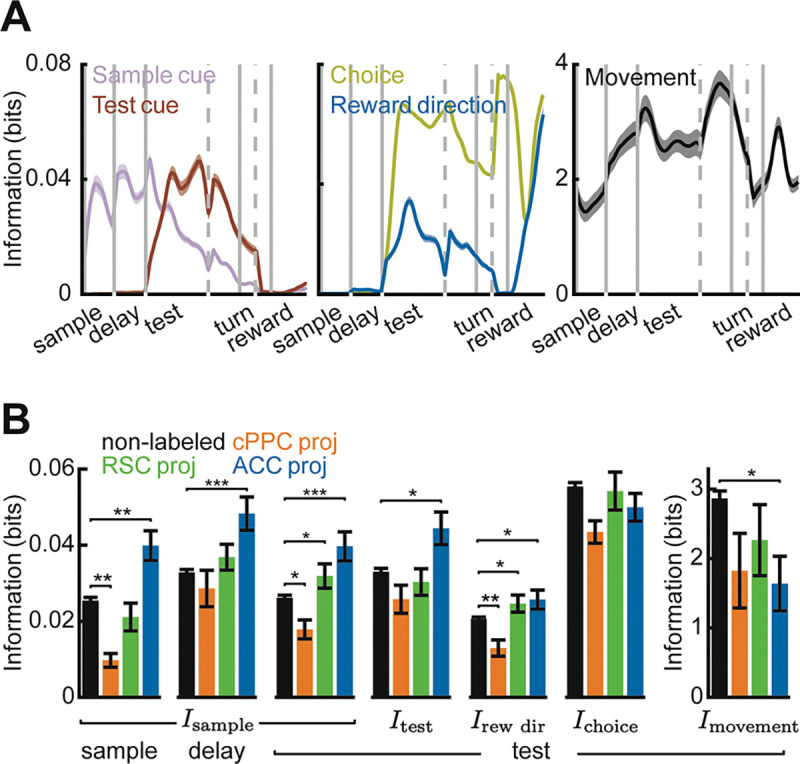
(A) Time-course of different information components in all PPC neurons. Shading indicates mean ± SEM. (B) Average single-neuron information in different populations about different task variables during the first two seconds after sample cue onset, delay onset, or test cue onset (non-labeled cells, cPPC proj: cells, RSC proj: cells, ACC proj: cells). Error bars indicate mean ± SEM across cells. * indicates , ** indicates , and *** indicates , t-test with Holm-Bonferroni correction for statistical multiple comparisons.
To determine if different aspects of task and movement information are transmitted to distinct targets, we compared neurons with different identified projections and the unlabeled cells with unidentified projections. Information for the sensory-related task variables – sample cue, test cue, and their xor combination – was enriched in ACC-projecting neurons and lowest in contralateral PPC-projecting cells (Figure 3B). Thus, PPC preferentially transmits sensory information to ACC. In contrast to sample cue and test cue information, information about the choice and movements was similar across the projection types, indicating that this information is more uniformly transmitted (Figure 3B). However, all three projection types had lower information about the movements of the mouse than the unlabeled cells, suggesting that the movement information is enriched in neurons projecting to areas other than those studied here or in interneurons (Figure 3B, right). In addition, cells projecting to contralateral PPC often had less information about each variable than the unlabeled cells, indicating that across-hemisphere communication may be less critical for encoding specific task and movement events. On the other hand, RSC-projecting neurons carried the information typical of the PPC population, as shown by similar levels of information to the unlabeled neurons. Thus, neurons projecting to different target areas differ in their encoding, revealing a specialized routing of signals from the PPC to its targets. However, each projection class contains a significant level of information about each variable, showing that PPC also broadcasts its information widely.
Enriched information-enhancing pairwise interactions in neurons projecting to the same target
Beyond single-neuron coding, the structure of correlated activity patterns in populations of neurons can impact the transmission and reading out of information7,37. We used the NPvC model to calculate pairwise noise correlations7,37, defined as the correlations in activity for a pair of neurons for a fixed trial type (Supplemental Information, Figure 4A). We focused on the first two seconds after the test cue onset. Remarkably, noise correlations were significantly larger in pairs of neurons projecting to the same target than in unlabeled neurons with unidentified projection patterns (Figure 4B left; Figure S4A), suggesting that correlations aid transmission of information between areas. For all groups of neurons, noise correlations were higher on correct trials than incorrect trials, consistent with the possibility that correlations aid the transmission and reading out of information to guide behavior24 (Figure 4B; Figure S4A). We also considered that behavioral variability within a given trial type, such as differences in running velocities, could contribute to trial-to-trial variability and thus potentially to noise correlations. After conditioning on movement variability using the single-neuron NPvC models, noise correlations were lower, confirming that movement variability contributed to traditional noise correlation measures (Figure 4B right, Figure S4A). However, even in this case, noise correlations were higher in neurons projecting to the same target than in pairs of unlabeled neurons and higher in correct trials (Figure 4B right, Figure S4A).
Figure 4. Pairwise interactions between pairs of non-labeled neurons and pairs of neurons projecting to the same target.

(A) Schematic of the models to compute pairwise joint probability density functions and conditional joint probability density functions of two neurons with correlated activities as a function of time . A vector of movement variables with components is represented. Using single neuron NPvC model outputs, we build different types of pairwise correlation models with and without conditioning over the movement variables. The joint pairwise model is then used to estimate noise correlations or interaction information. (B) Left: Noise correlations computed for pairs of non-labeled neurons and pairs of neurons projecting to the same area for correct and incorrect trials. Right: Same except for noise correlations conditioned on movement variables. (C) Similar to panel (B) but for interaction information. (D) Average single-neuron choice information in different populations during the first two seconds after the test onset for correct and incorrect trials. (E) Histogram of interaction information divided into pairs of information-enhancing (red), information-limiting (blue), and independent pairs (green). In panels (B-D), error bars indicate mean ± SEM across all pairs of neurons. * indicates , ** indicates , and *** indicates , t-test with Holm-Bonferroni correction for statistical multiple comparisons.
Depending on well characterized relationships between the structure of signal and noise correlations, noise correlations can either limit or enhance the information in neural populations7,37. To quantify the effect of noise correlations on information, for each pair of neurons, we decomposed the mutual information between the pair’s activity and a task variable into independent information, defined as the information that the pair would carry if their noise correlations were absent, and interaction information, defined as the difference between the actual information carried by the pair (which includes the effect of noise correlations) and the independent information (Figure 4A). The interaction information thus quantifies how much a neuron pair’s noise correlations increase (information-enhancing) or decrease (information-limiting) information about a task variable. We focused on choice information because it is relevant for guiding behavioral actions and in PPC is larger than sample cue and test cue information.
The average value of interaction information across pairs of neurons was positive, and thus noise correlations were on average information-enhancing (Figure 4C). Remarkably, interaction information on correct trials was larger in pairs of neurons projecting to the same area compared to pairs of unlabeled cells (Figure 4C). Furthermore, interaction information was higher on correct trials than on incorrect trials. For pairs of neurons projecting to the same target, interaction information even dropped close to zero on incorrect trials (Figure 4C). In contrast, in single neurons, the choice information was on average similar in value between correct and incorrect trials (Figure 4D), suggesting a specific role of neuron-to-neuron interactions for generating correct behavioral choices. These results indicate that the pairwise interactions differ in populations projecting to the same target relative to surrounding neurons, that these interactions enhance the information that is transmitted, and that they may be beneficial for accurate decisions.
Interestingly, there was a wide range of interaction information values across pairs of neurons, with extended and almost symmetric positive and negative tails (Figure 4E). We identified pairs of neurons with information-enhancing (significantly positive), information-limiting (significantly negative), and independent (not significantly different from zero) interaction information. Most pairs (~90%) were classified as information-enhancing or information-limiting (Figure S4E). Confirming previous studies37–39, the most important determinant of whether a pair had information-enhancing or information-limiting interaction information was the sign of noise correlations relative to the sign of signal correlations (i.e., the similarity of choice selectivity of the two neurons forming a pair). Pairs with the same sign for signal and noise correlations had information-limiting interactions, whereas pairs with opposite signs for these correlations had information-enhancing interactions (Figures S4H,I). Thus, the PPC population has a rich distribution of information-enhancing and information-limiting pairs.
We also computed the interaction information for individual projection targets and about the sample cue and test cue (Figures S4B,D). RSC-projecting pairs had similar interaction information to unlabeled pairs, consistent with RSC-projecting neurons being most similar to the unlabeled population. For test cue information, we observed similar but weaker results to those reported above for choice. For sample cue information, we did not find differences in interaction information between cells projecting to the same target and unlabeled pairs. Thus, there exists possible specificity of interactions between these neurons with respect to different task variables and projection pathways.
The network structure of pairwise interactions
Two networks that have the same set of values of information-limiting and information-enhancing interactions can differ in how these interactions are organized within the network (Figures 5A,B). For example, the same set of interaction pairs can be distributed either randomly within a group of neurons (Figure 5A, top) or structured as clusters containing enriched information-enhancing or information-limiting interactions (Figure 5A, middle and bottom).
Figure 5. The presence of network structure of interaction information in populations projecting to the same target.

(A) Schematics of a random network (top), a network with clustered interactions (middle), and a network with modular structure (bottom). (B) Sketch of how networks with the identical probability of information-enhancing and information-limiting interactions can be organized randomly or in clusters of information-enhancing or information-limiting pairs. Red and (+) indicates information-enhancing pairs. Blue and (−) indicates information-limiting pairs. (C) Relative triplet probability with respect to a random network for non-labeled and same-target populations during correct (left) and incorrect (right) trials. The random network has the same distribution of pairwise interactions, except shuffled between neurons. (D) Global cluster coefficient of information-enhancing (IE) and information-limiting (IL) sub-networks relative to a random network. (E) Schematic of a two-pool network model. (F) Schematic of the space of two-pool networks is quantified in terms of the probability of information-enhancing pairs in pool 1 (x-axis) and pool 2 (y-axis) minus the probability of these pairs in a random network. Red indicates information-enhancing pools, and blue indicates information-limiting pools. (G) Schematic of some examples of symmetric and asymmetric networks corresponding to different points in the two-pool network space along the diagonal (red dashed line) or antidiagonal (blue dashed line) axes. (H) Left: The probabilities of different triplets computed for different two-pool networks minus the triplet probabilities in a random network, computed analytically as derived in Supplemental Information: Analytical calculation of triplet probabilities in the two-pool model of network structure for two-pool networks. Right: The triplet probabilities for three example model networks sampled from the space of two-pool networks. (I) At each point in the 2D space of two-pool networks, comparison of the triplet probabilities for the model network and the empirical data. The similarity index ranges from 1 for similar networks to 0 for completely different networks. Yellow circles correspond to networks that are more similar to data for non-labeled (left) and same-target projection networks (right). The four dashed contours correspond to two-pool networks with similar value of each of the four triplet probabilities to the one obtained from data (from Figure 5C for correct trials). (J) Using pools of neurons defined based on their choice selectivity to left or right choices, the average interaction information within the pool and between the pools, relative to a random network. Pink indicates same-target projections. Black indicates non-labeled neurons. (K) Similar to (J) but for the probability of information-enhancing pairs within or between pools, relative to a random network. Error bars indicate mean ± SEM estimated using bootstrapping over all triplets. *** indicates , t-test with Holm-Bonferroni correction for statistical multiple comparisons.
Graph-theoretic measures can be used to identify structured arrangements of pairwise links in a network. The simplest measures are defined based on the frequency of interaction triplets, which are the simplest motifs in a graph beyond pairs40,41. For example, a network with information-limiting clusters will have a larger number of ‘−,−,−’ triplets compared to a random network, and a network with information-enhancing clusters will have more ‘+,+,+’ triplets compared to a random network (Figures 5A,B), where ‘−’ and ‘+’ correspond to information-limiting and information-enhancing pairwise interaction links, respectively. For interactions for choice information, we identified the network structure by computing the difference in the probabilities of ‘−,−,−’, ‘−,−,+’, ‘−,+,+’, and ‘+,+,+’ triplets between our data and an unstructured network obtained by randomly shuffling the position of pairwise interactions within the network, without changing the set of values of interactions within the network. In the unlabeled population, triplet probabilities were like those in a random network, indicating that the pairwise interactions are not structured (Figure 5C). However, in populations of neurons projecting to the same target, there was an enrichment of ‘+,+,+’ and ‘−,−,+’ triplets and a relative lack of ‘−,−,−’ and ‘−,+,+’ triplets compared to a random network. Notably, this structure was present only on correct trials and was absent when mice made incorrect choices (Figure 5C). The network structure was present in ACC-, RSC-, and contralateral PPC-projecting populations for choice information but was less apparent for sample cue and test cue information (Figure S5A,B).
We next used a graph global clustering coefficient40,41 to measure information-limiting or information-enhancing clusters. This coefficient measures the ratio between the number of specific types of closed triplets and the number of all triplets, normalized to the same quantity computed from shuffled networks. It thus measures the excess of closed triplets in real data compared to the shuffled network. In populations of neurons on correct trials, the clustering coefficient obtained from data was larger compared to a shuffled network for information-enhancing interactions, meaning that these interactions were clustered together. In contrast, for information-limiting interactions, the clustering coefficient was smaller than for a shuffled network, indicating that they were preferentially set apart (Figure 5D). This clustering was mostly absent in unlabeled neurons and when mice made incorrect choices (Figure 5D). These results thus reveal the presence of pairwise interaction clusters in the network of neurons projecting to the same target.
To exemplify how the network’s topology relates to the triplet distributions, we considered a simple two-pool network model in which the network structure can be varied parametrically, while keeping the overall set of values for information-enhancing and information-limiting interactions constant (Figure 5E). Each pool was parameterized by the difference in probability of information-enhancing pairwise interactions within the pool relative to a random network. Thus, the range of possible network models resides in a two-dimensional space consisting of the enrichment of information-enhancing interactions in pool 1 along one axis and in pool 2 along the second axis (Figure 5F). In this parameterization, the diagonal corresponds to symmetric networks, in which both pools have more information-enhancing or more information-limiting interactions than expected in a random network. The antidiagonal corresponds to asymmetric networks, with one pool having more information-enhancing interactions and the other having more information-limiting interactions. Networks near the origin are similar to a random network.
For every point in the two-dimensional space of network models, we analytically computed the triplet probabilities compared to a random network (Figure 5H, left). We then used these model predictions of triplet probabilities to map the triplet probabilities estimated in our empirical data back into the parametric model (Figure 5I). Populations of cells projecting to the same target mapped to a symmetric network with both pools having enriched within-pool information-enhancing interactions and elevated across-pool information-limiting interactions (Figure 5I, right). In contrast, the population of unlabeled neurons mapped to a point close to the origin, corresponding to a randomly structured network (Figure 5I, left).
What factors define the neurons that participate in the pools with enriched within-pool information-enhancing interactions and elevated across-pool information-limiting interactions? One commonly studied factor is the selectivity of neurons. We divided neurons into two pools based on their choice selectivity (i.e., left vs. right choice selectivity) and compared these pools to a network with shuffled pairwise interactions. For unlabeled neurons, the interaction information and proportion of information-enhancing interactions were similar to the random network both within pools of neurons with similar choice preferences and across pools with different preferences (Figures 5J,K). In contrast, for neurons with the same projection target, pools of cells with the same choice preference had higher interaction information and a larger proportion of information-enhancing interactions than the random network (Figures 5J,K). Further, in these same-target projection populations, cell pairs with opposite choice preferences had lower interaction information and an enrichment of information-limiting interactions. This structure was strong on correct trials and largely absent when mice made incorrect choices. Thus, the network structure we described above was present in pools of neurons defined by choice preference.
Together, these results reveal rich structure in the pairwise interaction information that is approximated by a network of symmetric pools with enriched within-pool information-enhancing interactions and across-pool information-limiting interactions. This structure can be in part conceptualized in terms of organization according to the neuron’s choice selectivity. Strikingly, this structure was only present in neurons projecting to the same target, not in neighboring unlabeled neurons, and only when mice made correct choices, suggesting this structure could be significant for the propagation of information to downstream targets in a manner that is important for accurate behavior.
The contribution of the network structure of pairwise interactions to population information
What are the consequences of this network-level structure of pairwise interactions on the information encoded in a neural population? To address this question quantitatively, we analytically expanded the information encoded by the population about a given task variable as a sum of contributions of interaction graph motifs. Under the assumption that single-pair interaction information values are small compared to single-neuron information (as is the case in our empirical PPC data; compare Figures 4C,D), the population information can be approximated as a sum of, in order of increasing complexity (Figure 6B), contributions of nodes (single neuron information), links (pairwise interaction information), and triplets (triplet-wise arrangements of pairwise interaction information). In Figures 6B–D, we illustrate this expansion for the simple case of a symmetric network, which describes well our empirical data. However, for calculating information, we used a complete and general expansion of population information that is valid also for non-symmetric networks (Supplementary Methods and Figure S7D).
Figure 6. The contribution of network structure of interaction information to the population information.

(A) Schematic of how the population information can be decomposed into three components: independent information, unstructured interaction information, and structured interaction information. (B) The population information can be expanded as a sum of contributions from network motifs with increasing complexity. For a symmetric network, the dominant contributions are from single neurons, interaction pairs, and interaction triplets. (C) In symmetric networks, triplets contribute to structured interaction information with a positive or negative sign if they have an even or odd number of information-limiting interactions, respectively. (D) Structured interaction information in the space of symmetric two-pool networks. The structured interaction information can be information-enhancing or information-limiting depending on whether the pools have enriched information-enhancing or information-limiting pairs. Pink and black points correspond to the networks of same-target projection and non-labeled neurons, respectively. (E) Independent, unstructured interaction, and structured interaction information for non-labeled (black) and same-target projection (pink) neurons during correct and incorrect trials for increasing population size. Shading indicates mean ± SEM estimated from bootstrapping over triplets. *** indicates , t-test with Holm-Bonferroni correction for statistical multiple comparisons at population size.
We then used the results of this expansion to break down the total information about the task variable carried by the population into three components (Figure 6A), quantifying how pairwise correlations and its structure shape information encoding in the population. The independent information is the information that would be encoded if the population had the same single-neuron properties but zero pairwise noise correlations 7,38,42,43. The interaction information, which is the difference between the total population information and the independent information, was further broken down into two components. The unstructured interaction information component is the information in a population with the same values of pairwise interactions as the data, but randomly rearranged across neurons by shuffling (thus no network structure), minus the independent information. This component quantifies the contribution of the values of pairwise interactions to the population information. The structured interaction information component is defined as the difference between the total population information of the original network and the population information in an unstructured network (Figure 6A). This component isolates the contribution of the structure of pairwise interactions in the network.
The structured interaction information depends on the triplet-wise arrangements of pairwise interaction information because triplets recapitulate the network-level organization of pairwise interactions. Based on analytic calculations presented in the Supplemental Information, each triplet contributes to the structured interaction information with a sign that depends on the product of the signs of its pairwise interactions (Figure 6C). There is a positive contribution for {‘+,+,+’, ‘−,−,+’} triplets and a negative contribution for {‘−,−,−’, ‘−,+,+’} triplets. The sign of the structured interaction information component therefore depends on the difference in the probability of triplets in the original network relative to a shuffled network lacking structure. The magnitude of the structured interaction information depends on these triplet probabilities as well as the single neuron information and pairwise interaction values contained within the triplets.
To visualize how structured interaction information changes with the topology of the network, we computed the value of the structured interaction information component in the simple two-pool network defined in the previous section, making the additional assumption that the values of single neuron information and the absolute values of interaction information per triplet are homogeneous across the network (Figure 6D). In the case of a symmetric network, networks with enriched information-enhancing pools (compared to a randomly structured network) have structured interaction information that is information-enhancing (Figure 6D). In contrast, symmetric networks with enriched information-limiting pools (compared to a randomly structured network) have negative structured interaction information (Figure 6D).
Then, using the single neuron information, pairwise interactions, and triplet probabilities estimated from our PPC data, we computed the independent, the unstructured interaction, and the structured interaction components of the population information for choice (for a symmetric network (Figure 6E) and for a general non-symmetric network (Figure S7D)). The independent information was the largest component and was similar between neurons projecting to the same target and unlabeled populations (Figure 6E, left). The unstructured and structured interaction information contributed less to population information, as expected from the findings reported above that pairwise interaction information values were smaller than single-neuron information values (c.f., Figures 4C,D). Strikingly, the contributions of both structured and unstructured interaction information were markedly larger for neurons projecting to the same target than for unlabeled neurons (Figure 6E, middle, right). The larger unstructured interaction information for populations projecting to the same target is a consequence of their higher pairwise interaction values. The higher structured interaction information for populations projecting to the same target is instead a consequence of the network structure that they exhibit (Figure S7E). The structured interaction information contributed close to zero in the unlabeled population, consistent with the lack of network structure in the unlabeled population. The structured interaction information in the cells projecting to the same target was positive and information-enhancing, consistent with this population having a symmetric network structure with enriched within-pool information-enhancing interactions and across-pool information-limiting interactions compared to a randomly structured network.
Importantly, both mathematical calculations (see Supplementary Information) and numerical evaluations (Figure 6E) show that the contribution of structured interaction information scales faster with increasing population size than the two other components, indicating that this structured interaction information could be an important factor in populations of hundreds of neurons, as are likely involved in biological computations (Figure 6E). In addition, the structured interaction information was mostly absent on incorrect trials, whereas independent information was largely unchanged, suggesting that the structure of network interactions may play a role in guiding accurate behavior.
We found similar trends for network structure for choice information for the populations of neurons projecting to contralateral PPC, RSC, and ACC (Figure S6C). Consistent with the differences in the triplet probabilities for sample cue and test cue information with respect to the choice information (Figure S5A), we found that the network information is either information-enhancing or information-limiting when computed for sample cue or test cue information (Figure S6B), suggesting specificity of network structure with respect to the information content.
Together, these results reveal a rich structure in the pairwise interactions within a population, providing significant insight into the population code compared to models that only consider the mean values of pairwise correlations. Strikingly, this network structure enhanced information levels and was only present in cells projecting to the same target and when mice made correct choices. Thus, populations of PPC cells projecting to the same target are organized in a specialized manner to enhance the propagation of information to downstream targets, potentially impacting accurate decision-making.
Discussion
The understanding of how the properties of population codes emerge from the interactions among neurons has been built on studies of information coding in populations of all neurons recorded from a given location, without identifying those that may be read out as a group. Because populations of nearby cortical neurons project to a wide diversity of targets, these previous studies have probably mixed neurons that are read out by different downstream networks. Instead, by studying population codes from the perspective of neurons that project to the same target area, we discovered properties that are unique to these populations and absent when considering all recorded neurons in PPC, including stronger pairwise correlations and a structured manner in how pairwise correlations are organized within the population. Thus, neurons comprising an output pathway in PPC form specialized population codes.
A first specialized feature of codes of populations projecting to the same target area is an elevated strength of pairwise correlations, with respect to neighboring neurons. Because correlated activity in PPC and other areas supports reliable propagation of information23,24,44 and because correlations are stronger in correct trials, elevated correlation levels may be present to support behavior by enhancing the efficacy of transmission of information to downstream areas. A second specialized feature of codes of populations projecting to the same target area is the presence of a network-level structure of pairwise interactions that enhances the population’s information about the mouse’s choice, even though it is made up of a diverse mix of information-enhancing and information-limiting pairwise interactions. While the information provided by the network structure is small relative to single neuron information values in small populations of neurons, we estimate that it grows rapidly with population size and provides a substantial fraction of the information carried by the whole population projecting to a specific area. In addition, the network-level structure is present only when mice make correct choices during the task and is absent when mice make incorrect choices, suggesting that the information carried by this structure is key to correct behavior. Whereas some previous work has suggested that populations must trade off the disadvantage of correlations for limiting information levels with the benefit for robust signal propagation7,24,26,44–47, the output pathways we studied might use this specialized interaction structure in population codes to simulatenously optimize multiple goals, including information encoding and information transmission. It will be of interest to understand how these specialized features of population codes arise from circuit connectivity. It is possible that structured local connections between cells in the same output pathway play a critical role48.
Previous work has focused on how pairwise and higher-order correlations shape the information encoded in a population, including establishing principles for how signal and noise correlations combine to give rise to pairwise information-limiting or information-enhancing interactions7,37,49–53. However, these effects have mainly been studied without taking into account how these interactions are arranged as a network. Networks with identical sets of values of pairwise interactions can have these interactions arranged in a random manner or with various types of structures. Recent work has moved in this direction finding that network-level structure exists, with redundant and synergistic interactions tending to form separate hubs in visual cortex8. Other work has investigated the structure of functional connectivity with graph theory or network science and revealed how principles of network organization (e.g., rich-club structure) relate to aspects of network dynamics, such as speed or robustness54. In many cases, it remains unstudied if and how these principles of network organization enhance or limit the encoding of information, especially in the context of decision-making tasks. Yet other work has begun to develop methods to look at the communication between brain areas based on larger scale population activity2,55,56. However, connections between the population geometries revealed with these approaches, the structure of pairwise correlations, and information encoding remain to be investigated. Our results build on these previous lines of research by directly identifying neurons comprising an output pathway and demonstrating how the existence of structured task-relevant information interactions in these populations impacts information encoding. In addition, we established a general framework to link network-level structures to its information-enhancing or information-limiting effect for population codes. It will be of interest to apply this approach to other communication pathways and types of tasks and behavioral information. Here, we found that the network-level structure was present across projection pathways for choice information but was less strongly apparent for other types of information.
Our analysis was facilitated by the development of NPvC models that can estimate the relationships between variables in a large multivariate setting even if the form of these relationships is unknown or complex (Figure S4G). Because these models described the neural activity better than simpler models such as GLMs, we could more effectively discount potential covariations between task and movement variables in the estimates of population information. This facilitates the removal of the covariations due to the common tuning to movement variables of many neurons18,19,30,57, which may induce large covariation-based redundancies masking the structure of the underlying information-enhancing and information-limiting interactions. Further development and application of copula-based methods to neuroscience will aid the analysis of relationships in high dimensional behavioral and neural data, including the structure and information content of neural correlations in larger scale neural recordings58.
PPC broadcasts information about the task variables to all the targets we studied here. While there was large overlap in the encoding of ACC-, RSC-, and contralateral PPC-projecting neurons, we observed some specificity in the types of information transmitted in these pathways. Most notably, sensory-related information was strongest in the ACC-projecting neurons, consistent with streamlined sensory and motor communication pathways between parietal and frontal cortical areas59. In contrast, contralateral PPC projections tended to carry less information about the task, implying that cross-hemisphere interactions may serve a role other than computing specific task quantities, such as choice, and instead may be more involved in maintaining consistent activity patterns60. All three intracortical projection pathways had lower information about the movements of the mouse, indicating that cells projecting to other targets, perhaps subcortical areas, might be more related to the biasing of movements. This finding could be consistent with corticostriatal projections from PPC carrying action selection biases61. Collectively, these findings support the notion of specificity in the information flow in cortex62–65. Simultaneously, the presence of information about each task and movement variable in each output pathway fits with many findings of highly distributed representations across cortex and with work that has failed to identify categories of neurons in PPC based on activity profiles18,19,21,29,30,65–67.
Together, our findings demonstrate that specialized network interaction structures in PPC aid the transmission of choice signals to downstream areas, and that these structures are potentially important for guiding accurate behavior. In addition, our results suggest that the organization principles of neural population codes can be better understood in terms of optimizing transmission of encoded information to target projection areas rather than in terms of encoding information locally.
Methods
Mice
All experimental procedures were approved by the Harvard Medical School Institutional Animal Care and Use Committee and were performed in compliance with the Guide for Animal Care and Use of Laboratory Animals. Imaging data were collected from 10 male C57BL/6J mice that were eight weeks old at the initiation of behavior task training (stock no. 000664, Jackson Labs).
Virtual reality system
The virtual reality system has been described previously25. Head-restrained mice ran on an 8-inch diameter spherical treadmill. A PicoP micro-projector was used to back-project the virtual world onto a half-cylindrical screen with a diameter of 24 inches. Forward/backward translation was controlled by treadmill changes in pitch (relative to the mouse’s body), and rotation in the virtual environment (virtual heading direction) was controlled by the treadmill roll (relative to the mouse’s body). Movements of the treadmill were detected by an optical sensor positioned beneath the air-supported treadmill. Mazes were constructed using VirMEn in MATLAB68.
Behavioral training
Prior to behavioral training, surgery was performed in 8-week-old mice to attach a titanium headplate to the skull using dental cement. At least one day after implantation, mice began a water schedule, receiving at least 1 ml of water per day. Body weights were monitored daily to ensure they were greater than 80% of the original weight. Mice were trained to perform the delayed match-to-sample task using a series of progressively complex mazes. Mice were rewarded with 4 μl of water on correct trials. First, naive mice were trained to run down a straight virtual corridor of increasing length for water rewards. In the second stage, mice learned to run in a T-shaped maze, into either a left or right choice arm. The correct choice arm was signaled by the presence of a tall tower at the choice arm. After the mouse was able to run straight on the ball and make turns, we trained mice on stage 3, where we began to familiarize the mice with running into the choice arm that matches the color presented in the maze stem (sample cue). The walls of the stem were either black or white (sample cue; randomly selected from trial to trial). The left and right choice T-arms were black and white, respectively, or vice versa (test cue). At this stage of training, the correct choice arm was signaled both by a tall tower in the correct arm and by the T-arm that matched the color of the sample cue. Note that in this stage, the mouse can still perform accurately even if it ignores the sample and test cues, as it can just run to the choice arm that has the tower. In the fourth stage, the maze was the same, except that we added a tower to the unrewarded choice arm as well. In this stage, the mouse cannot simply run to whichever arm has a tower (since both arms have towers) and must run into the arm that matches the color of the sample cue. In stage four, the maze was exactly like the previous one, except the choice arms and towers (test cue) appeared grey as the mouse ran down the maze. The colors of the choice arms and towers (test cue) were not revealed until the mouse reached 3/4 of the way down the stem. When the black and white choice arms were revealed, the mouse can begin to plan and execute a turn left or right. In the final stage, we begin training towards the final implementation of the delayed match-to-sample task. We introduced a delay segment by making the walls of the T-stem grey at the end of the stem and gradually increased the length of the stem that is grey (delay segment). The mouse received its first trials of the delayed match-to-sample task when at least the entire last 1/4 of the stem walls were grey. In such trials, when the mouse’s position reaches 3/4 of the way down the stem, there was a short moment in which both the stem walls and the choice arms were grey. At this point, the mouse must rely on its memory of the initial sample cue walls to make the correct turn. We made this grey segment longer and longer until the mouse performed with over 85% accuracy for a delay averaging at least two seconds in duration. The entire training program was completed in 12–18 weeks.
Surgery
When mice reliably performed the delayed match-to-sample task, the cranial window implant surgery was performed. Mice were given free access to water for two days prior to surgery. During the surgery, mice were anesthetized with 1.5% isoflurane and the headplate was removed. Craniotomies were performed over PPC centered at 2 mm posterior and 1.75 mm lateral to bregma. GCaMP6 was injected at 3 locations spaced 200 μm apart at the center of the PPC. A micromanipulator (Sutter, MP285) moved a glass pipette to approximately 250 μm below the dura, and a volume of approximately 50 nL was pressure-injected over 5–10 minutes. Dental cemented sealed a glass coverslip on the craniotomy, and a new head plate was implanted, along with a ring, to interface with a black rubber objective collar to block light from the VR system during imaging. Craniotomies were also performed over the contralateral PPC (2 mm posterior and 1.75 mm lateral to bregma), anterior cingulate cortex (1.34 mm anterior and 0.38 mm lateral to bregma, and 1.3 mm ventral to the surface of the dura). Over 200 nL of retrograde tracer (CTB-Alexa647, CTB-Alexa405, or red retrobeads) was injected at each site. The retrograde tracer injection into RSC was made through the craniotomy for PPC imaging, targeting the most medial portion of the craniotomy (~0.5 mm lateral from the midline). Craniotomies for the retrograde tracers were sealed with KwikSil (World Precision Instruments). Mice recovered for 2–3 days after surgery before resuming the water schedule. Imaging was performed nearly daily in each mouse, starting 2 weeks after surgery, and continued for 1–2 weeks.
Obtaining anatomical stacks
Anatomical stacks of cells double-labeled with GCaMP and retrograde tracers were acquired using a two-photon microscope taken every 2 μm from the surface of the dura to about 300 μm below the surface. For images of cells double-labeled with GCaMP and CTB-Alexa647, we used a dichroic mirror (562 long pass, Semrock) and bandpass filters (525/50 and 675/67 nm, Semrock) and delivered the excitation light at 820 nm to visualize both GCaMP and the Alexa fluorophore simultaneously. We also took images of GCaMP and CTB-Alexa405 using a dichroic mirror (484 long pass) and bandpass filters (525/50 and 435/40) and delivered excitation light at 800 nm. Finally, we took images of GCaMP and red retrobeads with dichroic mirror (562 long pass) and bandpass filters (525/50 and 609/57) and delivered excitation light at 820 nm. These anatomical stacks allowed us to identify cells later visually as either double-labeled with GCaMP and retrograde tracer or GCaMP-expressing and unlabeled with retrograde tracer. We then matched these GCaMP-expressing neurons from the anatomical stacks with the same GCaMP-expressing neurons during functional imaging, which was performed at 920 nm and during behavior. In some sessions, we took z-stacks immediately before functional imaging to ensure some labeled cells were present in a field of view.
GCaMP imaging during behavior
For functional imaging, 5 mice were imaged using a Sutter MOM at 15.6 Hz at 256 × 64-pixel resolution (~250 × 100 um) through a 40x magnification water immersion lens (Olympus, NA 0.8). Five other mice were imaged using a custom-built two-photon microscope with a resonant scanning mirror (at 30 Hz frame rate) with a 16x objective. ScanImage was used to control the microscope. Imaging sessions lasted 45–60 minutes. Each session was imaged over multiple 10-minute acquisitions separated by 1 minute, allowing any amount of GCaMP bleaching to recover. The imaging frame clock and an iteration counter in VirMEn were recorded to synchronize imaging and behavioral data.
Data processing
Custom-written MATLAB software was designed for motion correction, definition of putative cell bodies, and extraction of fluorescence traces (dF/F). Fluorescence traces were deconvolved to estimate the relative spike rate in each imaging frame and all analyses were performed on the estimated relative spike rate to reduce effects of GCaMP signal decay kinetics.
To estimate the neural activity of individual cells from the calcium imaging data, we processed the data by the following steps. (1) Motion correction: Motion artifacts in imaging data were corrected in each imaging frame. First, “line-shift correction” was performed to align for line-by-line alternating offsets in images due to bidirectional scanning. Then, “sample movement correction” was performed to remove between-frame rigid movement artifacts by FFT-based 2d cross-correlation 69 and within-frame non-rigid movement artefacts by Lucas-Kanade method 70. (2) Cell selection: The spatial footprint of a putative cell was identified based on the correlation of fluorescent time series between nearby pixels. The correlation of fluorescence time series was calculated for each pair of pixels within a ~60 × 60 μm square neighborhood. Then putative cells were identified by applying a continuous-valued, eigenvector-based approximation of the normalized cuts objective to the correlation matrix, followed by discrete segmentation with k-means clustering, which generated binary masks for all putative cells. (3) dF/F calculation: The magnitude of calcium transients was estimated by subtracting the background fluorescence from the raw fluorescence of a putative cell. For each putative cell, the background fluorescence of local neuropil was estimated by the average fluorescence of pixels that did not contain putative cells. Then neuropil fluorescence time series was scaled to fit the raw fluorescence of a putative cell by iteratively reweighted least-squares (robustfit.m in MATLAB) and was subtracted from the raw fluorescence to yield neuropil-subtracted fluorescence (Fsub). Then, dF/F was calculated as , where was a linear fit of using iteratively reweighted least-squares (robustfit.m in MATLAB). The codes used in steps (1–3) are available online: (https://github.com/HarveyLab/Acquisition2P_class.git).
(4) Deconvolution: The timing of spike events that led to calcium transients was estimated by deconvolution of fluorescent transients. dF/F was deconvolved by OASIS AR1 71, which models the fluorescence of each calcium transient as a spike increase followed by an exponential decay, whose decay constant was fitted to each cell. The deconvolved fluorescence resulted in spikes that were sparse in time and varied in magnitude. The deconvolved fluorescence was used as neural activity for the majority of the analyses.
Non-parametric vine copulas (NPvC) models of single neuron activity
To quantify the information carried by a neuron’s activity about task variables, while discounting possible contributions from movement variables, we built a multivariate probabilistic model of the activity of each neuron, time, behavioral variables (running velocity and acceleration), and task variables (schematized in Figure 2C). We built this model using non-parametric vine copulas (NPvC). We chose vine copulas because they allow constructing arbitrarily complex multivariate relationships (including relationships between non-neural variables, e.g. relationships between trial types and behavioral variables) by combining bivariate relationships, which can be sampled accurately and robustly from finite number of trials regardless of the details of the marginal distributions. We chose non-parametric estimators because the form of these relationships is not known a priori and we wanted to avoid biases originating from inaccurate assumptions. Here, we describe the details of the computation of our non-parametric vine-copula model, specifically for computing the probability density function of neural population activity given behavioral and task variables at each time point in the trial (Figure 2D) and for computing its goodness of fit (Figure 2E).
We used vine copulas to estimate the conditional joint probability density function for a set of variables , which in our case consists of the activity of a neuron , time and the 5-dimensional vector of the five behavioral variables that we measured (virtual heading direction, lateral and forward running velocities, and lateral and forward accelerations), for each trial type . Each trial type is defined by the sample cue, the test cue, and trial outcome (correct or incorrect). Thus, there are four trial types for trials with correct choices and four trial types for incorrect trials. Using the copula decomposition, the probability density function for each trial type is represented as a product of the single variable marginal probability density functions , and the copula , which captures the dependencies between all the variables, as follows:
| (M1) |
We used a kernel density estimator 72 to compute the single-variable marginal probability densities and a non-parametric c-vine vine copula to estimate the copula, representing the correlation structure between variables. We used a c-vine graphical model with neuron activity as the central variable in the model. The probability density function of a c-vine can be expressed as the product of a sequence of non-parametric bivariate copulas 31,73 (Supplemental Information: Vine copula modelling of neural responses). We used similar order for the variables in the c-vine graphical model as introduced above. Furthermore, we simplified the vine copula structure by considering the decomposition of the copula as a product of a time-dependent and a time-independent component meaning that we considered that the tuning of neurons to movement variables is time-independent. The sequence of bivariate copulas shaping the vine-copula were then fitted to the data using a sequential kernel-based local likelihood process (Supplemental Information: Nonparametric pairwise copula estimation)34. For each of the bivariate copulas, the kernel bandwidth was fitted so as to maximize the local likelihood obtained in a 5-fold cross-validation method 34. Using the estimated bandwidths for each copula in the vine sequence, we computed the multivariate copula density function of data points using a 5-fold cross-validation process. We first used the training set to estimate the copula density on a 50 by 50 grid (Supplemental Information: Nonparametric pairwise copula estimation) and then used the copula estimated on the grid point to interpolate the copula density on the test set. A similar procedure was followed to estimate cross-validated single variable marginal density functions. The conditional probability of neural responses in each trial condition and for each value of behavioral variables is computed using where to compute the density function , we marginalized by integrating over the neuron response
| (M2) |
In Eq M2, we approximated the integral as a sum over a set of points ranging linearly between the minimum and maximum value of the neural response within the session and . By computing the density function by marginalization of , instead of fitting a new vine model between variables, any difference between these two density functions is only related to the dependency of the neural activity to other variables and not to a difference between how dependencies between variables are being quantified in the two models because of fitting differences.
For each time point, we computed a copula fit of the activity of each neuron (indicated as NPvC fit in Figure 2D) as a point with largest log likelihood given the considered trial type and the values of behavioral variables at the considered time point:
| (M3) |
Generalized Linear Models (GLMs) of single neuron activity
We also fit a GLM model to compare it with the copula. We used a GLM with Poisson noise, a logarithmic link function, and an elastic-net regularization23,26,35. We used task variables defining the trial type consisting of sample cue, test cue, choice, and all their interactions (each binary task variable was coded as −1 or +1) together with the same behavioral variables we used in copula modelling as the predictors. Time-dependency during the task for single neurons was expanded using a raised cosine basis 26 as follows:
| (M4) |
For task variables, the cosine basis function has a width of 1 s, and the value at the center peak was either positive or negative depending on the identity of each task variable. The center peaks were spaced with a 0.5 s interval to tile the epoch with a half-width overlap. For selectivity to movements of the mouse, we first z-scored each movement variable as and used similar cosine basis as follows:
| (M5) |
We considered 13 center peaks ranging from −3 to 3 with spacing of 0.5 for the cosine basis of movement variables.
Computation of neural data fitting performance of NPvC and GLMs
The performance of both the NPvC and the GLM in fitting single-trial single-neuron activity was evaluated by computing the fraction of the deviance explained (FDE) on the test data, defined as follows 74:
| (M6) |
where , and are the likelihoods of observing the test data for the considered model (copula or GLM), the null model, or saturated model, respectively and are always computed for all the time points in all trials in a cross-validated fashion. For the GLM, the null model is a model that does not have any predictors, and its prediction of activity at any time point is the time-averaged rate of the neuron. For the copula null model, we defined a model of neural response without including any of the predictors in the trial, which quantifies how much of the neural activity can be explained without knowing the time and movement variables used in the vine copula model. The likelihood is then computed using the marginal distribution of neural activity . The saturated model is the generative model in which the prediction exactly matches the observed activity at each time point in the test data. For the GLM, these values were computed using the analytical form of the GLM output at each time point using the logarithmic link function. For the copula model, which is nonparametric, the vine-copula model is used to compute the likelihood for each neural activity as the model likelihood where is the real single trial neural activity at time t from data. To compute the saturated likelihood, we considered the fact that the model prediction is derived from Eq. M3 and the saturated likelihood was considered to be the peak likelihood obtained where is the set of grid points on the neural activity described before ranging from the minimum to maximum possible neural activity of each neuron. Each of the likelihood values on the data were computed using a 5-fold cross-validation. The density function is estimated over a grid using the training set, and the grid is used to compute the density function over the test set (Supplementary Method 2). We considered five different task epochs and fitted the model to each of them. The periods were from 0.5 s before to 2 s after the sample cue onset, delay onset, test cue onset, start of the turn, and reward onset. We used only sessions that had at least 5 trials of each of the 8 trial types.
Estimation of Mutual information for single neurons
We used probabilities estimated from the vine-copula approach, explained in the previous section, to estimate single neuron mutual information values (presented in Figure 3). To compute the mutual information between a group of variables (including neural activity and/or behavioral variables) and a task variable, we used a decoding approach and then computed information in the confusion matrix75–77. A task variable here was a binary variable taking a value of +1 or −1 to indicate one of the two possible values of either sample cue, test cue, reward location, or choice direction. For each task variable, we decoded its value in each trial using the copula model to compute (through Bayes’ rule) the posterior probability of the task variable given the observation in the same trial of a set of variables , which could be the full set . or a subset of it. This posterior probability of can be obtained from the copula model as follows:
| (M7) |
where the sum is over all the trial types (corresponding to the combinations of two sample cues, two test cues, and two trial outcomes (correct or incorrect) and consists of eight possible values when using all trials and four values when using either correct or incorrect trials) which have value for the considered task variable. For example, considering analyses limited to correct or incorrect trials the sum will be over the 4 correct or incorrect trial types. Considering analyses using all the trials the sum will be over all 8 trial types. Considering sample cue correct trials only, the sum in Eq. M6 will be over the two trial types with correct outcome and two sample cues, and so on. is the probability of occurrence of trial type across all considered trials. In the above equation, the probability density of the variable given the trial type , is computed using the copula model by using Eq. M1 when or using Eq. M2 when .
We then used the posterior probabilities to decode the most likely task variable given the variables observed in the considered trial:
| (M8) |
The information about the task variable decoded from neural activity was then computed as the mutual information between the real value of the variable and the one decoded from neural activity, as follows:
| (M9) |
where is the confusion matrix, that is the probability that the true value of the task variable is and the value of the decoded one is , and and are the marginal probabilities.
To compute the information between the task variable and the neural activity at a given time point, conditioned over the behavioral variables, we used the following equation for conditional mutual information:
| (M10) |
In the above equation, was computed after decoding using the copula derived from Eq. M1. , was computed after decoding using the copula constricted with Eq. M2 a .
We computed the mutual information between the neural activity and the behavioral variables at time (used in Figure 3A–B) using Shannon’s mutual information formula with probabilities defined by the copula , the marginalized copula , and the probability of each trial type as follows:
| (M11) |
The entropies and were computed by averaging the corresponding NPvC estimated log-likelihoods at the neural activity and movement values sampled from the trial type at each time point.
For the information about the task variables, we chose a computation of information from the decoding matrix, similar to e.g.23, because when computing neural population information about categorical values this computation is robust and has a lower variance and bias than a direct computation from the probabilities. The reason is because the decoding step compresses the dimensionality of the neural responses from which information is computed, especially when considering neuron pair responses and interaction information. This computational robustness was useful because we wanted to use the information values for each neuron pair about task variables at the single neuron and the single pair levels. For the information values about behavioral variables, it was not useful to do the decoding and confusion matrix information computation because the space of the behavioral variables was larger than that of the neuronal activity, and thus we used a direct calculation of information through Shannon formula from the response probabilities. To correct for the limited sampling bias in the information estimation, we computed a shuffled information distribution by repeating the same process after shuffling the label for the trial type (for trial type information Eq. M9) or the neural activity (for the Eq. M10 information) 1000 times and subtracted the mean of the shuffled distribution from the estimated mutual information to correct for the bias78.
Calculation of noise correlations from pairs of neurons
We computed the noise correlations between each pair of neurons (Figures 4, 5, 6) as rank correlations using the estimated cumulative distributive function (CDF) computed with the copula. We first computed the rank of each activity at each time by evaluating its CDF computed through the copula (CDF is a measure of rank percentile79, because it measures the fraction of points with a value lower than the considered one). To compute the noise correlation, we pooled the CDFs computed for the activities in single trials, from the same trial condition, over the first two seconds after the test cue onset and computed the Spearman correlation coefficient. To compute the CDFs at fixed trial type, we first computed the conditioned marginal density functions for each neuron and to compute noise correlations at fixed trial type conditioned on the behavioral variables, we used the NPvC to compute the conditional marginal density functions which allows us to specify the rank specific to the observed value of the behavioral variables at the considered time point for each neuron. To compute the CDFs for each of these density functions, we first computed the CDF over a grid with 200 points on the axis ranging from the minimum to the maximum possible neural activity values by numerical integration of the density function (using the integral definition of CDF). We then used the CDF values on the grid to compute the CDF at each value of neural activity in each trial and time point by interpolation over the grid. Using CDFs and copulas to compute noise correlations has been shown to be robust and accurate in the estimation of noise correlations in neurons80.
We used Spearman correlation coefficients of the neural activity ranks computed from the copula rather than from the real data because the calculation of the ranks conditioned on the behavioral variables could not be performed directly from the data (because the behavioral variables span a continuum that cannot be sampled with a finite number of data points).
Estimation of interaction information and of NPvC models for pairs of neurons
Following previous work81, for any pair of neuron with activity , the interaction information about a task variable for the pair of neurons was defined as the difference between the pairwise information about the task variables carried by the joint observation of the pair of neuron (which reflects both single neuron properties and the effect of interactions between neurons) and the independent information , which reflects only single cell properties and is defined the information for the pair of neurons when they are conditionally independent.
Importantly, in computing interaction information, we also conditioned over the movement variables (as we did for as for single neuron information) in order to isolate the part of the interaction that is related to the task variable selectivity. Conditioning removes the interaction emerging from shared movement selectivity and correlations between the task and movement variables. Thus, interaction information was computed as follows:
| (M12) |
To compute the full and independent information components, we first estimated the pairwise and independent probability density functions and for each trial type respectively. The full probability density function was estimated using the following breakdown of the density function
| (M13) |
The independent probability density function was estimated using a similar breakdown
| (M14) |
The extra component in the full density function, Eq. M13, , is the neuron-pairwise copula term, which represents the interaction between pairs of neurons for the fixed trial condition and conditioned over the movement variables at any time . This term was computed (conceptually similarly to the computation of conditional noise correlation explained above) by building a bivariate copula between the values of conditioned probability functions of the pair of neurons we use the definition of copula as the density function between the cumulative density functions of data, , where denotes the cumulative density function computed from integrating over the density function. To compute this copula, we assumed that the conditional copula density is independent from the value of the movement variables at each time point, i.e., , also note as simplifying assumption. We note, however, that this quantity still depends on the average shared co-tuning of the two neurons to movement variables through the single neuron cumulative density functions. This copula is estimated by pooling the values of conditioned probability functions at each time point for a given trial type.
To compute each of the conditional marginal densities , where indicates the neuron index, we used the single neuron NPvC models we fitted for single neurons and the following identity
| (M15) |
The density functions and were numerically estimated as explained in Section Methods: Probabilistic models of neural activity. All these densities functions were estimated using the same 5-fold cross-validation method explained in Section Methods: Probabilistic models of neural activity.
After computing the density functions of Eqs. M7–M9, we used the same decoding approach as for single neuron information values (see Section Methods: Mutual information estimation) to compute the information values in the right-hand side of Eq. M12, and at any time point. The only difference compared to the single neuron information computation is that to compute the decoded task variable (which is used later to compute the confusion matrix), we used the pairwise density functions (Eqs. M14, M15) instead of single neuron density functions.
We labeled each pair of neurons as information-limiting, independent, or information-enhancing if the mean of the interaction information for the pair in the first two second after the test cue onset was significantly negative, not different from zero, or positive, respectively. We computed the statistical significance of the sign of pairwise interaction information by building a bootstrap distribution of the mean interaction values (1000 bootstraps) and computed a p-value using a signed t-test for the probability that the mean of this distribution is either positive (, signed t-test), negative (, signed t-test) or indistinguishable from zero (, t-test) after applying a Holm-Bonferroni multiple comparison correction over all pairs 82. In total, we had 145,439 non-labeled pairs and 1355 same-target projection pairs.
Triplet statistics and global clustering coefficient
To compute the triplet probabilities presented in Figure 5, we counted the number of each triplet type in each session and divided this count by the total triplet count (in total triplets of non-labeled neurons and triplets of same-target projections neurons). We estimated the statistical standard errors of the mean for these probabilities with bootstrapping (100 bootstrap subsamples). Since we were interested in deviations of triple probabilities from the values expected in networks with randomly structured interactions, for each bootstrap subsample, we computed an estimate of the probability of each triplet type in a random network by shuffling the pairwise interactions across neurons within each session. Importantly, this shuffling did not change the total number of information-liming, information-enhancing, and independent pairs within the network. The relative triplet probability was computed as the difference between the real triplet probabilities and the shuffled probability, averaged over 1000 shuffles.
We also computed global clustering coefficients 40,41 to detect the presence of subgraph clusters of information-limiting or information-enhancing pairwise interactions within the network. We computed the global clustering coefficient separately for subgraphs of only information-limiting and only information-enhancing pairwise interactions. To compute the information-limiting (information-enhancing) global clustering coefficient, we first defined a binary graph in which neuron pairs have an edge if the pair has a significant value of information-limiting (information-enhancing) interaction information. If the pair does not have significant interaction information, this pair does not have an edge. For each of these two graphs separately, we then counted the number of closed triplets (triplets with edges between all three neurons) and open triplets (with only two edges between the three neurons) and computed a clustering coefficient () as follows40,41:
| (M16) |
The ranges between 0 and 1, with larger values corresponding to a graph with larger numbers of closed triplets, which means the existence of clusters of nodes that are more connected within themselves compared to other nodes. A graph with a cluster of nodes connected (similar to the middle panel of Figure 5A) will have few open triplets because any selection of three nodes will result in either a closed triplet (when the three nodes are selected from the cluster) or will have only one edge, and thus using Eq. M16, the clustering coefficient will be close to or equal to one. We also computed a relative clustering coefficient as the difference between the clustering coefficient computed on data and the one computed on a randomly organized network, using the shuffling procedure described above. Statistics were assessed by bootstrapping as explained above for the triplet probabilities.
Parametric two-pool model of network structure
To better understand the relation between network structure and triplet probabilities, we considered a simple parametric model for the network structure within the framework of well-studied approach of network clustering modeling known as planted partition model or stochastic block model83. We considered a network with nodes (corresponding to single neurons) that are connected with either a positive interaction with probability or with a negative interaction with probability . We considered a simple structure consisting of two pools of size , with each pool having different positive and negative probabilities of and where and are the two parameters that express the difference of information-enhancing probabilities within each pool relative to the average information-enhancing probability in the full population. Each value of defines a network structure. A network with a uniform distribution will have while other combinations of generate two-pool networks with extra information-limiting or information-enhancing interactions within the pools (as is shown in Figure 5F). Considering the network is fully connected, we computed analytically the probabilities of the edges connecting the two pools in terms of for fixed values of , as follows:
| (M17) |
Because in the model we specified the full probability of connections between the two pools, we could also analytically compute the probabilities of each triplet type both for the structured and shuffled networks as described in Supplemental Information: Two-pool model of network structure.
Motif expansion of population information to identify the contributions of structured and unstructured interactions to population coding
To understand how the structure of interactions among different neurons contributes to population coding, we computed an analytical expansion of the information carried by the activity of a population of neurons about a task variable as a function of the network motifs in which interaction information between pairs of neurons is structured. As is often done in models of population coding46,84, we assumed that neural activity for a fixed trial type follows a multivariate Gaussian distribution. Further, as we found in our data, when computing the expansion, we assumed that the population had a finite size, that single neuron information values were small, and that pairwise noise correlations between the neurons were small, which (as we will show) in turn implies that pairwise interaction information values are smaller than single neuron information values (again, as found in our data). With these assumptions, we approximated the information carried by the population as a sum of terms that can be directly related to the structure of interaction information within the network. The details of this expansion and assumptions are presented in detail in Section Supplemental Information: Analytical expansion of the population information.
We first expressed, as is often done in studies of population codes and it follows from extending to arbitrary population size the concept of pairwise interaction information in Eq. M12, the full population information as the sum of two components: the independent information , which is the information of a population with the same single neuron information values as found in the data, but with no interaction between them (where interaction is defined as noise correlation, that is a statistical relationship between the neurons at fixed trial type), and the interaction information , defined as the difference between the real and the independent population information:
| (M18) |
The independent information is a function of only the single neuron information values (see Eq. SM21). The interaction information quantifies the total effect of noise correlations on the stimulus information carried by the population. We decomposed the population interaction information into a sum of different components expressing the contribution of different graph motifs of the interaction network (a graph in which the edges correspond to interaction information values). As a result, the interaction information is a function of the single neuron information values, the interaction information values, and the number (probability) of triplet motifs (see Eq. SM31). To assess the total contribution to information representation of network structure (triplet-wise arrangements of pairwise links of interaction information) with respect to an unstructured, random arrangements of the same links within the network, we then rearranged this expansion to break down interaction information into two components:
| (M19) |
These two terms are calculated in (Supplemental Information: The population information component corresponding to the network organization of pairwise interactions), and their equations are reported in Eqs. SM32 and SM33. The unstructured interaction information component is the information in a population with the same distribution of pairwise interactions as the data, but randomly rearranged across neurons by shuffling (thus no network structure), minus the independent information. This component quantifies the contribution of the distribution of pairwise interactions in the population information. The structured interaction information component is defined as the difference between the total population information of the original network and the population information in an unstructured network. Thus, this component isolates the contribution of the structure of pairwise interactions in the network.
To compute the unstructured and structured triplet interaction information, we used Eq. SM31 after computing the number and weights of different motifs using the real and the shuffled networks (see Supplemental Information: The population information component corresponding to the network organization of pairwise interactions). For calculating information, we used a complete and general expansion of population information that is valid also for non-symmetric networks (Supplemental Information: Simplifying the structured interaction information, and Figure S7). However, in Figures 6B–D, we illustrate this expansion for the simple case of a symmetric network, which describes well our empirical data. In fact, we prove in the Supplemental Material that, in the case of a symmetric two-pool network, these computations can be greatly simplified because of symmetries present in the network. In the symmetric case, the only motif contributing to the structure component of the interaction information is the closed triplet (Supplemental Information: Analytical expansion of the population information) and its associated triplet probabilities and weights. As shown in Figure 6C, we can define four different types for triplets with different combinations of information-enhancing and information-limiting interaction links. Two of these motifs with even number of information-limiting (‘+,+,+’, ‘+,−,−’) contribute positively to the structured interaction information and the other two with odd number of information-limiting interaction links (‘+,+,−’, ‘−,−,−’) contribute negatively. The strength of contribution of the triplets to the structured interaction information is given by the deviations from the shuffled-network-level of the probability of each triplet type (computed as described in Methods: Triplet statistics and clustering coefficient), multiplied by a non-negative numerical coefficient that is function of the single-neuron and pairwise interaction information values that shape the triplets. Equations for these terms are reported in Eqs. SM46, SM47. As it is shown through analytical calculations in supplementary Information (Eq. SM31), one important property of these three terms is the difference in how they scale with population size. While the independent information scales linearly, the unstructured and structured interaction information terms scale faster with second and third orders of population size respectively.
Supplementary Material
Acknowledgements
We thank members of the Harvey lab and Veronika Koren for helpful discussions. This work was supported by NIH grants DP1 MH125776, R01 NS089521, R01 NS108410, and the Foundation Bertarelli.
Footnotes
Declaration of interests
The authors declare no competing interests.
References
- 1.Wang X.-J. (2022). Theory of the Multiregional Neocortex: Large-Scale Neural Dynamics and Distributed Cognition. Annu. Rev. Neurosci. 45, 533–560. [DOI] [PMC free article] [PubMed] [Google Scholar]
- 2.Kohn A., Jasper A.I., Semedo J.D., Gokcen E., Machens C.K., and Yu B.M. (2020). Principles of Corticocortical Communication: Proposed Schemes and Design Considerations. Trends Neurosci. 43, 725–737. [DOI] [PMC free article] [PubMed] [Google Scholar]
- 3.Petreanu L., Gutnisky D.A., Huber D., Xu N.-L., O’Connor D.H., Tian L., Looger L., and Svoboda K. (2012). Activity in motor-sensory projections reveals distributed coding in somatosensation. Nature 489, 299–303. [DOI] [PMC free article] [PubMed] [Google Scholar]
- 4.Oh S.W., Harris J.A., Ng L., Winslow B., Cain N., Mihalas S., Wang Q., Lau C., Kuan L., Henry A.M., et al. (2014). A mesoscale connectome of the mouse brain. Nature 508, 207–214. [DOI] [PMC free article] [PubMed] [Google Scholar]
- 5.Winnubst J., Bas E., Ferreira T.A., Wu Z., Economo M.N., Edson P., Arthur B.J., Bruns C., Rokicki K., Schauder D., et al. (2019). Reconstruction of 1,000 Projection Neurons Reveals New Cell Types and Organization of Long-Range Connectivity in the Mouse Brain. Cell 179, 268–281.e13. [DOI] [PMC free article] [PubMed] [Google Scholar]
- 6.Han Y., Kebschull J.M., Campbell R.A.A., Cowan D., Imhof F., Zador A.M., and Mrsic-Flogel T.D. (2018). The logic of single-cell projections from visual cortex. Nature 556, 51–56. [DOI] [PMC free article] [PubMed] [Google Scholar]
- 7.Panzeri S., Moroni M., Safaai H., and Harvey C.D. (2022). The structures and functions of correlations in neural population codes. Nat. Rev. Neurosci. 23, 551–567. [DOI] [PubMed] [Google Scholar]
- 8.Koren V., Andrei A.R., Hu M., Dragoi V., and Obermayer K. (2020). Pairwise Synchrony and Correlations Depend on the Structure of the Population Code in Visual Cortex. Cell Rep. 33, 108367. [DOI] [PubMed] [Google Scholar]
- 9.Nigam S., Pojoga S., and Dragoi V. (2019). Synergistic Coding of Visual Information in Columnar Networks. Neuron 104, 402–411.e4. [DOI] [PMC free article] [PubMed] [Google Scholar]
- 10.Montijn J.S., Meijer G.T., Lansink C.S., and Pennartz C.M.A. (2016). Population-Level Neural Codes Are Robust to Single-Neuron Variability from a Multidimensional Coding Perspective. Cell Rep. 16, 2486–2498. [DOI] [PubMed] [Google Scholar]
- 11.Harvey C.D., Coen P., and Tank D.W. (2012). Choice-specific sequences in parietal cortex during a virtual-navigation decision task. Nature 484, 62–68. [DOI] [PMC free article] [PubMed] [Google Scholar]
- 12.Hanks T.D., Kopec C.D., Brunton B.W., Duan C.A., Erlich J.C., and Brody C.D. (2015). Distinct relationships of parietal and prefrontal cortices to evidence accumulation. Nature 520, 220–223. [DOI] [PMC free article] [PubMed] [Google Scholar]
- 13.Licata A.M., Kaufman M.T., Raposo D., Ryan M.B., Sheppard J.P., and Churchland A.K. (2017). Posterior Parietal Cortex Guides Visual Decisions in Rats. J. Neurosci. 37, 4954–4966. [DOI] [PMC free article] [PubMed] [Google Scholar]
- 14.Gold J.I., and Shadlen M.N. (2007). The neural basis of decision making. Annu. Rev. Neurosci. 30, 535–574. [DOI] [PubMed] [Google Scholar]
- 15.Freedman D.J., and Ibos G. (2018). An Integrative Framework for Sensory, Motor, and Cognitive Functions of the Posterior Parietal Cortex. Neuron 97, 1219–1234. [DOI] [PMC free article] [PubMed] [Google Scholar]
- 16.Whitlock J.R., Sutherland R.J., Witter M.P., Moser M.-B., and Moser E.I. (2008). Navigating from hippocampus to parietal cortex. Proc. Natl. Acad. Sci. U. S. A. 105, 14755–14762. [DOI] [PMC free article] [PubMed] [Google Scholar]
- 17.Hwang E.J., Dahlen J.E., Mukundan M., and Komiyama T. (2017). History-based action selection bias in posterior parietal cortex. Nat. Commun. 8, 1242. [DOI] [PMC free article] [PubMed] [Google Scholar]
- 18.Minderer M., Brown K.D., and Harvey C.D. (2019). The Spatial Structure of Neural Encoding in Mouse Posterior Cortex during Navigation. Neuron 102, 232–248.e11. [DOI] [PMC free article] [PubMed] [Google Scholar]
- 19.Tseng S.-Y., Chettih S.N., Arlt C., Barroso-Luque R., and Harvey C.D. (2022). Shared and specialized coding across posterior cortical areas for dynamic navigation decisions. Neuron 110, 2484–2502.e16. [DOI] [PMC free article] [PubMed] [Google Scholar]
- 20.Meister M.L.R., Hennig J.A., and Huk A.C. (2013). Signal multiplexing and single-neuron computations in lateral intraparietal area during decision-making. J. Neurosci. 33, 2254–2267. [DOI] [PMC free article] [PubMed] [Google Scholar]
- 21.Raposo D., Kaufman M.T., and Churchland A.K. (2014). A category-free neural population supports evolving demands during decision-making. Nat. Neurosci. 17, 1784–1792. [DOI] [PMC free article] [PubMed] [Google Scholar]
- 22.Zingg B., Hintiryan H., Gou L., Song M.Y., Bay M., Bienkowski M.S., Foster N.N., Yamashita S., Bowman I., Toga A.W., et al. (2014). Neural networks of the mouse neocortex. Cell 156, 1096–1111. [DOI] [PMC free article] [PubMed] [Google Scholar]
- 23.Runyan C.A., Piasini E., Panzeri S., and Harvey C.D. (2017). Distinct timescales of population coding across cortex. Nature 548, 92–96. [DOI] [PMC free article] [PubMed] [Google Scholar]
- 24.Valente M., Pica G., Bondanelli G., Moroni M., Runyan C.A., Morcos A.S., Harvey C.D., and Panzeri S. (2021). Correlations enhance the behavioral readout of neural population activity in association cortex. Nat. Neurosci. 24, 975–986. [DOI] [PMC free article] [PubMed] [Google Scholar]
- 25.Morcos A.S., and Harvey C.D. (2016). History-dependent variability in population dynamics during evidence accumulation in cortex. Nat. Neurosci. 19, 1672–1681. [DOI] [PMC free article] [PubMed] [Google Scholar]
- 26.Kira S., Safaai H., Morcos A.S., Panzeri S., and Harvey C.D. (2023). A distributed and efficient population code of mixed selectivity neurons for flexible navigation decisions. Nat. Commun. 14, 2121. [DOI] [PMC free article] [PubMed] [Google Scholar]
- 27.Driscoll L.N., Pettit N.L., Minderer M., Chettih S.N., and Harvey C.D. (2017). Dynamic Reorganization of Neuronal Activity Patterns in Parietal Cortex. Cell 170, 986–999.e16. [DOI] [PMC free article] [PubMed] [Google Scholar]
- 28.Arlt C., Barroso-Luque R., Kira S., Bruno C.A., Xia N., Chettih S.N., Soares S., Pettit N.L., and Harvey C.D. (2022). Cognitive experience alters cortical involvement in goal-directed navigation. Elife 11. 10.7554/eLife.76051. [DOI] [PMC free article] [PubMed] [Google Scholar]
- 29.Pinto L., Rajan K., DePasquale B., Thiberge S.Y., Tank D.W., and Brody C.D. (2019). Task-Dependent Changes in the Large-Scale Dynamics and Necessity of Cortical Regions. Neuron 104, 810–824.e9. [DOI] [PMC free article] [PubMed] [Google Scholar]
- 30.Musall S., Kaufman M.T., Juavinett A.L., Gluf S., and Churchland A.K. (2019). Single-trial neural dynamics are dominated by richly varied movements. Nat. Neurosci. 22, 1677–1686. [DOI] [PMC free article] [PubMed] [Google Scholar]
- 31.Joe H. (2014). Dependence Modeling with Copulas (CRC Press; ). [Google Scholar]
- 32.Nelsen R.B. (2007). An Introduction to Copulas (Springer Science & Business Media; ). [Google Scholar]
- 33.Aas K., Czado C., Frigessi A., and Bakken H. (2009). Pair-copula constructions of multiple dependence. Insur. Math. Econ. 44, 182–198. [Google Scholar]
- 34.Safaai H., Onken A., Harvey C.D., and Panzeri S. (2018). Information estimation using nonparametric copulas. Phys Rev E 98. 10.1103/PhysRevE.98.053302. [DOI] [PMC free article] [PubMed] [Google Scholar]
- 35.Park I.M., Meister M.L.R., Huk A.C., and Pillow J.W. (2014). Encoding and decoding in parietal cortex during sensorimotor decision-making. Nat. Neurosci. 17, 1395–1403. [DOI] [PMC free article] [PubMed] [Google Scholar]
- 36.Pillow J.W., Shlens J., Paninski L., Sher A., Litke A.M., Chichilnisky E.J., and Simoncelli E.P. (2008). Spatio-temporal correlations and visual signalling in a complete neuronal population. Nature 454, 995–999. [DOI] [PMC free article] [PubMed] [Google Scholar]
- 37.Averbeck B.B., Latham P.E., and Pouget A. (2006). Neural correlations, population coding and computation. Nat. Rev. Neurosci. 7, 358–366. [DOI] [PubMed] [Google Scholar]
- 38.Panzeri S., Schultz S.R., Treves A., and Rolls E.T. (1999). Correlations and the encoding of information in the nervous system. Proc. Biol. Sci. 266, 1001–1012. [DOI] [PMC free article] [PubMed] [Google Scholar]
- 39.Abbott L.F., and Dayan P. (1999). The effect of correlated variability on the accuracy of a population code. Neural Comput. 11, 91–101. [DOI] [PubMed] [Google Scholar]
- 40.Lee S.H., Kim P.-J., and Jeong H. (2006). Statistical properties of sampled networks. Physical Review E 73. 10.1103/physreve.73.016102. [DOI] [PubMed] [Google Scholar]
- 41.Luce R.D., and Perry A.D. (1949). A method of matrix analysis of group structure. Psychometrika 14, 95–116. [DOI] [PubMed] [Google Scholar]
- 42.Azeredo da Silveira R., and Rieke F. (2021). The Geometry of Information Coding in Correlated Neural Populations. Annu. Rev. Neurosci. 44, 403–424. [DOI] [PubMed] [Google Scholar]
- 43.Schneidman E., Bialek W., and Berry M.J. 2nd (2003). Synergy, redundancy, and independence in population codes. J. Neurosci. 23, 11539–11553. [DOI] [PMC free article] [PubMed] [Google Scholar]
- 44.Salinas E., and Sejnowski T.J. (2001). Correlated neuronal activity and the flow of neural information. Nat. Rev. Neurosci. 2, 539–550. [DOI] [PMC free article] [PubMed] [Google Scholar]
- 45.Zohary E., Shadlen M.N., and Newsome W.T. (1994). Correlated neuronal discharge rate and its implications for psychophysical performance. Nature 370, 140–143. [DOI] [PubMed] [Google Scholar]
- 46.Kafashan M., Jaffe A.W., Chettih S.N., Nogueira R., Arandia-Romero I., Harvey C.D., Moreno-Bote R., and Drugowitsch J. (2021). Scaling of sensory information in large neural populations shows signatures of information-limiting correlations. Nat. Commun. 12, 473. [DOI] [PMC free article] [PubMed] [Google Scholar]
- 47.Rumyantsev O.I., Lecoq J.A., Hernandez O., Zhang Y., Savall J., Chrapkiewicz R., Li J., Zeng H., Ganguli S., and Schnitzer M.J. (2020). Fundamental bounds on the fidelity of sensory cortical coding. Nature 580, 100–105. [DOI] [PubMed] [Google Scholar]
- 48.Brown S.P., and Hestrin S. (2009). Intracortical circuits of pyramidal neurons reflect their long-range axonal targets. Nature 457, 1133–1136. [DOI] [PMC free article] [PubMed] [Google Scholar]
- 49.Schneidman E., Berry M.J. 2nd, Segev R., and Bialek W. (2006). Weak pairwise correlations imply strongly correlated network states in a neural population. Nature 440, 1007–1012. [DOI] [PMC free article] [PubMed] [Google Scholar]
- 50.Montani F., Ince R.A.A., Senatore R., Arabzadeh E., Diamond M.E., and Panzeri S. (2009). The impact of high-order interactions on the rate of synchronous discharge and information transmission in somatosensory cortex. Philos. Trans. A Math. Phys. Eng. Sci. 367, 3297–3310. [DOI] [PubMed] [Google Scholar]
- 51.Minces V., Pinto L., Dan Y., and Chiba A.A. (2017). Cholinergic shaping of neural correlations. Proc. Natl. Acad. Sci. U. S. A. 114, 5725–5730. [DOI] [PMC free article] [PubMed] [Google Scholar]
- 52.Jeanne J.M., Sharpee T.O., and Gentner T.Q. (2013). Associative learning enhances population coding by inverting interneuronal correlation patterns. Neuron 78, 352–363. [DOI] [PMC free article] [PubMed] [Google Scholar]
- 53.Ruff D.A., and Cohen M.R. (2014). Attention can either increase or decrease spike count correlations in visual cortex. Nat. Neurosci. 17, 1591–1597. [DOI] [PMC free article] [PubMed] [Google Scholar]
- 54.van den Heuvel M.P., and Sporns O. (2011). Rich-club organization of the human connectome. J. Neurosci. 31, 15775–15786. [DOI] [PMC free article] [PubMed] [Google Scholar]
- 55.Semedo J.D., Zandvakili A., Machens C.K., Yu B.M., and Kohn A. (2019). Cortical areas interact through a communication subspace. Neuron 102, 249–259.e4. [DOI] [PMC free article] [PubMed] [Google Scholar]
- 56.Semedo J.D., Gokcen E., Machens C.K., Kohn A., and Yu B.M. (2020). Statistical methods for dissecting interactions between brain areas. Curr. Opin. Neurobiol. 65, 59–69. [DOI] [PMC free article] [PubMed] [Google Scholar]
- 57.Stringer C., Pachitariu M., Steinmetz N., Reddy C.B., Carandini M., and Harris K.D. (2019). Spontaneous behaviors drive multidimensional, brainwide activity. Science 364, 255. [DOI] [PMC free article] [PubMed] [Google Scholar]
- 58.Berkes P., Wood F., and Pillow J. (2008). Characterizing neural dependencies with copula models. Adv. Neural Inf. Process. Syst. 21. [Google Scholar]
- 59.Itokazu T., Hasegawa M., Kimura R., Osaki H., Albrecht U.-R., Sohya K., Chakrabarti S., Itoh H., Ito T., Sato T.K., et al. (2018). Streamlined sensory motor communication through cortical reciprocal connectivity in a visually guided eye movement task. Nat. Commun. 9, 338. [DOI] [PMC free article] [PubMed] [Google Scholar]
- 60.Li N., Daie K., Svoboda K., and Druckmann S. (2016). Robust neuronal dynamics in premotor cortex during motor planning. Nature 532, 459–464. [DOI] [PMC free article] [PubMed] [Google Scholar]
- 61.Hwang E.J., Link T.D., Hu Y.Y., Lu S., Wang E.H.-J., Lilascharoen V., Aronson S., O’Neil K., Lim B.K., and Komiyama T. (2019). Corticostriatal Flow of Action Selection Bias. Neuron 104, 1126–1140.e6. [DOI] [PMC free article] [PubMed] [Google Scholar]
- 62.Chen J.L., Carta S., Soldado-Magraner J., Schneider B.L., and Helmchen F. (2013). Behaviour-dependent recruitment of long-range projection neurons in somatosensory cortex. Nature 499, 336–340. [DOI] [PubMed] [Google Scholar]
- 63.Condylis C., Lowet E., Ni J., Bistrong K., Ouellette T., Josephs N., and Chen J.L. (2020). Context-Dependent Sensory Processing across Primary and Secondary Somatosensory Cortex. Neuron 106, 515–525.e5. [DOI] [PMC free article] [PubMed] [Google Scholar]
- 64.Economo M.N., Viswanathan S., Tasic B., Bas E., Winnubst J., Menon V., Graybuck L.T., Nguyen T.N., Smith K.A., Yao Z., et al. (2018). Distinct descending motor cortex pathways and their roles in movement. Nature 563, 79–84. [DOI] [PubMed] [Google Scholar]
- 65.Ferraina S., Paré M., and Wurtz R.H. (2002). Comparison of cortico-cortical and cortico-collicular signals for the generation of saccadic eye movements. J. Neurophysiol. 87, 845–858. [DOI] [PubMed] [Google Scholar]
- 66.Kauvar I.V., Machado T.A., Yuen E., Kochalka J., Choi M., Allen W.E., Wetzstein G., and Deisseroth K. (2020). Cortical Observation by Synchronous Multifocal Optical Sampling Reveals Widespread Population Encoding of Actions. Neuron 107, 351–367.e19. [DOI] [PMC free article] [PubMed] [Google Scholar]
- 67.Paré M., and Wurtz R.H. (1997). Monkey posterior parietal cortex neurons antidromically activated from superior colliculus. J. Neurophysiol. 78, 3493–3497. [DOI] [PubMed] [Google Scholar]
- 68.Aronov D., and Tank D.W. (2014). Engagement of neural circuits underlying 2D spatial navigation in a rodent virtual reality system. Neuron 84, 442–456. [DOI] [PMC free article] [PubMed] [Google Scholar]
- 69.Guizar-Sicairos M., Thurman S.T., and Fienup J.R. (2008). Efficient subpixel image registration algorithms. Opt. Lett. 33, 156–158. [DOI] [PubMed] [Google Scholar]
- 70.Greenberg D.S., and Kerr J.N.D. (2009). Automated correction of fast motion artifacts for two-photon imaging of awake animals. J. Neurosci. Methods 176, 1–15. [DOI] [PubMed] [Google Scholar]
- 71.Friedrich J., Zhou P., and Paninski L. (2017). Fast online deconvolution of calcium imaging data. PLoS Comput. Biol. 13, e1005423. [DOI] [PMC free article] [PubMed] [Google Scholar]
- 72.Botev Z.I., Grotowski J.F., and Kroese D.P. (2010). Kernel density estimation via diffusion. aos 38, 2916–2957. [Google Scholar]
- 73.Nagler T., Schellhase C., and Czado C. (2017). Nonparametric estimation of simplified vine copula models: comparison of methods. Dependence Modeling 5, 99–120. [Google Scholar]
- 74.Myers R.H., Montgomery D.C., Geoffrey Vining G., and Robinson T.J. (2012). Generalized Linear Models: with Applications in Engineering and the Sciences 2nd ed. (John Wiley & Sons; ). [Google Scholar]
- 75.Shannon C.E. (1948). A mathematical theory of communication. The Bell System Technical Journal 27, 379–423. [Google Scholar]
- 76.Quian Quiroga R., and Panzeri S. (2009). Extracting information from neuronal populations: information theory and decoding approaches. Nat. Rev. Neurosci. 10, 173–185. [DOI] [PubMed] [Google Scholar]
- 77.Victor J.D., and Purpura K.P. (1996). Nature and precision of temporal coding in visual cortex: a metric-space analysis. J. Neurophysiol. 76, 1310–1326. [DOI] [PubMed] [Google Scholar]
- 78.Panzeri S., Senatore R., Montemurro M.A., and Petersen R.S. (2007). Correcting for the sampling bias problem in spike train information measures. J. Neurophysiol. 98, 1064–1072. [DOI] [PubMed] [Google Scholar]
- 79.Evans M., Hastings N., and Peacock B. (2000). Statistical Distributions 3rd ed. (Wiley; ). [Google Scholar]
- 80.Sorochynskyi O., Deny S., Marre O., and Ferrari U. (2021). Predicting synchronous firing of large neural populations from sequential recordings. PLoS Comput. Biol. 17, e1008501. [DOI] [PMC free article] [PubMed] [Google Scholar]
- 81.Pola G., Thiele A., Hoffmann K.P., and Panzeri S. (2003). An exact method to quantify the information transmitted by different mechanisms of correlational coding. Network 14, 35–60. [DOI] [PubMed] [Google Scholar]
- 82.Hommel G. (1988). A stagewise rejective multiple test procedure based on a modified bonferroni test. Biometrika 75, 383. [Google Scholar]
- 83.Holland P.W., Laskey K.B., and Leinhardt S. (1983). Stochastic blockmodels: First steps. Soc. Networks 5, 109–137. [Google Scholar]
- 84.Kohn A., Coen-Cagli R., Kanitscheider I., and Pouget A. (2016). Correlations and Neuronal Population Information. Annu. Rev. Neurosci. 39, 237–256. [DOI] [PMC free article] [PubMed] [Google Scholar]
- 85.Malagò L., and Pistone G. (2015). Information Geometry of the Gaussian Distribution in View of Stochastic Optimization. In Proceedings of the 2015 ACM Conference on Foundations of Genetic Algorithms XIII FOGA ‘15. (Association for Computing Machinery; ), pp. 150–162. [Google Scholar]
- 86.Abbott S. (2000). Graph theory and its applications, by Gross Jonathan and Yellen Jay. Pp. 585. £47.50. 1999. ISBN 0 8493 3982 0 (CRC Press; ). The Mathematical Gazette 84, 182–183. [Google Scholar]
- 87.Joe H. (2010). Tail Dependence in Vine Copulae. In Dependence Modeling (WORLD SCIENTIFIC; ), pp. 165–187. [Google Scholar]
- 88.Sherman S. (1973). Markov random fields and gibbs random fields. Israel J. Math. 14, 92–103. [Google Scholar]
- 89.Acar E.F., Genest C., and Nešlehová J. (2012). Beyond simplified pair-copula constructions. J. Multivar. Anal. 110, 74–90. [Google Scholar]
- 90.Loader C.R. (1996). Local likelihood density estimation. aos 24, 1602–1618. [Google Scholar]
- 91.Geenens G., Charpentier A., and Paindaveine D. (2014). Probit transformation for nonparametric kernel estimation of the copula density. arXiv [stat.ME]. [Google Scholar]
- 92.Geenens G. (2014). Probit Transformation for Kernel Density Estimation on the Unit Interval. J. Am. Stat. Assoc. 109, 346–358. [Google Scholar]
- 93.Hjort N.L., and Jones M.C. (1996). Locally parametric nonparametric density estimation. aos 24, 1619–1647. [Google Scholar]
Associated Data
This section collects any data citations, data availability statements, or supplementary materials included in this article.