

Abstract
We present a method to automatically segment 4D flow magnetic resonance imaging (MRI) by identifying net flow effects using the standardized difference of means (SDM) velocity. The SDM velocity quantifies the ratio between the net flow and observed flow pulsatility in each voxel. Vessel segmentation is performed using an F-test, identifying voxels with significantly higher SDM velocity values than background voxels. We compare the SDM segmentation algorithm against pseudo-complex difference (PCD) intensity segmentation of 4D flow measurements in in vitro cerebral aneurysm models and 10 in vivo Circle of Willis (CoW) datasets. We also compared the SDM algorithm to convolutional neural network (CNN) segmentation in 5 thoracic vasculature datasets. The in vitro flow phantom geometry is known, while the ground truth geometries for the CoW and thoracic aortas are derived from high-resolution time-of-flight (TOF) magnetic resonance angiography and manual segmentation, respectively. The SDM algorithm demonstrates greater robustness than PCD and CNN approaches and can be applied to 4D flow data from other vascular territories. The SDM to PCD comparison demonstrated an approximate 48% increase in sensitivity in vitro and 70% increase in the CoW, respectively; the SDM and CNN sensitivities were similar. The vessel surface derived from the SDM method was 46% closer to the in vitro surfaces and 72% closer to the in vivo TOF surfaces than the PCD approach. The SDM and CNN approaches both accurately identify vessel surfaces. The SDM algorithm is a repeatable segmentation method, enabling reliable computation of hemodynamic metrics associated with cardiovascular disease.
Index Terms—: Angiography, Hemodynamics, Magnetic Resonance Velocimetry (MRV), Phase Contrast Magnetic Resonance Imaging (PC-MRI)
I. INTRODUCTION
4D flow MRI is a phase-contrast magnetic resonance imaging (PC-MRI) technique capable of measuring time-resolved 3D velocity fields. This imaging modality has gained interest in the clinical community for its ability to provide non-invasive measurements of blood flow velocity in vivo [1]–[4], which can be used to assess hemodynamic metrics associated with cardiovascular disease progression. For example, wall shear stress (WSS) is associated with atherogenesis and aneurysm initiation and growth [5]–[9]. However, 4D flow MRI suffers from acquisition and processing-related errors [10]–[14]. Brindise et al. demonstrated that the error in 4D flow MRI cause deterioration of the accuracy of hemodynamic metrics evaluated in cerebral aneurysms [15]. Methods are available to correct for partial volume (PV) effects and bias error in 4D flow MRI; however, these approaches necessitate accurate vessel segmentations [16]–[19]. Moreover, other researchers have shown that errors in hemodynamic metrics can be mitigated if provided with reliable vessel segmentations [20].
Commonly, blood vessels are segmented manually; however, this process is time-consuming, and the results can vary across users [21]. Due to these limitations, automatic segmentation methods are preferable, particularly in tortuous cerebral vessels [22]. 4D flow MRI provides both phase and signal magnitude data which can be used for image segmentation. Many automated segmentation methods make use of the 4D flow signal magnitude image [5], [23]–[25], e.g., the pseudo-complex difference (PCD) intensity method considers the measured velocity’s speed and magnitude to segment vessels [26]. Despite its frequent use in segmentation, Rivera-Rivera et al. demonstrated that the signal magnitude image varies greatly throughout the field-of-view (FOV) depending on the flip angle of the MR scan. This variability of the magnitude image suggests that the performance of magnitude-based segmentation methods could also be inconsistent across the FOV [27]. Additionally, the signal magnitude in flow and tissue can be similar, complicating vessel segmentation using the magnitude image. 4D flow MRI measurements can also be segmented according to the velocity time series. A number of these methods consider the pulsatile nature of arterial flows [28]–[31]. Unfortunately, this implies that such methods are usually inapplicable to steady flow (e.g., venous flow). These approaches also frequently require prior knowledge of the waveform to serve as a reference. In recent years, several deep learning approaches have been proposed to automatically segment PC-MRI data [32]–[38]. These deep learning methods, trained on specific datasets, are typically not generalizable to other vascular territories or different MR sequences [39], [40]. Statistical methods using physics-based features of the data may be better generalizable to a broader range of applications.
This work introduces an automatic segmentation algorithm that operates on the 4D flow measured velocity field. The algorithm identifies vessel locations with significant flow effects, i.e., both veins and arteries. We present the “standardized difference of means (SDM) velocity” metric, which identifies voxels exhibiting velocity characteristics that are significantly different than those found in stationary media, e.g., tissue. This method also provides a p-value for each voxel to estimate the segmentation accuracy. We compare the performance of the SDM segmentation against the PCD algorithm for 4D flow measurements in scaled aneurysm flow phantoms and in vivo images of the Circle of Willis (CoW) in ten patients. We also compare SDM segmentation algorithm to deep learning-based segmentation in thoracic aortas. The benchmark in vitro flow phantom geometries and the in vivo high-resolution time-of-flight (TOF) magnetic resonance angiography (MRA) derived geometries serve as the ground truth for assessing SDM and PCD segmentation performance. Manual segmentation served as the benchmark in the aortas when assessing the performance of the SDM and convolutional neural network (CNN) methods.
II. METHODOLOGY
In Section II, we describe the SDM segmentation method and studies performed to validate the proposed algorithm. Section II-A describes the SDM velocity and its application to segmenting vessels. Section II-B outlines the 4D flow segmentation algorithm based on the SDM velocity. Individual steps in the algorithm are described in Sections II-B-1 through 4. The in vitro and in vivo studies are described in Sections II-C, D and E. Performance metrics applied in this work to compare the SDM and PCD segmentations are presented in Section II-F. Table I presents variables and constants frequently referenced throughout this work.
TABLE I.
Variables and Constants
| Metric | Definition |
|---|---|
| Measured velocity vector | |
| Flow velocity vector | |
| Noise vector | |
| Velocity encoding parameter | |
| SDM velocity vector | |
| Estimated mean background velocity vector | |
| Number of time frames | |
| Blurring kernel variance | |
| critical p-value | |
| F-test statistic | |
| P-value | |
| Vessel mask | |
| Signal magnitude | |
| Saturation ratio: Background signal relative to flow signal |
A. Standardized Difference of Means (SDM) Velocity
4D flow MRI measurements provide 3D velocity vectors resolved in space, , and time, . We denote the 4D flow measured velocity field as , with each velocity vector component represented using the subscript, such that .
The SDM velocity, , is defined as the difference between the time-averaged velocity at each voxel and the mean background velocity relative to the standard error, :
| (1) |
where is the total number of acquired time frames.
We assume the measured velocity is primarily the effect of blood flow and velocity noise . We also assume that 4D flow MRI velocity noise is additive [41], [42], . The motion of the vessel wall is assumed to be limited compared to fluid motion. Notably, rigid vessel walls are widely assumed when studying flow in the brain [43]–[45]. As a result, we expect to only be due to noise effects in background (BG) locations, . In this work, we define the “background” to be all voxels which do not contain fluid flow.
In (1), is t-distributed only if the measured velocity is uncorrelated [46]. Despite spatiotemporal covariance due to the parallel imaging techniques [47]–[49], approaches a zero-mean normal distribution with variance in background voxels according to the central limit theorem:
| (2) |
Any non-zero mean present in the noise (e.g., from Eddy currents) is removed by subtracting in (1) [13], [50]. Equation (2) will serve as the null hypothesis in the SDM segmentation algorithm. Significant values of are assumed to be the result of fluid flow.
B. SDM Segmentation Algorithm
Fig. 1 presents the SDM segmentation algorithm, which generates a mask of 4D flow MRI measurements. P-values are provided to express the significance of flow effects at all voxels in the image volume. Herein, we interchangeably use the terms “segmentation” and “mask.”
Fig. 1:
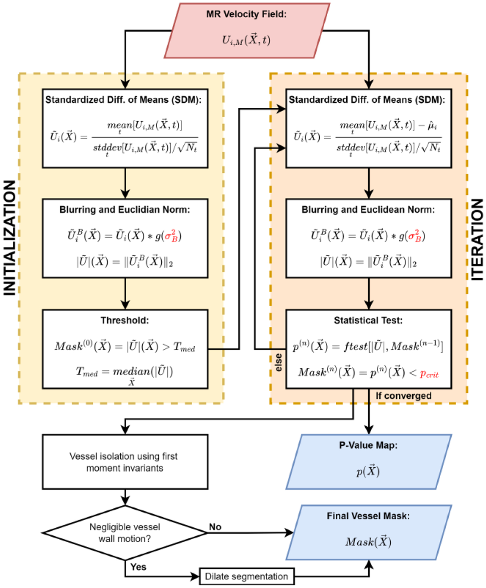
The Standardized Difference of Means (SDM) segmentation algorithm detects voxels with significantly different values of SDM velocity than that of only background noise in the “initialization” and “iterative” steps. Upon convergence of the iterative step, the segmentation is post-processed in the “vessel isolation” step and the optional “dilation” step. The dilation step is included when vessel wall motion is negligible. P-values at all voxels indicate the significance of the statistical test. User-defined input parameters are indicated using red text. Herein, we interchangeably use the terms “segmentation” and “mask”.
The “initialization” step provides a crude approximation of background voxel locations (Section II-B-1). The “iteration” step estimates for each 4D flow MRI dataset according to the measured velocity in background voxels (Section II-B-2). We then infer if the observed value of at each voxel is significantly different than that expected of only noise effects found in the background. Voxels with a significant difference are presumed to exhibit flow and are included in the vessel segmentation. The “vessel isolation” and optional “dilation” steps (Sections II-B-3 and 4) constitute post-processing steps. This work includes the dilation step when vessel wall motion is assumed to be negligible.
1). Initialization
The SDM algorithm is initialized using when calculating . Euclidean norm and blurring operations are applied in the SDM algorithm to improve the detection of voxels with net flow and reduce the SDM velocity variance in background voxels. The blurred SDM velocity is calculated by convolving all components of with a Gaussian blurring kernel according to a user-defined variance . In this work, user-defined parameters are selected according to a grid search technique [51]. We generally recommend setting . For images with low saturation ratio , we recommend as there is already sufficient contrast between flow and background voxels. SR is a measure of the signal in the neighboring background voxels relative to the signal in flow and is a measure of the signal contrast [17]. The magnitude of the blurred SDM velocity, is then evaluated as the SDM velocity vector’s Euclidean norm. The initialized mask, , constitutes all voxels with values greater than the median value of across the entire FOV, .
2). Iteration
The iteration step refines the mask provided by the initialization phase until there are no changes in the segmentation, as shown in Fig. 1. Many steps in the iteration step match those described in Section II-B-1, including the blurring and Euclidean norm operations. However, the iteration phase evaluates after calculating , the arithmetic mean across all time frames and all voxels outside of the past mask iteration, , such that .
We evaluate as the Euclidean norm of the SDM velocity vector for all voxels in the FOV as in the initialization phase; however, we generate the mask for each iteration using an F-test. To perform this statistical test, we first evaluate the F-test statistic, , for each voxel in the FOV:
| (3) |
where and are the regression and error sum of squares, respectively, with degrees of freedom and . We evaluate SSR for each voxel as for . We calculate using all voxels outside of the mask from past iteration, , with where is the number of voxels outside of the mask. We approximate as by assuming the local noise correlations are negligible in comparison to the total noise variance across the FOV. The subtraction of one from results from the calculation of sample means when evaluating the sum of squares values. is approximately equal to as is a measure of the sample variance.
We evaluate the p-value at each voxel, , according to , and . This p-value quantifies the probability that noise effects describe the observed variance of . The mask for the current iteration is generated as p-values that are lower than the user-defined critical p-value, . We recommend setting ; however, should be increased to 0.075 in cases of moving vessel walls, e.g., in the ascending aorta. Herein, is 0.01 in in vitro and in vivo CoW measurements, and 0.075 in in vivo aortic measurements.
We continue the iteration process until the number of voxels in the mask is unchanged. Upon convergence, serves a p-value map for the final SDM segmentation.
3). Vessel Isolation
The “vessel isolation” step in the SDM segmentation algorithm aims to remove erroneous voxels from the converged mask. Despite satisfying the null hypothesis, a relatively small number of background voxels reside far in the tails of the distribution described by (2), exhibiting significant SDM velocity.
To isolate segmented vessels, we first label all separate regions of the converged SDM mask. We break the converged mask up into individual regions, , with being the region index. We define each region as a set of voxels connected according to 6-connectivity using the scipy.ndimage.label method in Python.
We expect vessel regions to have a higher number of voxels and to extend across the FOV, unlike erroneous voxel regions. We quantify this property of each region using the first moment invariant, . We automatically select the regions to retain in the SDM segmentation according to a mean threshold of all values of , .
4). Dilation
The SDM algorithm includes the dilation step to incorporate partial volume (PV) voxels in vessels with negligible wall motion, e.g., cerebral vessels. In vessels which can be assumed to be rigid, PV voxels tend to exhibit lower values of than core flow (CF) voxels because PV voxels partially contain the vessel wall and surrounding voxels composed of stationary medium. Background voxels are assumed to have zero-mean velocity, and blood flow near the vessel wall is generally lower than in CF voxels due to the flow’s viscous effects. In this work, we dilate the segmentation by a single voxel using Python’s skimage.morphology.binary_dilation method. However, vessels with considerable wall motion, e.g., the aorta, exhibit significant flow at the wall due to the moving boundary and do not require segmentation dilation. This optional use of dilation is demonstrated in application of the SDM algorithm to the CoW and thoracic vessels in Section III.
C. In Vitro 4D flow in a Scaled ICA Aneurysm
The SDM segmentation algorithm is applied to in vitro 4D flow MRI measurements in 3D-printed flow phantoms replicating an internal carotid artery (ICA) aneurysm. According to IRB-approved protocol, in vivo 4D flow and TOF MRI data of the cerebral vasculature were acquired at Northwestern University. Two flow phantoms were fabricated, one matching in vivo dimensions (unscaled) and one scaled in all directions by a factor of two (scaled). The flow phantom geometries were generated from TOF data, segmented with ITK-SNAP [52] and post-processed using Geomagic Design software (3D Systems, Rock Hill, SC) to model the aneurysm’s luminal surface. The 1-to-1 and scaled-up 2-to-1 in vitro phantoms were fabricated with a high-resolution ProJet MJP 2500 Plus 3D printer (3D Systems, Rock Hill, SC).
A flow loop was created to conduct in vitro 4D flow measurements of the intra-aneurysmal flow at a steady flow rate. The working fluid was a water-glycerol mixture (60:40 by volume). The Reynolds number in the two in vitro geometries was matched to ensure flow similarity. A gadolinium-based contrast agent was administered for the acquisition of both flow phantom scales. In vitro velocity measurements in both phantoms were acquired at Purdue University’s MRI Facility on a Siemens 3T PRISMA scanner using dual-venc 4D flow MRI, which applies k-t GRAPPA acceleration [53]. Parameters used for each phantom scale are shown in Table II. Additional details of this experiment are provided in our previous work [19].
TABLE II.
Imaging parameters for in vitro scaled aneurysm Studies
| Scale | Vencs (cm/s) | Voxel Size (mm3) | Time Frames | TE, TR (ms) |
|---|---|---|---|---|
| 1-to-1 | 30, 60 | 0.80×0.80×0.80 | 18 | 4.08, 6.78 |
| 2-to-1 | 15, 30 | 0.85×0.85×0.80 | 18 | 4.80, 7.50 |
We apply the SDM segmentation algorithm to the 1-to-1, and 2-to-1 scaled geometries using the 4D flow MRI velocity measurements. In both phantoms, we set the blurring coefficient, , and the critical p-value, . We included the dilation operation when generating the SDM segmentations as the phantoms were printed with a rigid plastic (VisiJet M2R-CL). We compare our SDM segmentation algorithm to segmentations generated using a pseudo-complex difference (PCD) method. PCD segmentations serve as the reference for our SDM algorithm as it does not require model training and is fully automatic when coupled with dynamic thresholding. The PCD algorithm can also be applied to cases with steady flow.
To assess the PCD segmentation, we first evaluate the PCD intensity as defined by Schnell et al. [53]:
| (4) |
where is the signal magnitude of the 4D flow MRI data, and is the speed of the 4D flow MRI measured velocity. is resolved in space and time. We evaluate the 3D resolved only in space by calculating the mean squares with respect to time as Berhane et al. [32].
In typical practice, segmentations are generated from the PCD intensity according to a user-defined threshold or manual segmentation [53]. To eliminate user influence in PCD segmentation generation and promote direct comparisons between the PCD and SDM methods, we automatically threshold the PCD intensity using a triangle threshold. The automatic triangle threshold operation is performed in Python’s scikit-image library using skimage.filters.threshold_triangle.
Since the flow phantoms were 3D-printed, the true vessel geometries are known according to the stereolithography (STL) file used for printing. We determine the accuracy of the SDM and PCD segmentations by registering the true flow phantom geometry to the segmentations using the Coherent Point Drift (CPD) algorithm [54], [55]. Baseline segmentations are assessed by downsampling the high-resolution 3D-printed geometries to the resolution of the 4D flow MRI measurements.
We qualitatively assess the performance of the segmentation methods by comparing the surfaces of the SDM and PCD to that of the benchmark segmentation provided by the phantom geometry. Maps of the SDM velocity and p-values will be generated to demonstrate the method’s sensitivity to regions of flow. Quantitative comparisons will be made using performance metrics described in Section II-F.
D. In vivo 4D flow in the Circle of Willis (CoW)
The performance of the SDM segmentation algorithm will be assessed in the CoW of ten patients, with TOF-based segmentation serving as a benchmark. According to IRB- approved protocol, in vivo 4D flow MRI and TOF data of the cerebral vasculature were acquired at Northwestern University using a Siemens 3T PRISMA scanner (Siemens, Erlangen, Germany). Relevant parameters of the 4D flow MRI data for all ten patients (A-J) are shown in Table III. All CoW patient scans had flip angles of 15 degrees. The TOF voxel sizes for Patients A, E, I, and J were 0.60 × 0.43 × 0.43mm3, 0.60 × 0.27 × 0.27mm3, 0.50 × 0.52 × 0.52mm3, and 0.55 × 0.26 × 0.26mm3, respectively. All other patients had TOF voxel sizes of 0.50 × 0.26 × 0.26mm3. These in vivo data are retrospective routine clinically indicated scans. No contrast agent was administered during the acquisition of the 4D flow or TOF data in any of the patients.
TABLE III.
4D flow MRI parameters for in vivo Studies
| Pat. | Venc(s) (cm/s) | Voxel Size (mm3) | Time Frames | TE, TR (ms) |
|---|---|---|---|---|
| A | 50, 100 | 1.15×1.15×1.20 | 16 | 3.40, 6.10 |
| B | 50, 100 | 1.04×1.04×1.00 | 11 | 3.48, 6.30 |
| C | 50, 100 | 1.15×1.15×1.20 | 8 | 3.39, 6.10 |
| D | 50, 100 | 1.04×1.04×1.20 | 6 | 3.39, 6.10 |
| E | 60, 120 | 0.98×0.98×1.00 | 17 | 3.40, 6.19 |
| f | 50, 100 | 1.15×1.15×1.20 | 16 | 3.39, 6.10 |
| G | 50, 100 | 1.15×1.15×1.20 | 16 | 3.39, 6.10 |
| H | 50, 100 | 0.98×0.98×1.00 | 16 | 3.52, 6.30 |
| I | 60, 120 | 0.98×0.98×1.00 | 19 | 3.40, 6.20 |
| J | 60, 120 | 1.04×1.04×1.00 | 15 | 3.36, 6.10 |
| K | 150 | 2.38×2.38×2.40 | 21 | 2.45, 4.80 |
| L | 150 | 2.50×2.50×2.40 | 15 | 2.43, 4.80 |
| M | 150 | 2.25×2.25×2.40 | 17 | 2.46, 4.90 |
| N | 150 | 2.25×2.25×2.40 | 17 | 2.46, 4.90 |
| O | 150 | 2.25×2.25×2.40 | 16 | 2.43, 4.80 |
The leftmost column indicates the unique identifier for each patient (pat.). Patients A-J and patients K-O correspond to cerebral and aortic 4D flow images, respectively.
The 4D flow images were segmented using the SDM algorithm for and in all ten patients. Hyperparameters were selected using a grid search technique and the dilation operation was included as wall motion is assumed to be negligible in the CoW [44], [51]. The Appendix presents the grid search and ablation study conducted for a Patient H. The PCD segmentations were generated using the procedure described in Section II-C.
The TOF images were segmented as in Section II-C to serve as a reference for assessing SDM and PCD segmentation accuracy [52]. We determine the accuracy of the SDM and PCD segmentations by registering the TOF data to the segmentations using the CPD algorithm as in Section II-C. The registered TOF segmentations are then downsampled to the resolution of the 4D flow MRI measurements. We limited the downsampled TOF to the CoW by removing other vessels passing through the edge of the FOV.
Patient H’s CoW contains a 2.1 cm diameter aneurysm on the right internal carotid artery (ICA). The segmentation of the slow flow in large aneurysms is typically challenging for flow-based segmentation methods [52], and will be used to demonstrate the robustness of the SDM segmentation algorithm. We qualitatively assess the performance of the segmentation methods by comparing the surfaces of the SDM and PCD to the downsampled TOF segmentations in Patient H. Maps of the SDM velocity and p-values found for Patient H were generated to demonstrate the method’s detection of flow regions. Quantitative comparisons across all patients will be made using performance metrics described in Section II-F.
E. In vivo 4D flow in the Aorta
We assess the performance of the SDM segmentation algorithm in the aortas of five patients in comparison to a deep learning algorithm with manual segmentation of the aortas serving as a benchmark. According to IRB-approved protocol, in vivo 4D flow MRI data of the aorta were acquired on a 1.5T MAGNETOM Aera scanner (Siemens, Erlangen, Germany). Relevant parameters of the 4D flow MRI data for all five aortic patients (K-O) are shown in Table III. All patient scans had flip angles of 7 degrees. These in vivo data are retrospective routine clinically indicated scans similar to those described in Section II-D. No contrast agent was administered during the 4D flow MRI acquisition in any of the patients included in this work.
The 4D flow images were segmented using the SDM algorithm for and in all five patients without binary dilation. Hyperparameters were selected using a grid search technique [51]. The dilation operation was not included in thoracic vessels due to aortic wall motion [56]. The Appendix presents the grid search and ablation study conducted for a Patient K. The CNN segmentations were generated using the trained deep learning model described by Berhane et al. [32]. A 3D U-Net network was used with DenseNet-based blocks and implemented using Tensorflow (Google, Mountain View, CA) [57], [58]. A 4D flow-derived phase-contrast MR angiography (PC-MRA) intensity similar to the PCD intensity served as the input for the CNN to generate the segmented images. Additional details of the CNN training and architecture are provided by Berhane et al. [32].
F. Performance Metrics
We quantitatively assess the performance of the predicted segmentations generated by the SDM, PCD and CNN algorithms in reference to the benchmark segmentations. These performance metrics explore the distance between the predicted and benchmark segmentation surfaces and the overlap of the predicted and benchmark segmentation volumes. The benchmark segmentations are provided by the true in vitro geometry, the in vivo TOF segmentations (CoW), or the manual segmentations (aortas).
We evaluate the segmentation accuracy by calculating the minimum distances from each voxel on the benchmark surface to the predicted vessel surface. We express the locations of benchmark and predicted surface segmentation voxels as and , respectively. The minimum distance between and , for all is written as:
| (5) |
As a result, a distribution of is generated for each phantom and patient.
We infer the robustness of segmentation methods by comparing distributions of relative values, . We quantify the similarity between two distributions, and , using f-divergence metrics [59]. In this work, we compare distributions using the Hellinger and Total Variation metrics, both of which are special cases of f-divergence.
The Hellinger distance metric, , is quantified as , where is the summation across all probability mass function bins. The Total Variation distance metric, , is quantified as the supremum absolute difference between the two distributions, . Lower values of and indicate that the distributions demonstrate greater similarity.
We evaluate the predicted positives (PP) and predicted negatives (PN) from the SDM, PCD, or CNN segmentation volumes to evaluate overlap metrics. We also evaluate benchmark positives (BP), and benchmark negatives (BN) assessed using the benchmark in vitro geometry, in vivo TOF, or in vivo manual segmentations. Using these predicted and benchmark segmentations, we assess the number of true positives (TP), false positives (FP), false negatives (FN), and true negatives (TN). Table IV shows that these quantities are evaluated as the intersection of the appropriate predicted and benchmark segmentations.
TABLE IV.
Segmentation Performance Metrics
| Metric | Definition |
|---|---|
| True Positives | TP = PP ∩ BP |
| False Negatives | FN = PN ∩ BP |
| False Positives | FP = PP ∩ BN |
| True Negatives | TN = PN ∩ BN |
| Sensitivity | Sen = TP/BP |
| Specificity | Spec = TN/BN |
| Precision | Prec = TP/PP |
| Negative Predictive Value | NPV = TN/PN |
| Balanced Accuracy | Bal Acc = (Sen/Spec)/2 |
| Dice Score | DSC = 2 * TP(PPv+BP) |
Performance metrics assessed from the predicted positives (PP), benchmark positives (BP), predicted negatives (PN), and benchmark negatives (BN). We assess the Dice score using the valid predicted positives .
We look to calculate relative quantities so the performance of the segmentation algorithms can be directly compared across in vitro geometry scales and in vivo patient data. To achieve this, we evaluate the sensitivity (Sen.), specificity (Spec.), precision (Prec.), negative predictive value (NPV), balanced accuracy (Bal. Acc.), and Dice score (DSC) as defined in Table IV.
Performance metrics assessed from the predicted positives (PP), benchmark positives (BP), predicted negatives (PN), and benchmark negatives (BN). We assess the Dice score using the valid predicted positives .
The balanced accuracy is evaluated in cases where the performance in assessing negatives and positives should be equally represented [60]. Our datasets generally contain far more benchmark negatives than benchmark positives because blood vessels make up a small fraction of the overall image volume.
We evaluate the Dice score (DSC) using the “valid predicted positives” . We evaluate the valid predicted positives as the predicted segmentation that lies inside a restricted region of the FOV. This restricted region is determined by dilating the baseline segmentation by three voxels in the 1-to-1 in vitro case, and all in vivo cases. For the 2-to-1 flow phantom we dilate by six voxels to maintain consistent scaling between the 1-to-1 and 2-to-1 measurements. Considering predicted voxels only inside the dilated baseline segmentation provides a balance between benchmark negatives and benchmark positives (~1.5 to 1 ratio). Additionally, the restricted region mitigates penalizing the predicted segmentation methods for assessing veins and other vessels commonly omitted in the baseline segmentations.
III. RESULTS
We compare the SDM segmentation method to the PCD and CNN approaches across a range of flow and imaging conditions. Sections III-A, III-B and III-C present results in in vitro aneurysm phantoms, in vivo CoW, and in vivo aorta measurements, respectively. Section III-D collectively compares the segmentation results presented in Sections III-A through III-C to assess the robustness of all segmentation methods.
A. In Vitro 4D flow in a Scaled ICA Aneurysm
The SDM algorithm segments voxels which exhibit significantly high values of SDM velocity. Fig. 2 plots cross-sections of the SDM velocity magnitude and p-values in the in vitro flow phantoms. We report log p-values to best express the full range of p-values in the vessels. These cross-sectional planes cut through the ICA inlet, ICA outlet, and aneurysm sac. The green outline indicates the surface of the downsampled benchmark segmentation of the 3D-printed flow phantoms.
Fig. 2:
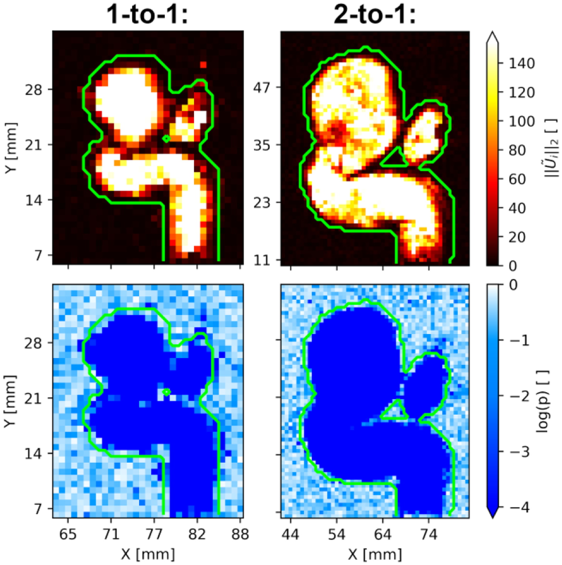
Maps of SDM velocity magnitude (top panels) and log p-values (bottom panels) associated with each voxel in a cross-sectional slice through the 1-to-1 (left panels) and 2-to-1 (right panels) phantom geometries. The outer boundaries of the benchmark segmentation are shown in green.
In both the 1-to-1 and 2-to-1 flow phantoms, the SDM magnitudes are much higher inside the phantom geometries than outside. This high contrast of the SDM velocity produces very low p-values inside the segmentation. This is demonstrated in Fig. 2 by the p-values being less than inside the segmentation. We observe that SDM magnitude values decrease as the voxels in the flow approach the wall of the flow phantom. This leads to increased p-values near the wall as well. Voxels near the wall are partially composed of tissue and contain slower flow due to viscous friction with the wall.
Fig. 3 shows the PCD (panels a and b) and SDM segmentations (panels c and d) in reference to the benchmark flow phantom geometries in the 1-to-1 (panels a and c) and 2-to-1 (panels b and d) geometries. Red surfaces indicate the PCD or SDM segmentations, and the blue wireframes show the true geometry.
Fig. 3:
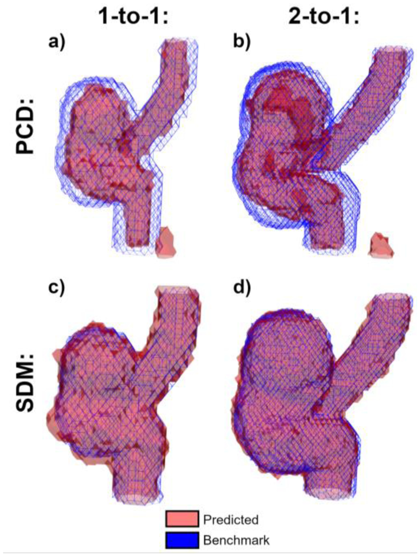
Segmentation boundaries for the 1-to-1 (a, c) and 2-to-1 (b, d) in vitro phantom comparing (a, b) and (c, d) methods to the benchmark phantom geometries. PCD and SDM segmentations are shown as red surfaces, and the benchmark geometry is shown using blue wireframes.
In both the 1-to-1 and 2-to-1 datasets, the PCD segmentation omits many near-wall voxels which are captured in the SDM segmentations. Furthermore, the PCD segmentation of the 2-to-1 phantom (panel b) misses a region in the center of the aneurysm sac. In contrast, these voxels are included in the SDM segmentation (panel d). Panels a and b show that the PCD algorithm erroneously includes a segmented region to the right of the ICA inlet, resulting from a phase wrapping artifact. The SDM algorithm correctly omits this artifact.
We quantitatively assess the discrepancy between the surfaces of the predicted and benchmark segmentation using the minimum distance performance metric, , described in Section II-F. To promote comparison of minimum distances across segmentations, we non-dimensionalize using the L2-norm of the acquisition’s voxel size, , where is the 3D voxel size. Fig. 4 plots the distributions of according to the flow phantom scale and segmentation method.
Fig. 4:
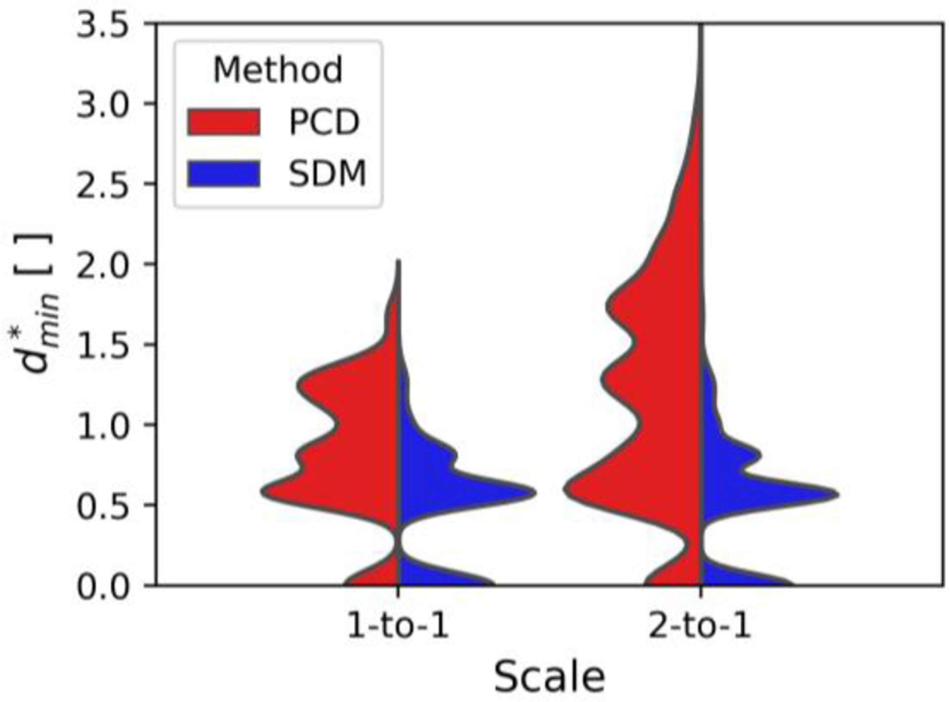
Split violin plots comparing the minimum relative distance between predicted and benchmark flow phantom segmentations. The flow phantom scale is shown according to the position on the x-axis, and the method to predict the segmentation is shown on opposite sides of the split violin plot.
The violin plots exhibit many peaks as is a discrete variable. The SDM segmentation surfaces are equidistant or closer to the benchmark segmentation in 77.8% of voxels compared to the PCD surfaces. Furthermore, when comparing different phantom scales, the SDM method produces similar distributions of . Contrastingly, the PCD method exhibits a greater spread of in the 2-to-1 phantom compared to 1-to-1. These findings are quantitatively expressed in Table V, which presents the median and root mean square (RMS) values according to the segmentation method and in vitro geometry scale.
TABLE V.
In Vitro Minimum Relative Distance
| PCD | SDM | |||
|---|---|---|---|---|
| Scale | MEDIAN | RMS | Median | RMS |
| 1-to-1 | 0.82 | 0.92 | 0.58 | 0.60 |
| 2-to-1 | 1.18 | 1.38 | 0.55 | 0.66 |
| Total | 1.00 | 1.29 | 0.58 | 0.65 |
The SDM method exhibits lower median and RMS values than the PCD method for both in vitro scales. The SDM method shows more conserved median and RMS values between the scaled geometries with differences of 0.03 and 0.06, respectively, as compared to the PCD method, which exhibited differences of 0.36 and 0.46. Overall, the SDM segmentations exhibit medians and RMS values, respectively, 42.0% and 49.6% lower than the PCD approach.
We explore the SDM method’s performance in assessing the full segmentation volume using overlap metrics. Table VI presents these metrics according to the in vitro phantom scale and segmentation method.
TABLE VI.
In Vitro Overlap Metrics
| PCD | SDM | |||
|---|---|---|---|---|
| Metric | 1-TO-1 | 2-TO-1 | 1-TO-1 | 2-TO-1 |
| Sen. | 49.77% | 49.24% | 97.67% | 97.32% |
| Spec. | 99.95% | 99.89% | 98.53% | 98.29% |
| Prec. | 97.23% | 96.85% | 69.05% | 79.67% |
| npv | 98.35% | 96.60% | 99.92% | 99.81% |
| Bal. Acc | 74.86% | 74.56% | 98.07% | 97.80% |
| DSC | 65.88% | 65.54% | 82.14% | 91.25% |
Performance values are bolded when they are decidedly higher than alternate segmentation method.
The SDM method demonstrates a 47.83% and 48.08% increase in sensitivity compared to the PCD method for the 1-to-1 and 2-to-1 phantom scales, respectively. The SDM method indicates a 23.24% and 23.34% increase in balanced accuracy compared to the PCD method for the 1-to-1 and 2-to-1 phantom scales, respectively. Compared to the PCD method, the SDM algorithm achieves a 16.26% and 25.71% increase in the Dice score for the 1-to-1 and 2-to-1 phantoms, respectively. However, Table VI shows that the SDM method is less precise than the PCD segmentation algorithm in this in vitro study. Values of NPV and specificity are similar across segmentation methods and aneurysm phantom scales.
B. In vivo 4D flow in the CoW
The performance of the SDM method is assessed in vivo in the cerebral vasculature of ten patients. Fig. 5 shows the SDM velocity magnitude and p-values in a cross-section of Patient H’s CoW. Fig. 5a depicts the location of this cross-section as a green plane that passes through both ICAs, middle cerebral arteries (MCAs), and the 2.1 cm diameter aneurysm located on the right ICA. The green outline indicates the surface of the downsampled TOF segmentation in Figs. 5b and 5c.
Fig. 5:
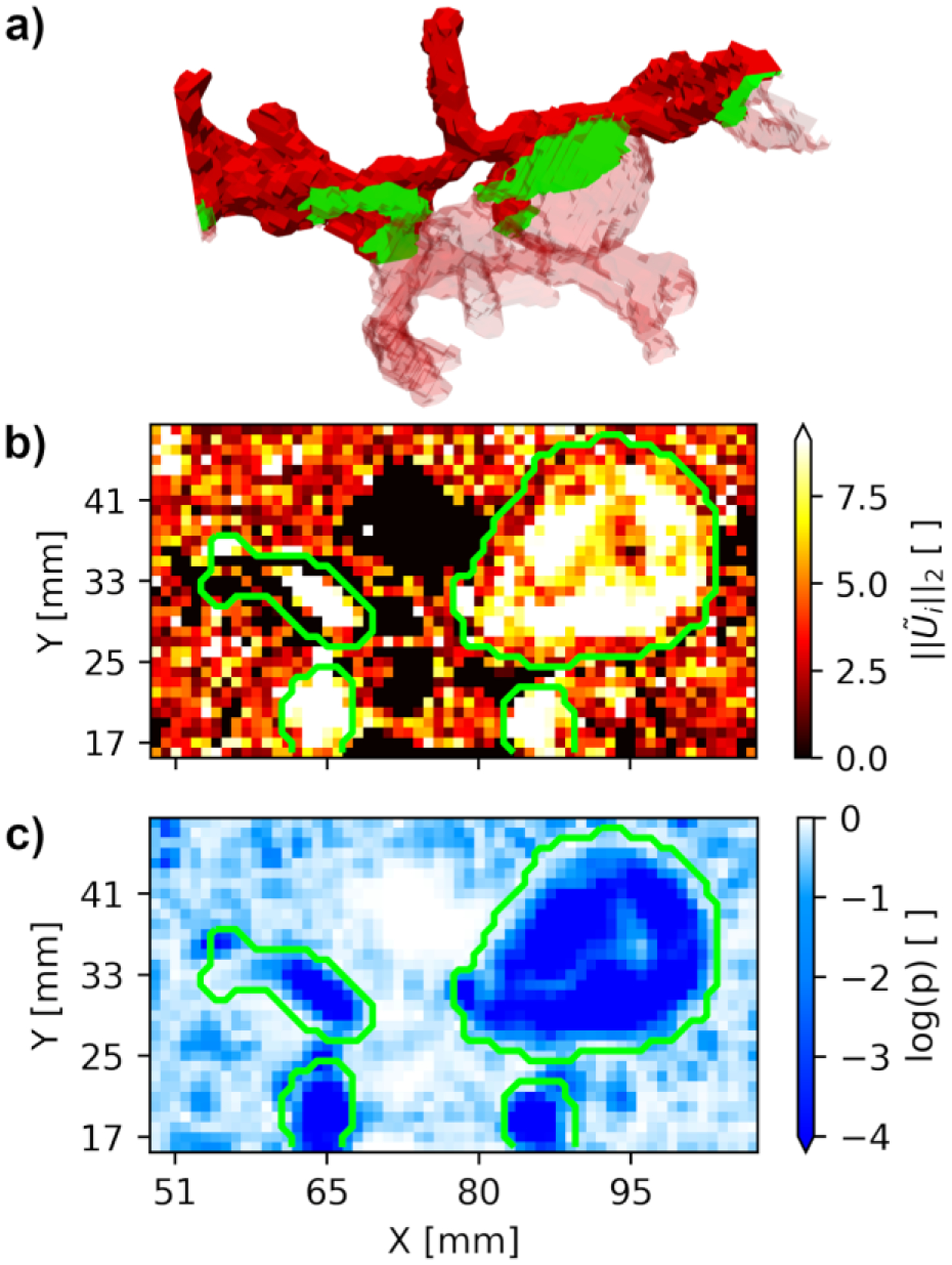
Cross-section through Patient H’s Circle of Willis (panel a) passing through both ICAs, MCAs, and the 2.1 cm diameter aneurysm located on the right ICA. The SDM velocity magnitude and log p-values along this cross-section are shown in panels b and c, respectively. The outer boundaries of the TOF segmentation are shown in green.
The SDM magnitude in Fig. 5b appears higher within the TOF segmentation than in the surrounding background voxels. These high SDM values correspond to regions of low p-values inside the segmentation (Fig. 5c). SDM magnitude values decrease as the voxels in the flow approach the vessel walls. This leads to increased p-values near the wall. The intra-aneurysmal voxels exhibit lower SDM values at with a trail of low values extending to . This trail of low SDM values corresponds to higher p-values shown in Fig. 5c.
Fig. 6a shows the PCD segmentation in reference to the downsampled TOF segmentation. The SDM segmentation and TOF segmentation are shown in Fig. 6b. The PCD segmentation omits many voxels near the wall and most of the voxels in the aneurysm sac are excluded from the segmentation. Contrastingly, most of these near-wall and intra-aneurysmal voxels are captured by the SDM algorithm. This suggests that the SDM method is more sensitive to slow blood flow regions than the PCD method. The PCD method also includes many background voxels with high noise, omitted by the SDM algorithm. The SDM segmentation includes vessels that are not part of the TOF segmentation. These vessels are likely veins that are suppressed during the TOF acquisition [61].
Fig. 6:
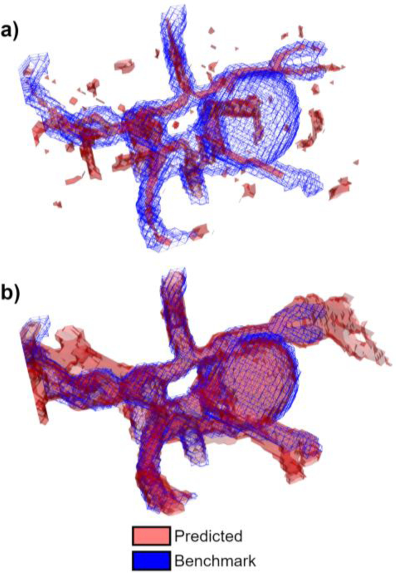
Segmentation boundaries for Patient H with a 2.1 cm diameter aneurysm on the right ICA. Panel a) compares the PCD method and TOF, and panel b) compares the SDM method and TOF. PCD and SDM segmentations are shown using red surfaces, and TOF is shown using blue wireframes.
Fig. 7 quantitatively expresses the differences between the PCD and SDM segmentation surfaces compared to TOF for all ten patients. As in Section III-A, surface segmentation performance is assessed using the minimum relative distance between the benchmark and predicted segmentations, .
Fig.7:
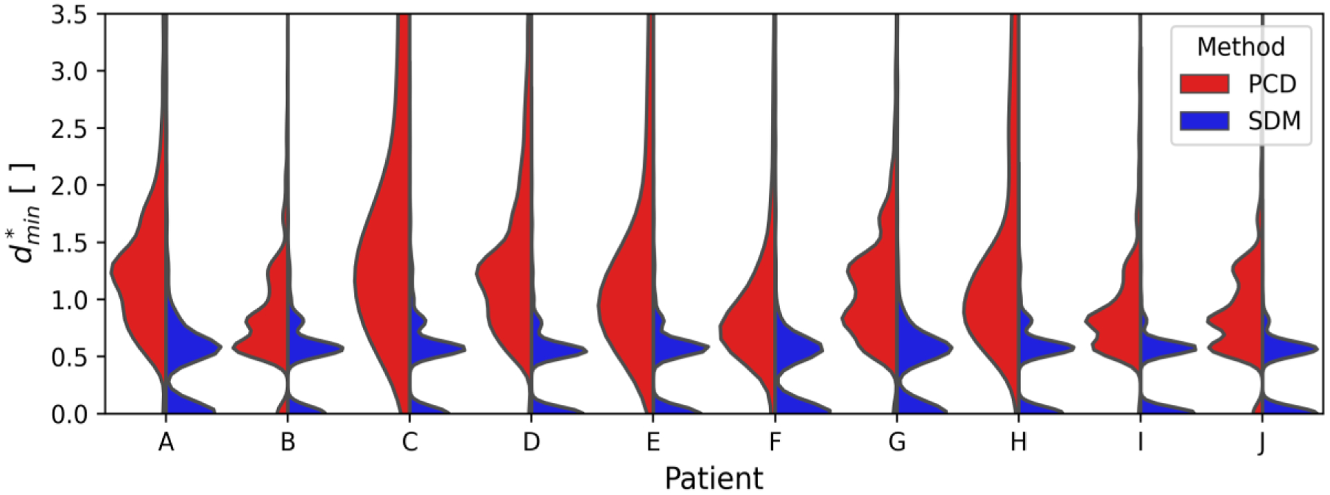
Splitviolin plots comparing the minimum relative distance between predicted and benchmarkCircle of Willis segmentations. The patient identifieris shown according to the position on the x-axis and the method to predict the segmentation is shown on opposite sides of the split violin plot.
The SDM segmentation method demonstrates lower values of compared the PCD method across all ten patients. The SDM segmentation surfaces are equidistant or closer to the benchmark segmentation in 93.5% of voxels compared to the PCD surfaces. Moreover, extended upper tails observed for the PCD method are absent from the SDM segmentations. Median and RMS values for each distribution shown in Fig. 7 are presented in Table VII.
TABLE VII.
In Vivo Minimum Relative Distance in CoW Measurements
| PCD | SDM | |||
|---|---|---|---|---|
| Patient | MEDIAN | RMS | Median | RMS |
| A | 1.27 | 1.70 | 0.57 | 0.76 |
| B | 0.81 | 1.00 | 0.56 | 0.58 |
| C | 1.70 | 3.29 | 0.57 | 0.63 |
| D | 1.23 | 1.70 | 0.55 | 0.53 |
| E | 1.15 | 2.75 | 0.57 | 0.56 |
| f | 0.82 | 1.53 | 0.57 | 0.67 |
| G | 1.00 | 1.29 | 0.57 | 0.70 |
| H | 1.17 | 2.19 | 0.57 | 0.54 |
| I | 0.82 | 1.10 | 0.57 | 0.47 |
| J | 0.81 | 1.00 | 0.56 | 0.45 |
| Total | 1.14 | 2.10 | 0.56 | 0.59 |
For each patient, the SDM method exhibits lower median and RMS values than the PCD method. Furthermore, the median and RMS values are more similar using the SDM method than the PCD method, which suggests fewer outliers. The range of median values for the SDM and PCD methods is 0.02 and 0.89, respectively. The range of RMS values is 0.31 and 2.29 for the SDM and PCD methods, respectively. Overall, the median and RMS values of are 50.9% and 71.9% lower in vivo for SDM segmentations than those from the PCD method.
Table VIII presents the overlap metrics according to the segmentation method for all ten patients with cerebral measurements. The SDM method demonstrates a increase in sensitivity, a 32.58% increase in balanced accuracy and a 48.32% increase in the Dice score compared to the PCD method. The specificity of the two methods is similar. Calculations of precision and NPV are not valid using TOF as a reference as this imaging modality does not capture veins when presaturation pulses are applied [52].
TABLE VIII.
In Vivo Overlap Metrics for all CoW Measurements
| Metric | PCD | SDM |
|---|---|---|
| Sen. | 16.49% | 86.63% |
| Spec. | 99.71% | 94.73% |
| Bal. Acc | 58.10% | 90.68% |
| DSC | 28.15% | 76.47% |
Performance values are bolded when they are decidedly higher than alternate segmentation method.
C. in vivo 4D flow in the Aorta
The performance of the SDM method is assessed for in vivo 4D flow in the thoracic vasculature of five patients. Fig. 8 shows the SDM velocity magnitude (left panel) and p-values (right panel) in a sagittal cross-section of Patient K’s aorta. The outline of the baseline manual segmentation is shown in green for both the SDM magnitude and log p-value cross-sections. We plot the log p-values to depict the dynamic range of this parameter.
Fig. 8:
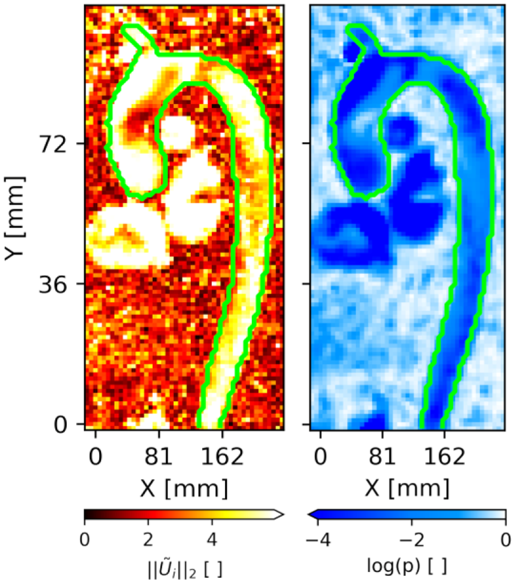
Sagittal cross-section in Patient K passing through both the aorta (Ao), brachiocephalic trunk (BCT), pulmonary artery (PA), left ventricle (LV) and right ventricle (RV). The SDM velocity magnitude and log p-values along this cross-section are shown in the left and right panels, respectively. The outer boundaries of the manual segmentation are shown in green.
The SDM magnitude in Fig. 8 is generally higher inside of the baseline segmentation compared to many of the surrounding background voxels. However, we observe particularly low SDM magnitude values in the ascending aorta near which corresponds to elevated p-values in the same region. The manual segmentation was performed for the aorta and proximal brachiocephalic trunk (BCT) only. For all aortic patients, we note that the vessels captured by the CNN segmentations match the few vessels included in the manual benchmark segmentations. In addition to segmenting the aorta and BCT, the SDM method also captures the pulmonary artery, left brachiocephalic vein and chambers of the heart in this p-value cross-section. As in the ascending aorta, we also observe low SDM values at the center of the heart chambers. The SDM algorithm depiction of these vessels omitted by the manual and CNN segmentations demonstrates the generalizability of the SDM method across vascular territories.
We quantify the performance of the CNN and SDM methods in assessing the surface of the baseline segmentations. As in Sections III-A and III-B, the methods’ performance in assessing the vessel surface is quantified using the minimum relative distance between the benchmark and predicted segmentations, . The minimum relative distance distributions for the CNN and SDM segmentations are shown in Fig. 9 for all aorta cases.
Fig. 9:
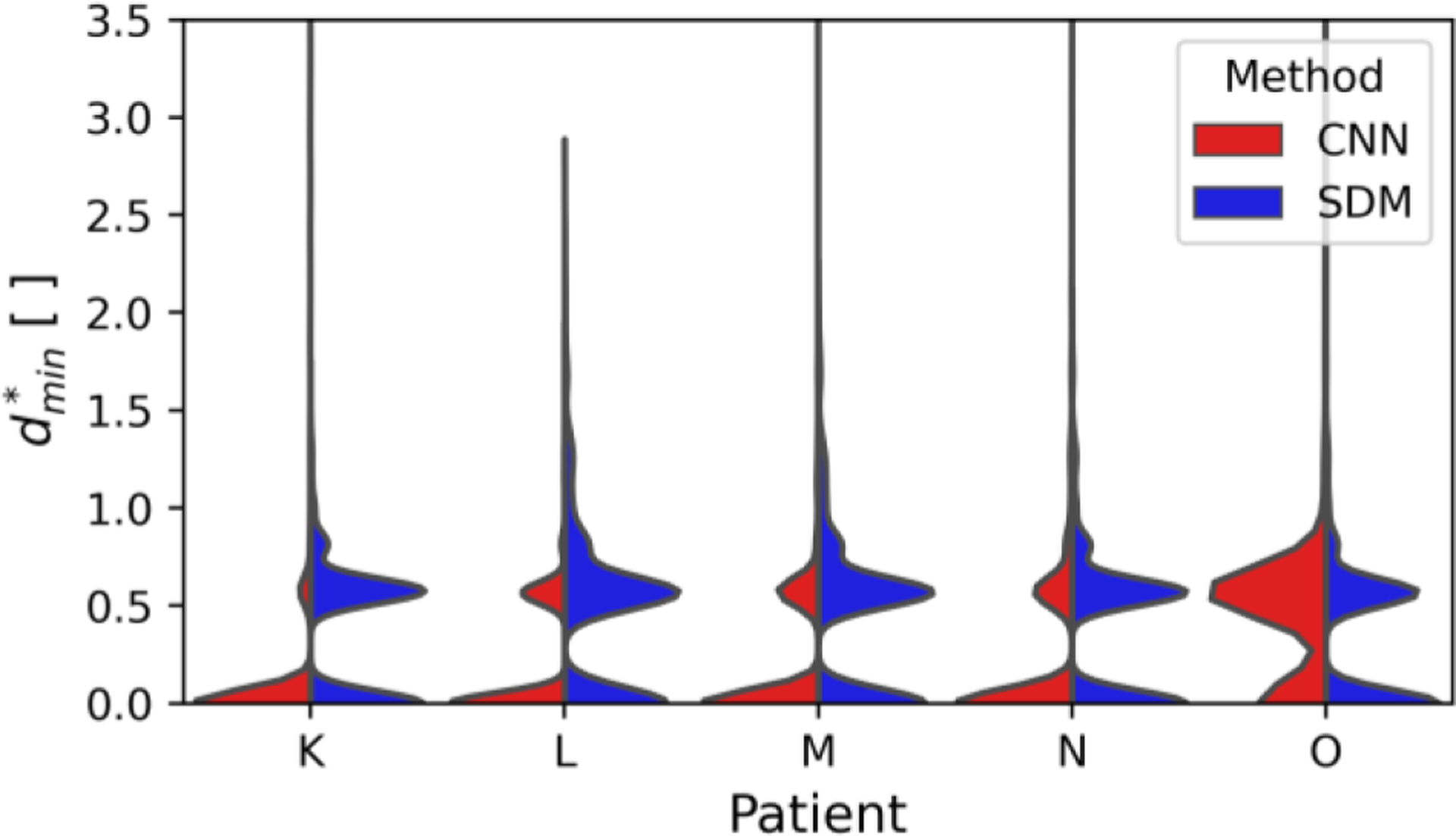
Split violin plots comparing the minimum relative distance between predicted and benchmark aorta segmentations. The patient identifier is shown on the x-axis and the segmentation method is shown on opposite sides of the split violin plot.
Fig. 9 indicates that the error in assessing the vessel surface is largely within a single voxel distance for both methods. The RMS minimum relative distances across all aorta cases are 0.50 and 0.54 for the CNN and SDM methods, respectively. Both methods provide comparable results across all aortic patients.
Table IX presents the overlap metrics according to the segmentation method for all five aortic patients. The CNN method outperforms the SDM method as measured by the overlap metrics. Namely, the CNN segmentations demonstrate a 21.36% increase in specificity, a 12.89% increase in balanced accuracy and a 14.82% increase in the Dice score compared to the SDM method. The sensitivity of the two methods is similar. We note that the Dice score of 93.20% found in Table IX for the CNN segmentations falls within the interquartile range (91.6–95.8%) reported by Berhane et al. for their control cases [32].
TABLE IX.
In Vivo Overlap Metrics for all aortic measurements
| Metric | CNN | SDM |
|---|---|---|
| Sen. | 90.62% | 86.21% |
| Spec. | 99.56% | 78.20% |
| Bal. Acc | 95.09% | 82.20% |
| DSC | 93.20% | 78.38% |
Performance values are bolded when they are decidedly higher than alternate segmentation method.
D. Assessing Segmentation Robustness
The robustness of the SDM segmentation method is assessed by comparing all in vitro scaled aneurysm, in vivo CoW, and in vivo aorta relative minimum distance distributions. We quantify the difference between two distributions using f-divergence metrics (Hellinger and Total Variation distances) as described in Section II-F. Lower values of Hellinger and Total Variation distances express greater similarity between the two distributions. All 17 cases’ distributions are compared pairwise, i.e., a total of 289 comparisons are performed. These metrics are quantified across all SDM segmentations and across all alternative segmentations. Here, PCD and CNN constitute the alternative segmentation methods and PCD or CNN is chosen depending on the data category, e.g., aorta data uses CNN whereas CoW uses PCD.
Fig. 10 presents the Hellinger and Total Variation metrics using the PCD or CNN methods in the left panels, and the metrics using the SDM method in the right panels. We denote the boundaries between different data categories (in vitro phantoms, CoW, and aorta cases) using solid red lines. We abbreviate “phantom” and “aorta” as “ph” and “Ao”, respectively.
Fig. 10:
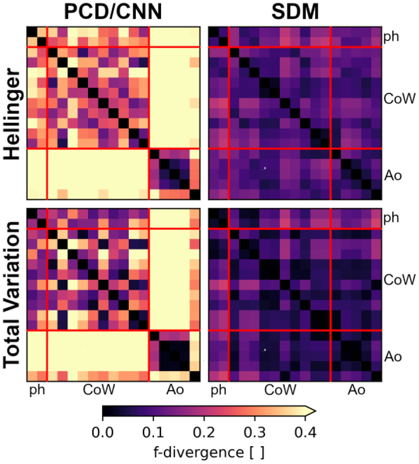
Pairwise comparisons between all 17 cases’ minimum relative distance distributions using f-divergence metrics. Lower f-divergence values indicate greater similarity between distributions. The f-divergence is quantified using the Hellinger (top panels) and Total Variation (bottom panels) metrics, using the SDM segmentation method (right panel) or alternative methods (left panels). The alternative methods include either the PCD or CNN approaches. The boundaries between data categories, i.e., in vitro phantoms (ph), in vivo Circle of Willis (CoW), or in vivo aorta (Ao), are indicated using solid red lines.
Overall, we qualitatively observe that the SDM method demonstrates lower values of and than the PCD/CNN approaches. This is observed both within individual data categories, e.g., between different aorta cases, and across different data categories, e.g., between aorta and CoW cases. We see particularly large differences in distributions when comparing the CNN segmentations to the PCD segmentations.
Table X quantitatively summarizes the observations presented in Fig. 10 using “aggregate” f-divergence metrics. We evaluate the aggregate Hellinger distance metric, , as the RMS value across a given set of pairwise comparisons. We evaluate the aggregate Total Variation distance metric, , as the maximum TV value. We do not consider comparisons between the same distribution when calculating aggregate metrics.
TABLE X.
Aggregate F-Divergence METRICS COmparing Minimum Relative DistANCE DiStributions ACrOSS All DATASETS
| PCD/CNN | SDM | |||
|---|---|---|---|---|
| Type | HAGG | TVAGG | HAGG | TVAGG |
| In vitro ph. | 0.353 | 0.174 | 0.081 | 0.033 |
| CoW | 0.267 | 0.479 | 0.107 | 0.174 |
| Aorta | 0.235 | 0.565 | 0.086 | 0.116 |
| All | 0.468 | 0.882 | 0.115 | 0.227 |
Aggregate (AGG) values are bolded when they are decidedly lower than alternate segmentation method(s). Lower aggregate values indicate greater similarity across relative minimum distance distributions.
We observe that both the Hellinger and Total Variation metrics are lower within all three categories and across all pairwise comparisons when using the SDM method. In vitro, we observe a 4.4- and 5.3-fold reduction in and , respectively, when segmenting using the SDM method. We report a 2.5- and 2.8-fold reduction of and in in vivo CoW measurements for the SDM approach. Compared to CNN segmentations, the SDM method reports a 2.7- and 4.9-fold reduction in and . These finding suggests that the SDM method produces more consistent distributions of compared to both the PCD and CNN approaches.
IV. DISCUSSION AND CONCLUSION
In this work, we present the SDM velocity as a feature for segmenting 4D flow MRI measurements. We embed the SDM velocity in an iterative algorithm to identify voxels with significant flow effects, which are identified by comparing the level of SDM velocity to that expected from noise effects alone. Upon convergence of the segmentation, erroneously segmented voxels are removed by considering the first moment invariant of each region of connected voxels. Binary dilation is applied when wall motion is negligible. P-values are reported to express the significance of flow effects at all voxels. We compare the SDM method to the PCD algorithm in in vitro and in vivo cerebral flow measurements and to the CNN approach in in vivo aortic data. The 3D-printed in vitro flow phantom geometries and high-resolution in vivo TOF-derived geometries served as the ground truth for assessing the performance of our SDM segmentations and those obtained with PCD. We compare the SDM method to CNN segmentations in five in vivo aortic cases with manual segmentations serving as the ground truth.
The SDM velocity in (1) expresses the ratio of net flow to the pulsatility measured by 4D flow MRI. In background voxels, this SDM velocity follows the zero-mean normal distribution reported in (2). In contrast, voxels with net flow do not follow this same distribution. Figs. 2, 5 and 8 show that voxels inside the benchmark segmentation generally have much higher SDM velocity magnitude values than those outside the segmentation. Our in vitro steady flow experiment demonstrates SDM velocity magnitude values two orders of magnitude higher than those observed in vivo. The in vitro steady flow exhibits very low spread of the measured velocity in time. According to (1), this low pulsatility is predicted to produce higher SDM velocity values than in vivo arterial flow. Tables VI and VIII quantitatively show that the SDM algorithm is more sensitive to voxels with flow than the PCD method in vitro and in vivo.
Figs. 2, 5 and 8 also demonstrate that regions of high SDM velocity have low p-values and vice versa. This relationship between the SDM velocity and p-values is expressed by (3) as serves as the test statistic for evaluating p-values. In vitro and in vivo CoW results indicate that near-wall voxels exhibited less significant flow effects compared to regions in the core of the flow. These less significant flow effects are expected due to the influence of the surrounding stationary medium in the PV voxels and the slower blood flow near the wall. Our algorithm addresses the low significance of flow effects in PV voxels by implementing the dilation step (Section II-B-4). Contrastingly, in vivo aorta results (Fig. 8) demonstrate more comparable SDM velocity values in and PV voxels than in the CoW, supporting the exclusion of the dilation step in the SDM algorithm. The elevated p-values in the center of the aneurysm observed in Fig. 5c, and reduced SDM velocity in the same region in Fig. 5b indicates this is an area with low net flow, suggesting that this is the center of a vortex in the aneurysm. Similarly, Fig. 8 indicates that there are reduced SDM values and elevated p-values in the aortic arch and heart chambers. These findings indicate reversal of the velocity vectors over the course of the cardiac cycle in these locations.
The definition of the SDM velocity in (1) is robust to 4D flow MRI errors and addresses 4D flow’s intra-scan variability (i.e., throughout the FOV). We observe consistent performance of the SDM algorithm in the FOV despite highly variable levels of noise owing to different signal properties of background voxels and variable SNR [27]. Figs. 3 and 6 show that the SDM segmentations better assess near-wall voxels affected by PV effects than the PCD algorithm [17]. Figs. 4 and 7 show that the SDM algorithm presents narrower distributions of compared to PCD segmentations in vitro and in vivo for all ten CoW patients. This demonstrates that the SDM segmentation algorithm more closely represents the vessel’s surface throughout the FOV. Fig. 9 suggests similar performance between the SDM and CNN methods in assessing the vessel wall as most error is within a voxel size. Furthermore, Figs. 3c, 3d, and 6b show that the SDM segmentation correctly segments voxels inside the aneurysms, which were regularly omitted by the PCD algorithm. These findings suggest that the SDM segmentation algorithm is robust to low velocity-to-noise ratios (VNR) as observed in intra-aneurysmal flow [62]. Additionally, Fig. 8 shows that the SDM method captures flow regions characterized by complex flow structures, e.g., heart chambers. The robust nature of the SDM algorithm would enable more accurate computation of hemodynamic metrics, especially those relying on near-wall velocities, e.g., WSS, implicated in several cardiovascular pathologies [63].
The SDM algorithm uses the F-test statistic in (3) to address inter-scan variability caused by differences between patients and 4D flow scan settings. This standardized performance is achieved by dividing the SDM velocity by the observed background noise variance in (3), promoting direct comparison between different 4D flow scans. Sections II-C, II-D and II-E detail the wide range of flow and imaging conditions included in this work. For instance, we explore flow conditions characteristic of cerebral and thoracic vascular territories. Furthermore, this study demonstrates that the SDM method can be applied to both steady flow (in vitro phantoms) and pulsatile flow (CoW and aorta). We also explore segmentation in cases of low resolution (1-to-1 phantom and CoW) and high resolution of flow structures (2-to-1 phantom and aorta). We characterize segmentation performance using different 4D flow MRI sequences and different scanners from different institutions. These sequences include single venc (aorta) and dual venc (in vitro phantoms and CoW) acquisitions. In vitro data were collected at Purdue University using a 3T PRISMA scanner, in vivo CoW 4D flow measurements were collected at Northwestern University using a 3T PRISMA scanner, and in vivo aorta data were collected at Northwestern University using a 1.5T MAGNETOM scanner. This study also includes 4D flow MRI datasets with contrast administration (in vitro phantoms) and without contrast (in vivo CoW and in vivo aorta). Tables II and III show that varying vencs, voxel sizes, time frame counts, and TE/TR values were included in this work. Notably, we consider cases with as many as 21 time frames (Patient K) and as few as 6 time frames (Patient D).
Section III-D compares the SDM segmentation method’s robustness to that of alternative segmentation approaches. Fig. 10 and Table X demonstrate that the SDM method exhibits lower values of f-divergence as measured using the Hellinger and Total Variation metrics. These lower values of f-divergence suggest that the SDM method performs more consistently than alternative segmentation approaches. This consistent performance across 4D flow MRI data characteristics implies that the SDM segmentation method is more robust than other methods when faced with different flow fields, MR equipment or imaging parameters. Qualitative comparisons made between individual dataset’s distributions in Figs. 4, 7, and 9 illustrate the similarity of SDM results across all cases. Tables VIII and IX reinforce our conclusion regarding the SDM method’s robustness in vivo. We observe the sensitivity and Dice score values only differ by 0.42% and 1.91%, in the CoW and aorta data, respectively.
Deep learning methods will not generalize to other vascular territories without retraining, which is a time-consuming and data-intensive process requiring several hundred 4D flow MRI measurements with ground truth references. Moreover, Aviles et al. reported that deep learning networks failed to generalize to data corresponding to the same vascular territory acquired from other institutions and scanners [40]. As a result, we do not expect that the CNN presented in this work could be directly applied to segment CoW data, unlike the SDM method. Furthermore, even after retraining for different territories, advancements in MRI technology (e.g., improved field strength and image reconstruction methods) will likely necessitate intermittent retraining of deep learning networks.
The SDM algorithm segments all flow regions in the FOV, thus requiring further post-processing steps for selecting arterial or veinous vasculature. The SDM algorithm provides a time-averaged representation of the moving structures, such as the heart. However, many other segmentation methods, e.g., CNNs, typically also provide only static segmentations. Furthermore, the SDM method inherently assumes voxels in blood vessels exhibit net flow across the cardiac cycle, . Areas in the vessel with low net flow (e.g., cerebral spinal fluid flow) may be excluded from the SDM segmentation. Since the SDM method segments vessels by comparing net flow effects to background error variances, we expect the SDM method’s performance will be reduced for VNR values less than one. However, it is likely that reduced performance for low VNR values is found across most segmentation methods.
Our results suggest that the algorithm is limited by reduced precision despite yielding increased sensitivity compared to the PCD method. This behavior is not limited to our algorithm and is generally referred to as the “Precision-Recall Tradeoff” in classification methods [64]. The SDM segmentation algorithm’s design prefers low false negatives as opposed to low false positives.
V. Conclusion
This work presents an approach for segmenting vessels in 4D flow MRI measurements based on the SDM velocity. The SDM velocity quantifies the relation of net flow through the voxel to the flow pulsatility. The accuracy of the SDM segmentation algorithm is reported according to p-values at all voxels. Our segmentation algorithm is validated on in vitro 4D flow MRI measurements in flow phantoms and on in vivo 4D flow MRI acquired in the Circle of Willis and thoracic aorta of 15 patients. The SDM algorithm provides a repeatable method to segment vessels across a range of scan settings, imaging conditions, and vascular territories. This consistent performance of the SDM method would enable more accurate computation of hemodynamic metrics, especially those relying on near-wall velocities such as wall shear stress, which have been implicated in various cardiovascular pathologies.
Acknowledgement
We thank Dr. Maria Aristova for her support in collecting imaging data on patients. We also thank Berhane et al. for providing 4D flow MRI aortic measurements and deep learning results.
This work was supported by the National Institutes of Health awards R21 NS106696 and R01 HL115267.
APPENDIX
HYPERPARAMETER SELECTION
We explore the effects of hyperparameter selection and dilation on the quality of the SDM segmentations. These grid search and ablation studies inform hyperparameter selection for in vivo SDM segmentation described in Section II.
The grid search was performed by randomly selecting and from uniform distributions with bounds of [0,3] and [0,0.2], respectively. The ablation study was conducted by randomly choosing whether to perform binary dilation or not. Both options had equal probabilities of being selected. The Dice score was used to identify the optimal settings.
Fig. A.1 presents examples of the hyperparameter study in select patients for the CoW (top panels) and aorta (bottom panels) for cases with dilation (right panels) and without dilation (left panels). Fig. A. 1 presents the findings for Patients H and K in the CoW and aorta, respectively. The results corresponding to a total of ~12,500 SDM segmentations with different settings are presented. We observe binary dilation increases the DSC in the CoW, whereas, excluding binary dilation produces higher DSC values in the aorta.
Fig. A.1:
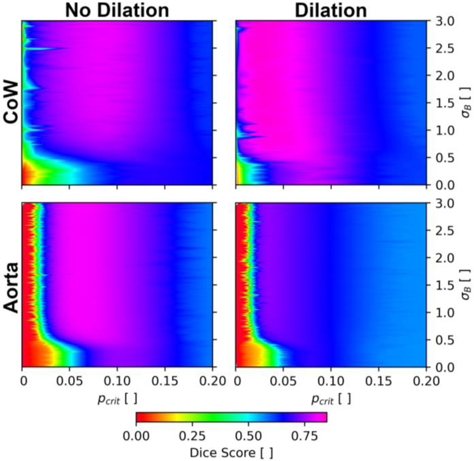
Grid search and ablation study in the Circle of Willis (Patient H) and the aorta (Patient K) exploring the effects of dilation, blurring, and critical p-value on segmentation performance.
Contributor Information
Sean M. Rothenberger, Weldon School of Biomedical Engineering, Purdue University, West Lafayette, IN 47907 USA.
Neal M. Patel, Weldon School of Biomedical Engineering, Purdue University, West Lafayette, IN 47907 USA.
Jiacheng Zhang, School of Mechanical Engineering, Purdue University, West Lafayette, IN 47907 USA.
Susanne Schnell, Institute for Physics, Universität Greifswald, Germany..
Bruce A. Craig, Department of Statistics, Purdue University, West Lafayette, IN 47907 USA.
Sameer A. Ansari, Department of Radiology at the Feinberg School of Medicine, Northwestern University, Chicago, IL 60611 USA.
Michael Markl, Department of Radiology at the Feinberg School of Medicine, Northwestern University, Chicago, IL 60611 USA..
Pavlos P. Vlachos, Weldon School of Biomedical Engineering and School of Mechanical Engineering, Purdue University, West Lafayette, IN 47907 USA
Vitaliy L. Rayz, Weldon School of Biomedical Engineering and School of Mechanical Engineering, Purdue University, West Lafayette, IN 47907 USA
REFERENCES
- [1].Dyverfeldt P, Bissell M, Barker AJ, Bolger AF, Carlhäll CJ, Ebbers T, Francios CJ, Frydrychowicz A, Geiger J, Giese D, Hope MD, Kilner PJ, Kozerke S, Myerson S, Neubauer S, Wieben O, and Markl M, “4D flow cardiovascular magnetic resonance consensus statement,” Journal of Cardiovascular Magnetic Resonance, vol. 17, no. 1, Aug. 2015. [DOI] [PMC free article] [PubMed] [Google Scholar]
- [2].Stankovic Z, Allen BD, Garcia J, Jarvis KB, and Markl M, “4D flow imaging with MRI,” vol. 4, no. 2, pp. 120,2014. [DOI] [PMC free article] [PubMed] [Google Scholar]
- [3].Garcia J, Barker AJ, and Markl M, “The Role of Imaging of Flow Patterns by 4D Flow MRI in Aortic Stenosis,” JACC: Cardiovascular Imaging, vol. 12, no. 2. Elsevier Inc., pp. 252–266, 01-Feb-2019. [DOI] [PubMed] [Google Scholar]
- [4].Markl M, “Techniques in the Assessment of Cardiovascular Blood Flow and Velocity,” 2019, pp. 113125.
- [5].Schnell S, Ansari SA, Vakil P, Wasielewski M, Carr ML, Hurley MC, Bendok BR, Batjer H, Carroll TJ, Carr J, and Markl M, “Three-dimensional hemodynamics in intracranial aneurysms: Influence of size and morphology,” Journal of Magnetic Resonance Imaging, vol. 39, no. 1, pp. 120–131, Jan. 2014. [DOI] [PMC free article] [PubMed] [Google Scholar]
- [6].Morgan AG, Thrippleton MJ, Wardlaw JM, and Marshall I, “4D flow MRI for non-invasive measurement of blood flow in the brain: A systematic review,” Journal of Cerebral Blood Flow and Metabolism. SAGE Publications Ltd, 01-Feb-2020. [DOI] [PMC free article] [PubMed] [Google Scholar]
- [7].Hope TA, Hope MD, Purcell DD, von Morze C, Vigneron DB, Alley MT, and Dillon WP, “Evaluation of intracranial stenoses and aneurysms with accelerated 4D flow,” Magn Reson Imaging, vol. 28, no. 1, pp. 41–46, Jan. 2010. [DOI] [PubMed] [Google Scholar]
- [8].Isoda H, Ohkura Y, Kosugi T, Hirano M, Takeda H, Hiramatsu H, Yamashita S, Takehara Y, Alley MT, Bammer R, Pelc NJ, Namba H, and Sakahara H, “in vivo hemodynamic analysis of intracranial aneurysms obtained by magnetic resonance fluid dynamics (MRFD) based on time-resolved three-dimensional phase-contrast MRI,” Neuroradiology, vol. 52, no. 10, pp. 921–928, 2010. [DOI] [PubMed] [Google Scholar]
- [9].Libby P, Ridker PM, and Maseri A, “Inflammation and atherosclerosis,” Circulation, vol. 105, no. 9, pp. 1135–1143, Mar. 2002. [DOI] [PubMed] [Google Scholar]
- [10].John K, Rauh A, Bruschewski M, and Grundmann S, “Towards Analyzing the Influence of Measurement Errors in Magnetic Resonance Imaging of Fluid Flows,” Acta Cybernetica, vol. 24, no. 3, pp. 343–372, Mar. 2020. [Google Scholar]
- [11].O’brien KR, Cowan BR, Jain M, Stewart RAH, Kerr AJ, and Young AA, “MRI Phase Contrast Velocity and Flow Errors in Turbulent Stenotic Jets,” J. Magn. Reson. Imaging, vol. 28, pp. 210–218, 2008. [DOI] [PubMed] [Google Scholar]
- [12].Wolf RL, Ehman RL, Riederer SJ, and Rossman PJ, “Analysis of Systematic and Random Error in MR Volumetric Flow Measurements,” Magn Reson Med, 1993. [DOI] [PubMed] [Google Scholar]
- [13].Yavuz Ilik S, Otani T, Yamada S, Watanabe Y, and Wada S, “A subject-specific assessment of measurement errors and their correction in cerebrospinal fluid velocity maps using 4D flow MRI,” Magn Reson Med, Dec. 2021. [DOI] [PubMed] [Google Scholar]
- [14].Pelc N, Sommer F, Li K, Brosnan T, Herfkens R, and Enzmann D, “Quantitative magnetic resonance flow imaging.,” Magn Reson Q, vol. 10, pp. 125–147, 1994. [PubMed] [Google Scholar]
- [15].Brindise MC, Rothenberger S, Dickerhoff B, Schnell S, Markl M, Saloner D, Rayz VL, and Vlachos PP, “Multi-modality cerebral aneurysm haemodynamic analysis: in vivo 4D flow MRI, in vitro volumetric particle velocimetry and in silico computational fluid dynamics,” J R Soc Interface, vol. 16, no. 158, 2019. [DOI] [PMC free article] [PubMed] [Google Scholar]
- [16].Tang C, Blatter DD, and Parker DL, “Correction of partial-volume effects in phase-contrast flow measurements,” Journal of Magnetic Resonance Imaging, vol. 5, no. 2, pp. 175–180, 1995. [DOI] [PubMed] [Google Scholar]
- [17].Tang C, Blatter DD, and Parker DL, “Accuracy of phase-contrast flow measurements in the presence of partial-volume effects.,” J Magn Reson Imaging, vol. 3, no. 2, pp. 377–85,1993. [DOI] [PubMed] [Google Scholar]
- [18].Jiang J, Kokeny P, Ying W, Magnano C, Zivadinov R, and Mark Haacke E, “Quantifying errors in flow measurement using phase contrast magnetic resonance imaging: Comparison of several boundary detection methods,” Magn Reson Imaging, vol. 33, no. 2, pp. 185193, Feb. 2015. [DOI] [PMC free article] [PubMed] [Google Scholar]
- [19].Rothenberger SM, Zhang J, Brindise MC, Schnell S, Mark1 M, Vlachos PP, and Rayz VL, “Modeling Bias Error in 4D flow MRI Velocity Measurements,” IEEE Trans Med Imaging, p. 1, 2022. [DOI] [PMC free article] [PubMed] [Google Scholar]
- [20].Zhang J, Brindise MC, Rothenberger S, Schnell S, Markl M, Saloner D, Rayz VL, and Vlachos PP, “44 Flow MRI Pressure Estimation Using Velocity Measurement-Error based Weighted Least-Squares,” IEEE Trans Med Imaging, pp. 1–1, Nov. 2019. [DOI] [PMC free article] [PubMed] [Google Scholar]
- [21].Juffermans JF, Westenberg JJM, van den Boogaard PJ, Roest AAW, van Assen HC, van der Palen RLF, and Lamb HJ, “Reproducibility of Aorta Segmentation on 4D Flow MRI in Healthy Volunteers,” Journal of Magnetic Resonance Imaging, vol. 53, no. 4, pp. 1268–1279, Apr. 2021. [DOI] [PMC free article] [PubMed] [Google Scholar]
- [22].Schrauben E, Ambarki K, Spaak E, Malm J, Wieben O, and Eklund A, “Fast 4D flow MRI intracranial segmentation and quantification in tortuous arteries,” Journal of Magnetic Resonance Imaging, vol. 42, no. 5, pp. 1458–1464, Nov. 2015. [DOI] [PMC free article] [PubMed] [Google Scholar]
- [23].Dunås T, Holmgren M, Wåhlin A, Malm J, and Eklund A, “Accuracy of blood flow assessment in cerebral arteries with 4D flow MRI: Evaluation with three segmentation methods,” Journal of Magnetic Resonance Imaging, vol. 50, no. 2, pp. 511–518, Aug. 2019. [DOI] [PMC free article] [PubMed] [Google Scholar]
- [24].Kaandorp DW, Kopinga K, Kouwenhoven M, and Wijn PFF, “Dealing with the subvoxel vessel position relative to the reconstruction voxel grid in 2D MR quantitative flow measurements,” 2000. [DOI] [PubMed]
- [25].Wåhlin A, Ambarki K, Birgander R, Wieben O, Johnson KM, Malm J, and Eklund A, “Measuring pulsatile flow in cerebral arteries using 4D phase-contrast imaging,” American Journal of Neuroradiology, vol. 34, no. 9, pp. 1740–1745, 2013. [DOI] [PMC free article] [PubMed] [Google Scholar]
- [26].Bock J, Kreher B, Hennig J, and Markl M, “Optimized pre-processing of time-resolved 2D and 3D phase contrast MRI data,” Proceedings of the 15th ..., vol. 15, p. 3138, 2007. [Google Scholar]
- [27].Rivera-Rivera LA, Schubert T, Turski PA, Wieben O, and Johnson KM, “Influence of Signal Magnitude on Intracranial Flow Quantification using 4D flow MRI,” in International Society of Magnetic Resonance in Medicine, 2018, vol. 79, no. 1, pp. 129–140.28244132 [Google Scholar]
- [28].Fernández E, Graña M, and Villanúa J, “High Resolution Segmentation of CSF on Phase Contrast MRI,” Int Work Conf Interp Nat Artif Comput, 2011. [Google Scholar]
- [29].Balédent O, Henry-feugeas EC, and Idy-peretti I, “Cerebrospinal Fluid Dynamics and Relation with Blood Flow: A Magnetic Resonance Study with Semiautomated Cerebrospinal Fluid Segmentation,” Invest Radiol, vol. 36, no. 7, pp. 368–377, 2001. [DOI] [PubMed] [Google Scholar]
- [30].Flórez N, Bouzerar R, Moratal D, Meyer ME, Martí-Bonmatí L, and Balédent O, “Quantitative analysis of cerebrospinal fluid flow in complex regions by using phase contrast magnetic resonance imaging,” Int J Imaging Syst Technol, vol. 21, no. 3, pp. 290–297, Sep. 2011. [Google Scholar]
- [31].Alperin N and Lee SH, “PUBS: Pulsatility-based segmentation of lumens conducting non-steady flow,” Magn Reson Med, vol. 49, no. 5, pp. 934–944, May 2003. [DOI] [PubMed] [Google Scholar]
- [32].Berhane H, Scott M, Elbaz M, Jarvis K, McCarthy P, Carr J, Malaisrie C, Avery R, Barker AJ, Robinson JD, Rigsby CK, and Markl M, “Fully automated 3D aortic segmentation of 4D flow MRI for hemodynamic analysis using deep learning,” Magn Reson Med, vol. 84, no. 4, pp. 2204–2218, Oct. 2020. [DOI] [PMC free article] [PubMed] [Google Scholar]
- [33].Ziegler M, Alfraeus J, Bustamante M, Good E, Engvall J, de Muinck E, and Dyverfeldt P, “Automated segmentation of the individual branches of the carotid arteries in contrast-enhanced MR angiography using DeepMedic,” BMC Med Imaging, vol. 21, no. 1, p. 38, Dec. 2021. [DOI] [PMC free article] [PubMed] [Google Scholar]
- [34].Bhutra O, “Using Deep Learning to Segment Cardiovascular 4D Flow MRI: 3D U-Net for Cardiovascular 4D Flow MRI Segmentation and Bayesian 3D U-Net for Uncertainty Estimation,” Linköping University, 2021. [Google Scholar]
- [35].Shen D, Pathrose A, Sarnari R, Blake A, Berhane H, Baraboo JJ, Carr JC, Markl M, and Kim D, “Automated segmentation of biventricular contours in tissue phase mapping using deep learning,” NMR Biomed, Sep. 2021. [DOI] [PMC free article] [PubMed] [Google Scholar]
- [36].Fujiwara T, Berhane H, Scott MB, Englund EK, Schäfer M, Fonseca B, Berthusen A, Robinson JD, Rigsby CK, Browne LP, Markl M, and Barker AJ, “Segmentation of the Aorta and Pulmonary Arteries Based on 4D Flow MRI in the Pediatric Setting Using Fully Automated Multi-Site, Multi-Vendor, and Multi-Label Dense U-Net,” Journal of Magnetic Resonance Imaging, Nov. 2021. [DOI] [PMC free article] [PubMed] [Google Scholar]
- [37].Garrido-Oliver J, Aviles J, Córdova MM, Dux-Santoy L, Ruiz-Muñoz A, Teixido-Tura G, Maso Talou GD, Morales Ferez X, Jiménez G, Evangelista A, Ferreira-González I, Rodriguez-Palomares J, Camara O, and Guala A, “Machine learning for the automatic assessment of aortic rotational flow and wall shear stress from 4D flow cardiac magnetic resonance imaging,” Eur Radiol, Aug. 2022. [DOI] [PubMed] [Google Scholar]
- [38].Corrado PA, Wentland AL, Starekova J, Dhyani A, Goss KN, and Wieben O, “Fully automated intracardiac 4D flow MRI post-processing using deep learning for biventricular segmentation,” Eur Radiol, Feb. 2022. [DOI] [PubMed] [Google Scholar]
- [39].Jakubovitz D, Giryes R, and Rodrigues MRD, “Generalization Error in Deep Learning,” in Applied and Numerical Harmonic Analysis, Springer International Publishing, 2019, pp. 153–193. [Google Scholar]
- [40].Aviles J, Maso Talou GD, Camara O, Mejía Córdova M, Morales Ferez X, Romero D, Ferdian E, Gilbert K, Elsayed A, Young AA, Dux-Santoy L, Ruiz-Munoz A, Teixido-Tura G, Rodriguez-Palomares J, and Guala A, “Domain Adaptation for Automatic Aorta Segmentation of 4D Flow Magnetic Resonance Imaging Data from Multiple Vendor Scanners,” in International Conference on Functional Imaging and Modeling of the Heart, 2021, pp. 112–121. [Google Scholar]
- [41].den Dekker AJ and Sijbers J, “Data distributions in magnetic resonance images: A review,” Physica Medica, vol. 30, no. 7, pp. 725–741, Nov. 2014. [DOI] [PubMed] [Google Scholar]
- [42].Friman O, Hennemuth A, Harloff A, Bock J, Markl M, and Peitgen HO, “Probabilistic 4D blood flow tracking and uncertainty estimation,” Med Image Anal, vol. 15, no. 5, pp. 720–728, Oct. 2011. [DOI] [PubMed] [Google Scholar]
- [43].Soellinger M, Rutz AK, Kozerke S, and Boesiger P, “3D cine displacement-encoded MRI of pulsatile brain motion,” Magn Reson Med, vol. 61, no. 1, pp. 153–162, 2009. [DOI] [PubMed] [Google Scholar]
- [44].Rayz VL, Boussel L, Lawton MT, Acevedo-Bolton G, Ge L, Young WL, Higashida RT, and Saloner D, “Numerical modeling of the flow in intracranial aneurysms: Prediction of regions prone to thrombus formation,” Ann Biomed Eng, vol. 36, no. 11, pp. 17931804,2008. [DOI] [PMC free article] [PubMed] [Google Scholar]
- [45].Boussel L, Rayz V, Martin A, Acevedo-Bolton G, Lawton MT, Higashida R, Smith WS, Young WL, and Saloner D, “Phase-contrast magnetic resonance imaging measurements in intracranial aneurysms in vivo of flow patterns, velocity fields, and wall shear stress: Comparison with computational fluid dynamics,” Magn Reson Med, vol. 61, no. 2, pp. 409–417, 2009. [DOI] [PMC free article] [PubMed] [Google Scholar]
- [46].Guo B and Yuan Y, “A comparative review of methods for comparing means using partially paired data,” Stat Methods Med Res, vol. 26, no. 3, pp. 1323–1340, Jun. 2017. [DOI] [PubMed] [Google Scholar]
- [47].Partin L, Schiavazzi DE, and Long CAS, “An analysis of reconstruction noise from undersampled 4D flow MRI,” Jan. 2022. [Google Scholar]
- [48].Deshmane A, Gulani V, Griswold MA, and Seiberlich N, “Parallel MR imaging,” Journal of Magnetic Resonance Imaging, vol. 36, no. 1. pp. 55–72, Jul-2012. [DOI] [PMC free article] [PubMed] [Google Scholar]
- [49].Huang F, Akao J, Vijayakumar S, Duensing GR, and Limkeman M, “k-t GRAPPA: A k-space Implementation for Dynamic MRI with High Reduction Factor,” Magn Reson Med, vol. 54, pp. 1172–1184, 2005. [DOI] [PubMed] [Google Scholar]
- [50].Lorenz R, Bock J, Snyder J, Korvink JG, Jung BA, and Markl M, “Influence of eddy current, Maxwell and gradient field corrections on 3D flow visualization of 3D CINE PC-MRI data,” Magnetic Resonance in Medicine, vol. 72, no. 1. John Wiley and Sons Inc., pp. 33–40, 2014. [DOI] [PMC free article] [PubMed] [Google Scholar]
- [51].Yang A, Bai Y, Liu H, Jin K, Xue T, and Ma W, “Application of SVM and its Improved Model in Image Segmentation,” Mobile Networks and Applications, vol. 27, no. 3, pp. 851–861, Jun. 2022. [Google Scholar]
- [52].Yushkevich PA, Piven J, Hazlett HC, Smith RG, Ho S, Gee JC, and Gerig G, “User-guided 3D active contour segmentation of anatomical structures: Significantly improved efficiency and reliability,” Neuroimage, vol. 31, no. 3, pp. 1116–1128, 2006. [DOI] [PubMed] [Google Scholar]
- [53].Schnell S, Ansari SA, Wu C, Garcia J, Murphy IG, Rahman OA, Rahsepar AA, Aristova M, Collins JD, Carr JC, and Markl M, “Accelerated dual-venc 4D flow MRI for neurovascular applications,” Journal of Magnetic Resonance Imaging, vol. 46, no. 1, pp. 102–114, 2017. [DOI] [PMC free article] [PubMed] [Google Scholar]
- [54].Wüstenhagen C, John K, Langner S, Brede M, Grundmann S, and Bruschewski M, “CFD validation using in-vitro MRI velocity data - methods for data matching and CFD error quantification,” Comput Biol Med, p. 104230, Jan. 2021. [DOI] [PubMed] [Google Scholar]
- [55].Myronenko A and Song X, “Point set registration: Coherent point drifts,” IEEE Trans Pattern Anal Mach Intell, vol. 32, no. 12, pp. 2262–2275, 2010. [DOI] [PubMed] [Google Scholar]
- [56].Cheng C, Handbook of Vascular Motion. San Diego: Elsevier Science & Technology, 2019. [Google Scholar]
- [57].Çiçek Ö, Abdulkadir A, Lienkamp SS, Brox T, and Ronneberger O, “3D U-Net: Learning Dense Volumetric Segmentation from Sparse Annotation,” 2016, pp. 424432.
- [58].Huang G, Liu Z, van der Maaten L, and Weinberger KQ, “Densely connected convolutional networks,” in Proceedings - 30th IEEE Conference on Computer Vision and Pattern Recognition, CVPR 2017, 2017, vol. 2017-January, pp. 2261–2269. [Google Scholar]
- [59].Sason I and Verdu S, “F-Divergence Inequalities,” IEEE Trans Inf Theory, vol. 62, no. 11, pp. 5973–6006, Nov. 2016. [Google Scholar]
- [60].Grandini M, Bagli E, and Visani G, “Metrics for Multi-Class Classification: an Overview,” Aug. 2020.
- [61].Saloner D, “The AAPM/RSNA Physics Tutorial for Residents: An Introduction to MR Angiography,” RadioGraphics, pp. 453–465, 1995. [DOI] [PubMed] [Google Scholar]
- [62].Sugiyama SI, Niizuma K, Nakayama T, Shimizu H, Endo H, Inoue T, Fujimura M, Ohta M, Takahashi A, and Tominaga T, “Relative residence time prolongation in intracranial aneurysms: A possible association with atherosclerosis,” Neurosurgery, vol. 73, no. 5, pp. 767–776, 2013. [DOI] [PubMed] [Google Scholar]
- [63].van Ooij P, Potters W. v., Guédon A, Schneiders JJ, Marquering HA, Majoie CB, Vanbavel E, and Nederveen AJ, “Wall shear stress estimated with phase contrast MRI in an in vitro and in vivo intracranial aneurysm,” Journal of Magnetic Resonance Imaging, vol. 38, no. 4, pp. 876–884, 2013. [DOI] [PubMed] [Google Scholar]
- [64].Buckland M and Gey F, “The Relationship between Recall and Precision,” JASIS, 1994. [Google Scholar]