Pan-conserved segment tags identify ultra-conserved sequences across assemblies in the human pangenome

Summary

The human pangenome, a new reference sequence, addresses many limitations of the current GRCh38 reference. The first release is based on 94 high-quality haploid assemblies from individuals with diverse backgrounds. We employed a k-mer indexing strategy for comparative analysis across multiple assemblies, including the pangenome reference, GRCh38, and CHM13, a telomere-to-telomere reference assembly. Our k-mer indexing approach enabled us to identify a valuable collection of universally conserved sequences across all assemblies, referred to as “pan-conserved segment tags” (PSTs). By examining intervals between these segments, we discerned highly conserved genomic segments and those with structurally related polymorphisms. We found 60,764 polymorphic intervals with unique geo-ethnic features in the pangenome reference. In this study, we utilized ultra-conserved sequences (PSTs) to forge a link between human pangenome assemblies and reference genomes. This methodology enables the examination of any sequence of interest within the pangenome, using the reference genome as a comparative framework.

Graphical abstract

Highlights

• •A framework for identifying ultra-conserved sequences in human pangenome assemblies
• •Pan-conserved segment tags (PSTs) from 94 pangenome and two reference genome assemblies
• •PSTs connect pangenome and reference genome coordinates, enabling comparative analysis
• •Distances between PSTs reflect preserved and variable genome regions in assemblies

Motivation

The human pangenome reference addressed the limitation of the current reference by incorporating assemblies from diverse backgrounds. However, we recognize the challenge of fostering widespread community adoption, as observed in the slow shift from GRCh37 to GRCh38. Moreover, the application of non-linear genome representation may pose complexities. To address this, we developed an approach to link human pangenome assemblies to the coordinates of reference genomes. Our approach is designed to expedite the adoption of the pangenome, leveraging the familiarity and widespread use of the current reference genome.

Lee et al. introduce a framework for pangenome analyses based on pan-conserved segment tags (PSTs), ultra-conserved sequences identified in the inaugural human pangenome draft from the Human Pangenome Reference Consortium. Derived from 96 fully phased haploid genomes of diverse backgrounds, PSTs enable the exploration of a non-linear reference genome.

Introduction

The human genome reference has been instrumental in discovering the genetic basis of human diseases and is an essential component for a wide variety of genetic and genomic applications. However, the current reference (GRCh38) has limitations.¹ Specifically, it lacks haploid features, has significant gaps in the reference sequence, and provides a limited representation of genetic diversity across different human populations. These limitations make it more difficult to characterize complex genome features relevant to human disease such as structural variations (SVs).^2,3,4 Recently, the Telomere-to-Telomere (T2T) Consortium produced a complete assembly from the haploid cell line CHM13.⁵ In parallel, the Human Pangenome Reference Consortium (HPRC) is constructing a new reference based on hundreds of high--accuracy haploid assemblies, representing the whole-genome sequences of multiple individuals with broad genetic diversity.⁶ The initial HPRC pangenome release includes 94 haploid assemblies.⁷ This new reference eliminates gaps, incorporates complex genomic sequence features, and captures a greater breadth of human genome diversity. These additional features are based on dramatic improvements in sequencing technology and assembly construction. As a result, this first draft of the human pangenome reference provides a high-quality, complete representation of human genomes and enables identification of a greater breadth of variants compared with GRCh38.

An important aspect of annotating the human pangenome is comparing its sequence features with the current reference—this process reveals prior annotation information that can be carried over to the pangenome. The typical approach for comparison involves standard sequence alignment. Since the pangenome is comprised of multiple haploid assembles from over 40 different individuals, sequence alignment to GRCh38 involves making multiple comparisons across different genomes. This approach requires significant computing resources and poses numerous challenges.⁸ As an efficient and straightforward solution for comparing the sequence features among the individual assemblies and the current reference, we developed an indexing strategy. This approach identifies highly conserved short sequences, referred to as k-mers, across different genome assemblies.⁹ These short sequences, with a length “k,” typically in range of tens of bases, have many advantages for genome comparisons. K-mers enable rapid encoding, scalability of processing multiple genome sequences, and annotation of sequence features from diverse sets of assemblies.

K-mer indexing enabled us to identify a series of pan-conserved segments that were identical among all individuals contributing to the pangenome. Identification of the most conserved sequences among the human pangenome assemblies is of significant interest to the general research community. These conserved sequences identify genes and genomic regions that have been stable through multiple generations and not subject to extensive variation. Determining the conserved gene features among individuals with different genetic backgrounds provides many important features of the pangenome. By examining conserved sequences, certain properties of SV become apparent including what regions of the genome are most subject to polymorphic rearrangements. In addition, sequence conservation features are of great interest for biotechnology applications including designing DNA primers or CRISPR guide RNAs. Furthermore, we evaluated the lengths between pan-conserved segments to determine genomic regions where SV was present and polymorphic among the pangenome. In this study, we effectively illustrated the methodology for identifying both conserved and variable genomic regions across 94 HPRC assemblies, utilizing our pan-conserved segment tags (PSTs).

Results

Pan-conserved segments among the HPRC assemblies and references

The HPRC released 47 diploid assemblies with haplotypes from four superpopulations in addition to one Ashkenazi Jewish haplotype (Table S1): 24 African (AFR), 16 admixed American (AMR), 5 East Asian (ESA), and 1 South Asian (SAS).⁷ There were 28 females and 19 males. The number of contigs per a given haploid genome ranged from 236 to 817 with an average of 408 per haploid assembly, and the majority of contigs were longer than 100 kb. For the production phase of this pangenome, there was a consistent level of sequencing coverage across various sequencing platforms and samples. This high-quality sequence data provided high-quality input for genome assemblies.⁷

The analysis of the X and Y chromosomes had some unique features compared with the autosomes. Namely, both the maternal and paternal haploid assemblies from 28 females lacked chromosome Y, while all paternal haploids from 19 males lacked chromosome X. For the analysis of chromosome X, females had two haplotyped assemblies, while males only had a single maternal haploid assembly. We used only paternal haploids from males for analysis of chromosome Y.

We compared the 94 HPRC assemblies with the GRCh38 reference genome and the CHM13 genome, a gapless T2T assembly. This comparison used our k-mer indexing method.⁹ For indexing all haploid genomes, the input assembly sequence was parsed into its constituent 31-mers using a sliding window and associated with their locations and frequencies in the input assembly (STAR Methods). These short sequences can be efficiently compared across multiple genome datasets as we previously demonstrated.¹⁰ We used 31-mers in this study because of multiple advantages as we previously described.¹¹ The vast majority (82.8%) of 31-mers from GRCh38 were unique within an edit distance of 2 bases (Figure S1).

Among autosomes from the 96 genomes and the two references, we identified a total of ∼1.62 × ${10}^9$ 31-mers (see "The sequences and coordinates of pan-conserved sequences tag [PSTs]" in the key resources table) with the following properties: (1) they occur only once in each haploid genome, and (2) they are present with the same uniqueness feature across all the genomes (STAR Methods). As previously described, we analyzed 31-mers from sex chromosomes only among individuals of the corresponding gender. There were approximately 85 million 31-mers present uniquely in all copies of chromosome X and around 10 million 31-mers present uniquely in all copies of chromosome Y.

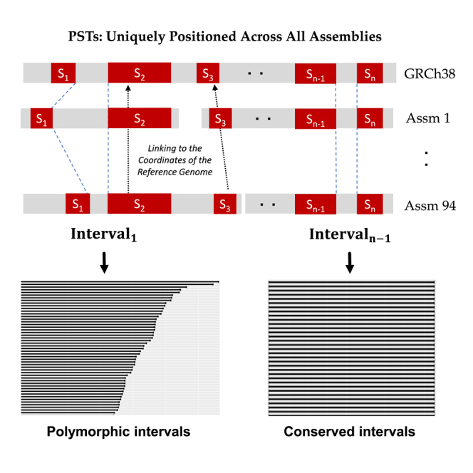
Based on the GRCh38 coordinates, we observed that 1.55 × ${10}^9$ (98.7%) of the identified 31-mers had consecutive positions on autosomes (Figure S2A). Similar trends were observed for both sex chromosomes. Consecutive overlapping 31-mers define longer segments of sequence that were present across all haploid assemblies—we refer to these extended sequences as PSTs (Figure 1A). The set of PSTs was distributed across all chromosomes (Figure 1B) and specific genome features including exonic, intronic, and intergenic regions (Figure 1C). As expected, centromeres and the acrocentric regions in the p arms of specific chromosomes had a lower density of PSTs—this was a result of their highly repetitive sequence structure. We confirmed that PSTs were present in all haploid genomes (see STAR Methods).

Figure 1.

Identification of pan-conserved segment tag in HPRC assemblies and their properties based on GRCh38 coordinates

(A) We define PST as when the set of consecutive unique sequence is present in all assemblies.

(B) The distribution of PSTs on GRCh38. The density of PSTs was calculated in 500 kb window; number of pan-conserved 31-mers/size of window.

(C) The distribution of PSTs across the different types of genomics regions on chr20. Annotate genomic regions with N’s as N regions.

(D) Change rate (%) in number of pan-conserved 31-mers in relation to number of included haploid assemblies.

Characteristics of the PSTs

The median length of an individual PST was 64 bp, with a range from 31 bp (from an individual 31-mer) up to a maximum size of 5.26 kilobase (kb) (Figure S2B). There were 24 PSTs from autosomes with lengths greater than 2.5 kb and mapped to genome coordinates in both GRCh38 and CHM13 (Table S2). The longest PST appeared on chromosome 5q31.3, where two genes (PURA and IGIP) with single exons are located. Thus, this same segment was the same among all assemblies. In addition, we confirmed that this 5q31.3 segment lacked any variants with a population frequency of 1% or higher according to the Genome Aggregation Database (gnomAD).¹² Interestingly, this chromosome 5 (chr5) PST contains PURA, which is considered the crucial gene for 5q31.3 microdeletion syndrome.¹³ This result may indicate that these PST genomic regions may have genes that have a functional requirement for conservation. Furthermore, the sequence alignment of this region among 30 different species of mammals showed that this segment was highly conserved across all primates, mice, and dogs.^14,15 Moreover, there were four additional PSTs that overlapped with loci associated with known disorders including Primrose syndrome, Wiedemann-Steiner syndrome, testicular germ cell cancer, and breast cancer with embryonic lethality (refer to Table S2 for further details).

Based on the coordinates of CHM13, we observed similar PST characteristics, which included (1) the density of pan-conserved 31-mer tags, (2) distance between tandem pan-conserved 31-mer tags, and (3) the length distributions of PSTs (Figure S3).

The sex chromosomes were evaluated for conserved regions. We identified PST conserved segments with lengths greater than 2.5 kb. ChrX had 22 PSTs, and chrY had 44 PSTs (Table S2). These sex chromosome PSTs came from 75 chrX haploids and 19 chrY haploids. This difference in number accounts for the relatively higher number of PSTs observed on chrX and the much larger number observed on chrY. ChrX had 22 PSTs, which is significantly higher compared with chr7 or chr8, both of which had two long PSTs per chromosome. Among the 22 PSTs on chrX, there 14 genes including POLA1, CNKSR2, ATP6AP1, ZIC3, and THOC2 (Table S2). The gnomAD variants with a population frequency of 1% were rarely reported in these long PSTs (Table S2). Citing some examples relevant to genetic diseases, we identified several long PSTs from chrX that overlapped with genetic disorders such as (1) CASK (calcium/calmodulin dependent serine protein kinase)-related intellectual disability, (2) Cockayne syndrome type B, and (3) X-linked intellectual disability-short stature-overweight syndrome (Table S2).

Number of PSTs remains stable despite increasing number of haploid assemblies

We investigated the relationship between the number of haploid assemblies and the number of PSTs. For this analysis, we compared the number of autosomal pan-conserved 31-mers and their PSTs identified from N haploid assemblies (briefly, PST(N)) with N+1 haploid assembly (PST(N+1)). The change rate was calculated as (PST(N+1) – PST(N))/PST(N). Examining GRCh38 alone, we identified 2.29 billion unique 31-mers. With the analysis of both GRCh38 and CHM13, we identified 2.20 billion pan-conserved 31-mers. This resulted in a change rate of −0.03512. When considering GRCh38, CHM13, and HG01891 maternal haploid assembly, we identified 2.16 billion PSTs, resulting in a change rate of −0.02425.

We then proceeded to identify pan-conserved 31-mers by sequentially including an increasing number of haploid assemblies from the pangenome. Finally, we identified 1.622 billion pan-conserved 31-mers among 95 assemblies without HG002 paternal assembly and 1.621 billion pan-conserved 31-mers among 96 assemblies, including HG002 paternal assembly. The resulting change rate was −0.00083. Overall, we observed a decrease in the change rate as the number of haploid assemblies included in the PST analysis increased (Figure 1D). In fact, the change rate remained at −0.0035 or closer to zero after including 59 or more haploid assemblies. This represents a plateau where the number of conserved sequences stabilizes. Based on these findings, we anticipate that the vast majority of PSTs in the current set will be present in any new haploid assembly.

Intervals between PST pairs among the pangenome assemblies

The interval length between cis-based tandem pairs of PSTs provided a way to determine the presence of SV among the individual haploid assemblies. By systematically examining all PST pairs, we determined the interval lengths among all haploid genomes and determined the differences in interval lengths compared with the reference. Variations in interval length for any given haploid genome are indicators of SVs (Figure 2A). A constant interval length across haploid genomes implies the absence of SVs, while a SV introduces changes in the interval length.

Figure 2.

Intervals between PSTs

(A) The three types of interval lengths relative to the interval length on GRCh38: (1) no arrangement: interval length on an assembly is identical to the length on GRCh38; (2) insertion: interval length on an assembly is larger than the length on GRCh38; and (3) deletion: interval length on an assembly is less than the length on GRCh38.

(B) Measuring length of intervals between adjacent pan-conserved sequence pair after sorting them by GRCh38 coordinates. A small number (<0.00001%) of tandem pairs of PSTs were on different contigs for a given haploid genome thanks to the high quality of HPRC assemblies (i.e., S₂ and S₃ in Assm1).

(C) The distribution of polymorphic intervals with Shannon diversity index of the divergent lengths across assemblies. S_i indicates the i^th PST, while Assm stands for assembly.

This evaluation involved the two steps (Figure 2B): (1) all PSTs were sorted for each chromosome based on the GRCh38 coordinates using a p- to q-arm orientation, and (2) we calculated the length of the interval sequence between any two tandem PST pairs within a given assembly contig. We conducted this process for all 94 HPRC haploid assemblies and constructed a data matrix where the columns represented a given haploid genome and the rows represented the lengths between consecutive PSTs (Figure S4). This matrix contained approximately 13.5 million rows with the interval lengths between tandem pairs of PSTs for a given haploid assembly (see "Interval lengths across all assemblies" in the key resources table). This matrix provided a rapid way to identify intervals with the same versus different lengths across 94 assemblies. Similarly, we produced a matrix comprising 629,000 rows for 75 haploids with chrX, as well as another matrix with 94,000 rows for 19 haploids with chrY.

PSTs have limits when mapped to the contigs with either the p and q telomeres. The pangenome has not released complete chromosome assemblies, meaning a T2T chromosome assembly. The breaks between contigs prevented some tandem segments from being compared (Figure 2B). This represented only a small fraction of the HPRC assemblies.

Conserved intervals across the pangenome

Among the 13.5 million intervals from autosomes, we identified approximately 11.3 million (83.6%) where the sequence lengths were identical among all 94 assemblies. The uniform interval length implied that the intervening sequences were the same, albeit there could be variants such as SNPs, which do not change the number of bp. These “conserved intervals” indicate the segments of the pangenome with a high degree of structural conservation. We used the Matched Annotation from NCBI and EMBL-EBI (MANE) resource to determine coding regions for each conserved interval.¹⁶ Approximately 51 Mb (67.5%) of exonic regions and 905 Mb (73%) of genic regions including introns overlapped with the conserved intervals. 520 conserved regions were longer than 10 kb (Table S3). The longest region (chr13:102,729,323–102,751,307) spanned 22 kb across the gene CCDC168. More than half of the conserved regions occurred outside of genic regions, and the longest one spanned 18 kb at chr2:63,078,147–63,096,212, which had no reported protein-encoding gene.¹⁵

We observed a similar extent of conservation among the sex chromosomes, with 86.4% of all intervals on chrX and 94.5% of all intervals on chrY being conserved intervals. On chrX, we identified 121 conserved intervals with a length greater than 10 kb, while on chrY, we found 290 such intervals (Table S3). As we mentioned previously, the large number of long conserved intervals on chrY may be attributable to the size of the haploid set, consisting of only 19 paternal haploids from males. Of the 121 long conserved intervals on chrX, 47 intervals overlapped with genic regions, with 28 of them overlapping with exonic regions. The longest conserved interval (∼20 kb) was located at chrX:104,672,152–104,692,096, which was located between the introns of two genes, IL1RAPL2 and TEX13A.

Divergent interval lengths point to loci with polymorphic SVs

Changes in the PST interval lengths are indicators of SVs. We identified 60,763 (0.45%) autosomal intervals that had divergent lengths of 50 bp or greater compared with the GRCh38 for at least one haploid assembly among all assemblies (Table S4). The median divergent lengths within the size range of 100 bp to 1 kb represented the most frequent category, constituting 47.2% of polymorphic intervals (Table S5). As we show per our results, these divergent lengths defined the location of structural polymorphisms that were present throughout the pangenome. Overall, we observed that the number of longer divergent lengths (indicating insertion) is larger than shorter divergent lengths (indicating deletion) (Table S6). For interval lengths ranging up to 1 kb, we observed minimal divergence in the length, meaning that the same size intervals were observed across all haploid genomes. As expected, longer interval lengths among the pangenome assemblies diverged more frequently from GRCh38. Interestingly, intervals in the size range of the 1 to 10 kb bracket or the 10–100 Mb brackets were generally shorter than what was calculated from GRCh38.

We observed that 46,516 polymorphic intervals overlapped with repeats per a comparison with the RepeatMasker annotation (4.0.6). There were 12,906 intervals located within repeat sequences and motifs. For the size range up to 100 kb, the LINE/L1s had the most frequent overlap. For the size range of 100 kb to 1 Mb and 1–10 Mb, SINE/Alus and LTR/ERVL-MaLRs had the most frequent overlap. Interestingly, we observed different trends for shorter divergent lengths: simple repeat for 50–100 bp, SINE/Alu for 100–500 bp, and LINE/L1 for 500–1,000 bp. Additional categories are listed in Table S7.

61 polymorphic intervals were located within the coding exon regions and thereby changed the lengths of the coding sequences in 39 genes, such as MUC6, MYH8, and ATG9B. The vast majority (>95%) of these different interval lengths were related to in-frame variants (Table S8). Citing an example, all 94 assemblies had different lengths for exon 31 of MUC6 compared with GRCh38.

Next, we characterized the polymorphic intervals based on the frequency of the divergent lengths among the haploid genomes: (1) singletons, which are present in only one haploid assembly, (2) low-frequency intervals (1%–5%), and (3) high-frequency intervals (>5%) (Table S5). Interestingly, singletons were very frequent (28.7%). There was one class of singletons that were directly related to the GRCh38. We identified 253 intervals that had identical lengths among all 94 assemblies but differed only for GRCh38—this category was made of up indicators of a reference limitation. Citing an example, all 94 assemblies had an additional 252 bp in the last exon of ZNF676 on chr19—only the GRCh38 reference lacked this feature. The remaining singletons were indicators of potential SVs that were unique to an individual haploid genome. In general, the number of total polymorphic intervals and singletons per assembly was higher among the AFR genome compared with other populations (Table S9). This observation is consistent with what has been reported by other studies.¹⁷

We measured the extent of variability for these polymorphic intervals by (1) the Shannon-Wiener diversity index and (2) the inter-quartile range (IQR). The diversity index provides a quantitative metric regarding the extent of different interval lengths, while the IQR value provided information on the magnitude of length variation (STAR Methods). The median of the Shannon-Wiener diversity index for intervals was 0.42. The values ranged from 0 (when all 94 assemblies have an interval length) to 6.56 (when all 94 assemblies have different lengths) (Figure 2C). Notably, three intervals had different lengths for all 93 individual assemblies. The first one was located at chr11:11,246,448–112,472,12 with median different lengths of 4.4 kb overlapped with long terminal repeats (LTRs) and simple repeats. The second one occurred at chr13:111,793,323–111,843,451 with median different lengths of 94 kb that did not overlap with any genes or repeats. Within the interval of chr15:34,278,120–34,586,890 with median different lengths of 5.2 kb, there were several genes including SLC12A6 and NOP1 and repeats such as SINE, LINE, and simple repeats. As an example, we show all divergent interval lengths for 94 assemblies on chr18 in Figure 3A. The other chromosomes are shown in Figure S5. We highlighted three examples: (1) the most polymorphic interval on chr18 (Figure 3B), (2) an interval with the largest divergent length (Figure 3C), and (3) an interval length with a high frequency (Figure 3D).

Figure 3.

Polymorphic intervals on chr18

(A) The locations of polymorphic intervals across chr18. Blue dots indicate the median of interval lengths, while gray dots indicate the interval length of an assembly.

(B) A highly polymorphic interval, with a size of 4.67 kb as per GRCh38, exhibited 92 different lengths, resulting in a diversity index of 6.51.

(C) Long polymorphic interval had the highest IQR of divergent length relative to the reference interval size of 47 kb.

(D) A biallelic polymorphic interval with high frequency (0.457) has a binomial distribution of different lengths (658 bp deletion for 43 assemblies; no changes for 51 assemblies). The entire region of this interval is annotated as LINE by RepeatMasker.

(E) Population-specific intervals with divergent lengths only for AFR and AMR. The interval at chr16:82,043,368–82,043,731 had a deletion of 322 bp on intron 1 of SD17B2. This deletion was present exclusively among the 25 AFR assemblies, where 12 of them were homozygous for 6 individuals.

Finally, we identified some of the divergent intervals associated with specific biogeographic populations (Table S10). We found 381 divergent intervals with polymorphic lengths present in only a single superpopulation (Figure 3E). We cite examples in which the divergent interval lengths were present in 10 or more assemblies: 376 were specific to the AFR superpopulation, and 5 were specific to the AMR superpopulation. We also observed 59 intervals with the reverse attribute. For example, the chr12:102,848,406–102,848,539 interval had a 70 bp deletion among 59 assemblies, but this deletion was not present among all 10 EAS assemblies.

For the sex chromosomes, we identified 2,411 (0.35%) divergent intervals on chrX and 167 (0.17%) on chrY (Table S11). The characteristics of the divergent intervals on chrX were similar to those on autosomes. However, we observed finding about chrY, where 33 out of 167 (20.4%) intervals had the same length in the 19 HPRC assemblies but differed from the length in GRCh38.

Enrichment analysis for genes in long PSTs and conserved and polymorphic intervals

Using the program FUMA,¹⁸ we conducted a Gene Ontology (GO) enrichment analysis for genes in conserved regions with the following properties: (1) long PSTs with sizes >2.5 kb, (2) conserved intervals with sizes >10 kb, or (3) polymorphic intervals. For long PSTs, we identified 40 genes that were associated with hippocampus tail volume. For long conserved intervals, we identified 349 genes significantly enriched for several functions such as obesity-related traits and general risk tolerance (multitrait analysis of GWAS, MTAG) (Figure S6). In addition, our analysis revealed 448 genes that had a significant enrichment related to keratin filament.

Polymorphic intervals compared with reported SVs

We examined whether the polymorphic intervals were overlapping with SVs reported from 1000 Genomes Project (1KGP).¹⁹ We observed that 15,869 (92.1%) out of 17,224 simple SVs from 1KGP overlapped with one of polymorphic intervals (Table 1). We excluded insertions from analysis since this class of SVs are the most challenging to accurately call and are still vastly underrepresented in gold-standard call sets.^20,21 The high overlapping indicates that the analysis of the pangenome provided a way to identify regions of the genome that contain SV polymorphisms in the population.

Table 1.

The number of 1000 Genome Project SVs overlapping with the polymorphic intervals

Interval lengths difference	DEL (12659)	DUP (4343)	INV (222)
<100 bp	250	859	52
100 bp to 1 kb	6,063	1,247	104
1–10 kb	3,120	448	28
10–100 kb	1,060	435	14
100 kb to 1 Mb	872	591	6
1–10 Mb	272	226	5
10–100 Mb	382	109	9
Total (%)	11,909 (93.8)	3,776 (86.2)	184 (82.3)

We compared the polymorphic intervals with 17,224 simple SVs with >1% frequency from 1KGP. Simple SVs include deletion (DEL), duplication (DUP), and inversion (INV). The polymorphic intervals were grouped by their median of different lengths. The numbers in bold indicate the most frequent length difference in each SV type.

Benchmarking divergent intervals as indicators of structural variants

To demonstrate that the polymorphic intervals were indicators of SVs, we examined the HG002 genome for the presence of deletions, insertions, and other SVs. HG002 is part of the pangenome, and this individual has also undergone an extensive genomic analysis by the Genome in a Bottle (GIAB) Consortium. Per the GIAB analysis, HG002 had 250 SVs located in the vicinity of medically relevant genes.²² We compared 220 SVs that had a size of 50 bp or greater with our polymorphic intervals. Remarkably, all 220 SVs were located within the polymorphic intervals found in the pangenome (Table S12). The size of most SVs (74.5%) had the same lengths as those described by divergent interval lengths. Another subset of SVs (11%) had minor differences in lengths by less than 15 bp. For a small subset of the SVs, the reported size from the GIAB benchmark did not match our divergent interval length. There were 31 intervals that had a median length of 100 kb—these long intervals contained multiple SV structures that led to a difference.

Visualizing the structure of SVs using constituent sequences from the pangenome

Providing an example, we are using the constituent 31-mers of SVs to visualize the structure of different classes of SVs including insertions, deletions, duplications, inversions, and more complex rearrangements. This process involved using a simple dot matrix plot with the two axes representing the GRCh38 and the specific haploid assembly. We plotted the position of the 31-mers that spanned the divergent interval (Figure 4A). We showed six different SV classes occurring in these divergent intervals (Figures 4B–4G). As expected, longer intervals indicated either insertions or tandem duplication, while shorter intervals indicated either a deletion or a complex SV. Furthermore, we were able to characterize the structure of a highly complex SV identified in CHM13. This complex SV involved nine different structural changes that included multiple insertions, deletions, and inversions (Figure 5).

Figure 4.

The SV plots using 31-mers from polymorphic intervals

(A) The scheme of plotting 31-mers from both reference and query assemblies to depict SVs.

(B–G) Examples of different types of SVs are shown: (B) insertion, (C) deletion, (D) tandem duplication, (E) multiple duplications, (F) inversion, and (G) complex SVs.

Figure 5.

Anatomy of complex SV

We demonstrate that an SV plot displays the various components within a complex SV.

Examples of how PSTs identify SVs

We demonstrate the application of PSTs for identifying SVs in two basic steps. First, we identify the flanking PSTs that are closest to the start (up PTS) and end positions (down PST) of the regions of interest. This analysis uses the bedtools intersect function. Second, we measure the interval lengths between selected PST pairs and compare the lengths to GRCh38. This step determines any changes in lengths. For example, with this process, we identified an insertion of 108 bp at exon 12 of IGFN1 on the HG002 maternal haploid. In addition, we observed that the length of variable number tandem repeat (VNTR) on chr1:106,430,881–106,431,449 (568 bp) on GRCh38 are changed to 798 bp on both the HG002 maternal and paternal haploids. We provided all scripts to identify flanking PSTs and measure the intervals used in these examples at our GitHub: https://github.com/compbio/pan-conserved_segments.

Discussion

The HPRC has released its first draft of human pangenome derived from 94 haploid assemblies of 47 individuals with diverse genetic backgrounds.⁷ The pangenome’s new features provide increased representation of genomic and geographic diversity and haplotype structure. With its improved sequence assembly, it addresses the limitations of the current linear reference genome, GRCh38. To promote the adoption of the pangenome reference, it is critical to compare these assemblies with the reference genomes. Thus, there is a need for new approaches to enable the research community to utilize the pangenome reference in sequencing analysis.

As we have described, this k-mer indexing approach enables one to conduct multigenome comparisons efficiently and in a highly scalable fashion. For identifying conserved versus divergent sequence features, this approach has several advantages over conventional sequence alignment, particularly in a multiple genome comparison. First, PSTs are independent of any individual genome’s coordinates—this allows one to use the coordinates for a given assembly or any other reference such as GRCh38. Demonstrating this feature, we have provided all our results in CHM13 coordinates as supplemental files in addition to ones based on GRCh38. Another advantage is that it can be used on incomplete assemblies and long-read sequences. This feature also allows direct comparison among different genomes. For instance, we observed an average of 14,522 deviated lengths relative to GRCh38 per haploid assembly, while we observed an average of 11,936 divergent interval lengths between maternal and paternal haploids from an individual. Divergent interval lengths based on PSTs point to potential structural variants such as deletions. As noted in our results, these divergent lengths revealed a set of genome loci that are highly polymorphic. Finally, the long stretch of PSTs may indicate ultra-conserved sequences, which could indicate syntenic regions when they are found across multiple species. For future studies, we will index the reference genomes from multiple species including primates and identify PSTs across different species.

Beyond the identification of polymorphic loci in the genome, this approach and the related resource can be used to rapidly visualize SV structures. Juxtaposition of k-mers involving SVs from two assemblies can reveal general structure SVs including complex ones (Figures 4 and 5). Specifically, one can use other classes of 31-mers without some of the stringent criteria metrics and apply this expanded set for identifying rearrangement features. For example, these 31-mers with looser sequence characteristics can distinguish tandem duplications with insertions. PSTs with their unique segments also provide an accessible way of visualizing complex SVs. For example, S₁S’₄S’₃S’₂S₅ describes the inversion of S₂S₃S₄ and S₁S₂S₃S₄S₁S₅ describes interspersed duplication of S₁ when a reference looks like S₁S₂S₃S₄S₅, where S₁, S₂, S₃, S_4, and S₅ represent PST/unique segments. Negative interval lengths may pinpoint the rearranged PST due to SVs including inversion. For future studies, we will develop computational tools to determine the breakpoints of SVs with their k-mer plots and PSTs. Thus, we propose a computational framework for SV identification in two steps: (1) identifying the presence of SVs using PSTs and (2) characterizing them using k-mer plots.

As a resource for the research community, we provide our interval matrix of 94 HPRC assemblies against GRCh38/CHM13 in a BED format. This file is readily accessible and is formatted such that it can be used across a variety of different applications. Other researchers can take advantage of this matrix of pangenome conserved/divergent sequences to see which regions contain their variants of interest. Furthermore, our method using PSTs to split de novo haploid assemblies in the same manner enables systematic characterization of genomic conservation and divergence.

The HPRC will be expanding the pangenome reference to include more haploid assemblies.⁶ This approach is readily scalable across hundreds of genomes. Thus, we can readily update this resource for the final release. In summary, the comparison of available haploid assemblies relative to the reference genomes in a timely manner will enable using the pangenome resource and holds the potential to further accelerate new genetic discoveries.

Limitations of the study

Divergent interval lengths suggest the presence of potential SVs—additional characterization is needed to determine the exact SV structures. When multiple SVs occur within an interval, the differences in interval length are simply the sum of the individual different lengths. As an example, an interval with one insertion of 1 kb and a deletion of 750 bp results in a net gain of 250 bp. In addition, certain segments of the genome do not have PSTs. For example, we identified 38 regions on autosomes of GRCh38 longer than 1 Mb without any PSTs (see Table S13). Finally, SVs that do not alter the length of sequences, such as inversions, cannot be detected through the examination of interval lengths.

Consortia

The members of the Human Pangenome Reference Consortium are Wen-Wei Liao, Mobin Asri, Jana Ebler, Daniel Doerr, Marina Haukness, Glenn Hickey, Shuangjia Lu, Julian K. Lucas, Jean Monlong, Haley J. Abel, Silvia Buonaiuto, Xian H. Chang, Haoyu Cheng, Justin Chu, Vincenza Colonna, Jordan M. Eizenga, Xiaowen Feng, Christian Fischer, Robert S. Fulton, Shilpa Garg, Cristian Groza, Andrea Guarracino, William T. Harvey, Simon Heumos, Kerstin Howe, Miten Jain, Tsung-Yu Lu, Charles Markello, Fergal J. Martin, Matthew W. Mitchell, Katherine M. Munson, Moses Njagi Mwaniki, Adam M. Novak, Hugh E. Olsen, Trevor Pesout, David Porubsky, Pjotr Prins, Jonas A. Sibbesen, Chad Tomlinson, Flavia Villani, Mitchell R. Vollger, Lucinda L. Antonacci-Fulton, Gunjan Baid, Carl A. Baker, Anastasiya Belyaeva, Konstantinos Billis, Andrew Carroll, Pi-Chuan Chang, Sarah Cody, Daniel E. Cook, Omar E. Cornejo, Mark Diekhans, Peter Ebert, Susan Fairley, Olivier Fedrigo, Adam L. Felsenfeld, Giulio Formenti, Adam Frankish, Yan Gao, Carlos Garcia Giron, Richard E. Green, Leanne Haggerty, Kendra Hoekzema, Thibaut Hourlier, Hanlee P. Ji, Alexey Kolesnikov, Jan O. Korbel, Jennifer Kordosky, HoJoon Lee, Alexandra P. Lewis, Hugo Magalhães, Santiago Marco-Sola, Pierre Marijon, Jennifer McDaniel, Jacquelyn Mountcastle, Maria Nattestad, Nathan D. Olson, Daniela Puiu, Allison A. Regier, Arang Rhie, Samuel Sacco, Ashley D. Sanders, Valerie A. Schneider, Baergen I. Schultz, Kishwar Shafin, Jouni Sirén, Michael W. Smith, Heidi J. Sofia, Ahmad N. Abou Tayoun, Françoise Thibaud-Nissen, Francesca Floriana Tricomi, Justin Wagner, Jonathan M.D. Wood, Aleksey V. Zimin, Alice B. Popejoy, Guillaume Bourque, Mark J.P. Chaisson, Paul Flicek, Adam M. Phillippy, Justin M. Zook, Evan E. Eichler, David Haussler, Erich D. Jarvis, Karen H. Miga, Ting Wang, Erik Garrison, Tobias Marschall, Ira Hall, Heng Li, and Benedict Paten.

STAR★Methods

Key resources table

REAGENT or RESOURCE	SOURCE	IDENTIFIER
Deposited data
GCA_000001405.15_GRCh38_no_alt_analysis_set.fna	National Center for Biotechnology Information (NCBI)	https://ftp.ncbi.nlm.nih.gov/genomes/all/GCA/000/001/405/GCA_000001405.15_GRCh38/seqs_for_alignment_pipelines.ucsc_ids/
chm13.draft_v1.1.fasta	National Center for Biotechnology Information (NCBI)	https://www.ncbi.nlm.nih.gov/assembly/GCA_009914755.3/
All HPRC haploid assemblies	The Human Pangenome Reference Consortium (HPRC)	https://github.com/human-pangenomics/HPP_Year1_Assemblies
CMRG benchmark containing medically relevant SVs	Genome in a Bottle (GIAB)	https://ftp-trace.ncbi.nlm.nih.gov/ReferenceSamples/giab/release/AshkenazimTrio/HG002_NA24385_son/CMRG_v1.00/GRCh38/StructuralVariant/
1KGP_3202.gatksv_svtools_novelins.freeze_V3.wAF.vcf	1000 Genome Project	http://ftp.1000genomes.ebi.ac.uk/vol1/ftp/data_collections/1000G_2504_high_coverage/working/20210124.SV_Illumina_Integration/
The sequences and coordinates of pan-conserved sequences tag (PSTs)	This manuscript	https://dna-discovery.stanford.edu/publicmaterial/datasets/pangenome/
Intervals lengths across all assemblies	This manuscript	https://dna-discovery.stanford.edu/publicmaterial/datasets/pangenome/
Software and algorithms
R	R 4.1	N/A
Python	Python 3.8	N/A
Analysis code for this paper	This paper	https://doi.org/10.5281/zenodo.8088496
Functional Mapping and Annotation (FUMA, 1.5.3)	https://doi.org/10.1038/s41467-017-01261-5	RRID:SCR_017521
The web version of KmerKeys	https://doi.org/10.1093/nar/gkac266	https://kmerkeys.dgi-stanford.org/

Resource availability

Lead contact

Further information and requests for resources and reagents should be directed to and will be fulfilled by the lead contact, Hanlee Ji (genomics_ji@stanford.edu).

Materials availability

This study did not generate new unique reagents.

Method details

The sequences of human genome assemblies

In this study, we analyzed a total of 47 individuals with 94 haploid human genome assemblies in addition to two references from the following sources; 1) GRCh38, 2) CHM13, and 3) 94 HPRC haploid assemblies. We obtained the following assemblies from the National Center for Biotechnology Information (NCBI). From GenBank, we downloaded the 94 haploid assemblies from 47 individuals, which generated by HPRC (Year 1 freeze GenBank). The accession number of assemblies are listed in Table S1. The HPRC samples underwent whole genome sequencing that included long sequence reads (Pacific Biosciences, Oxford Nanopore), optical mapping (Bionano) and high coverage short read sequencing. The consortium developed a bioinformatic pipeline with multiple quality control metrics. The production process included evaluating the completeness, contiguity, base-level quality, and phasing accuracy of each haploid assembly.

The structural variant data

For benchmarking HG002, we downloaded GIAB CMRG benchmark containing medically relevant SVs. In addition, we downloaded 17,224 SVs (deletions, duplications, and inversions) called from high-coverage whole-genome sequencing of the expanded 1000 Genomes Project cohort.¹⁹ We overlapped them with the polymorphic intervals using bedtools (v2.27): bedtools intersect -wa -wb -b $polymorphic_intervals.bed -a $sv_1kgp.bed. In instances where an SV overlaps with multiple polymorphic intervals, we selected polymorphic intervals with the maximum base-pair overlap.

K-mer indexing of assemblies

To characterize these assemblies, we indexed them using our k-mer-based indexing strategy.⁹ A given assembly are indexed in two steps (Figure S7A).

• Step 1:

  retrieve the sequence of k-mers with sliding window with 1 bp increments.

• Step 2:

  Associate the k-mers with genomics positions and their frequencies.

Citing an example, for the first substring of length 3 at position 1 is AAT and second substring at position 2 is ATA. We repeat this process from first position to (n-k+1)^th position where n = the length of assembly and k is the length of substring. We counted canonical k-mers, where k-mers are identical to their reverse complement, and selected a sequence based on lexicographical order. For instance, CGA is selected for S₆ instead of TCG. The frequency of AAT is 2 since AAT appears at position 1 and position 4 while the frequency of ATA is 1.

We repeat this process with all assemblies and build a large index for all assemblies of interest (Figure S7B). This index enables us to retrieve the information through sequences from indexed assemblies such as the list of assemblies with query sequences and their locations in each assembly.

Defining the properties of k-mers in a haploid genome assembly

For this study, we defined three categories of k-mer metrics derived from a given haploid genome assembly: (1) total set of k-mers, (2) the non-duplicated, distinct k-mers, (3) unique k-mers (Figure S7A). Given an assembly A of length L, the first metric describes the total number of k-mers of length k that are present in a given genome assembly (A). Thus, this is a count for every sequence substring. We denote the sequence substring of length k at position i in A as $S_i$.

$$\mathbf{T}\mathbf{o}\mathbf{t}\mathbf{a}\mathbf{l}\mathbf{s}\mathbf{e}\mathbf{t}\mathbf{o}\mathbf{f}\mathbf{k}-\mathbf{m}\mathbf{e}\mathbf{r}\mathbf{s}=\left\{S_1,S_2\dots ,S_{L-k+1}\right\}$$

The second metric involves identify and counting all of the different sequences from the total number of k-mers which are not duplicated (distinct). We denote i^th k-mers as $k_i$ after sorting all substrings in lexicographic order.

$$\mathbf{D}\mathbf{i}\mathbf{s}\mathbf{t}\mathbf{i}\mathbf{n}\mathbf{c}\mathbf{t}\left(\mathbf{o}\mathbf{r}\mathbf{n}\mathbf{o}\mathbf{n}-\mathbf{d}\mathbf{u}\mathbf{p}\mathbf{l}\mathbf{i}\mathbf{c}\mathbf{a}\mathbf{t}\mathbf{e}\mathbf{d}\right)\mathbf{k}-\mathbf{m}\mathbf{e}\mathbf{r}\mathbf{s}\mathrm{w}\mathrm{i}\mathrm{t}\mathrm{h}\mathrm{t}\mathrm{h}\mathrm{e}\mathrm{i}\mathrm{r}\mathrm{c}\mathrm{o}\mathrm{u}\mathrm{n}\mathrm{t}\mathrm{s}=\left\{k_1:f\left(k_1\right),k_2:f\left(k_2\right),\dots ,k_n:f\left(k_n\right)\right\}$$

where ($f\left(k_i\right)$ is the count of observed $k_i$ in A.

The next k-mer metrics involves the sequence substring of length k which are present only once (unique) from the total set of k-mers for a given haploid assembly. Therefore, unique k-mers in A are all $k_i$ with ($f\left(k_i\right)$ = 1

$${\mathbf{U}\mathbf{n}\mathbf{i}\mathbf{q}\mathbf{u}\mathbf{e}\mathbf{k}-\mathbf{m}\mathbf{e}\mathbf{r}\mathbf{s};Uniq}_A=\left\{allk:f\left(k_i\right)=1\right\}$$

The definition of “pan-conserved k-mers tag”

From multiple haploid assemblies from different individuals, we define a highly conserved subset of k-mers that have the following properties: (1) are non-duplicated and thus distinct per a given haploid genome; (2) found only once per a given haploid genome and thus are unique; (3) are observed across all of the assemblies with the same properties. For the last point, this k-mer subset represents an intersection across all assemblies. This k-mers from this intersection are conserved across all individual genomes that were included in this total set of assemblies.

$$\mathrm{I}\mathrm{n}\forall ,\mathrm{p}\mathrm{a}\mathrm{n}-\mathrm{c}\mathrm{o}\mathrm{n}\mathrm{s}\mathrm{e}\mathrm{r}\mathrm{v}\mathrm{e}\mathrm{d}\mathrm{k}-\mathrm{m}\mathrm{e}\mathrm{r}\mathrm{s}\mathrm{t}\mathrm{a}\mathrm{g}={\cap }_{\mathrm{i}=1}^N\left({Uniq}_{\mathrm{A}\mathrm{i}}\right)where\forall =\left\{A_1,A_2,\dots ,A_N\right\}$$

Namely, the k-mers which are not-duplicated, unique per a given haploid assembly and have these same properties across all individuals in a collection of genomes. To facilitate referring to this set of k-mers, we will use an acronym that describes these properties: pan-conserved segment tag or PSTs. This definition has advantages in that it can be adjusted for new haploid genome assemblies as they become available. For chrX and chrY, we only considered maternal haploids from males and both haploids from females for pan-conserved k-mers tag on chrX. Likewise, only paternal haploids from males were examined for pan-conserved k-mers tag on chrY.

We will consider an example from Assembly 1. The sequence AATAATCGA has total 7 substrings of length 3; {$S_1$, $S_2$.. , $S_7$} and 4 distinct 3-mers since the sequences of $S_1$ and $S_4$ as well as $S_6$ and $S_7$ are identical. There are 3 unique 3-mers out of 5 distinct 3-mers, ${Uniq}_{\mathrm{A}1}$ = {ATA, ATC, TAA}. We repeated same process with Assembly 2 and 3 to identify ${Uniq}_{\mathrm{A}2}$ = {ATC, CAA, CAC, GAC} and ${Uniq}_{\mathrm{A}3}$ = {AAT, ATC, CGA, GAA}. We identify pan-conserved 3-mers tag by ${Uniq}_{\mathrm{A}1}$ ∩ ${Uniq}_{\mathrm{A}2}$ ∩ ${Uniq}_{\mathrm{A}3}$ = {ATC}. Among 3 assemblies, ATC is only pan-conserved tag sequence since it is unique in assembly 1, 2, and 3 respectively. AAT is not pan-conserved 3-mers tag since ATT ∉ ${Uniq}_{\mathrm{A}1}$. All other unique 3-mers are not present in all assemblies. For instance, CAA is not pan-conserved 3-mer tag because CAA ∈ ${Uniq}_{\mathrm{A}2}$, but CAA ∉ ${Uniq}_{\mathrm{A}1}$ and CAA ∉ ${Uniq}_{\mathrm{A}3}$.

The pan-conserved segment tags (PSTs) in all assemblies

The total number of PSTs used in this study was ∼13.48 × ${10}^6$ and checked if the sequences of them were maintained in same way across all assemblies. To confirm the preservation of PSTs across all assemblies, we evaluated the lengths between following number of non-overlapping 31-mers within pan-conserved segments: ceil(L/31) where ceil is the ceiling function and L is the length of pan-conserved segments. For instance, we checked 3 of non-overlapping constituent 31-mers of a PST with size of 100 bp. We found out that the lengths of 237 PSTs were different in several assemblies (Table S14). This happened when one of constituent pan-conserved 31-mer tag were accidently identical to a 31-mer from other location due to SNP.

The matrix of interval lengths between the PSTs across 94 assemblies

The genomic arrangements were measured by the length of intervals between adjacent PST. Possible genomic rearrangements in a given assembly can be estimated based on the difference in the interval length (deviated lengths) as follows.

• •Deletion: $D_i^{ref}>D_i^N$ > 0
• •Insertion: 0 < $D_i^{ref}$ < $D_i^N$

Calculation of all interval lengths involves the following steps: First, we sorted PST by their coordinates based on a reference, which is GRCh38 in this study. Second, we retrieve the location of PST on contigs from an assembly. Third, we measured the lengths between adjacent PST, $S_i$ and $S_{i+1}$,for i = 1 to n-1 for an assembly. The lengths between $S_i$ and $S_{i+1}$ is measured by their starting positions. The distance cannot be measured when $S_i$ and $S_{i+1}$ are on different contigs.

Since all contigs from an assembly were not in the same orientation, we determined the orientation of contigs based on the majority of signs of length. For instance, if there are more minus lengths than positive ones, we switched all signs of lengths.

Measuring the variability of interval lengths between adjacent PSTs across 94 assemblies

We identified PSTs by combining consecutive pan-conserved 31-mers tag into a segment. The n^th interval was defined from last 31-mers in n^th PST and first 31-mers in n+1^th PST. The PST with less than 50 pan-conserved 31-mers tag were represented only by their first pan-conserved 31-mers tag. Each interval has the lengths for 94 HPRC assemblies. The extent of variability for polymorphic-intervals was measured by (1) Shannon-Wiener diversity index and (2) inter-quartile range (IQR). First, we used a Python library called “scikit-bio”, which defines Shannon-Wiener diversity index as $-{\sum }_{i=1}^s\left(p_i{\log }_2{p}_i\right)$ where s is the number of different distinct lengths and $p_i$ is the proportion of the lengths of i. The Shannon-Wiener diversity shows how many different lengths are in an interval across 94 HPRC assemblies. Second, the inter-quartile range is calculated by Python NumPy library as follows: IQR = Q3 – Q1 where Q3 is 3^rd quartile value and Q1 is 1^st quartile value. The IQR value provides information on the magnitude of deviated lengths.

Published: August 2, 2023

Data and code availability

• •This paper analyzes existing, publicly available data. These accession numbers for the datasets are listed in the key resources table. New datasets generated from our studies were deposited in https://dna-discovery.stanford.edu/publicmaterial/datasets/pangenome and they are publicly available as of the data of publication.
• •All original code has been deposited at GitHub (https://github.com/compbio/pan-conserved_segments) as well as Zenodo and is publicly available as of the date of publication. DOIs are listed in the key resources table.
• •Any additional information required to reanalyze the data reported in this paper is available from the lead contact upon request.

References

- 1.Sherman R.M., Salzberg S.L. Pan-genomics in the human genome era. Nat. Rev. Genet. 2020;21:243–254. doi: 10.1038/s41576-020-0210-7. [DOI] [PMC free article] [PubMed] [Google Scholar]
- 2.Hurgobin B., Edwards D. SNP discovery using a Pangenome: has the single reference approach become obsolete? Biology. 2017;6:21. doi: 10.3390/biology6010021. [DOI] [PMC free article] [PubMed] [Google Scholar]
- 3.Miga K.H., Wang T. The need for a human pangenome reference sequence. Annu. Rev. Genomics Hum. Genet. 2021;22:81–102. doi: 10.1146/annurev-genom-120120-081921. [DOI] [PMC free article] [PubMed] [Google Scholar]
- 4.Zhou B., Arthur J.G., Guo H., Hughes C.R., Kim T., Huang Y., Pattni R., Lee H., Ji H.P., Song G., et al. Automatic detection of complex structural genome variation across world populations. bioRxiv. 2023 doi: 10.1101/200170. Preprint at. [DOI] [Google Scholar]
- 5.Nurk S., Koren S., Rhie A., Rautiainen M., Bzikadze A.V., Mikheenko A., Vollger M.R., Altemose N., Uralsky L., Gershman A., et al. The complete sequence of a human genome. Science. 2022;376:44–53. doi: 10.1126/science.abj6987. [DOI] [PMC free article] [PubMed] [Google Scholar]
- 6.Wang T., Antonacci-Fulton L., Howe K., Lawson H.A., Lucas J.K., Phillippy A.M., Popejoy A.B., Asri M., Carson C., Chaisson M.J.P., et al. The human pangenome project: a global resource to map genomic diversity. Nature. 2022;604:437–446. doi: 10.1038/s41586-022-04601-8. [DOI] [PMC free article] [PubMed] [Google Scholar]
- 7.Liao W.-W., Asri M., Ebler J., Doerr D., Haukness M., Hickey G., Lu S., Lucas J.K., Monlong J., Abel H.J., et al. A draft human pangenome reference. bioRxiv. 2022 doi: 10.1101/2022.07.09.499321. Preprint at. [DOI] [PMC free article] [PubMed] [Google Scholar]
- 8.Kille B., Balaji A., Sedlazeck F.J., Nute M., Treangen T.J. Multiple genome alignment in the telomere-to-telomere assembly era. Genome Biol. 2022;23:182. doi: 10.1186/s13059-022-02735-6. [DOI] [PMC free article] [PubMed] [Google Scholar]
- 9.Pavlichin D.S., Lee H., Greer S.U., Grimes S.M., Weissman T., Ji H.P. KmerKeys: a web resource for searching indexed genome assemblies and variants. Nucleic Acids Res. 2022;50:W448–W453. doi: 10.1093/nar/gkac266. [DOI] [PMC free article] [PubMed] [Google Scholar]
- 10.Lau B.T., Pavlichin D., Hooker A.C., Almeda A., Shin G., Chen J., Sahoo M.K., Huang C.H., Pinsky B.A., Lee H.J., Ji H.P. Profiling SARS-CoV-2 mutation fingerprints that range from the viral pangenome to individual infection quasispecies. Genome Med. 2021;13:62. doi: 10.1186/s13073-021-00882-2. [DOI] [PMC free article] [PubMed] [Google Scholar]
- 11.Lee H., Shuaibi A., Bell J.M., Pavlichin D.S., Ji H.P. Unique k-mer sequences for validating cancer-related substitution, insertion and deletion mutations. NAR Cancer. 2020;2:zcaa034. doi: 10.1093/narcan/zcaa034. [DOI] [PMC free article] [PubMed] [Google Scholar]
- 12.Karczewski K.J., Francioli L.C., Tiao G., Cummings B.B., Alföldi J., Wang Q., Collins R.L., Laricchia K.M., Ganna A., Birnbaum D.P., et al. The mutational constraint spectrum quantified from variation in 141,456 humans. Nature. 2020;581:434–443. doi: 10.1038/s41586-020-2308-7. [DOI] [PMC free article] [PubMed] [Google Scholar]
- 13.Bonaglia M.C., Zanotta N., Giorda R., D'Angelo G., Zucca C. Long-term follow-up of a patient with 5q31.3 microdeletion syndrome and the smallest de novo 5q31.2q31.3 deletion involving PURA. Mol. Cytogenet. 2015;8:89. doi: 10.1186/s13039-015-0193-9. [DOI] [PMC free article] [PubMed] [Google Scholar]
- 14.Blanchette M., Kent W.J., Riemer C., Elnitski L., Smit A.F.A., Roskin K.M., Baertsch R., Rosenbloom K., Clawson H., Green E.D., et al. Aligning multiple genomic sequences with the threaded blockset aligner. Genome Res. 2004;14:708–715. doi: 10.1101/gr.1933104. [DOI] [PMC free article] [PubMed] [Google Scholar]
- 15.Kent W.J., Sugnet C.W., Furey T.S., Roskin K.M., Pringle T.H., Zahler A.M., Haussler D. The human genome browser at UCSC. Genome Res. 2002;12:996–1006. doi: 10.1101/gr.229102. [DOI] [PMC free article] [PubMed] [Google Scholar]
- 16.Morales J., Pujar S., Loveland J.E., Astashyn A., Bennett R., Berry A., Cox E., Davidson C., Ermolaeva O., Farrell C.M., et al. A joint NCBI and EMBL-EBI transcript set for clinical genomics and research. Nature. 2022;604:310–315. doi: 10.1038/s41586-022-04558-8. [DOI] [PMC free article] [PubMed] [Google Scholar]
- 17.Abel H.J., Larson D.E., Regier A.A., Chiang C., Das I., Kanchi K.L., Layer R.M., Neale B.M., Salerno W.J., Reeves C., et al. Mapping and characterization of structural variation in 17,795 human genomes. Nature. 2020;583:83–89. doi: 10.1038/s41586-020-2371-0. [DOI] [PMC free article] [PubMed] [Google Scholar]
- 18.Watanabe K., Taskesen E., van Bochoven A., Posthuma D. Functional mapping and annotation of genetic associations with FUMA. Nat. Commun. 2017;8:1826. doi: 10.1038/s41467-017-01261-5. [DOI] [PMC free article] [PubMed] [Google Scholar]
- 19.Byrska-Bishop M., Evani U.S., Zhao X., Basile A.O., Abel H.J., Regier A.A., Corvelo A., Clarke W.E., Musunuri R., Nagulapalli K., et al. High-coverage whole-genome sequencing of the expanded 1000 Genomes Project cohort including 602 trios. Cell. 2022;185:3426–3440.e19. doi: 10.1016/j.cell.2022.08.004. [DOI] [PMC free article] [PubMed] [Google Scholar]
- 20.Delage W.J., Thevenon J., Lemaitre C. Towards a better understanding of the low recall of insertion variants with short-read based variant callers. BMC Genom. 2020;21:762. doi: 10.1186/s12864-020-07125-5. [DOI] [PMC free article] [PubMed] [Google Scholar]
- 21.Mahmoud M., Gobet N., Cruz-Dávalos D.I., Mounier N., Dessimoz C., Sedlazeck F.J. Structural variant calling: the long and the short of it. Genome Biol. 2019;20:246. doi: 10.1186/s13059-019-1828-7. [DOI] [PMC free article] [PubMed] [Google Scholar]
- 22.Wagner J., Olson N.D., Harris L., McDaniel J., Cheng H., Fungtammasan A., Hwang Y.C., Gupta R., Wenger A.M., Rowell W.J., et al. Curated variation benchmarks for challenging medically relevant autosomal genes. Nat. Biotechnol. 2022;40:672–680. doi: 10.1038/s41587-021-01158-1. [DOI] [PMC free article] [PubMed] [Google Scholar]
Associated Data
This section collects any data citations, data availability statements, or supplementary materials included in this article.
Supplementary Materials
Data Availability Statement