BurstDECONV: a signal deconvolution method to uncover mechanisms of transcriptional bursting in live cells

Abstract

Monitoring transcription in living cells gives access to the dynamics of this complex fundamental process. It reveals that transcription is discontinuous, whereby active periods (bursts) are separated by one or several types of inactive periods of distinct lifetimes. However, decoding temporal fluctuations arising from live imaging and inferring the distinct transcriptional steps eliciting them is a challenge. We present BurstDECONV, a novel statistical inference method that deconvolves signal traces into individual transcription initiation events. We use the distribution of waiting times between successive polymerase initiation events to identify mechanistic features of transcription such as the number of rate-limiting steps and their kinetics. Comparison of our method to alternative methods emphasizes its advantages in terms of precision and flexibility. Unique features such as the direct determination of the number of promoter states and the simultaneous analysis of several potential transcription models make BurstDECONV an ideal analytic framework for live cell transcription imaging experiments. Using simulated realistic data, we found that our method is robust with regards to noise or suboptimal experimental designs. To show its generality, we applied it to different biological contexts such as Drosophila embryos or human cells.

Graphical Abstract

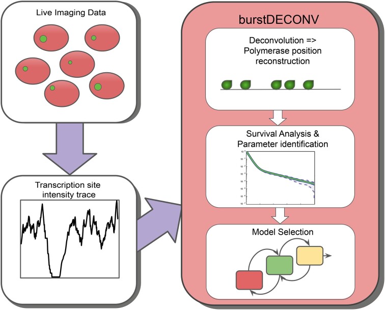
Graphical Abstract.

BurstDECONV deconvolves live cell transcription imaging data to reconstruct each polymerase initiation event. By analyzing the distribution of waiting time between successive initiation events, we decrypt the number of rate-limiting steps driving transcription and accordingly, choose the best model that recapitulates the different promoter states and their stochastic switching.

INTRODUCTION

The observation of transcription in live cells using methods such as MS2/MCP system (1,2) revealed that in most prokaryotic and eukaryotic cells, transcription is discontinuous and undergoes alternative periods of activity and inactivity, governed by stochastic laws. This phenomenon was called transcriptional bursting (3–8). The underlying mechanisms are complex because, even at the steady state, promoters can adopt multiple active and inactive states with distinct timescales and transition schemes, which modulate the variability of expression levels in single cells in non-trivial ways (9–12). Hence, it is necessary to infer these states and timescales from observations. The results of such inference are important as they provide insights into the molecular mechanisms underlying promoter dynamics and transcriptional regulation.

Transcriptional bursting with multiple active and inactive promoter states can be modeled using Finite-State Markov Models (FSMM) defined by a set of promoter states and by the rates of stochastic transitions between these states (13). The simplest FSMM, the random telegraph model, has two states and explains the alternation of transcriptionally active and inactive periods observed in transcriptional outputs (14). Commonly used to describe the bursting of prokaryote and less complex eukaryote promoters (6,15,16), this model fails to explain more complex eukaryote transcription mechanisms, as we and others have recently shown using live imaging data of human cell lines and Drosophila embryos (17–20). In this case, bursting models involving more than two states are required (21,22).

We must emphasize that the identification of models and rates describing the observed transcription dynamics is not merely a phenomenological description. Indeed, this gives direct access to key regulatory mechanisms at the molecular level. A variety of perturbation experiments have indicated that the states in the kinetic models correspond to well defined biochemical states of the promoter, and specific chromatin features and binding profiles of given transcription factors (e.g. assembled pre-initiation complex PIC, or TATA Binding Protein-bound, or nucleosome occupied promoter; (7,16,23–25)). Furthermore, recent advances in cryo-electron microscopy, as well as single molecule genomic methods (26) have revealed that promoters can be found in a multitude of molecular states as they undergo transcription initiation or early elongation (27–31). However, it is often difficult to figure out from molecular experiments which state is rate-limiting, and this is a key question as the rate-limiting steps are likely points of regulation. Live cell transcription imaging fills this gap, and robust methods to infer promoter dynamics from such data are thus essential for understanding the basic mechanisms of transcriptional control.

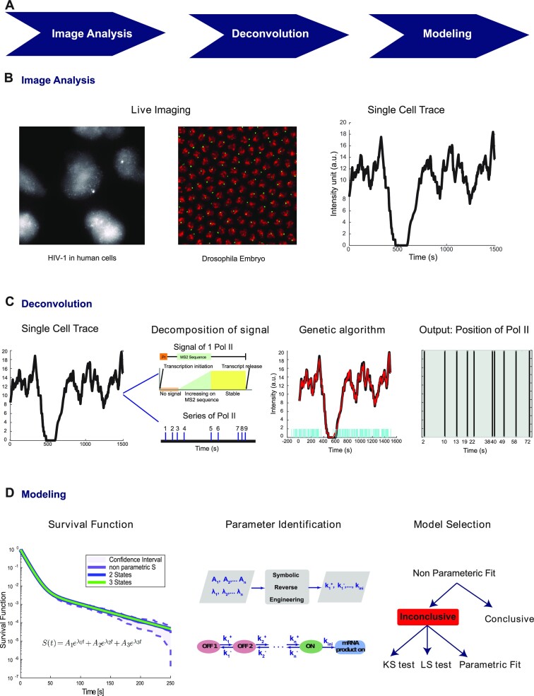
In order to decode single cell transcriptional traces, we developed BurstDECONV, a deconvolution based method for reconstructing FSMMs from live transcription imaging using RNA tagging. An overview of this method is presented in Figure 1. BurstDECONV first decomposes single cell MS2/MCP live imaging data into individual transcription initiation temporal events (Figure 1 C). This information is model agnostic and represents a comprehensive spatio-temporal map of transcription that can be used for multiple studies: identifying multiple temporal and spatial scales and kinetic parameters, testing the synchronicity or the correlation of transcription sites, detecting extrinsic noise events, and performing model selection and inference (19,20). In a second step, BurstDECONV computes the survival function characterizing the distribution of waiting times between successive polymerase initiation events (Figure 1D). Finally, multiexponential parametric survival models are inferred and mapped to FSMM kinetic promoter models. The number of exponentials required to fit the survival functions corresponds to the number of promoter states in the model, and this facilitates model comparison and selection (Figures 1D and 3). BurstDECONV has also been successfully applied to extracting transition rate parameters from real data (19,20) in human cells and Drosophila embryos. Importantly, this method revealed an alternative model of promoter pausing, described as facultative pausing, which could not be characterized by other live- or fixed-sample approaches.

Figure 1.

Overview of the live cell transcription imaging pipeline. (A) Workflow of the pipeline. (B) Movies are segmented to extract single cell signals. (C) For each single cell we compute the sequence of polymerase positions. (D) Single cell data is used to compute the survival function and identify parameters of transcriptional bursting models.

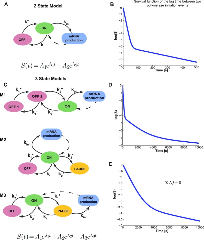
Figure 3.

Finite-State Markov Models of transcription dynamics. (A) Model depicting two promoter states, and with the respective transition rates. (B) The theoretical survival function corrresponding to the two-state exponential model has two timescales. The two separated timescales can be distinguished as two distinct slopes, piecewise in the semi-logarithmic representation. (C) Three-state models with different transition schemes. (D) The theoretical survival function of the three state models M₁, M₂ is a sum of three exponentials with no constraints on the amplitudes A_i. The three separated timescales can be distinguished as three distinct slopes, piecewise in the semi-logarithmic representation. These two models have the same type of survival function and can not be discriminated by BurstDECONV only. (E) The theoretical survival function of the three state model M₃ is a sum of three exponentials with constrains on the amplitudes A_i and exponents λ_i. Only two free timescales can be distinguished in the semi-logarithmic representation.

We have performed a comparative benchmarking in which BurstDECONV was tested along with auto-correlation (32,33) and Hidden Markov Model (HMM) (34–36) methods, two other approaches previously employed for analysing transcriptional bursting data. Whenever comparison was possible, we found that the parameter reconstruction by BurstDECONV is significantly more accurate than by all other methods. Moreover, our method is precise for wide ranges of values of kinetic parameters of transcription processes. By combining short and long movies, we are able to quantify processes with timescales from seconds to days. This extremely wide dynamic range was not accessible with the previous quantitative live cell transcription imaging approaches.

Thus BurstDECONV proves to be a very effective tool for analysing live cell transcription, paving the way to exciting discoveries in the field of transcriptional control. For a wide usage, we provide Matlab and Python implementations of our method, and a user-friendly graphical interface that fits data to a variety of two and three state promoter models.

MATERIALS AND METHODS

Short, high resolution movie deconvolution

The MS2 signal from one transcription site is modeled as:

(1)

where x_pol is the signal from one polymerase and t_i are the successive initiation times.

The initiation times are discretised , where δ = D_min/V_pol, with D_min a minimal inter-polymerase distance (in bp) and V_pol the polymerase speed (in bp/s) that we assume constant. The entire sequence of initiation times is then coded as a fixed size binary string , where N_max = T/δ, T is the movie length.

If x_cal(t) is the observed signal, calibrated in polymerase numbers, we find B and thus t_i by least-squares regression using a genetic algorithm GA and the objective function:

(2)

where Δ is the movie time resolution and N_frames is the number of frames, T = N_framesΔ.

The GA optimization follows four steps: estimating the amount of polymerases, generating an initial population, applying the genetic algorithm and the final local optimization. We estimate the number of polymerases N_pol as the ratio of integral intensities of the experimental signal and of the single polymerase signal. The resulting rough estimation is used to accelerate next steps. Then we prepare an initial population of polymerase positions. Starting with a binary string B with N_max ’0’s, we randomly pick N_pol positions and change them into ’1’s. After the preparation of the initial population, we use the genetic algorithm (MATLAB built-in function ga or a modified Python function pygad.GA, depending on the implementation) to optimize the objective function. At each step, the genetic algorithm solver randomly selects a sub-population of parental individuals from which it produces the next generation by recombination, crossover and mutation. Over successive generations, the population keeps the best generated solutions and ‘evolves’ towards an optimal solution. The local optimization further decreases the objective function by displacing the polymerase positions a few steps to the right or to the left.

After optimization, the residuals x(kΔ; B_optimal) − x_cal(kΔ) for all the transcription sites in the same movie are used for estimating the noise in the signal. We systematically find that noise is heteroscedastic with a variance depending non-linearly on the signal amplitude. We use cubic polynomial regression to approximate the dependence of the noise variance on the signal:

(3)

The waiting times τ_i = t_{i + 1} − t_i, defined as intervals between successive initiation events coming from all the transcription sites in the movie, are considered as realizations of the same random variable τ. The survival function is defined as

(4)

and estimated (non-parametrically) using the Kaplan-Meyer method (37) from the pooled series coming from all the transcription sites in the same movie.

Space dependent analysis can also be performed, by pooling the transcription sites region-wise (a prior spatial segmentation is needed).

We model the survival function using the multi-exponential family

(5)

where , λ_i < 0, 1 ≤ i ≤ n_exp.

The parametric estimate of the survival function is obtained by least square regression with an objective function that combines linear and logarithmic scales:

(6)

where S(t) is defined by (4), S_KM(t) is the non-parametric estimate of the survival function, 0 ≤ α ≤ 1 is a weight representing the relative importance of the linear scale compared to the logarithmic scale in the estimate of the survival function.

The use of linear and logarithmic scales was motivated by the fact that short timescales responsible of the large initial drop in the survival function are well captured by the linear scale, whereas longer timescales responsible for the smaller decrease in the tail of the survival function are well captured by the logarithmic scale.

The multi-exponential least-squares regression is performed for several values of the number of exponentials n_exp. The selection of the number of exponentials is based on three criteria: the optimal value of , the Kolmogorov–Smirnov test using the optimal as reference distribution and the uncertainty of the parameters obtained by considering optimal and close to optimal solutions (Figure 5).

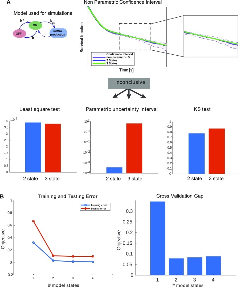
Figure 5.

Selection of the number of exponentials in multi-exponential survival models. (A) The number of exponentials n_exp in the multi-exponential survival model is first selected using the Greenwood confidence interval for the Kaplan-Meyer non-parametric estimator. One verifies that the optimal parametric estimate is included in the confidence interval of the non-parametric estimate, for increasing n_exp starting with n_exp = 1. The selected n_exp value is the first one that satisfies this condition. If the result is inconclusive (borderline), we evaluate the training error by using the least-square error or the Kolmogorov–Smirnov test, and the overfitting by using the width of the parametric uncertainty intervals. The selected n_exp is the first one that has similar training error and lower parametric uncertainty than n_exp + 1. (B) Cross-validation. The dataset (set of nuclei) obtained from a two-state ground truth model (dataset D6) is split into a training and validation subsets. Then the model capacity is increased by increasing n_exp. Both training and testing errors decrease with n_exp but the difference between the two (the cross validation gap) has a minimum at the ground truth. The cross-validation can be used for selection when the number of samples (nuclei) is large enough.

Combining two movies

The second version of the method uses two movies. The short high resolution movie is processed exactly as in the first method, resulting in the survival function S₁(t). The transcription site signals from the long low resolution movie are thresholded. The sub-threshold intervals are used to estimate a survival function S₂(t). Given that S₁(t) misses waiting times longer than the short movie length T and that S₂(t) misses waiting times shorter than T_min (estimated as the sum of the long movie resolution and the single polymerase signal duration), an interpretation of these two survival functions in terms of conditional probabilities is appropriate:

(7)

Using the total probability theorem we obtain the multiple time scale survival function

(8)

where and .

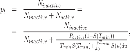
p _l is estimated using the formula (see (19)):

(9)

where N_inactive is the number sub-threshold intervals (resolved and countable), N_active is the number of waiting times inside over-threshold intervals (not resolved), P_active is the probability to be over threshold (estimated as the time fraction from total that is over threshold) in the long movie signals; for this estimate we use S(t) ≈ S₁(t) for t < T_min.

p _s is optimised to minimize the gap between the short time and long time survival function branches in (8). The estimate of the gap uses interpolation and is possible only if there is an overlap between S₁(t) and S₂(t).

The multi-exponential parametric estimate of the survival function is now performed using the multiple time scale survival function (8).

Rate parameter identifiability

Both versions (short movie and short-long movie) of our method end with the identification of the FSMM rate parameters. This identification is possible symbolically, using analytical formulas that relate the multi-exponential parameters to the rate parameters.

For the sake of completeness we introduce, in the simplified case of the random telegraph model, the mathematical objects needed for solving this problem. Some solutions for FSMM with 2, 3, and 4 states can be found in (19). The algorithmic solution for an arbitrary number of states will be provided in a separate publication.

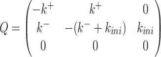
Let us denote by 1 and 2 the states and of the random telegraph model, respectively. In order to study transcription initiation we add to the model a third state 3 representing the initiation event. The extended three states FSMM is defined by the transition rate matrix whose elements are the transition rates between the states of this model. For instance, the matrix element Q₁₂ represents the transition rate from to , which is k⁺. Furthermore, we are interested in the waiting time to initiation, so we decide to stop the FSMM whenever we reach the state 3, which means that all the elements on the last row of are zero. The elements of the transition rate matrix sum to zero on any row, therefore

The vector

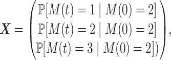where M(t) is the state of the FSMM at the time t satisfies the master equation:

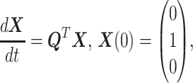(10)

where stands for the transpose of .

Eq. (10) is equivalent to

(11)

(12)

where

The waiting time w between successive initiation events represents the first return time in the state 3 after starting in the state 3 (this is equivalent to starting in 2 because after initiation the promoter is immediately freed and gets to the state). The survival function is then , which shows that one can compute the survival function by solving the linear system of ODEs (11) with the initial conditions from (10). Interestingly, for constant parameters, the distribution of w does not change in time (it is the same during transient and steady state gene expression). In other words, the sequence of initiation events is a renewal process.

The solution of (11) reads

(13)

(14)

where , are eigenvectors and λ₁, λ₂ are eigenvalues of the matrix , and C₁, C₂ are the solutions of the system

(15)

Furthermore,

(16)

From (14) and (12)

(17)

Eqs. (16), (15) and (17) provide the solution of the direct problem that consists in computing the survival function parameters given the transition rate parameters. The inverse problem consists in computing the rate parameters k⁺, k⁻, k_ini given the independent survival function parameters A₁, λ₁, λ₂. The rate parameters are identifiable if and only if the inverse problem is well posed, i.e. it has a unique solution.

The inverse problem for the random telegraph model corresponds to solving the system

(18)

(19)

(20)

Eqs. (18) and (19) are the Vieta’s formulas, resulting from the fact that λ₁, λ₂ are the solutions of the characteristic equation of the matrix . Eq. (20) follows from (15) and (17).

For the random telegraph model, the solution of the inverse problem is unique and the transition rate parameters are expressed in terms of symmetric rational functions in the variables λ₁, λ₂, A₁, A₂, i.e. ratios of polynomials invariant with respect to permutations of these variables. More precisely,

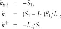(21)

where S₁ = A₁λ₁ + A₂λ₂, L₁ = λ₁ + λ₂, L₂ = λ₁λ₂, are symmetric polynomials.

More generally, one can show that whenever the inverse problem has a unique solution, this can be written in terms of symmetric polynomials. Of course, the inverse problem can also have no solutions, or have an infinity of solutions.

The question of model and parameter identifiability can be decomposed into two steps. First, the survival function parameters are uncertain because they are obtained from data. Second, the inverse problem, consisting in identifying the model and its kinetic parameters for the survival function parameters can be not well posed and have infinitely many solutions. This source of uncertainty can be also addressed using symbolic methods (19). There are several situations of symbolic non-identifiability/uncertainty:

• Model non-identifibility/uncertainty. Model parameters are uniquely determined for each model, but different models give exactly the same survival function with different parameters (the case of models M₁, M₂, Figure 3C).

• Parameter non-identifiability/uncertainty. Model kinetic parameters leading to the same survival function form smooth manifolds, meaning that some of them are free. Concurrently, multi-exponential parameters of the survival function are constrained, meaning that there are less free parameters of the multi-exponential survival function (the case of the model M₃, Figure 3C).

In both cases of non-identifiability/uncertainty, more data is needed in order to directly identify one or several parameters. We have implemented this strategy in (19,20) where, using chromatin immunoprecipitation or genetic perturbations of pausing, the parameter was shown to correspond to exit from proximal pausing, indicating that the model M₂ should be preferred to M₁.

Determining the polymerase dwell time from the signal autocorrelation

The signal autocorrelation function is defined as R(t, t′) = Cov(x(t), x(t′)), where x(t) is the single site MS2 signal. For a stationary MS2 signal, this function depends only on τ = t′ − t and factorizes as:

(22)

where d is the dwell time, k contains all model parameters including the dwell time (for instance k = (k⁺, k⁻, k_ini, d) for the random telegraph model), H(x) = −xθ( − x), is the Heaviside function (see (32) for a derivation).

The determination of the dwell time results from fitting the theoretical model (22) to the empirical autocorrelation function resulting from data. The test of this method is illustrated in the Supplementary Table S1.

It turns out from (22) that the autocorrelation function R depends strongly on d and only weakly on the other parameters k. For this reason d is precise, whereas k is uncertain when estimated from R.

RESULTS

Principles and workflow

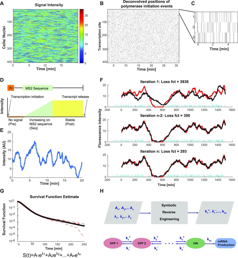
The input data for our model are live imaging data of nascent transcription, with nascent RNAs labeled with a fluorescent tag. As test samples, we used MS2/MCP data collected from either cultured human cells or Drosophila early embryos. This labelling method is bipartite, with an RNA containing MS2 repeats of various lengths, detected by an RNA binding protein, here MCP, fused to a fluorescent protein (Figure 2D). After live imaging, MS2/MCP fluorescent signals of single transcription sites (temporal traces) are extracted through image analysis methods described in (18,20) that track each transcription site in 3D in order to extract the intensity of the MS2 signal over time. For each movie we produce an intensity matrix whose rows and columns represent transcription sites and time, respectively (Figure 2A). Because we wish to separate individual transcription initiation events we use movies with high temporal resolutions (typically 3–4 s) and the sequence of transcription initiation events is reconstructed independently for each transcription site (Figure 2B, C). The MS2/MCP fluorescent signals are calibrated to be expressed as polymerase numbers. In order to decompose the signal observed from multiple polymerases (Figure 2E) into initiation events, we first consider the signal expected from a single polymerase, schematized in Figure 2D. The single polymerase pattern is computed from n_seq, n_post, V_pol and t_a, representing the length in base pairs of the MS2 sequence, the remaining length after the MS2 sequence until the polyA site, the polymerase elongation speed and the 3’-end processing/polyadenylation time, respectively. In this notation, the polymerase dwell time on the DNA is (n_seq + n_post)/V_pol + t_a. In this model, we consider that a polymerase, once initiated, will continue transcription until it reaches the 3’-end. The estimated initiation times are obtained by least squares regression using a global genetic algorithm, followed by local optimization (Figure 2F). Multi-exponential parametric estimates of the survival function are then used to characterize the distribution of the waiting times between successive initiation events for the entire population of sites (see Figure 2G and Materials and Methods). The multi-exponential regression proposes one, two, or more exponentials. The number of exponentials corresponds to the number of states in the FSMM (Figure 3). Finally, comparison of the exponentials found by regression to the analytic solutions of the master equation satisfied by the survival function allows us to write explicit formulas for FSSM parameters in terms of the regression results (Figure 2H).

Figure 2.

Overview of various steps of BurstDECONV. (A) Heatmap of the signal extracted from a high resolution movie. Each row represents a transcription site intensity in time (x-axis). The colour bar depicts the number of nascent RNA. (B) Timeline chart representing the transcription initiation events obtained for each corresponding transcription site intensity trace after performing deconvolution using the genetic algorithm. (C) Close up of the timeline chart. Each bar represents a single event; successive events are separated by waiting times. (D) The RNA tagging construct and its corresponding signal generated from a single polymerase. The orange box labeled Pr represents the promoter site where transcription initiation takes place. The MS2 sequence is located a few bases downstream of the promoter region. The signal profile is shown below the construct. (E) Intensity trace from one transcription site. (F) Example of polymerase positions reconstructing the transcription site intensity trace in the last three generations of the genetic algorithm. The red trace is the intensity trace that is to be reconstructed. The black trace is the reconstructed signal from the predicted polymerase positions (represented with blue bars). (G) Survival function estimated from the waiting times between the predicted polymerases. The dotted red curve represents the Greenwood confidence interval of the survival function. We obtain both non-parametric survival function (depicted with red circles) by Kaplan-Meier method, and the parametric survival function by least square regression (depicted with the black curve). The parametric survival function is a sum of N exponentials. (H) The various coefficients of the parametric survival function are used to obtain the model parameters (switching rates between different states) through symbolic reverse engineering.

A few examples of FSMMs are represented in Figure 3. The random telegraph model (Figure 3A) contains two states: the state corresponding to active transcription, modeled by Poissonian initiation with constant initiation rate k_ini; and the inactive state where no initiation events are observed. As the two state random telegraph model is generally too simplistic to fully describe the complexity of the transcription process (18,38,39), we also envisaged more complex models with three states, comprising two inactive states (models M₁, M₂ and M₃). In the model M₁ (Figure 3C), an inactive promoter occupying the state can become active (state ON) or switch to a deeper inactive state . Inactive states represent various molecular states of the promoter, such as chromatin states or assembly stages of the transcription pre-initiation complex (PIC). In the model M₂ (Figure 3C), the second inactive state was interpreted as proximal pausing. This interpretation is based on the experimental manipulation of pausing (in cis or in trans) that we performed with model paused promoters such as HIV-1 in human cells or developmental core promoters in Drosophila embryos (19,20). In the model M₂ the transition from to is stochastic, therefore pausing is facultative. This is at odds with the traditional obligatory pausing model M₃ (Figure 3C) in which the pausing occurs after initiation and systematically prevents elongation, as usually depicted in the literature (40). The model M₃ predicts a special type of survival function whose multi-exponential parameters are constrained by an additional relationship (see Figure 3E and (19)).

The inverse problem consisting in computing the model kinetic parameters from the survival function parameters (A_i, λ_i), 1 ≤ i ≤ n, is well posed when it has a unique solution for all survival function parameters satisfying the constraints . This is the case for the random telegraph model, for the models M₁, M₂, for a family of models of arbitrary size discussed in (19), but not for the model M₃. For M₃, the survival function parameters are constrained by one bilinear equation in A_i and λ_i (see Materials and Methods and Figure 3); furthermore, in this case the inverse problem has infinitely many solutions, that depend on one free parameter.

Artificial data shows the robustness of BurstDECONV

In order to benchmark the method we use a collection of artificially generated datasets. These datasets consist of MS2 signals from N transcription sites. The models and corresponding parameter sets are given in Table 1, and they are chosen to mimic a variety of real biological situations. Indeed, the parameter sets simulate observations of wild type and mutated snail (D2,D3,D5,D7,D9) or Kruppel (D1,D4,D8) Drosophila promoters studied in (20), or from HIV-1 promoters inserted in Hela reporter cell line in various configurations (notably with and without the viral transactivator Tat; D12–14) studied in (19). We have added a few more parameter sets corresponding to the wild-type and mutant human EEF1A promoters inserted in human cell lines (D6;D10–11). These data cover a large range of expression levels, and correspond to promoters having two or three rate-limiting steps, and being mostly, or only episodically, active.

Table 1.

FSMM parameters used to generate the artificial datasets. Furthermore, the MS2 sequence and elongation rate parameters were n_seq = 1292 bp (24×MS2), n_post = 4526 bp, V_pol = 45 bp × s⁻¹ for D1–5 and D7–9,n_seq = 5800 bp (128×MS2), n_post = 8300 bp, V_pol = 67 bp × s⁻¹ for D6 and D10–14. D1–5 and D7–9 parameters come from the study of Drosophila promoters in (20). D12–14 is based on estimates of HIV-1 transcription bursting in human cells studied in (19). D6 and D10–11 come from estimates of bursting from wild-type and mutated EEF1A promoters inserted in human cell lines

Dataset/Ref.	Parameters
2 states	k +[s−1]		k −[s−1]		k ini [s−1]
D1 (20)	0.02036		0.00150		0.11432
D2 (20)	0.01117		0.00593		0.07637
D3 (20)	0.01189		0.01430		0.07745
D4 (20)	0.02439		0.00144		0.13397
D5 (20)	0.04169		0.00414		0.11277
D6	0.00484		0.00025		0.113
3 states M2					k ini [s−1]
D7 (20)	0.01426	0.00339	0.06553	0.05751	0.17102
D8 (20)	0.00661	0.00013	0.05772	0.01054	0.13201
D9 (20)	0.00332	5.3 × 10−5	0.05804	0.00586	0.13119
D10	0.0001	2.3 × 10−5	0.00091	0.00024	0.019
D11	0.00023	3.2 × 10−5	0.0011	0.00019	0.018
D12 (19)	0.0015	4.9 × 10−5	0.01	0.0043	0.17
D13 (19)	0.00015	0.00031	0.0012	0.0028	0.1
D14 (19)	6 × 10−5	0.00035	0.00089	0.003	0.063

The artificial data was generated using the parameter estimates obtained with real data. Using the Gillespie algorithm we generated N independent trajectories of the FSMM that provide the initiation events over a time interval T corresponding to the movie length. Then, we use the single polymerase patterns to compute the MS2 signal. The single polymerase patterns correspond to 24xMS2 and 128xMS2 constructions in Drosophila and in human cell lines, respectively (see (18–20)). For more realism, we add noise to this signal. In analogy to real data, we use Gaussian heteroscedastic noise (see (19) and Material and Methods).

In order to evaluate the accuracy of the parameter reconstruction we use the logarithmic error defined as |log₁₀(k_r/k_true)|, where k_r, k_true are the reconstructed parameter and their true value, respectively. Errors were considered unacceptable if they correspond to one order of magnitude, i.e. if the logarithmic error is larger than one.

BurstDECONV combines short high resolution with long low resolution movies to cover widely distributed timescales

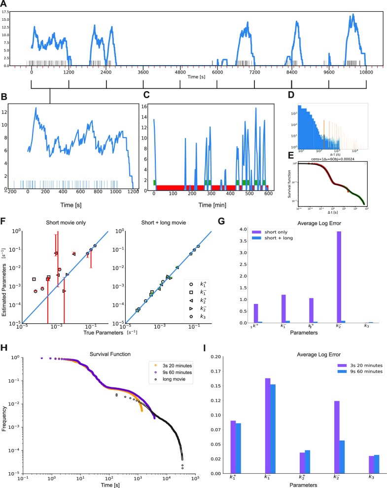
Transcription bursting is a complex phenomenon involving processes with multiple timescales distributed over many orders of magnitudes (8,18). The movie length sets the upper bound of the timescales of processes that can be identified using live cell RNA imaging data. A short movie may fail to detect slow processes that involve long waiting times. In order to test this we have used models that have timescales ranging from 1s to 10⁴s. Deconvolution of a short (20 min) signal (Figure 4 B) results in mediocre parameter reconstruction (Figure 4 F) and as expected, errors were larger for smaller kinetic parameters (large timescales). In order to illustrate this effect we have used the dataset D14 that includes very long waiting times (very small values of the parameters and ).

Figure 4.

Combining short and long movies. (A) Simulated long duration signal using the three-state model M₂ and high temporal resolution, parameters corresponding to dataset D14. The timeline with black markers represent polymerase start time positions. The transcription site signal is represented in blue, using short movie high temporal resolution. The x-axis major tick marks in black (every 1200 seconds) represent the duration of a high resolution short movie (1 stack every 3 s for 20 min). The minor ticks in red represent 3 min marks, i.e. the resolution of a long duration movie (1 stack every 3 min). (B) Simulated low resolution short movie using the model M₂. Blue bars represent polymerase positions found by GA after deconvolution (blow-up start of the signal from A). (C) Low resolution long movie with thresholding to extract off periods or waiting times. (D) Histogram of length of waiting times obtained from short movies (in blue) and long movies (in orange). (E) Matched Survival function of the long (green) and short movie (red) with overlap in the middle. (F) Accuracy of parameter reconstruction of the model M₂ for the parameter sets D12–14 in Table 1 using only a short movie and a short + long movie. (G) Average logarithmic error of the parameter reconstruction of the model M₂ for the parameter sets D12–14 in Table 1 using a short movie (20 min every 3 s) combined or not with a long movie (10 h every 3 min). (H) Long and short movie survival functions and their overlap for different lengths and resolutions of the short movie. (I) Average logarithmic error of the parameter reconstruction of the model M₂ for the parameter sets D12–14 in Table 1 for different durations and resolutions of the short movie.

Due to bleaching of the signal, obtaining long movies (in the h scale) while imaging with a high temporal resolution of few seconds is extremely challenging.

Instead, we designed a version of BurstDECONV that combines short, high resolution movies, and long, low resolution movies. The first step consists in deconvolution of the short high-resolution movies and computation of their survival function. The second step processes the long movies, which last typically 10 h with a temporal resolution of 3 min. In this case, active and inactive periods are defined directly by considering the parts of the MS2 signal that are above and below a threshold, respectively, with the threshold corresponding to the brightness of 2–3 RNAs (Figure 4C). By thresholding, we miss the short waiting times between transcription events that occur during active periods, and we thus count only the long waiting times corresponding to inactive periods (i.e. waiting times greater than the dwell time of a polymerase, defined as the total time length of the signal generated by a single polymerase). The distribution of the long waiting times overlaps that of short waiting times obtained from the short movies (Figure 4D). This overlap permits us to reconstruct a multiscale survival function that covers many orders of magnitude in time (see Figure 4E and (19)). The multiscale survival function is then used for multi-exponential regression and provides the kinetic parameters of the model. The combination of the two movie types permits a good reconstruction of these parameters (Figure 4G).

The length of the short movie is critical for ensuring the overlap of the short and long timescale survival functions and an accurate parameter reconstruction. Interestingly, longer short movie with lower temporal resolution (60 min length with frames every 9 s, instead of every 3s for 20 min) can ensure a better reconstruction of the model parameters (Figures 4H, I), even with initiation rates (k_ini) in the range of 3 s. This provides useful guidelines for the experimental design and imaging conditions.

Thus, BurstDECONV allows to uncover processes with a remarkable distribution of timescales ranging from seconds to days.

BurstDeconv determines the number of states of the kinetic promoter model

A key question when analyzing live cell transcription imaging experiments, is the choice of the model used to fit the data. Instead of arbitrarily employing the simple random telegraph promoter model, our procedure uses the multi-exponential fit of the waiting time data to determine the number of promoter states that should be considered. We recall that, except for special cases when the spectrum of the matrix is degenerate, the number of states in the transcriptional bursting model is equal to the number of exponentials n_exp in the multi-exponential fit.

In order to compare models with different n_exp we use several indicators for the goodness of fit (Figure 5A). The experimental estimate of the survival function by the Kaplan–Meyer method provides a confidence interval based on Greenwood’s formula (20). A first accuracy test consists in checking that the optimal parametric estimate of the survival function lies within this confidence interval. The Kolmogorov–Smirnov (KS) test and the optimal value of the objective function (the mean squared deviation; see Material and Methods for a definition) provide alternative measures of the quantitative goodness of fit. The Greenwood’s confidence interval and KS methods do not take into account errors resulting from the imperfect join of the short and long movie survival functions. Therefore, the only goodness of fit measure when one also uses long movies is the value of the objective function .

The goodness of fit systematically increases with n_exp and one would like to know when to stop. The stopping criteria can be based on parsimony (Figure 5 A): choose the less complex model (smallest n_exp) whose goodness of fit does not differ significantly from the next more complex one. An alternative strategy can use cross-validation. We illustrate cross-validation by splitting the artificial data in a training and a validation subset. Both training error and validation error decrease with n_exp. However, their difference (the validation gap) has a minimum. The optimal n_exp corresponds to training and validation errors that are as close as possible, i.e. corresponding to the minimal validation gap. A large validation gap indicates either underfitting (when both training and validation errors are large) or overfitting (Figure 5 B).

Cross-validation is usually difficult to set in practice when the number of available cells is not large enough. In this case we estimate overfitting by parametric uncertainty. Indeed, an overly complex model can fit data equally well for different values of its parameters. We use optimal and close to optimal solutions to define uncertainty intervals that contain the parameters leading to a close to optimal fit. We then gradually increase n_exp until the goodness of fit (training error) becomes sufficiently small while the uncertainty parametric intervals are not large (Figure 5A).

Alternative model selection procedures, based on hierarchical Bayesian learning have been proposed for obtaining the parametric survival function and the number of exponentials (chapter 5 of (41)). Their practical implementation will be tested in future work.

BurstDECONV is robust against error and suboptimal experimental designs

Robustness against changes in calibration

In this method and in any quantitative method based on live cell transcription imaging, the polymerase loading rate (k_ini) can be determined only if the signal intensity is expressed in units of full-length transcripts.

The calibration is performed by dividing the transcription site signal intensity by the calibration factor that is defined as the contribution to intensity of a single RNA molecule. This factor can be computed in different ways. In order to calibrate fluorescent signals from live Drosophila embryo imaging, we used single-molecule hybridization experiments (smFISH) as described in (20). In human cell lines, we collected right after the end of the movie one 3D stack—termed calibration stack—with increased laser intensity, which similarly allowed reliable detection and quantification of the brightness of individual RNA molecules (18,19).

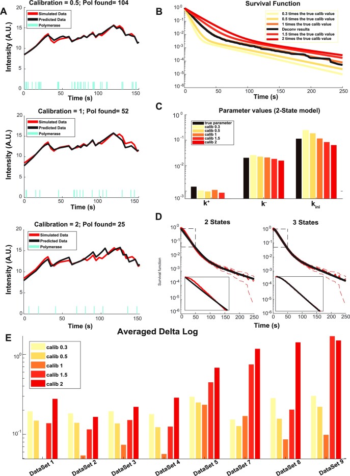
We illustrate the importance of the calibration factor by testing the effect of altering it in artificial data (Figure 6). Decreasing the calibration factor corresponds to underestimating the contribution of one RNA to the signal and corresponds to more polymerases to model the same signal (Figure 6A). This also has an influence on the survival function, because more polymerases mean shorter waiting times between successive initiation events (Figure 6B). Increasing the calibration factor leads to decreased estimates of all kinetic parameters (Figure 6C). As expected, the polymerase initiation rate (parameter k_ini in the random telegraph model) scales like the inverse of the calibration factor (Figure 6C). The effect of the calibration factor on the switching parameters (k⁺ and k⁻ in the random telegraph model) is asymmetric. It is weaker when the calibration factor is less than optimal and larger for calibration factor larger than optimal (Figure 6E). In other words overestimating the one polymerase signal leads to larger reconstruction errors than underestimating it. A possible explanation of this effect is that increasing the calibration factor reduces the apparent number of initiation events which renders the identification of the switching periods less reliable. In order to illustrate these effects we have used the dataset D1. This dataset (together with D4 that is very similar) proved to be the most sensitive to calibration, as in this case a twofold increase of the calibration factor with respect to the optimal value leads to selecting a three states instead of the ground truth two states model, see Figure 6D. This dataset corresponds to a highly active promoter as k⁻ and k⁺ are small and large, respectively.

Figure 6.

Testing the effect of a change in the calibration factor. (A) Simulated signal for a two-state model, dataset D1 in Table 1, for different values of the calibration factor. The cyan timeline bars indicate the start time positions. The simulated transcription site signal is represented in red. The reconstructed signal (after deconvolution) is represented in black. For the ground truth, the number of simulated polymerases is 52 and the calibration factor is one. (B) Survival functions reconstructed for different values of the calibration factor (two-state model, dataset D1 in Table 1). (C) Reconstructed parameter values for different calibration factors (two-state model, dataset D1 in Table 1). (D) Nonparametric survival function compared to parametric 2- and 3-exponential functions for a calibration factor = 2. Doubling the calibration factor with respect to the ground truth can mistakenly lead to a change in the model selection from two (ground truth, falsified by the confidence interval criterion) to three states. (E) Average logarithmic parameter reconstruction error for various datasets and calibration factors.

Robustness against changes in polymerase speed and dwell time

In our method, the polymerase speed is considered to be known. Changing this parameter is roughly equivalent to changing the polymerase dwell time and has effects on the number of polymerases (and loading rate parameter) opposed to changing the calibration.

Robustness against changes in time resolution

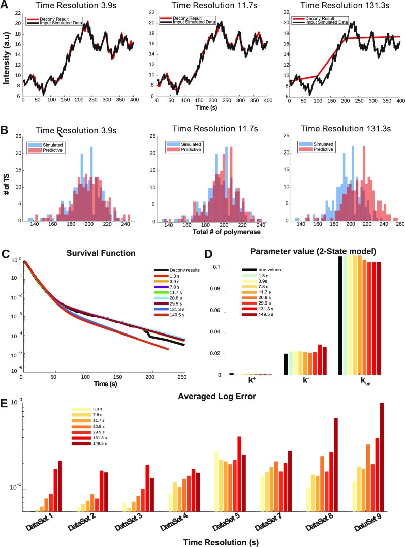
A low resolution movie provides poor representations of the MS2 intensity (Figure 7A). The deconvolution algorithm tends to interpret local drops in the MS2 signal as an state. However, these drops and the corresponding states may be missed for very low resolutions (such as 131.3 s in Figure 7A). Missing states lead to a larger number of predicted polymerase positions (Figure 7 B), steeper survival functions (Figure 7C) and errors mostly in the to transition rates (parameter k⁻ in Figure 7D). The shorter timescales, corresponding to the parameters k⁺, k_ini are less affected. The critical resolution producing large errors in the number of polymerases, survival function and kinetic parameters is close to the polymerase dwell time. We compared the results obtained by our procedure on artificial datasets resampled with various temporal resolutions and found that the method is robust and tolerates resolutions (11–20 s) much lower than the ones currently employed (3–3.9 s). Thus, there is not significant gain when imaging every 3–4 s compared to imaging every 11–20 s. This again provides important guidelines to design optimal imaging conditions.

Figure 7.

Testing the effect of a change in the movie time resolution. (A) Simulated and reconstructed signal for different time resolutions, for a two state model, dataset D1 in Table 1. The simulated transcription site signal is represented in black. The same signal is resampled with different rates and then reconstructed by deconvolution. The reconstructed signal (after deconvolution and with different sampling rates) is represented in red. (B) Histograms of the number of polymerases per analysed site for different time resolutions. (C) The reconstructed survival functions for different time resolutions. (D) Average logarithmic parametric reconstruction error for different time resolutions and kinetic parameters (dataset D1). (E) Average logarithmic error for different datasets and time resolutions.

Robustness against noise in the data

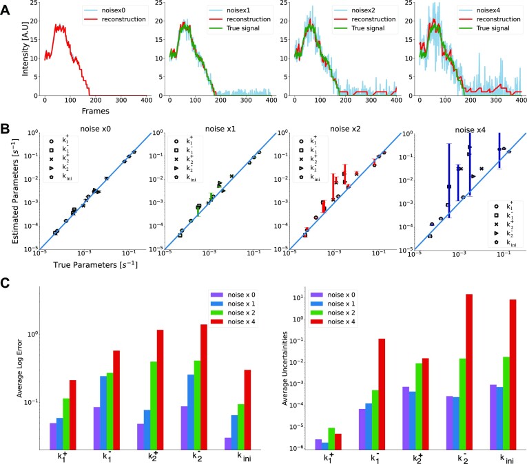
In order to simulate a noise that resembles real experimental data, we analyzed the variance of the residuals resulting from the least-squares fitting. We have found that residuals are normally distributed with a variance increasing with the level of the predicted signal, which means that the experimental noise is heteroscedastic. A third order polynomial fitting was enough for approximating this dependence (see Materials and Methods). We thus have added Gaussian noise to the artificial data, whose variance has the same polynomial dependence on the mean as the experimental data. We have found that even for a noise amplitude multiplied by four with respect to the experimental values, BurstDECONV is able to reconstruct the parameter values used for the simulation (Figure 8). The accuracy is very good for experimental noise amplitudes. To some extent, the noise in the signal is averaged by the least-squares optimization step and therefore no noise subtraction or estimation is needed for the parametric model reconstruction in BurstDECONV. In order to illustrate these effects we have used the datasets D12–14 because they have multiple, well separated waiting times, which allow us to test the effect of noise on different timescales.

Figure 8.

Robustness of the method against noise. All the simulations were performed using a 3-states model M₂ (Datasets D12-14 in Table1). (A) Reconstructed signal (shown in red) obtained using deconvolution from noisy artificial data (shown in blue). The artificial signal without noise is shown in green. Noise x0 represents the signal without any noise added to it and noise x1 is obtained by adding heteroscedastic noise to noise x0 equivalent to the one estimated from cultured human cells. noise x2 and x4 correspond to noise standard deviations two and four times larger, respectively. (B) Parameters reconstructed by the pipeline vs the true parameters used to simulate the artificial data for model M₂ datasets D12–14 in Table 1. (C) Logarithmic parametric reconstruction error D12–14 (left) Average uncertainty in the parameters (right).

Robustness against the detection limit

It is very common in live cell imaging to have a background noise signal that sets a detection limit. To recreate this effect, we have added a supplementary component to the noise, which is independent of the MS2 signal. We tested different amplitudes of this basal noise corresponding to one, two or four molecules of RNA, respectively. The effect was tested on the datasets 12–14 as these include long waiting times.

The results are shown in the Supplementary Figure S1. The error induced by the background noise is small (smaller than one in base 10 logarithmic scale) for the parameters , , k_ini and for all the tested noise values. For the datasets 13, 14 the parameters and are accurate for small noise, but can be inaccurate for a large background noise. However, reconstruction of parameters of the dataset 12 is particularly robust: the logarithmic error is smaller than one for all parameters and noise values.

It is reasonable to hypothesize that highly active promoters with high transcription site intensities are less affected by the RNA detection limit because they are above the detection threshold most of the time. This is indeed what we see as dataset 12 (known strong promoter) showed lower reconstruction errors as compared to the other datasets 13 and 14 (weak promoters).

Benchmark of BurstDECONV against state-of-the-art methods

We have compared BurstDECONV to the two main existing methods generally employed in quantitative transcriptional bursting, namely auto-correlation (33) and Hidden Markov Model (HMM) methods (34,36).

The auto-correlation method (32,33,42) uses the auto-correlation function of the single transcription site signal as a model-agnostic representation of the live cell transcription imaging data. Kinetic parameter inference can be performed by fitting theoretical auto-correlation functions to the empirical auto-correlation function obtained from the time series data. Theoretical auto-correlation function models are available for the random telegraph model (32,33) but also for a three state model (yet different from our models M_1-3) (33).

The HMM method (34) is based on a fixed choice of a mechanistic model. The model is inferred directly from data by the method of maximum likelihood. Like in our models, in the HMM model it is supposed that the promoter can be successively in one of the active or inactive states from a finite set of states. The transitions between states are modeled by a FSMM. Contrary to our models where the polymerase loading is a Poissonian process, in the HMM model the same process is modeled by a Gaussian process (34). This approximation is accurate for high polymerase loading rates, but may fail for lower rates of initiation. Moreover, in order to compute the likelihood function, the HMM method computes a sum over all the possible states of the promoter at several experimental time points spanning a memory interval equal to the dwell time. Thus, the computation time of this method increases exponentially with the dwell time and with the time resolution. An approximate version of the HMM method (36) trades accuracy for speed by considering only promoter states of large enough probability, for the computation of the likelihood function.

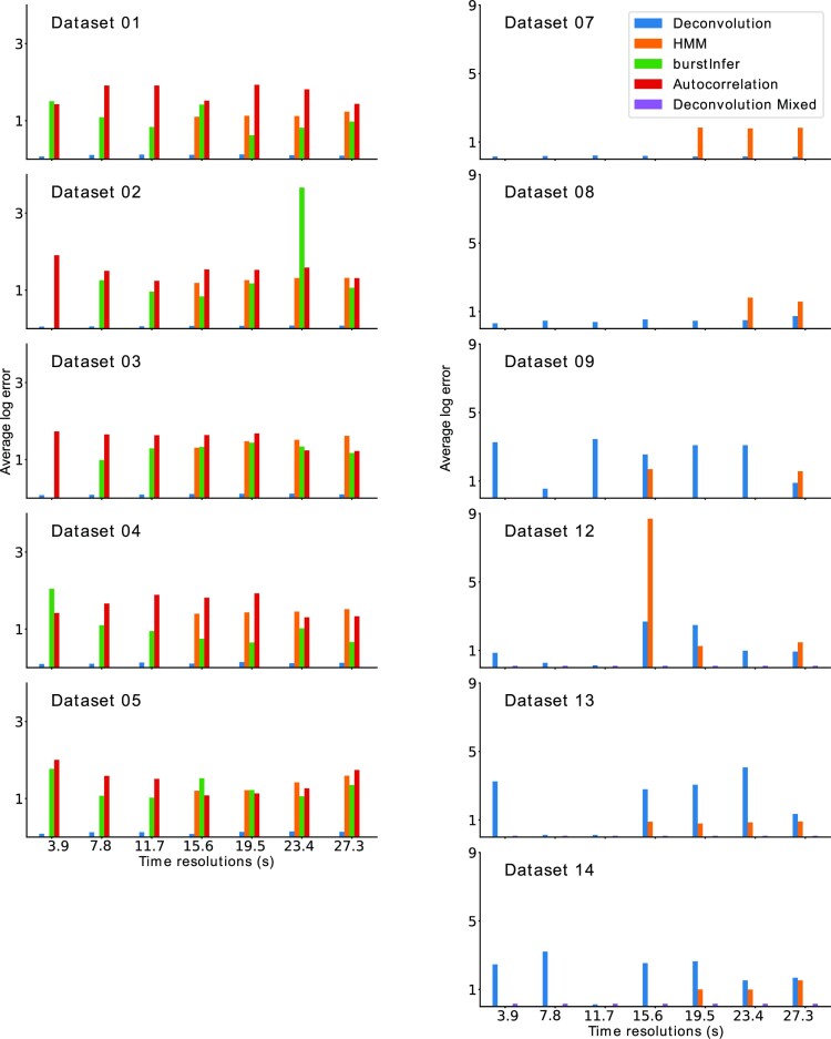
Given the difficulty of HMM in treating with high time resolutions, we have cross compared the kinetic parameter reconstruction error for several methods, using various artificial datasets and time resolutions. For the comparison we considered the two versions of BurstDECONV, the simple and the mixed one, using only short high resolution movies and both short and long movies, respectively. All the other methods were tested on short movies as they do not allow to combine movies of different time scales. All the artificial short movies last 26 min but their time resolution varies from 3.9 to 39 s. The HMM method was used in two versions: the ‘exact’ version implemented in (34) that explores the full state combinatorics of the promoter states and the ‘burstInfer’ version implemented in (36) that explores a reduced number of states. The auto-correlation method is represented by its implementation in (33). This implementation considers that the polymerase loading is deterministic with a known fixed rate (one polymerase every six seconds precisely, corresponding to our parameter k_ini = 0.166 s⁻¹) and fits only the switching rates of the random telegraph model (corresponding to our parameters k⁺ and k⁻). We have also tested inferring simultaneously all the parameters of the random telegraph model together with the polymerase dwell time using the auto-correlation method described in (32). In this case the parameters k⁺, k⁻ and k_ini can not be reliably reconstructed, but interestingly, we obtain stable estimates of the polymerase dwell time (see Materials and Methods and Supplementary Table S1).

The results of the method comparison in terms of accuracy are shown in Figure 9. They show that BurstDECONV is robust and can be applied to all the datasets and time resolutions. Because of combinatorial issues described above, HMM method may fail in some cases (by memory overflow or execution timeout).

Figure 9.

Parametric reconstruction accuracy of BurstDECONV vs. autocorrelation and HMM methods The bar plots on the left correspond to the parameter reconstruction errors for the four methods, BurstDECONV, cphmm, burstInfer (based on hmm) and Autocorrelation for datasets 1–5. These datasets correspond to a two state promoter model. The bar plots on the right depict the errors for BurstDECONV and for cphmm (datasets 7–9, 12–14 (3-state models)). BurstDECONV mixed refers to the deconvolution method combining high and low resolution movies. The x-axis for the plots have different time resolution of the short movies and the y-axis, the average log error (base 10). BurstDECONV mixed used short movies of resolution 3 s and long movies of resolution 3 min.

Whenever comparison was possible, for two-state datasets we found that the parameter reconstruction by BurstDECONV is significantly more accurate than by the other methods.

Some three-state datasets (D9,12–14) have very small switching rates (k⁺ or k⁻ or both). In this case, the precision of BurstDECONV is limited by the length of the short movie. Then, the simple deconvolution method can generate large errors and the ‘mixed’ version of BurstDECONV, that combines short and long movies, is needed. Interestingly, the HMM method seems to be slightly less sensitive to the same phenomenon. Although large, the estimation errors of HMM are smaller than those of the simple BurstDECONV, for datasets D13 and D14 (Figure 9). However, in such difficult cases, the ‘mixed’ version of BurstDECONV significantly supersedes in accuracy all the other methods.

Testing BurstDECONV using an enriched collection of datasets

The datasets of Table 1 span a large parameter range but the parametric resolution is poor. In order to increase this resolution, we generated more parameter sets by latin hypercube sampling.

We generated 40 more short movie synthetic datasets corresponding to two states models. The parameter values where defined by latin hypercube sampling in linear (20 datasets) and logarithmic (20 datasets) scales.

We also set up 240 more datasets for three states models. These correspond to 60 parameter sets obtained by latin hypercube sampling in linear (30 datasets) and logarithmic (30 datasets) scales. We doubled the number of parameter sets by including both M2 and M1 three state models with parameters corresponding to the same theoretical survival function. Finally, the three states datasets were produced in two versions, simple (short movie) and mixed (short and long movies).

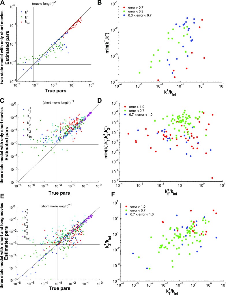
We have used BurstDECONV to reconstruct the parameters of these extra 280 synthetic datasets that add to those already presented in Table 1. The parameter values for these datasets can be found in the Supplementary Table S2. Figure 10 illustrates the result of these numerical experiments.

Figure 10.

Parametric reconstruction accuracy for an enriched collection of 297 synthetic datasets. (A) Estimated vs. true parameters for 45 datasets generated with two states models. (B) Error versus parameters (all 2-state datasets); the mean logarithmic error is large when k⁺ or k⁻ are small or when k⁺ is close to k_ini. (C) Estimated versus true parameters for three states models using the simple version of BurstDECONV. Only datasets with error <1 are shown (81 out of 126). (D) Error versus parameters (all 3-state datasets); similarly to 2-state models, the error is large for small or , i ∈ {1, 2}, or when or is close to k_ini. (E) Estimated versus true parameters for three states models using the mixed version of BurstDECONV. Only datasets with error <1 are shown (97 out of 126). (F) Error versus parameters (all 3-state datasets); the error is large when either or is close to k_ini.

The initiation rate parameter k_ini is accurately reconstructed for all models and datasets (Figure 10A and C). Indeed, this parameter scales inversely with the signal amplitude and is robust with respect to signal sampling. The lack of robustness of k_ini against calibration was illustrated in Figure 6C.

In contrast to k_ini, the switching parameters can be inaccurately reconstructed using the simple version of BurstDECONV. We have identified two main sources of error. First, the reconstruction error is large when the lifetimes of the ON and OFF states are larger than the movie duration or, equivalently, when k⁺ or k⁻ are smaller than the inverse of the short movie length. This effect is illustrated in Figure 10A–D. Second, when the lifetime of one of the OFF states becomes comparable to the interval between successive initiation events (1/k_ini) there is parametric uncertainty, as a model with less states fits equally well in this case. This effect, leading to large errors when or are large and close to k_ini is illustrated in Figure 10B, D, F.

As expected, the use of the mixed version of BurstDECONV (short and long movies) allows the reconstruction of very small switching parameters, corresponding to timescales larger than the length of the short movie (see Figure 10E). By using the mixed version, the error due to large lifetimes of ON and OFF states can be avoided.

DISCUSSION

While the development of imaging-based methods to monitor transcription in live cells and animals boomed over the last 20 years, the analytical frameworks extracting quantitative information from transcriptional bursting remained limited. Hence promoter switching was often modeled using ad hoc burst definitions, or using two states random telegraph model and rarely envisaging more complex models (18–20,39). Two main methods, namely the auto-correlation and the Hidden Markov Model (HMM) methods were employed in analysing transcriptional bursting data. However, there is no comparative benchmarking of the accuracy and robustness of these methods.

Here we provide BurstDECONV, a novel signal deconvolution method able to retrieve single polymerase initiation events from single cell transcription bursts and infer promoter states and their switching rates. We comparatively benchmark our method to the other two state of the art methods.

Our method is robust with respect to polymerase speed, signal calibration, time resolution, movie duration, and noise in the signal. The method is precise for wide values of kinetic parameters of the transcription regulation processes. By combining short and long movies, we are able to quantify processes with timescales from seconds to days. This extremely wide dynamic range was not accessible with the previous quantitative live cell transcription imaging approaches.

Thus, our method and tools are of interest in applications where a precise description of rate-limiting steps governing transcription dynamics is important: zygotic genome activation in model organisms, various aspects of gene expression regulation in human cells and tissues in health and disease, various studies of stochastic gene expression in prokaryotes and eukaryotes. Beyond transcription studies, they can be used for other applications where the signal can be deconvoluted into individual initiation events, for instance in studies of translation.

Another advantage of BurstDECONV resides in its ability to directly bridge agnostic representations of data to kinetic parameters of discrete state models of transcription. This is not possible in the framework of the HMM method, where each model has to be fitted separately using a different likelihood function. The survival function used in BurstDECONV conveys different information than the auto-correlation function used in previous methods. This renders the two methods complementary. BurstDECONV can not determine the polymerase dwell time, but provides accurate estimates of the transition rate parameters. The autocorrelation method can estimate the dwell time, but is imprecise on the transition rates.

BurstDECONV can be extended to consider more complex transcriptional bursting models, with arbitrary number of states and transition schemes, or with multiple non-resolvable active sites resulting, for instance, from sister chromatids.

In its current setting our method considers that transcription sites are statistically equivalent. This assumption is valid when there is limited spatial and temporal heterogeneity. However, a segmentation step could be easily added to the image analysis in order to select statistically equivalent sites in the case of spatial or temporal heterogeneity. This is the case in a multicellular organism, where gene expression is submitted to positional information like Drosophila patterning instructed by gradients of morphogens.

The output of BurstDECONV is a set of promoter states and the transition rates between these states. The quantitative framework proposed in this study reveals the key bottlenecks responsible for the promoter switching dynamics. Moreover, by informing on the timescale of each rate-limiting step, BurstDECONV provides a hint on the nature of these rate limiting steps. We foresee that with the development of novel perturbation methods (as for example optogenetics), the molecular characterization of these steps will be more and more facilitated.

In addition, our stochastic models of transcription dynamics can be readily used to test mechanistic hypotheses. For example, by applying BurstDECONV to two biological systems, HIV-1 transcription in Hela cells and zygotic transcription in Drosophila embryos, we came to the conclusion that a classical view of polymerase pausing may not be accurate. Indeed, a scenario where all polymerase would experience a discernable paused state was not compatible with our data. This analysis led us to propose a new view of pausing, a non-obligatory pausing model, where only a subset of polymerase would experience stable pausing, whereas other initiated polymerases would not be kinetically limited by such long pauses (19,20). Thus, monitoring transcription in live cells and employing rigorous analytical framework, could in some cases affect our classical view of the transcription process, often raised from biochemical in vitro and static approaches.

DATA AVAILABILITY

The artificial data as well as the code used for benchmarking the pipeline are available on Zenodo at https://zenodo.org/record/7438759. BurstDECONV source code is available in both MATLAB and Python 3 versions under 3-clause BSD open license. BurstDECONV is also available as a Graphical User Interface. The source codes are available through Github at https://github.com/oradules/BurstDECONV. For increased portability, we have created a Docker container for the Python notebook. Instructions for using this container can be found in the same Github repository. The GUI and the user manual are available on Zenodo at https://zenodo.org/record/7443044. BurstDECONV does not include the image analysis part of the pipeline. This can be performed with MS2-Quant https://bitbucket.org/muellerflorian/ms2_quant/src/master/ for cell line movies, segment-track https://github.com/ant-trullo/SegmentTrack_v4.0 for Drosophila movies, or with any other equivalent software.

SUPPLEMENTARY DATA

Supplementary Data are available at NAR Online.

FUNDING

Université de Montpellier; Centre National de la Recherche Scientifique, CNRS; European Research Council, ERC; Agence Nationale de Recherches sur le Sida et les Hépatites Virales, ANRS. Funding for open access charge: Université de Montpellier.

Conflict of interest statement. None declared.

REFERENCES

- 1. Bertrand E., Chartrand P., Schaefer M., Shenoy S.M., Singer R.H., Long R.M.. Localization of ASH1 mRNA particles in living yeast. Mol. Cell. 1998; 2:437–445. [DOI] [PubMed] [Google Scholar]
- 2. Chubb J.R., Trcek T., Shenoy S.M., Singer R.H.. Transcriptional pulsing of a developmental gene. Curr. biol. 2006; 16:1018–1025. [DOI] [PMC free article] [PubMed] [Google Scholar]
- 3. Ozbudak E.M., Thattai M., Kurtser I., Grossman A.D., Van Oudenaarden A.. Regulation of noise in the expression of a single gene. Nat. Genet. 2002; 31:69–73. [DOI] [PubMed] [Google Scholar]
- 4. Raser J.M., O’Shea E.K.. Control of stochasticity in eukaryotic gene expression. Science. 2004; 304:1811–1814. [DOI] [PMC free article] [PubMed] [Google Scholar]
- 5. Cai L., Friedman N., Xie X.S.. Stochastic protein expression in individual cells at the single molecule level. Nature. 2006; 440:358–362. [DOI] [PubMed] [Google Scholar]
- 6. Chong S., Chen C., Ge H., Xie X.S.. Mechanism of transcriptional bursting in bacteria. Cell. 2014; 158:314–326. [DOI] [PMC free article] [PubMed] [Google Scholar]
- 7. Nicolas D., Phillips N.E., Naef F.. What shapes eukaryotic transcriptional bursting. Mol. BioSyst. 2017; 13:1280–1290. [DOI] [PubMed] [Google Scholar]
- 8. Tunnacliffe E., Chubb J.R.. What is a transcriptional burst. Trends Genet. 2020; 36:288–297. [DOI] [PubMed] [Google Scholar]
- 9. Sanchez A., Garcia H.G., Jones D., Phillips R., Kondev J.. Effect of promoter architecture on the cell-to-cell variability in gene expression. PLoS Comput. Biol. 2011; 7:e1001100. [DOI] [PMC free article] [PubMed] [Google Scholar]
- 10. Sanchez A., Golding I.. Genetic determinants and cellular constraints in noisy gene expression. Science. 2013; 342:1188–1193. [DOI] [PMC free article] [PubMed] [Google Scholar]
- 11. Jones D.L., Brewster R.C., Phillips R.. Promoter architecture dictates cell-to-cell variability in gene expression. Science. 2014; 346:1533–1536. [DOI] [PMC free article] [PubMed] [Google Scholar]
- 12. Zoller B., Little S.C., Gregor T.. Diverse spatial expression patterns emerge from unified kinetics of transcriptional bursting. Cell. 2018; 175:835–847. [DOI] [PMC free article] [PubMed] [Google Scholar]
- 13. Bharucha-Reid A.T. Elements of the Theory of Markov Processes and their Applications. 1960; USA: McGraw-Hill Inc. [Google Scholar]
- 14. Peccoud J., Ycart B.. Markovian modeling of gene-product synthesis. Theor. Popul. Biol. 1995; 48:222–234. [Google Scholar]
- 15. Ferguson M.L., Le Coq D., Jules M., Aymerich S., Radulescu O., Declerck N., Royer C.A.. Reconciling molecular regulatory mechanisms with noise patterns of bacterial metabolic promoters in induced and repressed states. Proc. Natl. Acad. Sci. U.S.A. 2012; 109:155–160. [DOI] [PMC free article] [PubMed] [Google Scholar]
- 16. Lionnet T., Singer R.H.. Transcription goes digital. EMBO Rep. 2012; 13:313–321. [DOI] [PMC free article] [PubMed] [Google Scholar]
- 17. Suter D.M., Molina N., Gatfield D., Schneider K., Schibler U., Naef F.. Mammalian genes are transcribed with widely different bursting kinetics. Science. 2011; 332:472–474. [DOI] [PubMed] [Google Scholar]
- 18. Tantale K., Mueller F., Kozulic-Pirher A., Lesne A., Victor J.-M., Robert M.-C., Capozi S., Chouaib R., Bäcker V., Mateos-Langerak J.et al.. A single-molecule view of transcription reveals convoys of RNA polymerases and multi-scale bursting. Nat. Commun. 2016; 7:12248. [DOI] [PMC free article] [PubMed] [Google Scholar]
- 19. Tantale K., Garcia-Oliver E., Robert M.-C., L’Hostis A., Yang Y., Tsanov N., Topno R., Gostan T., Kozulic-Pirher A., Basu-Shrivastava M.et al.. Stochastic pausing at latent HIV-1 promoters generates transcriptional bursting. Nat. Commun. 2021; 12:4503. [DOI] [PMC free article] [PubMed] [Google Scholar]
- 20. Pimmett V.L., Dejean M., Fernandez C., Trullo A., Bertrand E., Radulescu O., Lagha M.. Quantitative imaging of transcription in living Drosophila embryos reveals the impact of core promoter motifs on promoter state dynamics. Nat. Commun. 2021; 12:4504. [DOI] [PMC free article] [PubMed] [Google Scholar]
- 21. Sánchez Á., Kondev J.. Transcriptional control of noise in gene expression. Proc. Natl. Acad. Sci. U.S.A. 2008; 105:5081–5086. [DOI] [PMC free article] [PubMed] [Google Scholar]
- 22. Innocentini G. d. C.P., Forger M., Ramos A.F., Radulescu O., Hornos J.E.M.. Multimodality and flexibility of stochastic gene expression. Bull. Math. Biol. 2013; 75:2600–2630. [DOI] [PubMed] [Google Scholar]
- 23. Vos S.M., Farnung L., Urlaub H., Cramer P.. Structure of paused transcription complex Pol II–DSIF–NELF. Nature. 2018; 560:601–606. [DOI] [PMC free article] [PubMed] [Google Scholar]
- 24. Vos S.M., Farnung L., Boehning M., Wigge C., Linden A., Urlaub H., Cramer P.. Structure of activated transcription complex Pol II–DSIF–PAF–SPT6. Nature. 2018; 560:607–612. [DOI] [PubMed] [Google Scholar]
- 25. Rodriguez J., Larson D.R.. Transcription in living cells: molecular mechanisms of bursting. Annu. Rev. Biochem. 2020; 89:189–212. [DOI] [PubMed] [Google Scholar]
- 26. Krebs A.R., Imanci D., Hoerner L., Gaidatzis D., Burger L., Schübeler D.. Genome-wide single-molecule footprinting reveals high RNA polymerase II turnover at paused promoters. Mol. Cell. 2017; 67:411–422. [DOI] [PMC free article] [PubMed] [Google Scholar]
- 27. Roeder R.G. 50+ years of eukaryotic transcription: an expanding universe of factors and mechanisms. Nat. Struct. Mol. Biol. 2019; 26:783–791. [DOI] [PMC free article] [PubMed] [Google Scholar]
- 28. Osman S., Cramer P.. Structural biology of RNA polymerase II transcription: 20 years on. Annu. Rev. Cell Dev. Biol. 2020; 36:1–34. [DOI] [PubMed] [Google Scholar]
- 29. Patel A.B., Greber B.J., Nogales E.. Recent insights into the structure of TFIID, its assembly, and its binding to core promoter. Curr. Opin. Struct. Biol. 2020; 61:17–24. [DOI] [PMC free article] [PubMed] [Google Scholar]
- 30. Rengachari S., Schilbach S., Aibara S., Dienemann C., Cramer P.. Structure of the human Mediator–RNA polymerase II pre-initiation complex. Nature. 2021; 594:129–133. [DOI] [PubMed] [Google Scholar]
- 31. Fianu I., Chen Y., Dienemann C., Dybkov O., Linden A., Urlaub H., Cramer P.. Structural basis of Integrator-mediated transcription regulation. Science. 2021; 374:883–887. [DOI] [PubMed] [Google Scholar]
- 32. Coulon A., Larson D.R.. Fluctuation analysis: dissecting transcriptional kinetics with signal theory. Methods in enzymology. 2016; 572:Elsevier; 159–191. [DOI] [PMC free article] [PubMed] [Google Scholar]
- 33. Desponds J., Tran H., Ferraro T., Lucas T., Romero C.P., Guillou A., Fradin C., Coppey M., Dostatni N., Walczak A.M.. Precision of readout at the hunchback gene: analyzing short transcription time traces in living fly embryos. PLoS Comput. Biol. 2016; 12:e1005256. [DOI] [PMC free article] [PubMed] [Google Scholar]
- 34. Lammers N.C., Galstyan V., Reimer A., Medin S.A., Wiggins C.H., Garcia H.G.. Multimodal transcriptional control of pattern formation in embryonic development. Proc. Natl. Acad. Sci. U.S.A. 2020; 117:836–847. [DOI] [PMC free article] [PubMed] [Google Scholar]
- 35. Lammers N.C., Kim Y.J., Zhao J., Garcia H.G.. A matter of time: using dynamics and theory to uncover mechanisms of transcriptional bursting. Curr. Opin. Cell Biol. 2020; 67:147–157. [DOI] [PMC free article] [PubMed] [Google Scholar]
- 36. Bowles J.R., Hoppe, C., Ashe, H.L., Rattray M.. Scalable inference of transcriptional kinetic parameters from MS2 time series data. Bioinformatics (Oxford, England). 2021; 38:1030–1036. [DOI] [PMC free article] [PubMed] [Google Scholar]
- 37. Hougaard P. Analysis of Multivariate Survival Data. 2000; 564:Springer. [Google Scholar]
- 38. Pichon X., Lagha M., Mueller F., Bertrand E.. A growing toolbox to image gene expression in single cells: sensitive approaches for demanding challenges. Mol. Cell. 2018; 71:468–480. [DOI] [PubMed] [Google Scholar]
- 39. Corrigan A.M., Tunnacliffe E., Cannon D., Chubb J.R.. A continuum model of transcriptional bursting. Elife. 2016; 5:e13051. [DOI] [PMC free article] [PubMed] [Google Scholar]
- 40. Wissink E.M., Vihervaara A., Tippens N.D., Lis J.T.. Nascent RNA analyses: tracking transcription and its regulation. Nat. Rev. Genet. 2019; 20:705–723. [DOI] [PMC free article] [PubMed] [Google Scholar]
- 41. Liu Y. Non-Parametric Bayesian Inference with Application to System Biology. 2022; Department of Statistics, University of Chicago; PhD thesis. [Google Scholar]
- 42. Ferguson M.L., Larson D.R.. Measuring transcription dynamics in living cells using fluctuation analysis. Imaging Gene Expression. 2013; Springer; 47–60. [DOI] [PMC free article] [PubMed] [Google Scholar]
Associated Data
This section collects any data citations, data availability statements, or supplementary materials included in this article.
Supplementary Materials
Data Availability Statement