

Abstract
Acoustoelectric imaging (AEI) is a technique that combines ultrasound with radiofrequency recording to detect and map local current source densities. This study demonstrates a new method called Acoustoelectric Time Reversal (AETR), which uses AEI of a small current source to correct for phase aberrations through a skull or other ultrasound-aberrating layers with applications to brain imaging and therapy. Simulations conducted at three different US frequencies (0.5, 1.5 and 2.5 MHz) were performed through media layered with different sound speeds and geometries to induce aberrations of the US beam. Time delays of the acoustoelectric signal from a monopole within the medium was calculated for each element to enable corrections using AETR. Uncorrected aberrated beam profiles were compared with those after applying AETR corrections, which demonstrated a strong recovery (29–100%) of lateral resolution and increases in focal pressure up to 283%. To further demonstrate the practical feasibility of AETR, we further conducted bench-top experiments using a 2.5 MHz linear US array to perform AETR through 3D-printed aberrating objects. These experiments restored lost lateral restoration up to 100% for the different aberrators and increased focal pressure up to 230% after applying AETR corrections. Cumulatively, these results highlight AETR as a powerful tool for correcting focal aberrations in the presence of a local current source with applications to AEI, ultrasound imaging, neuromodulation, and therapy.
Keywords: Transcranial brain imaging, ultrasound neuromodulation, HIFU, time reversal, skull aberrations
I. INTRODUCTION
Optimal ultrasound (US) focusing through the skull is critical for applications in ultrasound imaging1–3, neuromodulation4–6, and therapy.7–10 Phase aberrations through bone and other materials lead to detriments in beam accuracy, resolution and focal pressure.11 Several methods have been developed to correct for ultrasound aberrations and fall into two distinct categories: imaging-based and point-target based corrections.
Imaging-based aberration correction uses size, surface morphology and density information about the skull gained from either magnetic resonance imaging (MRI) or x-ray computed tomography (CT).8,12,13 Transcranial US models14 with neuronavigation combines this information with estimates of sound-speed to output optimized delay profiles to focus more accurately through the skull to target locations.15–19 This method is both popular and effective in low frequency applications like high intensity focused ultrasound ablation (HIFU).20,21 However, as the US frequency increases, the attenuation and aberration induced by the skull layers also increases, demanding higher levels of property estimation for accurate beam correction, which ultimately limits the viability of this technique. Because of these and other factors, imaging-based correction remains challenging.
Point-target based aberration correction, on the other hand, uses points within the object of interest (i.e., the brain) to act as a scatterer, emitter, or receiver of a pulsed US wave. By measuring the time-of-flight (ToF) between a wave propagating between each element of an US phased-array and the point target, an optimal set of delays can be acquired to produce a focused beam at that location. Several algorithms have been developed to leverage this form of correction via sparse point scatterers.22–25 Expansion of these methods enabled the inclusion of extended reflectors26 and multiple scatters27 or multiple foci from one scatterer28. However, given the lack of native scatterers in the brain, time-reversal (TR) methods remained largely impractical until the introduction of alien scatterers such as microbubbles,29,30 droplet vaporization,31 and cavitation.32,33 Even with these developments, TR methods for transcranial US phase-aberration correction remain limited with clinical transcranial Doppler imaging and other applications opting to bypass corrections altogether.34
This study, on the other hand, describes a new method called acoustoelectric time reversal (AETR) for correcting US aberrations through the skull and other materials. AETR takes advantage of the acoustoelectric (AE) effect and Ohms law to calculate time delays as an ultrasound beam interacts with a local current source (e.g., monopole).35–38 The AE effect describes a modulation of resistivity as an acoustic wave propagates through a material; in the presence of a local current, Ohm’s law also applies such that a voltage signal is detectable across a pair of recording electrodes as the ultrasound pulse arrives at the target.39 This approach has been used in acoustoelectric imaging (AEI), which has opened the door to non-invasive mapping of current source densities from brain currents40,41 and those produced artificially by a deep brain stimulator.42–44 This modality has also been effective in imaging cardiac activation currents from the isolated rabbit heart45,46 and, more recently, in vivo swine heart.47,48 Instead of imaging physiologic currents, this study describes how this mechanism may be used to correct for phase delays of the US beam through aberrating materials in scenarios where a subject potentially has a suitable current source as a target, such as a contact on a deep brain stimulator or other implantable device.49–51 The objective, therefore, is to 1) use simulations to assess the practicality and efficacy of AETR to correct for phase aberrations through different shaped aberrators and 2) demonstrate proof-of-concept in benchtop AETR experiments at a common transcranial US imaging frequency of 2.5MHz.52–55 Finally, we discuss possible clinical scenarios where this technique may be useful for optimizing US focusing through the skull.
II. METHODS
2.1. Acoustoelectric Theory
AEI is capable of 4D volumetric imaging of time-varying electrical currents based on the general AE equation:
| (1) |
where is the detected AE signal, is a material specific AE constant56, is the projection of the current densities and lead field of the recording electrodes, is initial resistivity of the material, is change in pressure induced by the propagating pulsed US wave, is time associated with the propagation of the US wave, is time associated with the electrical current, and and denote US beam position in the lateral and elevational directions. Full derivations of this equation have been performed elsewhere39. It is important to note that and typically vary by at least 3 orders of magnitude, with operating in milliseconds and in microseconds.
In the case where the US transmit pulse is stationary, Equation 1 reduces to one-dimension:
| (2) |
Moreover, the scaling effects of the lead field are negligible when recording across a single pair of far field electrodes with the assumption that differences in material resistivity surrounding the current source is also negligible, such as in a saline bath, Equation 2 further reduces to:
| (3) |
which simply represents the convolution of the current source by the propagating US wave.
2.2. Acoustoelectric Time Reversal
Focused US functions by matching the time of flight (ToF) of the propagation of pulsed waves from each element on an US transducer to a desired target. That is, the delay, , of element is the latency in time between the firing of an element and its detected interaction at some current source. Given a uniform sound speed medium, this can simply be represented as the hypotenuse between the two points as depicted by the thin black arrow in Fig 1A and represented by (4):
| (4) |
where is the sound speed of medium and and represent the horizontal and vertical displacements from the current source of element , respectively. Moreover, if the medium is non-uniform but the size and sound speed of each varying sector is known, the latencies can still be determined by weighting according to (4) to the average sound speed of each US elements unique path to the target. However, when the average cannot be estimated a priori, then optimal delays per element cannot be computed. TR rectifies this problem by calculating the latency between each US element and the target experimentally. Cross-correlation is used between the recorded AE signals generated independently by each element, , with the recorded waveform of an arbitrarily chosen element, , as described in (5):
| (5) |
where the function represents the time-to-rectified-peak of its argument. The normalized relative delays, , are then found by subtracting by its largest value and taking the absolute value of the result, as shown in (6), such that the elements furthest in time from the target fire earliest.
| (6) |
Figure 1:

(A) Schematic of acoustoelectric time reversal (AETR) with one element emitting a spherical US pulse to measure the time of flight (ToF) between it and an electrical target. (B) Representative AE signal detected for one of the elements during the delay acquisition process. (C) The detected AE signal over depth for each of the 96 elements on the US transducer. (D) Normalized magnitude of , the cross-correlation function between the AE signal of one element and that of the template element, . (E) Profile of time-reversed differences per element relative to the element with shortest latency (e.g., from wedge aberrator).
2.3. Simulations
The acoustic simulations leveraged the k-Wave package for MATLAB (Mathworks, Natick, MA, USA).14,57 The simulated environment contained 400×400 pixels with 0.1mm pixel size (lateral) and 0.15 mm size (depth) to produce a 40 × 60 mm domain. The pixel density was a compromise between computation time and accuracy, since k-space methods retain high levels of accuracy even at 2 grid points per wavelength.58
The simulated US transducer was composed of 96 independent acoustic sources similar to another simulation study on transcranial US.59 Each element was excited to emit a 3-cycle Gaussian-enveloped sinusoidal pulse centered at 0.5, 1.5, or 2.5 MHz. The delay to the onset of the pulse was independently controlled for each element. The 96 element US-transducer spanned 2.88 cm in the lateral dimension with widths of 0.2 mm and inter-element spacing of 0.1 mm. The propagation of the simulated acoustic waves occurred over 1400 time points with . The location of each element in the linear array is depicted in Fig 2Aii as yellow rectangles.
Figure 2:

A and B) The three-layered media used during simulation, as well as the density (A) and sound speed (B) values for the water, skull, and brain layers. Image Aii also depicts the location of the US transducer elements in yellow and focus in red. C) Simulation outputs for (i) the pressure waveform of a 2.5 MHz beam, (ii) the static current and (iii) the recorded AE signal generated by their interaction. To include dispersion, the alpha power used for all layers was 1.2.
The simulated media varied in and material density, using properties of water, skull, and brain. While human skull properties can vary largely between sections, layers and individual subjects, these numbers represent the average values taken from multiple transcranial US studies.3,44,60,61 The values and locations of each layer are shown in Fig 2Ai and 2Bi. Additionally, Fig 2 depicts the full media for 3 of the 4 of the simulated conditions, giving the shapes of the three aberrating layers we used – plate, concave lens and pseudo-skull (a non-uniform, slightly curved layer). A fourth, control, simulation medium was also used, which was uniform with and density values for the brain only. The simulations were run in a noiseless environment and only the loss of signal integrity due to reflection and refraction (as opposed to attenuation) was considered. This environment was chosen to explore the efficacy of AETR under imaging conditions with sufficient signal-to-noise ratio (SNR).
A static two-dimensional current density was also simulated in MATLAB. The current source (an ideal monopole) was centered at the focal point of the US transducer (x in Fig. 2Aii) assuming homogenous media of brain sound-speed. This was done as a simplification since, as previously noted, static inhomogeneities in sound-speed do not impact the effectiveness of TR algorithms. The size of the monopole was generated from a 0.2 × 02 mm source of charge . The electric field, , from the charge was computed as:
| (7) |
where is the permittivity and is the distance from the source charge. For simplicity, and were set to and and for all to normalize peak electric field to 1. This was then converted to a current density, as:
| (8) |
where is the electrical resistivity of the medium set uniformly to since the amplitude of the current in a noiseless system is arbitrary and the current spread outside of the simulated brain region was negligible. Likewise, the scaling factors in Eq. 3, and , were both uniformly set to 1 such that the computed AE signal was simply the sum of the dot product over time of the static current with the traveling pressure wave represented in Equation 9:
| (9) |
where and are 400×400 and 400×400×1400 matrices, respectively, and the wave in travels at sound-speed at iterations . Fig 2C illustrates examples of the time-varying pressure matrix, static current matrix, and resulting AE signal.
2.4. Bench-top Experiments
We constructed a benchtop setup as illustrated in Figure 3 to compare with simulation results. A 96-element commercial linear array transducer centered at 2.5 MHz (P4–1, Philips, Amsterdam, Netherlands) was used similar to the simulations. The US transducer was controlled by a commercial US system (Vantage 64LE, Verasonics, Kirkland, WA, USA). The aberrators were developed in SOLIDWORKS™ (Dassault Systemes, Velizy-Villacoublay, France) and 3D printed using VeroBlack (StrataSys, Eden Prairie, MN, USA) material with density , sound speed , and attenuation coefficient at 2.5 MHz. This material was chosen for its similar sound-speed properties to skull, but lower density and attenuation.3,60 The aberrators were attached to the US array by inserting them into a waveguide extending from the US transducer (Fig 3A). The aberrators tested were a 0.3 mm plate, 0.7 mm plate, concave lens, convex lens, wedge, and a sinusoidal-like block.
Figure 3:
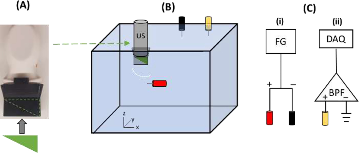
A) Photograph of the 96 element 2.5 MHz US transducer with custom 3D-printed waveguide used in the study. The aberrators were inserted into the waveguide. B) Cartoon of the experimental setup. The US probe was positioned over the anode (red) with different aberrators inserted between the two (wedge depicted) and representation of a spherical wave emitted from a single element after passing through the wedge aberrator. The black and yellow electrodes represent cathode and recording electrodes. C) Connection diagram for stimulation (i) and recording AE signals (ii). FG = function generator, DAQ = data acquisition, BPF = bandpass filter.
To perform AETR and generate AE signals, a platinum current source electrode was inserted into a tank of water containing 0.9% NaCl to mimic the physiological conductivity of the brain. The tip of the US transducer was submerged above the current source electrode. The current sink was introduced using an additional platinum electrode and positioned at the edge of the tank to generate a monopole within the functional field of view of the US transducer. Another separate tungsten electrode was inserted into the tank to record the voltage and acquire the AE signal. The recorded voltage was passed through a differential amplifier (referenced to ground) and bandpass filtered between 0.2 and 5 MHz to remove the low frequency content and isolate the AE signal near the carrier frequency of the US waves (centered at 2.5 MHz). The signal was then digitized at 20 MHz (NI PXI-5105, National Instruments, Austin, TX, USA).
The input current was generated as a three-cycle 200Hz sine wave at 6V (pk-pk) using a function generator (33220A, Agilent, Santa Clara, CA, USA). A sine wave was chosen due to its simplicity in filtering, and the frequency was chosen to slightly exceed the normal ranges of both evoked neural activity and DBS pulse repetition frequencies. The US waveform was a pulsed 20 cycle chirp encompassing the full bandwidth of the US transducer (1–4 MHz) at 6 kHz pulse repetition frequency. The chirp encoding was used to increase the signal-to-noise ratio (SNR) of the AE signal.62 After digitization, the AE signal was further filtered using a matched filter to the output chirp waveform to compress the signal, improve SNR, and restore spatial resolution.62 The time waveform of the input current remained arbitrary for this experiment insofar as it was periodic, since only the time that generated the peak AE signal was used for the AETR process.
2.5. Assessing AETR efficacy
Assessing the efficacy of AETR was approached differently for the simulations than the experiments. For simulations, the pressure waveforms themselves were analyzed. Comparisons between trials (control vs. uncorrected vs AETR corrected) were made using the envelope pressure images at the time when there was peak pressure at the center location of the current source used during AETR, which were at approximately the same location as the designed focal point for the uncorrected/control delays). Therefore, only the AETR delays acquired at that one desired focal point were necessary for a full analysis. For the experimental analysis, on the other hand, the AE signal was used since direct pressure measurements in the region of interest would not be obtainable in any practical application for AETR. “Control” data represented the ideal beam pattern with the current source placed in water (without the abberrator) at approximately the same depth and lateral location as the “uncorrected” and “AETR corrected” test cases. For both the uncorrected and AETR corrected trials, full sets of delays were needed for all focal points along the lateral axis to generate 2D images. We used a of 0.25mm and a range of 10 mm in the lateral dimension for each scan; thus, 41 different sets of delays were necessary to create 2D AE-B-mode images for analysis. A template was created using a single set of AETR delays for centered focus by subtracting it from the uncorrected delays for centered focus.63 This template was then added to the uncorrected delays for the other 40 lateral positions to generate corrected delays for all 41 delay structures as displayed in Fig 4. Importantly, this focusing method is only valid for small angles, such as those used here.
Figure 4:

(A) Standard geometric and (B) AETR-derived delay profiles in s for the 96 elements when focusing to z = 45 mm at 41 equally spaced lateral positions between −5 and 5 mm. Each line represents a different lateral focal position.
III. Results
3.1. Simulations
Figs. 5–7 present the envelopes of each simulated pressure field along with the element delays and lateral plots through the focus for the 2.5, 1.5 and 0.5 MHz simulations, respectively. At all three frequencies, control trials (without an aberrator) showed nearly identical delay profiles and resulting pressure profiles for the uncorrected (black line) versus AETR (red hash). With the aberrators, however, the 2.5 MHz trials received the largest aberrations, while the 0.5 MHz trials received the least. This can be visualized as a percent change between the uncorrected and AETR trials for all frequencies and conditions plotted in Fig. 8. The major characteristics (shape and relative delays) of the AETR delay profiles, on the other hand, were mostly consistent among all frequencies and primarily dependent on the shape of the aberrator.
Figure 5:

Simulation results for each aberrator using a 2.5 MHz US transducer. A) Delay profiles for each medium. Solid black line indicates uncorrected delays calculated for homogenous brain media; red-hashed line indicates corrected delays from AETR. B) and C) Resulting pressure envelopes at the focal point when using the uncorrected (B) or AETR corrected (C) delays. D) Plots of the lateral beam profiles through the focal point for the uncorrected (solid black) and AETR corrected (red-hashed) delay profiles.
Figure 7:

Simulation results for each aberrator using a 0.5 MHz US transducer. A) Delay profiles used for each medium. Solid black line indicates uncorrected delays calculated for homogenous brain media; red-hashed line indicates corrected delays from AETR and the resulting pressure envelopes at the focal point when using the uncorrected (B) and AETR corrected (C) delays. D) Lateral beam profile plots through the focal point for the uncorrected (solid black) and AETR corrected (red-hashed) delay profiles.
Figure 8:

Improvement to image quality after AETR for each aberrating condition and US frequency expressed as percent. # within bar denotes actual improvement, if >200%.
Focusing through the 0.9mm plate resulted in AETR delay profiles of flattened (lower maximum delay) parabolas compared to the uncorrected focus. At 2.5 MHz, there was a notable increase in peak pressure of 35% at the focal point for the AETR trial compared to uncorrected. This effect lessened as the US frequency decreased, resulting in gains of only 15% and 2% for 1.5 and 0.5 MHz respectively. Similarly, when correcting delays through AETR, lateral FWHMs through the foci exhibited percent decreases of 20%, 5% and 0% at 2.5, 1.5 and 0.5 MHz, respectively. Lastly, the axial FWHMs remained unchanged, with percent decreases of only ~1% at each frequency.
The concave lens aberrator, on the other hand, induced much larger wave aberrations. As a result, the AETR delay profiles were significantly flattened, with peak relative delays of only (compared to when uncorrected). The distal elements of the US transducer received parabolically increased average sound speed due to the thicker skull layer at those locations, resulting in a wavefront that converged before the target location. Thus, the wavefront had begun diverging before the wavefront reached the target. This divergence in focus can be seen as multiple peaks in the lateral profile of the pressure envelopes of the 2.5 and 1.5 MHz trials. At 0.5 MHz, the beam did not fully diverge at the intended focal point, but the initiation of divergence led to a wider, more triangular lateral profile. However, despite the variability in degree of aberration at each US frequency, in all cases, AETR reduced the aberrations and resulted in focused beam profiles similar to the controls and nearly identical to those acquired through the corrected plate. Axial FWHMs were more largely and variably impacted by the concave aberrator than the plate, but these effects still dwarfed in comparison to the loss in lateral resolution and peak pressure.
Lastly, the asymmetrical pseudo-skull layer induced both defocusing as well as refraction. As a result, the uncorrected pressure envelopes not only widened, but also defocused along the lateral axis (from 0 – 1.5 mm). The corresponding AETR delay profiles lose their symmetrically parabolic shapes. By applying these AETR delays, both sources of aberrations were corrected, refocusing the beam on the lateral axis while also addressing the depth of focus.
Tables 1–3 contain the metrics (peak envelope pressure, lateral FWHM and axial FWHM) for each aberrator at each frequency. Fig. 8 illustrates the percent improvement for each metric after AETR. In summary, the simulations revealed that aberrators induced defocusing through changes in sound speed, but in all cases refocusing was possible through AETR.
Table 1:
Simulation results at 2.5MHz
| 2.5 MHz Simulation | ||||||
|---|---|---|---|---|---|---|
| Peak (Pa) | Lateral FWHM (mm) | Axial FWHM (mm) | ||||
| Aberrator | Uncorrected | AETR | Uncorrected | AETR | Uncorrected | AETR |
| Control | 4.69 | 4.64 | 1.32 | 1.32 | 0.825 | 0.84 |
| Plate | 1.90 | 2.57 | 2.02 | 1.62 | 1.55 | 1.54 |
| Concave | 0.960 | 2.72 | 8.96 | 1.3 | 2.01 | 1.69 |
| Pseudo | 1.67 | 2.53 | 3.91 | 1.51 | 2.19 | 1.53 |
Table 3:
Simulation results at 0.5MHz
| 0.5 MHz Simulation | ||||||
|---|---|---|---|---|---|---|
| Peak (Pa) | Lateral FWHM (mm) | Axial FWHM (mm) | ||||
| Aberrator | Uncorrected | AETR | Uncorrected | AETR | Uncorrected | AETR |
| Control | 7.75 | 7.75 | 5.38 | 5.38 | 3.71 | 3.71 |
| Plate | 4.69 | 4.77 | 6.28 | 6.31 | 3.74 | 3.72 |
| Concave | 3.88 | 5.27 | 7.43 | 5.14 | 3.75 | 3.71 |
| Pseudo | 4.91 | 5.02 | 6.03 | 5.9 | 3.75 | 3.73 |
3.2. Bench-top Experiments
The experimental results follow the same trajectory as the simulations with three major differences: 1) only a 2.5 MHz US transducer was tested; 2) each aberrator has its own control condition due to minor (mm scale) variability in placement of the electrode relative to the US transducer during each trial; and 3) comparative metrics were taken from resulting AE signals rather than directly detecting the pressure fields with a hydrophone. The AE envelopes for each trial (control, uncorrected, AETR) of the six different aberrators are depicted in Fig. 9 with corresponding AETR delay profiles in Fig. 10. The quantitative metrics are displayed in Table 4, and the % improvement of AETR is graphed in Fig. 11.
Figure 9:

AE B-Mode images from a monopole generated by the needle electrode. Each column contains the images from a different aberrator indicated at the top of each column. Each row relates to a different focusing condition with the “control” representing the image of the current source placed at a similar location in space in water without the abberrator. Green scale bars in top left image denote 2 mm.
Figure 10:

AETR delay profiles calculated for each aberrator.
Table 4:
Bench-top experimental results. Uncorr = uncorrected trial
| Normalized Peak Amplitude | Lateral FWHM (mm) | Axial FWHM (mm) | |||||||
|---|---|---|---|---|---|---|---|---|---|
| Control | Uncorr | AETR | Control | Uncorr | AETR | Control | Uncorr | AETR | |
| 3mm Plate | 1.00 | 0.712 | 0.710 | 2.00 | 2.25 | 2.00 | 0.917 | 0.978 | 0.978 |
| 7mm Plate | 1.00 | 0.448 | 0.601 | 2.00 | 2.75 | 2.00 | 0.917 | 0.978 | 1.04 |
| Convex | 1.00 | 0.525 | 0.545 | 2.00 | 2.00 | 2.00 | 0.978 | 0.978 | 1.04 |
| Wedge | 1.00 | 0.515 | 0.500 | 2.00 | 2.00 | 2.00 | 0.917 | 1.04 | 0.979 |
| Concave | 1.00 | 0.370 | 0.863 | 2.00 | 7.75 | 1.75 | 0.917 | 0.978 | 0.917 |
| Sine | 1.00 | 0.328 | 0.603 | 2.00 | 6.50 | 2.00 | 1.04 | 1.04 | 1.04 |
Figure 11:

Experimental improvement in imaging metrics after AETR for each aberrator at 2.5MHz.
As with the simulations, the two plates (0.3 and 0.7 mm thick) had only a minor impact on the resulting pressure field and AE signals. Notably, the thicker plate more heavily attenuated the acoustic pressure, and the increased axial defocusing resulted in a larger lateral FWHM (2.75 vs 2.25 mm), compared to the thinner plate. After correction with the AETR delays, however, the lateral FWHMs returned to control values (2.0 mm). Additionally, the AE signal amplitude increased from 45% to 60% that of control for the thicker plate. The thinner plate saw no increase in signal amplitude after correction.
The convex aberrator also had only a minor impact on the AE signal. Interestingly, however, there was also minor lateral refocusing of the beam by ~1 mm in the uncorrected trial, which may have been the result of an incomplete fitting of the aberrator against the face of the US transducer. In any case, it can be seen from the recentering of the AE envelope on the lateral axis in the AETR trial that this defocusing was corrected using the AETR delays. However, there was no noticeable increase in peak AE signal amplitude after applying AETR. Also, the lateral FWHM remained at 2.0 mm for the control and both conditions.
The wedge aberrator induced both depth and lateral defocusing of the beam resulting in a perceived signal 2 mm shallower and 5 mm off the lateral axis. After applying AETR, the lateral displacement induced by the wedge was corrected, resulting in a centered AE signal. As with the convex aberrator, the wedge did not noticeably impact the lateral FWHM of the US beam, thus all conditions remained at 2.0 mm. Additionally there was no increment in the AE signal peak after AETR (52% vs 50% compared to control for uncorrected and AETR, respectively).
The concave block resulted in large aberrations to both peak AE signals (decreased to 37%) and lateral FWHM (increased to 7.75 mm). Refocusing with AETR managed to significantly correct these aberrations, returning peak AE signal to 86% and lateral FWHM to 1.8 mm, similar to the control (2.0 mm).
Finally, the sinusoidal-like block produced strong aberrations in the AE signal. Notably, it decentered and split the beam into two foci, resulting in the illusory appearance of two current sources in the AE envelope image. The corresponding AETR delay profile in Fig. 10 exhibits the asymmetrical clustering of elements along each side of the US transducer with a sharp transition at the inflection point of the sinusoidal-like block. As seen in Fig. 9, applying the AETR derived delay profile managed to correct for these aberrations, returning the signal shape very similar to that of the control. In quantification, correcting for the aberration restored the peak AE signal from 33% to 60% that of the control amplitude and restored the lateral FWHM from 6.50 mm (taken from the more centered signal) back to the control (2.00 mm). Although there were no significant changes to the axial FWHM in any conditions, the values are reported in Table 4.
IV. Discussion
This study described aberration correction through different shaped materials using AETR in both simulations and bench-top experiments. In all cases, AETR matched or outperformed uncorrected beamforming in both peak amplitude and lateral resolution. The performance was similar to other TR-based studies,32,59 including a simplified simulation study comparing AETR with TR from a point hydrophone detector.64 These results collectively showcase the potential of using a localized current source and remote detection of the AE signal for TR phase aberration correction.
We envision possible clinical and basic research scenarios where this technique may prove valuable whenever there is a local current source that can be used as a target for AETR. Approximately 12,000 people receive chronic DBS implants each year for treatment of Parkinson’s disease, essential tremor and other conditions. Thousands of other subjects receive implantable electrodes for acute stimulation and extraoperative monitoring to help identify seizure foci and critical brain regions vital to survival prior to surgical intervention. In these situations, one or more contacts may be used to produce a small transient current to perform AETR to optimize focusing of an US beam through the skull to study, for example, mechanisms of ultrasound neuromodulation or develop strategies for improving focused ultrasound therapy. Aberration correction techniques like AETR can also be used together with other methods, such as MR thermometry40, MR acoustic radiation force41, and stereotactic navigation to improve the accuracy of directing a beam to a target location. Since AETR can be performed outside the surgical suite or MRI scanner, the technique could be employed extraoperatively or in a research setting. In preclinical studies of focused ultrasound therapy or neuromodulation, a small contact or microwire could be inserted near the region of interest to help locate and calibrate the US beam without the need for MR guidance or feedback. AETR would be most useful in large animal studies, such as swine and non-human primates, where skull thickness would otherwise cause significant US beam distortion.
In addition, AETR could be used to minimize aberrations for transcranial AE imaging of neuronal or stimulation currents near implanted electrode contacts. We have previously demonstrated transcranial acoustoelectric imaging (tAEI) for real-time mapping of stimulation currents near contacts on clinical devices42–46,68 and, most recently, using a neuronavigation system with MRI guidance for US targeting.69 tAEI with AETR for beam optimization could provide valuable feedback during surgical placement of DBS devices by producing high resolution, real-time feedback during implantation. It is well known that accurate lead placement for treatment of essential tremor is critical for ensuring effective, long-term treatment in patients.51–53 Similarly, when either verifying placement integrity post-surgery51,52 or when mapping the spread of current from the DBS leads into the brain,46,68 future studies that include AETR for aberration correction would improve the quality (resolution, sensitivity, and accuracy) of tAEI.
Transcranial acoustoelectric brain imaging (tABI) with aberration correction could also promote accurate electrical brain mapping of time-locked neuronal currents and neural activation patterns associated with behavior, such as facial recognition79,80 or distinct finger sensation81,82. Compared to fMRI and scalp EEG, tABI as a new modality directly measures functional brain signals at the mm and ms scales directly proportional to local currents.77,81–85 A recent study in acoustoelectric cardiac imaging further demonstrated feasibility and sufficient sensitivity for in vivo detection of bioelectric signals in the heart.49–50
One limitation in this study was the relatively weak detection of the AE signal. Previously reported experiments using the same or similar types of US arrays suggest a detection threshold of less than 0.5 mA at 1 MPa peak pressure.42,46,69 Unlike these other studies that exploited the full transmit aperture of the US array, this study was limited by single-element transmission of a phased array with peak negative pressures on the order of 0.15 MPa (or MI=0.1), which is well below safety guidelines determined by the FDA for diagnostic US imaging.69 Because our experiments used larger peak currents within range of DBS (<5 mA), we were able to compensate for the weaker pressures and still detect the AE signal required for AETR.70–73 However, we were unable to detect the AE signal by transmitting through the human skull at 2.5 MHz without using additional elements.46 Ongoing work is focused on dramatically improving the sensitivity for detecting the AE signal and minimizing noise through hardware and software optimization, which would facilitate the application of AETR through a human skull. A recent study analyzing the effects of noise and other parameters on the detection, imaging and reconstruction of AE signals is also relevant to this discussion.88 The much higher penetration through skull <1 MHz suggests that AETR would be most practical at lower frequencies, especially since dispersion effects (i.e., dependency of US frequency on time-of-flight) are weak at these frequencies,75 which is evident in the similarities among delay profiles for each aberrator and frequency used in the simulations (see Figures 5 – 7). Temporal and trial averaging are two possible methods for increasing SNR. While DBS currents are typically fast pulses , native or elicited neural currents such as somatosensory evoked potentials are much longer in duration.76 Slower physiologic signal (from 10s of milliseconds to seconds) allows for time-averaging of the AE signal using multiple US pulses over the duration of neuronal current activation.
In conclusion, our results demonstrated, in both simulation and bench-top experiments, that AETR can successfully quantify and correct for phase-aberrations whenever a small local current source can be used as a target. We further suggest several clinical and basic research scenarios where this new method may prove valuable. Finally, although detection of weak AE signals through the human skull remains challenging, we describe ongoing efforts and strategies for improving sensitivity of the method towards in vivo applications.
Figure 6:

Simulation results for each aberrator using a 1.5 MHz US transducer. A) Delay profiles used for each medium. Solid black line indicates uncorrected delays calculated for homogenous brain media; red-hashed line indicates corrected delays from AETR and the resulting pressure envelopes at the focal point for the uncorrected (B) and AETR corrected (C) delays. D) Lateral beam profile plots through the focal point for the uncorrected (solid black) and AETR corrected (red-hashed) delay profiles.
Table 2:
Simulations results at 1.5MHz
| 1.5 MHz Simulation | ||||||
|---|---|---|---|---|---|---|
| Peak (Pa) | Lateral FWHM (mm) | Axial FWHM (mm) | ||||
| Aberrator | Uncorrected | AETR | Uncorrected | AETR | Uncorrected | AETR |
| Control | 7.32 | 7.34 | 1.96 | 1.92 | 1.305 | 1.305 |
| Plate | 4.04 | 4.65 | 2.38 | 2.26 | 1.425 | 1.41 |
| Concave | 2.07 | 5.11 | 8.19 | 1.83 | 1.35 | 1.455 |
| Pseudo | 3.91 | 4.80 | 3.97 | 2.1 | 1.26 | 1.425 |
Acknowledgements
We would like to thank the Center for Gamma Ray Imaging for use of their 3D printer.
This work was supported in part by National Institute of Health grants: U01EB028662, U01EB029834, T32GM132008, T32EB000809, and R25HD080811.
Contributor Information
Chet Preston, Department of Biomedical Engineering at The University of Arizona, Tucson, Arizona 85721.
Alexander M. Alvarez, Department of Biomedical Engineering at The University of Arizona, Tucson, Arizona 85721
Margaret Allard, Department of Optical Sciences at The University of Arizona, Tucson, Arizona 85721.
Andres Barragan, Department of Computer Sciences at The University of Arizona, Tucson, Arizona 85721.
Russell S. Witte, Department of Medical Imaging at The University of Arizona, Tucson, Arizona 85721
References
- 1.Anderson ME, McKeag MS & Trahey GE The impact of sound speed errors on medical ultrasound imaging. J. Acoust. Soc. Am. 107, 3540–3548 (2000). [DOI] [PubMed] [Google Scholar]
- 2.O’Donnell M & Flax SW Phase aberration measurements in medical ultrasound: Human studies. Ultrason. Imaging 10, 1–11 (1988). [DOI] [PubMed] [Google Scholar]
- 3.Ammi AY et al. Characterization of Ultrasound Propagation Through Ex-vivo Human Temporal Bone HHS Public Access Author manuscript. Ultrasound Med Biol 34, 1578–1589 (2008). [DOI] [PMC free article] [PubMed] [Google Scholar]
- 4.Legon W, Bansal P, Tyshynsky R, Ai L & Mueller JK Transcranial focused ultrasound neuromodulation of the human primary motor cortex. Sci. Rep. 8, 10007 (2018). [DOI] [PMC free article] [PubMed] [Google Scholar]
- 5.Kubanek J Neuromodulation with transcranial focused ultrasound. Neurosurg. Focus 44, 14 (2018). [DOI] [PMC free article] [PubMed] [Google Scholar]
- 6.Di Biase L, Falato E & Di Lazzaro V Transcranial Focused Ultrasound (tFUS) and Transcranial Unfocused Ultrasound (tUS) neuromodulation: From theoretical principles to stimulation practices. Front. Neurol. 10, 549 (2019). [DOI] [PMC free article] [PubMed] [Google Scholar]
- 7.Sukovich JR, Xu Z, Hall TL, Macoskey JJ & Cain CA Transcranial histotripsy acoustic-backscatter localization and aberration correction for volume treatments. J. Acoust. Soc. Am. 141, 3490–3490 (2017). [Google Scholar]
- 8.Thomas GPL et al. Phase-aberration Correction for HIFU Therapy using a Multi-element Array and Backscattering of Nonlinear Pulses. IEEE Trans. Ultrason. Ferroelectr. Freq. Control 1–1 (2020) doi: 10.1109/tuffc.2020.3030890. [DOI] [PMC free article] [PubMed] [Google Scholar]
- 9.Sun J & Hynynen K Focusing of therapeutic ultrasound through a human skull: A numerical study. J. Acoust. Soc. Am. 104, 1705–1715 (1998). [DOI] [PubMed] [Google Scholar]
- 10.Clement GT, White J & Hynynen K Investigation of a large-area phased array for focused ultrasound surgery through the skull. Phys. Med. Biol. 45, 1071–1083 (2000). [DOI] [PubMed] [Google Scholar]
- 11.White DN, Clark JM, Chesebrough JN, White MN & Campbell JK Effect of the Skull in Degrading the Display of Echoencephalographic B and C Scans. J. Acoust. Soc. Am. 44, 1339–1345 (1968). [DOI] [PubMed] [Google Scholar]
- 12.Wang T & Jing Y Transcranial ultrasound imaging with speed of sound-based phase correction: A numerical study. Phys. Med. Biol. 58, 6663–6681 (2013). [DOI] [PubMed] [Google Scholar]
- 13.Aubry J-F, Tanter M, Pernot M, Thomas J-L & Fink M Experimental demonstration of noninvasive transskull adaptive focusing based on prior computed tomography scans. J. Acoust. Soc. Am. 113, 84–93 (2003). [DOI] [PubMed] [Google Scholar]
- 14.Robertson JLB, Cox BT, Jaros J & Treeby BE Accurate simulation of transcranial ultrasound propagation for ultrasonic neuromodulation and stimulation. J. Acoust. Soc. Am. 141, 1726–1738 (2017). [DOI] [PubMed] [Google Scholar]
- 15.Miller GW, Eames M, Snell J & Aubry J-F Ultrashort echo-time MRI versus CT for skull aberration correction in MR-guided transcranial focused ultrasound: In vitro comparison on human calvaria. Med. Phys. 42, 2223–2233 (2015). [DOI] [PubMed] [Google Scholar]
- 16.Vyas U, Kaye E & Pauly KB Transcranial phase aberration correction using beam simulations and MR-ARFI. Med. Phys. 41, 032901 (2014). [DOI] [PMC free article] [PubMed] [Google Scholar]
- 17.Jones RM & Hynynen K Comparison of analytical and numerical approaches for CT-based aberration correction in transcranial passive acoustic imaging. Phys. Med. Biol. 61, 23–36 (2015). [DOI] [PMC free article] [PubMed] [Google Scholar]
- 18.Marquet F et al. Non-invasive transcranial ultrasound therapy based on a 3D CT scan: Protocol validation and in vitro results. Phys. Med. Biol. 54, 2597–2613 (2009). [DOI] [PubMed] [Google Scholar]
- 19.Hynynen K et al. Pre-clinical testing of a phased array ultrasound system for MRI-guided noninvasive surgery of the brain-A primate study. Eur. J. Radiol. 59, 149–156 (2006). [DOI] [PubMed] [Google Scholar]
- 20.Almquist S, Parker DL & Christensen DA Rapid full-wave phase aberration correction method for transcranial high-intensity focused ultrasound therapies. J. Ther. Ultrasound 4, 30 (2016). [DOI] [PMC free article] [PubMed] [Google Scholar]
- 21.Robertson J, Martin E, Cox B & Treeby BE Sensitivity of simulated transcranial ultrasound fields to acoustic medium property maps. Phys. Med. Biol. 62, 2559–2580 (2017). [DOI] [PubMed] [Google Scholar]
- 22.O’Donnell M & Flax SW Phase-Aberration Correction Using Signals From Point Reflectors and Diffuse Scatterers: Measurements. IEEE Trans. Ultrason. Ferroelectr. Freq. Control 35, 768–774 (1988). [DOI] [PubMed] [Google Scholar]
- 23.Zhao D & Trahey GE Comparisons of Image Quality Factors for Phase Aberration Correction with Diffuse and Point Targets: Theory and Experiments. IEEE Trans. Ultrason. Ferroelectr. Freq. Control 38, 125–132 (1991). [DOI] [PubMed] [Google Scholar]
- 24.Fink M Time Reversal of Ultrasonic Fields—Part I: Basic Principles. IEEE Trans. Ultrason. Ferroelectr. Freq. Control 39, 555–566 (1992). [DOI] [PubMed] [Google Scholar]
- 25.Fink M, Montaldo G & Tanter M Time-reversal acoustics in biomedical engineering. Annu. Rev. Biomed. Eng. 5, 465–497 (2003). [DOI] [PubMed] [Google Scholar]
- 26.Jaeger M, Robinson E, Akar ay HG & Frenz M Full correction for spatially distributed speed-of-sound in echo ultrasound based on measuring aberration delays via transmit beam steering. Phys. Med. Biol. 60, 4497–4515 (2015). [DOI] [PubMed] [Google Scholar]
- 27.Chambers DH Analysis of the time-reversal operator for scatterers of finite size. J. Acoust. Soc. Am. 112, 411–419 (2002). [DOI] [PubMed] [Google Scholar]
- 28.Thomas JL & Fink MA Ultrasonic beam focusing through tissue inhomogeneities with a time reversal mirror: application to transskull therapy. IEEE Trans. Ultrason. Ferroelectr. Freq. Control 43, 1122–1129 (1996). [Google Scholar]
- 29.Psychoudakis D, Fowlkes JB, Volakis JL & Carson PL Potential of microbubbles for use as point targets in phase aberration correction. IEEE Trans. Ultrason. Ferroelectr. Freq. Control 51, 1639–1647 (2004). [DOI] [PubMed] [Google Scholar]
- 30.Psychoudakis D, Fowlkes JB, Volakis JL, Kripfgans OD & Carson PL Theoretical considerations for the use of microbubbles as point targets for phase aberration correction. J. Acoust. Soc. Am. 109, 2397–2397 (2001). [Google Scholar]
- 31.Haworth KJ, Fowlkes JB, Carson PL & Kripfgans OD Towards Aberration Correction of Transcranial Ultrasound Using Acoustic Droplet Vaporization. Ultrasound Med. Biol. 34, 435–445 (2008). [DOI] [PMC free article] [PubMed] [Google Scholar]
- 32.Pernot M, Montaldo G, Tanter M & Fink M ‘Ultrasonic Stars’ for Time Reversal Focusing Using Induced Cavitation Bubbles. AIP Conf. Proc. 829, 223–227 (2006). [Google Scholar]
- 33.G teau J et al. Transcranial ultrasonic therapy based on time reversal of acoustically induced cavitation bubble signature. IEEE Trans. Biomed. Eng. 57, 134–144 (2010). [DOI] [PMC free article] [PubMed] [Google Scholar]
- 34.Naqvi J, Yap KH, Ahmad G & Ghosh J Transcranial Doppler ultrasound: A review of the physical principles and major applications in critical care. Int. J. Vasc. Med. 2013, (2013). [DOI] [PMC free article] [PubMed] [Google Scholar]
- 35.Jossinet J, Lavandier B & Cathignol D The phenomenology of acousto-electric interaction signals in aqueous solutions of electrolytes. Ultrasonics 36, 607–613 (1998). [DOI] [PubMed] [Google Scholar]
- 36.Jossinet J, Lavandier B & Cathignol D Impedance Modulation by Pulsed Ultrasound. Ann. N. Y. Acad. Sci. 873, 396–407 (1999). [Google Scholar]
- 37.Lavandier B, Jossinet J & Cathignol D Quantitative assessment of ultrasound-induced resistance change in saline solution. Med. Biol. Eng. Comput. 38, 150–155 (2000). [DOI] [PubMed] [Google Scholar]
- 38.Lavandier B, Jossinet J & Cathignol D Experimental measurement of the acousto-electric interaction signal in saline solution. Ultrasonics 38, 929–936 (2000). [DOI] [PubMed] [Google Scholar]
- 39.Olafsson R, Witte RS, Huang SW & O’Donnell M Ultrasound current source density imaging. IEEE Trans. Biomed. Eng. 55, 1840–1848 (2008). [DOI] [PMC free article] [PubMed] [Google Scholar]
- 40.Chung AH, Hynynen K, Colucci V, Oshio K, Cline HE, Jolesz FA. Bohris C, Schreiber WG, Jenne J, Simiantonakis I, Rastert R, Zabel HJ, Huber P, Bader R, Brix G. Quantitative MR temperature monitoring of high-intensity focused ultrasound therapy. Magnetic resonance imaging. 1999;17:603–610. [DOI] [PubMed] [Google Scholar]
- 41.McDannold N, Maier SE. Magnetic resonance acoustic radiation force imaging. Medical physics. 2008;35:3748–3758. [DOI] [PMC free article] [PubMed] [Google Scholar]
- 42.Barragan A et al. Acoustoelectric imaging of deep dipoles in a human head phantom for guiding treatment of epilepsy. J. Neural Eng. 17, (2020). [DOI] [PMC free article] [PubMed] [Google Scholar]
- 43.Barragan A et al. 4D Transcranial Acoustoelectric Imaging of Current Densities in a Human Head Phantom. in IEEE International Ultrasonics Symposium, IUS vols 2019-Octob (2019). [Google Scholar]
- 44.Preston C, Kasoff WS & Witte RS Selective Mapping of Deep Brain Stimulation Lead Currents Using Acoustoelectric Imaging. Ultrasound Med. Biol. 44, (2018). [DOI] [PMC free article] [PubMed] [Google Scholar]
- 45.Preston C, Alvarez A, Barragan A, Kasoff WS & Witte RS Detecting Deep Brain Stimulation Currents with High Resolution Transcranial Acoustoelectric Imaging. in IEEE International Ultrasonics Symposium, IUS vols 2019-Octob (2019). [Google Scholar]
- 46.Preston C et al. High resolution transcranial acoustoelectric imaging of current densities from a directional deep brain stimulator. J. Neural Eng. 17, (2020). [DOI] [PMC free article] [PubMed] [Google Scholar]
- 47.Olafsson R et al. Cardiac activation mapping using ultrasound current source density imaging (UCSDI). IEEE Trans. Ultrason. Ferroelectr. Freq. Control 56, 565–574 (2009). [DOI] [PMC free article] [PubMed] [Google Scholar]
- 48.Qin Y et al. Ultrasound current source density imaging of the cardiac activation wave using a clinical cardiac catheter. IEEE Trans. Biomed. Eng. 62, 241–247 (2015). [DOI] [PMC free article] [PubMed] [Google Scholar]
- 49.Alvarez A et al. 4D Cardiac Activation Wave Mapping in In Vivo Swine Model using Acoustoelectric Imaging. in IEEE International Ultrasonics Symposium, IUS vols 2019-Octob (2019). [Google Scholar]
- 50.Alvarez A et al. In vivo acoustoelectric imaging for high-resolution visualization of cardiac electric spatiotemporal dynamics. Appl. Opt. 59, 11292 (2020). [DOI] [PMC free article] [PubMed] [Google Scholar]
- 51.Moringlane JR, Fuss G & Becker G Peroperative transcranial sonography for electrode placement into the targeted subthalamic nucleus of patients with Parkinson disease: Technical note. Surg. Neurol. 63, 66–69 (2005). [DOI] [PubMed] [Google Scholar]
- 52.Walter U et al. Transcranial Sonographic Localization of Deep Brain Stimulation Electrodes Is Safe, Reliable and Predicts Clinical Outcome. Ultrasound Med. Biol. 37, 1382–1391 (2011). [DOI] [PubMed] [Google Scholar]
- 53.Walter U et al. Magnetic resonance-transcranial ultrasound fusion imaging: A novel tool for brain electrode location. Mov. Disord. 31, 302–309 (2016). [DOI] [PubMed] [Google Scholar]
- 54.Purkayastha S & Sorond F Transcranial doppler ultrasound: Technique and application. Semin. Neurol. 32, 411–420 (2012). [DOI] [PMC free article] [PubMed] [Google Scholar]
- 55.Naqvi J, Yap KH, Ahmad G & Ghosh J Transcranial Doppler ultrasound: A review of the physical principles and major applications in critical care. International Journal of Vascular Medicine vol. 2013 (2013). [DOI] [PMC free article] [PubMed] [Google Scholar]
- 56.Zipper SG & Stolz E Clinical application of transcranial colour-coded duplex sonography - A review. European Journal of Neurology vol. 9 1–8 (2002). [DOI] [PubMed] [Google Scholar]
- 57.Berg D, Godau J & Walter U Transcranial sonography in movement disorders. The Lancet Neurology vol. 7 1044–1055 (2008). [DOI] [PubMed] [Google Scholar]
- 58.Li Q, Olafsson R, Ingram P, Wang Z & Witte R Measuring the acoustoelectric interaction constant using ultrasound current source density imaging. Phys. Med. Biol. 57, 5929 (2012). [DOI] [PMC free article] [PubMed] [Google Scholar]
- 59.Treeby BE, Jaros J, Rendell AP & Cox BT Modeling nonlinear ultrasound propagation in heterogeneous media with power law absorption using a k -space pseudospectral method. J. Acoust. Soc. Am. 131, 4324–4336 (2012). [DOI] [PubMed] [Google Scholar]
- 60.Mast TD et al. A k-space method for large-scale models of wave propagation in tissue. IEEE Trans. Ultrason. Ferroelectr. Freq. Control 48, 341–354 (2001). [DOI] [PubMed] [Google Scholar]
- 61.Jing Y, Meral FC & Clement GT Time-reversal transcranial ultrasound beam focusing using a k-space method. Phys. Med. Biol. 57, 901–917 (2012). [DOI] [PMC free article] [PubMed] [Google Scholar]
- 62.Fry FJ & Barger JE Acoustical properties of the human skull. J. Acoust. Soc. Am. 63, 1576–1590 (1978). [DOI] [PubMed] [Google Scholar]
- 63.Clement GT & Hynynen K Correlation of ultrasound phase with physical skull properties. Ultrasound Med. Biol. 28, 617–624 (2002). [DOI] [PubMed] [Google Scholar]
- 64.Qin Y, Wang Z, Ingram P, Li Q & Witte R Optimizing frequency and pulse shape for ultrasound current source density imaging. IEEE Trans. Ultrason. Ferroelectr. Freq. Control 59, 2149–2155 (2012). [DOI] [PMC free article] [PubMed] [Google Scholar]
- 65.Tanter M, Thomas J-L & Fink M Focusing and steering through absorbing and aberrating layers: Application to ultrasonic propagation through the skull. J. Acoust. Soc. Am. 103, 2403–2410 (1998). [DOI] [PubMed] [Google Scholar]
- 66.Preston C, Alvarez A & Witte RS Correcting Transcranial Ultrasound Aberrations through Acoustoelectric Derived Time Reversal Operations. in IEEE International Ultrasonics Symposium, IUS vols 2020-September (IEEE Computer Society, 2020). [Google Scholar]
- 67.Wang Z, Hao W. Da, Leung CS & Park SW Polarity detection in ultrasound current source density imaging. Proc. Annu. Int. Conf. IEEE Eng. Med. Biol. Soc. EMBS, 1095–1098 (2016). [DOI] [PubMed] [Google Scholar]
- 68.Preston C, Kasoff WS & Witte RS Selective Mapping of Deep Brain Stimulation Lead Currents Using Acoustoelectric Imaging. Ultrasound Med. Biol. 44, 2345–2357 (2018). [DOI] [PMC free article] [PubMed] [Google Scholar]
- 69.Allard M, Preston C, Trujillo T, Alvarez A, Huang C, Chen N-K, Witte RS. “MRI Guided Transcranial Acoustoelectric Imaging for Safe and Accurate Electrical Brain Mapping.” Proc. IEEE IUS (Oct 2022). [Google Scholar]
- 70.Leary Brendan, Vaezy & Shahram. Marketing Clearance of Diagnostic Ultrasound Systems and Transducers Guidance for Industry and Food and Drug Administration Staff This guidance document supersedes the guidance entitled “Information for Manufacturers Seeking Marketing Clearance of Diagnos. https://www.regulations.gov (2019).
- 71.Kuncel AM & Grill WM Selection of stimulus parameters for deep brain stimulation. Clinical Neurophysiology vol. 115 2431–2441 (2004). [DOI] [PubMed] [Google Scholar]
- 72.Volkmann J, Herzog J, Kopper F & Deuschl G Introduction to the programming of deep brain stimulators. Mov. Disord. 17, S181–S187 (2002). [DOI] [PubMed] [Google Scholar]
- 73.Dayal V, Limousin P & Foltynie T Subthalamic nucleus deep brain stimulation in Parkinson’s disease: The effect of varying stimulation parameters. Journal of Parkinson’s Disease vol. 7 235–245 (2017). [DOI] [PMC free article] [PubMed] [Google Scholar]
- 74.Chiao RY, Thomas LJ & Silverstein SD Sparse array imaging with spatially-encoded transmits. in Proceedings of the IEEE Ultrasonics Symposium vol. 2 1679–1682 (IEEE, 1997). [Google Scholar]
- 75.Hahamovich E & Rosenthal A Ultrasound Detection Arrays via Coded Hadamard Apertures. IEEE Trans. Ultrason. Ferroelectr. Freq. Control 67, 2095–2102 (2020). [DOI] [PubMed] [Google Scholar]
- 76.Yamada T Somatosensory Evoked Potentials. in Encyclopedia of the Neurological Sciences 230–238 (Elsevier Inc., 2014). doi: 10.1016/B978-0-12-385157-4.00544-3. [DOI] [Google Scholar]
- 77.Pichardo S, Sin VW & Hynynen K Multi-frequency characterization of the speed of sound and attenuation coefficient for longitudinal transmission of freshly excised human skulls. Phys. Med. Biol. 56, 219–250 (2011). [DOI] [PMC free article] [PubMed] [Google Scholar]
- 78.Montanaro H et al. The impact of CT image parameters and skull heterogeneity modeling on the accuracy of transcranial focused ultrasound simulations. J. Neural Eng. 18, 046041 (2021). [DOI] [PubMed] [Google Scholar]
- 79.Rossion B, Jacques C & Jonas J Mapping face categorization in the human ventral occipitotemporal cortex with direct neural intracranial recordings. Ann. N. Y. Acad. Sci. 1426, 5–24 (2018). [DOI] [PubMed] [Google Scholar]
- 80.Kesler-West ML et al. Neural substrates of facial emotion processing using fMRI. Cogn. Brain Res. 11, 213–226 (2001). [DOI] [PubMed] [Google Scholar]
- 81.Kurth R et al. fMRI shows multiple somatotopic digit representations in human primary somatosensory cortex. Neuroreport 11, 1487–1491 (2000). [PubMed] [Google Scholar]
- 82.Prueckl R et al. Distinction of individual finger responses in somatosensory cortex using ECoG high-gamma activation mapping. in Proceedings of the Annual International Conference of the IEEE Engineering in Medicine and Biology Society, EMBS vols 2015-November 5760–5763 (Institute of Electrical and Electronics Engineers Inc., 2015). [DOI] [PubMed] [Google Scholar]
- 83.Tong Y, Lindsey KP & Frederick BD Partitioning of physiological noise signals in the brain with concurrent near-infrared spectroscopy and fMRI. J. Cereb. Blood Flow Metab. 31, 2352–2362 (2011). [DOI] [PMC free article] [PubMed] [Google Scholar]
- 84.Boubela RN et al. FMRI measurements of amygdala activation are confounded by stimulus correlated signal fluctuation in nearby veins draining distant brain regions. Sci. Rep. 5, 1–15 (2015). [DOI] [PMC free article] [PubMed] [Google Scholar]
- 85.Lachaux JP, Rudrauf D & Kahane P Intracranial EEG and human brain mapping. in Journal of Physiology Paris vol. 97 613–628 (Elsevier, 2003). [DOI] [PubMed] [Google Scholar]
- 86.Lachaux JP, Axmacher N, Mormann F, Halgren E & Crone NE High-frequency neural activity and human cognition: Past, present and possible future of intracranial EEG research. Progress in Neurobiology vol. 98 279–301 (2012). [DOI] [PMC free article] [PubMed] [Google Scholar]
- 87.Parvizi J & Kastner S Promises and limitations of human intracranial electroencephalography. Nature Neuroscience vol. 21 474–483 (2018). [DOI] [PMC free article] [PubMed] [Google Scholar]
- 88.Kang J, Huang C, Perkins C, Alvarez A, Kunyansky L, Witte RS, O’Donnell M. “Current Source Density Imaging Using Regularized Inversion of Acoustoelectric Signals.” IEEE Transactions on Medical Imaging. 2022 Oct 19 (2022). [DOI] [PMC free article] [PubMed] [Google Scholar]