Contamination source modeling with SCRuB improves cancer phenotype prediction from microbiome data

Abstract

Sequencing-based approaches for the analysis of microbial communities are susceptible to contamination, which could mask biological signals or generate artifactual ones. Methods for in silico decontamination using controls are routinely used, but do not make optimal use of information shared across samples and cannot handle taxa that only partially originate in contamination or leakage of biological material into controls. Here we present SCRuB (Source-tracking for Contamination Removal in microBiomes), a probabilistic in silico decontamination method that incorporates shared information across multiple samples and controls to precisely identify and remove contamination. We validate the accuracy of SCRuB in multiple data-driven simulations and experiments, including induced contamination, and demonstrate that it outperforms state-of-the-art methods by an average of 15–20x. We showcase the robustness of SCRuB across multiple ecosystems, data types and sequencing depths. Demonstrating its applicability to microbiome research, SCRuB facilitates improved predictions of host phenotypes, most notably the prediction of treatment response in melanoma patients using decontaminated tumor microbiome data.

Introduction

DNA sequencing, either marker-gene based or metagenomics, has facilitated intensive analyses of microbial communities. However, current approaches cannot fully distinguish between DNA originating in the ecosystem of interest (such as skin or soil), and DNA originating from irrelevant sources, such as the DNA extraction kit itself - broadly termed “contamination”^1–5. As a result, microbes might be wrongly identified or quantified in microbiome samples, which may obscure biological signals or even lead to erroneous results. For example, microbial contamination is at the center of an ongoing debate surrounding the human placenta, with some studies suggesting that it harbors a microbial community^6–8, and others arguing these conclusions are the result of contamination^9–11.

To detect and quantify contamination, it is recommended that researchers collect process control samples representing different contamination sources^2,3,12–14. These typically represent sources related to sample collection and processing, such as empty collection kits^15–17, fixation media and buffers^18,19, or blank extraction controls^9,20,21, but may also represent contamination sources that are of a more biological nature, such as an adjacent tissue^18,22,23 or surface^24,25. As even the best experimental procedures cannot eliminate contamination, there is a clear need for designated computational methods to detect, quantify and accurately remove it.

Several methods have been described to detect and remove contamination in microbial sequencing data. In most cases they completely remove all taxa classified as contaminants according to a certain set of rules. Such rules include previous classification of taxa as contaminants², presence below a certain abundance threshold in the samples of interest (i.e., not controls)^18,26,27, or any presence in control samples^9,17,18. A prominent example of such a method is decontam²⁸, the current state-of-the-art for in silico contamination detection and removal. Decontam uses two rules for identifying contaminants: (1) taxa that are more prevalent in controls than in the samples of interest; and (2) taxa that are more frequent in samples with lower DNA concentration. These methods can at times be effective, yet the binary definition of contamination fails to account for scenarios in which a taxon is both a contaminant and genuinely present in the ecosystem of study. For example, in a skin microbiome study, bacteria can be both a contamination from the skin of a researcher and present in the ecosystem of interest.

To address the issue of complete removal of taxa classified as contaminants, a different method, microDecon²⁹, uses the ratio between taxa observed in control samples to an anchor contaminant to perform partial removal of potential contaminants²⁹. However, microDecon operates one sample at a time, ignoring information shared across samples. We introduce a broader conceptual framework, inspired by source-tracking methods^30,31, which posits a latent contamination source which affects multiple samples of interest and is realized in controls. We assume that taxa present together in a contamination source will be introduced together to other samples, and in similar proportions as in the contamination source. Therefore, if a control sample contains multiple taxa, and a sample of interest contains only one of them and at high counts, that one taxon is likely not a contaminant. Our framework facilitates a more nuanced decontamination by enabling partial removal of taxa that are both contaminants and present in the ecosystem of interest.

A key strength of our framework is that by jointly modeling the effect of a single contamination source on multiple samples of interest, we can leverage the information across all of them to accurately infer the latent composition of this source. Our framework further provides a principled way to use multiple controls sampled from the same contamination source to further increase this accuracy. It further allows to account for multiple contamination sources, both in general and across different processing batches, facilitating better detection of variation in contaminants, contrary to the common practice of jointly decontaminating samples and controls across multiple batches^18,20,28. Importantly, our framework handles the important and common phenomenon of well-to-well leakage, in which material from biological samples leaks into controls during experimental procedures^17,32,33. Current decontamination methods do not account for well-to-well leakage, which in turn violates their assumptions and may result in removal of non-contaminating taxa, potentially hindering key biological insights.

Here we present Source-tracking for Contamination Removal in microBiomes (SCRuB), a method for high-precision decontamination of count-based microbial data using control samples. SCRuB models each sample of interest as a mixture of contamination and non-contamination sources, and each control sample as a noisy realization of a latent contamination source. It further utilizes the spatial location of a sample during processing (e.g., location on a 96-well plate) to account for leakage of non-control samples into controls. We demonstrate the accuracy and robustness of SCRuB in comparison to other decontamination methods using data-driven simulations across multiple ecosystems, data types and sequencing depths, as well as in multiple experiments of in vitro and human-derived samples. Notably, using real data we demonstrate improved identification of microbiome signatures diagnosing melanoma and predicting treatment response. Overall, we demonstrate that SCRuB outperforms current state-of-the-art methods by an average of 15–20x and showcase how it can enhance detection of biological signals by minimizing the impact of contamination.

Results

Description of SCRuB

SCRuB is a highly efficient method for in silico removal of contamination from count-based data (Methods). It takes as input counts measured across multiple samples from ecosystems of interest, as well as from control samples representing potential contamination sources. Based on the source-tracking assumption^30,31,34, which we also empirically validate (Extended Data Fig. 1), SCRuB models each observed sample of interest as a mixture of “true”, unobserved counts originating from the ecosystem, and contamination sources shared across all samples in a given study (Fig. 1a). Each control is modeled as a mixture of an unobserved shared contamination source, and samples adjacent to it during experimental procedures (e.g., adjacent wells during DNA extraction^17,32,33; Fig. 1a). Through this probabilistic model, SCRuB optimizes the likelihood of an observed dataset by estimating the underlying composition of the samples of interest and the shared contamination sources, as well as the proportion of each sample of interest that originated in contamination (Fig. 1b, Methods). SCRuB is available from https://github.com/Shenhav-and-Korem-labs/SCRuB and as a QIIME2 (ref. 35) plugin at https://github.com/Shenhav-and-Korem-labs/q2-SCRuB.

Figure 1 |. SCRuB demonstrates superior decontamination in simulated benchmarks.

a, An illustration of our assumptions underlying the data generating process: contamination from a shared source (such as kit contamination; top), and well-to-well leakage (bottom). b, SCRuB iteratively uses the shared information across the samples and controls to estimate well-to-well leakage and the composition of the shared contamination source. It then uses estimates of the contamination sources to infer the underlying composition of the samples of interest, and so on until convergence. c, d, Box and swarm plot (line, median; box, IQR; whiskers, 1.5*IQR), showing that in in silico simulations under our model (Methods), SCRuB outperforms alternative decontamination approaches, in the absence (c; N=120 simulations) and presence (d; N=120 simulations) of well-to-well leakage. Contamination levels were fixed to 5% for the simulations in panel d. *, one-sided Wilcoxon signed-rank p<10⁻⁴ for comparison between SCRuB and the marked method (see Supplementary Table 1 for exact p values).

SCRuB outperforms alternatives in data-driven simulations

To evaluate SCRuB against a known ground truth, we created simulations of multiple contaminated microbiome datasets with varying levels of contamination and well-to-well leakage. Our simulations were data-driven and based on a collection of diverse samples from a domestic environment²⁵, as well as a different dataset of blank controls (Extended Data Fig. 2; see Methods for an in-depth description of the simulation scheme). We compared the performance of four methods: a restrictive approach removing any taxa present in the controls^36–38, microDecon²⁹, decontam²⁸ and SCRuB, as well as the performance of no decontamination. For decontam, we used the ‘prevalence’ test with both default and “low biomass” (LB) settings (Methods). We evaluated performance by comparing the outputs’ similarity to the ground truth using the Jensen-Shannon divergence.

While microDecon, restrictive, and decontam (LB) performed better than no decontamination in the absence of well-to-well leakage (Wilcoxon signed-rank p<0.05 for all comparisons to no decontamination, except restrictive and decontam (LB) with 5% contamination, and decontam with 50% contamination; Fig. 1c), even low levels of well-to-well leakage caused all three methods to perform worse than no decontamination (p<0.01 for all methods except microDecon with 5% well-to-well leakage (p=0.99), p<10⁻⁴ for all other comparisons; Fig. 1d). Decontam, with default settings, performed similarly or worse than no decontamination in all scenarios (Fig. 1c,d). These results demonstrate the sensitivity of the decontamination methods tested to even small levels of well-to-well leakage, which are likely to occur in standard microbiome experiments^17,32,33.

In contrast, SCRuB consistently outperformed the alternative decontamination methods in all simulations, with or without well-to-well leakage (Wilcoxon signed-rank p<10⁻⁴ for all pairwise comparisons; Fig. 1c,d). SCRuB was also superior to no decontamination in all scenarios (p<10⁻⁴) except with very high levels of well-to-well leakage (50%), where it performed similarly (p=0.61). Notably, in the reasonable scenario of 5–25% contamination and 5–25% well-to-well leakage, the average improvement of SCRuB over decontam, decontam (LB), microDecon, and the restrictive approach was 15.3–19.2x (ratio of improvement in Jensen-Shannon divergence from ground truth; Methods).

SCRuB similarly outperformed alternative methods and no decontamination when simulations were based on different environments (marine, fish, soil and gut), as well as when using different data types (18S rRNA amplicon sequencing, ITS sequencing, and metagenomic sequencing; Methods; Extended Data Fig. 3). These results also remained consistent when evaluated with a different summary metric (Extended Data Fig. 4a–d); when controls were placed using a different strategy (Extended Data Fig. 4e,f); and for a varying number of negative controls (Extended Data Fig. 4g). SCRuB can also operate without sample locations, in which case it does not account for well-to-well leakage. In this scenario, SCRuB had reduced performance under simulations with well-to-well leakage, yet it still outperformed alternative methods in most scenarios (Extended Data Fig. 4h).

SCRuB is robust to sequencing depth and spurious controls

SCRuB accounts for sequencing depth by incorporating it as a parameter within the model (Methods). To empirically evaluate SCRuB’s robustness to read-depth across experiments, we applied the same simulation framework as above (Extended Data Fig. 2; Methods), with contamination and well-to-well leakage levels of 5%, and generated a set level of read depth across every experiment. SCRuB significantly outperformed all alternative approaches under sequencing depths of 1,000–25,000 (Wilcoxon signed-rank p<10⁻³ for all, decontam (LB) at depth=1,000 p=0.002), except a comparable performance to decontam with depth of 1,000 reads (p=0.19; Extended Data Fig. 5a). Similarly, SCRuB outperformed all alternatives when simulating experiments with a mean coverage of 10,000 reads and a standard deviation of 2,500 (p<10⁻³ for all; Extended Data Fig. 5b). Furthermore, SCRuB maintained its performance when comparing experiments with different read-depth variability, and again significantly outperformed all alternative methods (p<10⁻³ for all, Extended Data Fig. 5c). Altogether, our results demonstrate that SCRuB is highly robust to read depth.

We next evaluated the robustness of SCRuB to spurious controls which, due to noise or independent contamination, are not representative of the underlying contamination source. We therefore repeated the same simulation scheme, while setting the levels of contamination and well-to-well leakage to zero. In this case removal of any taxa during decontamination is incorrect. SCRuB removed far fewer taxa than decontam and microDecon (441 versus 3,276–10,626; Extended Data Fig. 6a). Its “decontaminated” compositions were very similar to those of the input samples (median Jensen-Shannon divergence of 0; Extended Data Fig. 6b), and significantly more similar than the outputs of microDecon, decontam, and decontam (LB) (Wilcoxon signed-rank p<10⁻⁹ for all three; Extended Data Fig. 6b). Altogether, our results demonstrate that SCRuB is precise, supporting a recommendation to use it routinely, and not only when contamination is suspected.

SCRuB correctly accounts for well-to-well leakage

To further evaluate the ability of SCRuB to handle well-to-well leakage on non-simulated experimental data, we analyzed data from Minich et al., who directly quantified this phenomenon³². Minich et al. performed 16S rRNA sequencing of two 96-well plates, each containing 16 separate monocultures of distinct bacteria at 10,000,000 cells per well (denoted ‘low-prevalence’), 48 wells containing Aliivibrio fischeri at 100,000 cells per well (‘high-prevalence’), and 32 blank wells. The original analyses described abundant leakage from samples into controls³².

We defined the monocultures used by Minich et al. as the true positive content of 64 of the wells, and all other taxa with sufficient prevalence as contaminants (Methods). We then compared the performance of SCRuB to the same four methods (Methods). As a representative example, Minich et al. placed Escherichia coli in well G10 (Fig. 2a), which generated well-to-well leakage, resulting in the presence of E. coli in nearby wells, some of which were designated as controls (Fig. 2b). This presence in several controls led microDecon, decontam, and the restrictive approach to classify E. coli as a contaminant and remove it from all samples, including the one which truly contained it (Fig. 2c). SCRuB, however, successfully inferred that E. Coli is not a contaminant in this experiment, and has not removed it (Fig. 2d). This was a common occurrence in this dataset, and SCRuB indeed had a much higher accuracy in correctly classifying contaminants compared to alternative approaches (area under the receiver operating characteristic curve [auROC] of 0.67 for SCRuB, compared to 0.06, 0.18, 0.5, and 0.12 for decontam, decontam (LB), a restrictive approach, and microDecon, respectively; Fig. 2e). We note that the auROCs for decontam and microDecon were substantially lower than 0.5, as this experiment is specifically designed to capture well-to-well leakage, a phenomenon that violates the basic assumptions of these methods and biases them towards misclassification of contaminants.

Figure 2 |. SCRuB correctly accounts for well-to-well leakage.

Results pertain to analysis of a dataset by Minich et al.³², who sequenced monocultures of distinct species along with multiple negative controls. a-d, An example of one such species from the dataset, Escherichia coli. Minich et al.³² processed and sequenced a monoculture of this species in well G10 (a). Due to well-to-well leakage, E. coli was detected in additional samples (colored circles), including in multiple negative controls (colored triangles; b). As E. coli was present in multiple negative controls, decontam, microDecon and the restrictive approach classified it as a contaminant, removing it from all samples, including G10 (c). SCRuB, however, successfully handled well-to-well leakage, and did not remove E. coli from G10 (d). e, Receiver operating characteristic (ROC) curve evaluating the accuracy of the different decontamination methods in correctly classifying contaminants, as defined by the study design of Minich et al.³² (Methods). SCRuB demonstrated a greater ability to overcome the challenge of well-to-well leakage, with an auROC of 0.67 vs auROCs of 0.06, 0.18, 0.12 and 0.5 for decontam, decontam (LB), microDecon, and a restrictive approach, respectively. f, The relative abundance (y-axis) of the 31 distinct low-prevalence (left) and 90 high-prevalence (right) monocultures in the unprocessed dataset (“No decontamination”) and following decontamination by various methods (x-axis). microDecon, decontam, and decontam (LB) completely removed low prevalence taxa in 30, 11, and 30 of 31 cases, respectively, while SCRuB retained all of them.

As a result, alternative decontamination methods removed many of the true positive taxa, resulting in compositions that were significantly worse than no decontamination (Wilcoxon signed-rank p<0.01; Fig. 2f and Extended Data Fig. 7a). SCRuB, however, successfully accounted for well-to-well leakage in this experiment, retaining all true positive taxa (Fig. 2f). This analysis once again highlights the sensitivity of alternative methods to well-to-well leakage. These results were also consistent when we used this data to simulate more complicated patterns of well-to-well leakage (Methods; Extended Data Fig. 7b–f). Altogether, our results demonstrate that by using information regarding sample locations (Fig. 1b; Methods), SCRuB correctly identifies which taxa present in the controls originated from well-to-well leakage and appropriately retains rare taxa.

SCRuB handles well-to-well leakage in human-derived samples

To evaluate the ability of SCRuB to identify and handle well-to-well leakage in realistic human-derived samples, we analyzed seven samples from four different sites (stool, skin, saliva, and vagina; Methods). We processed these samples along with 10 extraction controls, whereas four pairs of controls were each surrounded by samples from a different body site, and the fifth pair was placed on the edge of the plate, far from any other sample (Fig. 3a, experiment 1). Visualizing the data without any decontamination (t-SNE) revealed that while most extraction controls were highly similar to one another, the two extraction controls placed among skin samples clustered with them, and, similarly, one of the extraction controls placed among stool samples clustered closely with one of them (Fig. 3b). This high similarity between three extraction controls and nearby samples demonstrates substantial levels of well-to-well leakage. When visualizing the same data decontaminated with SCRuB (Fig. 3c), the inferred contamination source did not cluster with neither stool nor skin samples, and instead clustered with the extraction controls that were placed far from all other samples (Fig. 3a,c).

Figure 3 |. SCRuB outperforms alternative decontamination methods in a benchmark with human-derived samples.

a, An illustration of our experimental design. In the first experiment (top), 28 samples from different body sites (7 each of stool, saliva, skin, vagina; Methods) were processed in clusters, with empty wells separating between them. Each such cluster contained two extraction controls, and an additional two were placed on the edge of the plate, far from any sample. In the second experiment (bottom), replicate aliquots of the same 28 samples were processed along with 10 additional extraction controls, arranged next to samples from multiple body sites. All samples were processed using the V3–V4 primer, except 14 saliva replicates processed with the V1–V2 primer. This experiment was processed using a lysis buffer intentionally contaminated with a mock community (Zymo Microbial Community Standard D6300). b,c, t-SNE of 23 samples with >5,000 reads and 10 controls before (b) and after (c) decontamination with SCRuB. d, Receiver operating characteristic (ROC) curve evaluating the accuracy of the different decontamination methods in correctly identifying the components of the mock community used for contamination of the lysis buffer (Methods). SCRuB’s ability to identify the contamination in this benchmark (auROC=1.0) was significantly better than alternative decontamination methods (auROCs of 0.76–0.83; two-sided Delong p=2.37×10⁻⁵, p=0.003, p=0.003, p=1.5×10⁻⁴ for SCRuB vs. restrictive, decontam, decontam (LB) and microDecon, respectively). e, Box and swarm plot (line, median; box, IQR; whiskers, 1.5*IQR) showing the Jensesn-Shannon divergence (y-axis) between the two replicates of the same sample (with >5,000 reads) processed on both experiments (a), for each decontamination method. As replicates of the same samples were analyzed in both experiments, better decontamination performance would result in higher similarity (lower Jensen-Shannon divergence) between the two replicates of each sample. Replicates decontaminated by SCRuB were significantly more similar to each other. *, one-sided Wilcoxon signed-rank p=6.1×10⁻⁵ for comparison between SCRuB and marked method.

We then performed another benchmark using fecal metagenomic data from infants and their mothers analyzed by Lou et al.^33,39. Lou et al. used this metagenomic sequencing data to conduct a strain-level analysis, which allowed for an independent evaluation of well-to-well leakage. We reanalyzed their data based on the counts of metagenomic assembled genomes (MAGs), focusing on well-to-well leakage into negative controls (Extended Data Fig. 8a). SCRuB’s estimates of well-to-well leakage levels (0, 13.3, 65.3 and 0% for plates 2–5) were consistent with independent strain-level estimates based on Lou et al.’s analysis (0, 11.2, 52.3 and 0%, respectively; Methods; Extended Data Fig. 8b,c). Altogether, our results demonstrate that SCRuB can correctly infer and handle well-to-well leakage in multiple experiments with complex human-derived samples.

SCRuB correctly identifies contamination introduced in vitro

We next wished to evaluate the decontamination performance of SCRuB on human-derived samples, using the identity of known contaminants. We therefore performed a second experiment and processed duplicate aliquots of the same 28 human derived samples, along with 10 extraction controls, and used lysis buffer which we intentionally contaminated with a defined mock community of 8 bacteria (Fig. 3a, experiment 2; Methods). SCRuB accurately identified these 8 contaminants (auROC=1.0), significantly outperforming alternative decontamination methods (auROCs of 0.79–0.84; Fig. 3d; Methods; two-sided Delong p<0.01 for all comparisons with SCRuB).

We further performed another benchmark which integrates all the different challenges of our experiments (Fig. 3a). Since the two experiments were performed on replicates of the same human-derived samples, we posit that a more accurate decontamination performance would lead to higher similarity (lower Jensen-Shannon divergence) between the two replicates of each sample. Indeed, sample pairs decontaminated with SCRuB were significantly more similar compared to alternative methods (two-sided Wilcoxon signed rank p<0.01 for all comparisons with other methods; Fig. 3e). These experiments also demonstrated that well-to-well leakage is more prominent during DNA extraction rather than PCR amplification or library preparation (Supplementary Note 1, Extended Data Fig. 9). Overall, our results demonstrate that SCRuB’s ability to account for shared information across a plate, handle well-to-well leakage, and identify contaminants, lead to an overall improved decontamination performance.

SCRuB improves melanoma classification from plasma DNA

We next wished to evaluate the utility of SCRuB in realistic research settings, by examining the phenotypic prediction ability of microbial data decontaminated with different methods (Methods). We first analyzed data by Poore et al., who performed metagenomic sequencing of circulating cell-free microbial DNA extracted from plasma samples, which they then used to classify patients with and without melanoma, lung cancer, and prostate cancer²⁰. We used the multiple extraction and library preparation controls included with the original dataset²⁰ and decontaminated the data sequentially, each time using controls representing a different contamination source (Fig. 4a). Following Poore et al.²⁰, we also evaluated the ‘combined’ method of decontam with a decision boundary of 0.5 (Methods). While all decontamination methods reduced the detected α diversity (Shannon; Wilcoxon signed-rank p<0.05 for all compared to no decontamination; Fig. 4b), the restrictive approach reduced it significantly more than others (p<10⁻¹⁰ for all; Fig. 4b). This is indicative of a large proportion of taxa that were detected in both the plasma samples and the negative controls but were not identified as contaminants by either decontam or SCRuB.

Figure 4 |. SCRuB improves prediction of melanoma and treatment response.

a, Illustration of the sequential decontamination we performed. In each iteration of decontamination, controls from a single contamination source are used to decontaminate the relevant samples. b, Box and swarm plot (line, median; box, IQR; whiskers, 1.5*IQR) showing the α diversity (Shannon) of microbial DNA detected in plasma from high-grade cancer patients and healthy controls before (no decontamination) and after decontamination by SCRuB and alternative methods (N=169 for each method). c, Receiver operating characteristic (ROC) curve evaluating the accuracy of gradient boosted decision trees classifying patients with melanoma. SCRuB offers improved prediction accuracy compared to alternative decontamination methods (auROC of 0.92 vs. 0.65, 0.65 and 0.85 for restrictive, decontam, and microDecon, one-sided Wilcoxon signed-rank p=9.8×10⁻⁴, p=9.8×10⁻⁴, p=0.002, respectively; Methods). The decontam method in panels b,c uses the parameters selected by Poore et al.²⁰ See Extended Data Fig. 10a-f for evaluation of additional classification tasks from Poore et al.²⁰ d, Same as (b), for α diversity of melanoma tumor microbiome samples (N=197 for each method). Decontamination by SCRuB resulted in higher α diversity compared to the custom approach, restrictive, decontam (LB) and microDecon (p=7.8×10⁻¹², p=2.4×10⁻³³, p=1.4×10⁻³² and p=9.9×10⁻¹⁰, respectively). e, ROC curve evaluating the accuracy of gradient boosted decision trees classifying the response to immune checkpoint inhibitor therapy. Models were trained on data from the MD Anderson Cancer Center (US) and evaluated on samples from the Netherlands Cancer Institute, after decontamination with different methods and without retraining. The model trained and evaluated on data decontaminated by SCRuB provided good prediction accuracy (auROC=0.84), while models trained on alternative methods showed little to no predictive capacity (auROCs of 0.50–0.64; p=3×10⁻⁵ for each method vs. SCRuB; Methods). *, one-sided Wilcoxon signed-rank p<0.01 comparing the marked method and the non-decontaminated data; shaded area, 95% confidence interval. See Supplementary Table 1 for exact p values.

To evaluate the predictive performance of data decontaminated by each method, we applied the prediction pipeline used by Poore et al.²⁰ This pipeline trains gradient-boosted decision trees to classify between patients with lung cancer (N=25), prostate cancer (N=59), and melanoma (N=16), as well as between them and healthy controls (N=69). Following Poore et al.²⁰, we evaluated prediction accuracy using held-out samples unused during training (Methods). As in the original analysis, data processed by decontam (with the Poore et al. settings) exhibited high classification accuracy for lung and prostate cancer but performed poorly for melanoma (auROCs of 0.95, 0.92 and 0.65 for lung cancer, prostate cancer, and melanoma vs. control; Extended Data Fig. 10a,b, Fig. 4c). The same was generally true for other decontamination methods, except for microDecon (Extended Data Fig. 10a–f; microDecon auROC=0.85 for melanoma vs. control). Conversely, data processed by SCRuB displayed the strongest predictive performance for melanoma, significantly higher than alternative methods (auROC=0.92, p<0.01 for SCRuB vs. all alternative decontamination methods; Methods; Fig. 4c). For other cancer types, SCRuB performed comparably to other methods (Extended Data Fig. 10a–f). We suggest that SCRuB’s high performance for melanoma is due to an overlap between contaminating and predictive taxa, as reflected by the poor performance of the restrictive approach (auROC=0.65; Fig. 4c). Our results demonstrate the importance of decontamination in revealing biological signals that may be masked by contamination, as well as that SCRuB is superior to alternative methods in certain scenarios.

SCRuB enables prediction of melanoma treatment response

We analyzed an additional dataset of 16S rRNA sequencing data from Nejman et al.¹⁸ In this rigorous study of the human tumor microbiome, multiple negative and process controls were included, and a custom decontamination pipeline was implemented¹⁸ (“custom” hereafter). We reanalyzed this data, focusing on predicting the response of melanoma patients to immune checkpoint inhibitor therapy using microbial sequencing of tumor samples (N=91 samples from 62 patients). Nejman et al. included three types of controls - paraffin controls per collection center, blank controls per PCR batch, and blank controls per extraction batch - which we used for sequential decontamination with either SCRuB or decontam (as in Fig. 4a). SCRuB removed less taxa during contamination and maintained a higher α diversity compared to decontam (LB), microDecon, and the custom approach (one-sided Wilcoxon signed-rank p<10⁻⁹ for all; Fig. 4d and Extended Data Fig. 10g), similar to the non-decontaminated data (p=0.42).

We next evaluated the predictive power of data decontaminated with each of the approaches. As melanoma samples were collected from two centers¹⁸, we designed a challenging prediction task, in which we trained gradient boosted decision tree classifiers on melanoma primary tumor samples from one center (MD Anderson Cancer Center, N=73), and evaluated them, without additional training or adaptation, on a held-out set from a different center on a different continent (Netherlands Cancer Institute, N=18; Methods). Notably, SCRuB showed high prediction accuracy even in this challenging cross-cohort generalization setting (auROC=0.84), compared to little or no predictive strength by other methods (auROCs of 0.50–0.64; p<10⁻⁴ for each method vs. SCRuB; Methods; Fig. 4e). Importantly, while SCRuB offers a more nuanced decontamination that is able to retain taxa that originate in both a contamination source and a sample of interest, predictions are unlikely to be driven by confounding contamination patterns, as they generalize across different centers and extraction kits. Our results demonstrate that decontamination using SCRuB reveals key biological signals, with important implications for clinical practice.

Discussion

Contamination is a prevalent issue across the biological sciences. As even the most rigorous experimental procedures might not be enough to completely prevent contamination, computational methods which use controls to identify, quantify and remove contaminants are needed to alleviate its effects. To address this, we presented SCRuB (Source-tracking for Contamination Removal in microBiomes), a decontamination method which directly models each contamination source and uses it to remove contaminants from samples of interest while accounting for well-to-well leakage. We established SCRuB’s high decontamination performance using extensive in vitro and human-derived benchmarks and demonstrated that it is on average 15–20x more accurate than alternative decontamination methods using extensive in silico simulations. We further demonstrated that SCRuB is the only method retaining good performance under high levels of well-to-well leakage. Notably, by using data from clinical settings we further showed that SCRuB facilitates improved microbiome-based prediction of cancer phenotypes in two challenging tasks: (1) classifying melanoma patients based on plasma microbial DNA; and (2) identifying treatment responders to immunotherapy using tumor microbiome measurements. SCRuB is available as an R package (https://github.com/Shenhav-and-Korem-Labs/SCRuB) and as a QIIME2 plugin (https://github.com/Shenhav-and-Korem-Labs/q2-SCRuB).

Decontam²⁸ and microDecon²⁹ perform well in many of our simulations, and are effective decontamination strategies in some scenarios (e.g., Figs. 1c, 4c and Extended Data Fig. 10a–f). We do note, however, that they are highly susceptible to well-to-well leakage (Figs. 1d, 2e,f). Additionally, the optimal threshold parameter for decontam varies between studies (c.f. Figs. 1c,d, 2e,f, 4e, and Extended Data Fig. 10a–f), which is a substantial limitation in scenarios without a gold standard or predictive benchmark informing optimal parameter selection. While SCRuB and microDecon share the assumption that the ratio between contaminating taxa should be maintained in the samples of interest, microDecon does not model a shared contamination source, but rather treats the contamination of each sample as an independent event. Thus, microDecon does not incorporate the shared information across all samples, but decontaminates one sample at a time. In contrast, SCRuB jointly models all samples in an experiment, which facilitates increased accuracy.

To our knowledge, no other decontamination method directly accounts for well-to-well leakage^17,32,33, a feat achieved by incorporating the spatial position of samples during processing. We demonstrate the importance of this feature through multiple experiments, in which alternative decontamination methods were heavily affected by even low levels of well-to-well leakage. The ability to detect well-to-well leakage, however, is dependent on the availability of detailed technical metadata which includes the well location of each sample during various processing stages. Our results emphasize that sharing such metadata should become a standard practice in the field.

An important assumption underlying SCRuB is that contamination sources (e.g., kit contamination) will maintain their composition when contaminating any given sample. This assumption allows for improved performance during decontamination, driven by the ability to partially retain taxa that originate in both a contamination source and a sample of interest. SCRuB is therefore expected to perform particularly well in scenarios involving contaminants that share some similarity to the samples. For example, we posit that contaminants share greater similarity with taxa associated with melanomas than lung or prostate cancers, as there are many taxa which are both known contaminants and inhabitants of the skin. Therefore, the decontamination task involving melanomas is more nuanced, requiring a method that accounts for the entire composition of contamination sources, and SCRuB indeed showed the greatest benefit in these tasks (Fig. 4c,e and Extended Data Fig. 10a–f). Of note, our results demonstrate the utility of benchmarks evaluating predictive accuracy in clinical settings as a proxy for decontamination performance. We therefore argue that such benchmarks should be a key component in the evaluation of decontamination methods. Contamination is primarily a layer of noise masking true biological signals, which effective decontamination methods will help expose.

We offer a few additional insights and considerations for the use of SCRuB. First, the decontamination performance of SCRuB will be optimal when controls represent multiple distinct contamination sources that could affect the samples of interest, already recommended as best practice for microbiome studies^1,4,40. Second, one of the key advantages of SCRuB is that it uses the shared information across all samples affected by a certain contamination source (e.g., an extraction batch). We therefore recommend that all relevant samples be supplied to SCRuB, and not just a subset from a specific study or downstream analysis. Third, to best capture potential differences between contaminant and non-contaminant taxa, we recommend that SCRuB be applied to the most granular phylogenetic level (i.e., MAG, OTU or ASV level), and that aggregation to a higher phylogenetic level (e.g., genus level) be performed after decontamination. Last, in scenarios in which multiple types of controls are collected, we recommend applying SCRuB sequentially and separately for each type of control, using sample locations that are relevant to a particular experimental step. Investigators should also consider the order in which the contamination sources are introduced to the data.

Methods

SCRuB: model description

Consider a matrix $X\in {ℝ}^{n\times m}$ representing the number of reads originating in one of m taxa for each of n samples. Every observed sample x_i is drawn from a mixture of two multinomial sources: the “true” microbial source of interest (e.g., a vaginal microbiome) ${\Gamma }_i\in {ℝ}^m$ , unique to each sample, and a shared contamination source $\gamma \in {ℝ}^m$, which is shared amongst a relevant set of samples. For example, blank process controls are relevant to all samples from the same processing batch, while samples from unused collection kits are relevant to all samples collected with that kit. For simplicity, we describe a single shared contamination source, but as we show in Fig. 4a, SCRuB can be applied sequentially to account for multiple sources. A read sequenced from the sample X_i has a probability p_i of being drawn from the sample of interest, and of 1 − p_i of being drawn from the contamination source. Additionally, consider a matrix $Y\in {ℝ}^{i\times m}$ of l control samples drawn from the same contamination source γ .

For all i ∈ [1, … , n], k ∈ [1, … , l]:

$$\begin{gathered} C_i=\sum _{j=1}^m{x}_{ij},C_k^{\prime }=\sum _{j=1}^m{𝓎}_{kj} \\ {X}_i~\text{Multinomial}\left(C_i,p_i{\Gamma }_i+\left(1-p_i\right)\gamma \right) \\ {Y}_k~\text{Multinomial}\left(C_k^{\prime },\gamma \right) \end{gathered}$$

Where γ and Γ_i are length m vectors representing the multinomial distributions of the contamination source and of the non-contaminant component of sample X_i , respectively. Thus, under our model, each observed sample is a mixture of two multinomial components, determined by the p_i parameter: the sample of interest Γ_i and the contaminant γ . Note that while the Γ_i distribution varies across samples, the γ component is the same across all samples X_i and negative controls Y_k , as a contamination source is consistent across an entire batch. The parameters in this model are p, Γ, and , which we infer using Expectation-Maximization.

SCRuB: expectation

Given p, Γ, and γ, the likelihood of observing a specific sample x_i and control sample y_k are:

$$\begin{gathered} \mathbf{\text{P}}\left(x_i\mid \mathit{\text{p}},\mathbf{\Gamma },\gamma \right)=\left(\begin{array}{c}{C}_i\\ x_i\end{array}\right)\prod _{j=1}^m{\left[p_i{\Gamma }_i+\left(1-p_i\right)\gamma \right]}^{x_{ij}} \\ \mathbf{\text{P}}\left({𝓎}_k\mid \mathit{\text{p}},\mathbf{\Gamma },\gamma \right)=\left(\begin{array}{c}{C}_k^{\prime }\\ {𝓎}_k\end{array}\right)\prod _{j=1}^m{[\gamma ]}^{{𝓎}_{kj}} \end{gathered}$$

Expanding this, the conditional likelihood of observing a dataset of samples X and controls Y is:

$$\mathbf{\text{P}}(X,Y\mid \mathit{\text{p}},\mathbf{\Gamma },\gamma )=\prod _{i=1}^n\left[\left(\begin{array}{l}{C}_i\hfill \\ x_i\hfill \end{array}\right)\prod _{j=1}^m{\left[p_i{\Gamma }_i+\left(1-p_i\right)\gamma \right]}^{x_{ij}}\right]\cdot \prod _{k=1}^l\left[\left(\begin{array}{l}{C}_k^{\prime }\hfill \\ {𝓎}_k\hfill \end{array}\right)\prod _{j=1}^m{[\gamma ]}^{{𝓎}_{kj}}\right]$$

The log-likelihood is therefore:

$$\text{log}\mathbf{\text{P}}(X,𝓎\mid \mathit{\text{p}},\mathbf{\Gamma },\gamma )=\sum _{i=1}^n\left[\text{log}\left(\begin{array}{l}{C}_i\hfill \\ x_i\hfill \end{array}\right)+\sum _{j=1}^m{x}_{ij}\text{\hspace{0.17em}log}\left(p_i{\Gamma }_i+\left(1-p_i\right)\gamma \right)\right]+\sum _{k=1}^l\left[\text{log}\left(\begin{array}{l}{C}_k^{\prime }\hfill \\ {𝓎}_k\hfill \end{array}\right)+\sum _{j=1}^m{𝓎}_{kj}\text{\hspace{0.17em}log}(\gamma )\right]$$

And the expected complete log-likelihood is:

$$𝒬=\sum _{i=1}^n\sum _{j=1}^m\frac{x_{ij}}{p_i{\Gamma }_{\text{ij}}+\left(1-p_i\right){\gamma }_j}\left[p_i{\Gamma }_{ij}\text{\hspace{0.17em}log}\left(p_i{\Gamma }_{ij}\right)+\left(1-p_i\right){\gamma }_j\text{\hspace{0.17em}log}\left(\left(1-p_i\right){\gamma }_j\right)\right]+\sum _{k=1}^l\sum _{j=1}^m{𝓎}_{kj}\text{\hspace{0.17em}log}\left({\gamma }_j\right)$$

SCRuB: maximization

We have a few constraints in this optimization: all Γ_i and γ must sum to 1, and p_i ∈ [0, 1]. Following 𝒬, this corresponds to a Lagrangian ℒ of:

$$ℒ=\sum _{i=1}^n\sum _{j=1}^m\frac{x_{ij}}{p_i{\Gamma }_{\text{ij}}+\left(1-p_i\right){\gamma }_j}\left[p_i{\Gamma }_{ij}\text{\hspace{0.17em}log}\left(p_i{\Gamma }_{ij}\right)+\left(1-p_i\right){\gamma }_j\text{\hspace{0.17em}log}\left(\left(1-p_i\right){\gamma }_j\right)\right]+\sum _{k=1}^l\sum _{j=1}^m{𝓎}_{kj}\text{\hspace{0.17em}log}\left({\gamma }_j\right)-\sum _{i=1}^n{\delta }_i\left(\left[\sum _{j=1}^m{\Gamma }_{ij}\right]-1\right)-{\delta }_{n+1}\left(\left[\sum _{j=1}^m{\gamma }_j\right]-1\right)$$

The corresponding updates for the parameters are:

$$\begin{gathered} {\Gamma }_{ij}^{t+1}=\frac{x_{ij}r(i\mid j)}{{\sum }_{o=1}^m{x}_{io}r(i\mid o)} \\ {\gamma }_j^{t+1}=\frac{\left({\sum }_{i=1}^n{x}_{ij}[1-r(i\mid j)]\right)+\left({\sum }_{k=1}^l{𝓎}_{kj}\right)}{{\sum }_{o=1}^m\left({\sum }_{i=1}^n{x}_{io}[1-r(i\mid o)]+{\sum }_{k=1}^l{𝓎}_{ko}\right)} \\ {p}_i^{t+1}=\sum _{j=1}^m\frac{x_{ij}r(i\mid j)}{{\sum }_{o=1}^m{x}_{io}} \end{gathered}$$

where $r(i\mid j)=\frac{p_i{\Gamma }_{ij}}{p_i{\Gamma }_{ij}+\left(1-p_i\right){\gamma }_j}$

Expressing the updates for entire matrices and arrays, we get:

$$R=\frac{p*\Gamma }{p*\Gamma +(1-p){\gamma }^T}$$

$${\Gamma }^{t+1}=\frac{X*R}{(X*R)\cdot \text{sum}\left(\text{axis}=0\right)}$$

$${\gamma }^{t+1}=\frac{(X*(1-R)+Y).\text{sum}\left(\text{axis}=1\right)}{\text{sum}(X*(1-R)+Y)}$$

$$p^{t+1}=\left(\frac{X*R}{X.\text{sum}\left(\mathit{\text{axis}}=0\right)}\right).\text{sum}\left(\text{axis}=0\right)$$

SCRuB: initialization

The initialization for the parameters p, α, γ and Γ of SCRuB is based on STENSL³⁴. We initialize the contamination source γ as a weighted average of the controls Y , with weights based on the associations with the samples X , as measured based on the coefficients of a fitted linear model. We first calculate $x_i^{\prime }$, representing the relative abundance of each sample x_i , normalized to a coverage of 10,000. This is done both to ensure that all samples are weighted equally in the initialization process, and to ensure the penalty terms in the downstream linear regression models have the same impact on each sample.

For a sample $x_i^{\prime }$, the logistic regression model corresponds to the following minimization problem:

$${\beta }_i=\underset{{\beta }_i}{\text{min}}\Vert x_i^{\prime }-\left(1,Y^T\right){\beta }_i\Vert +\lambda \Vert {\beta }_i\Vert \in {ℝ}^{l+1}$$

Where λ is set to 10⁻⁶. Dropping the constant terms produces an ${ℝ}^{n\times l}$ matrix, where each β_i represents the probability that reads from sample i originate in a particular contamination source. After dropping the β constant terms and rescaling the matrix so that each row sums to 1, thus obtaining a metric for how strongly each sample is associated to each control, we initialize the (non-normalized) γ¹′ by summing the average products of the βs with each 𝒴_k control sample.

$$\omega =\left[\frac{\beta [:,1:]}{\beta [:,1:]\cdot \text{sum}\left(\text{axis}=1\right)}\right]\text{.mean }\left(\text{axis}=0\right)$$

$${\gamma }^{1^{\prime }}=\omega Y$$

$${\gamma }^1=\frac{{\gamma }^1}{\sum {\gamma }^1}$$

All $p_i^1$’s are initialized as 0.005, and every Γ_i is obtained by subtracting the estimated background contamination from the normalized sample.

$${\Gamma }_i^1=\text{max}\left(x_i^{\prime }-{\gamma }^{1^{\prime }},0\right)$$

$${\Gamma }_i^1=\frac{{\Gamma }_i^1}{\sum {\Gamma }_i^1}$$

Addressing well-to-well leakage

Well-to-well leakage is a known phenomenon in which biological samples leak into controls^32,33. SCRuB addresses this with an optional term, under the assumption that samples are located on a two-dimensional plate, as is commonly done.

Define $S\left(X_i\right)\in {\mathbb{N}}^2$, $S^{\prime }\left(Y_k\right)\in {\mathbb{N}}^2$ as the row and column numbers on the plate in which the corresponding sample was positioned. Denote well À11’ as (1, 11), `B11’ as (2, 11), and so on. Additionally, we define ${𝒩}_d\left(Y_k\right)=\left\{i|{\Vert S\left(X_i\right)-S^{\prime }\left(Y_k\right)\Vert }_2\le d\right\}$ as the indexes comprising the neighborhood of samples within a radius d of control Y_k.

Also consider an extra mixing parameter $\alpha \in {ℝ}^{l\times n+1}$ , with α_k,i representing the probability that a read from Y_k was drawn from a sample of interest Γ_i , and α_k,n+1 indicating the probability that a read from Y_k belongs to the shared contamination source γ . We fix α_k,i = 0 for all i ∉ 𝒩_d (Y_k), for some specified d (default $d=\sqrt{2}$), and set α_k,n+1 to be non-zero.

For all i ∈ [1, … , n], k ∈ [1, … , l], the samples can now be represented as:

$$\begin{gathered} C_i=\sum _{j=1}^m{x}_{ij},C_k^{\prime }=\sum _{j=1}^m{𝓎}_{kj} \\ {X}_i~\text{Multinomial}\left(C_i,p_i{\Gamma }_i+\left(1-p_i\right)\gamma \right) \\ {Y}_k~\text{Multinomial}\left(C_k^{\prime },{\alpha }_{k,n+1}\gamma +\sum _{i\in {𝒩}_d\left(Y_k\right)}{\alpha }_{k,i}{\Gamma }_i\right) \end{gathered}$$

The log-likelihood of a plate following this model is:

$$\begin{gathered} \text{log\hspace{0.17em}}\mathbf{\text{P}}\left(X,Y|\mathit{\text{p}},\Gamma ,\gamma \right) \\ =\sum _{i=1}^n\left[\text{log}\left(\begin{array}{c}{C}_i\\ x_i\end{array}\right)+\sum _j^m{x}_{ij}\text{\hspace{0.17em}log}\left(p_i{\Gamma }_i+\left(1-p_i\right)\gamma \right)\right]+\sum _{k=1}^l\left[\text{log}\left(\begin{array}{l}{C}_k^{\prime }\hfill \\ {𝓎}_k\hfill \end{array}\right)+\sum _{j=1}^m{𝓎}_{kj}\text{\hspace{0.17em}log}\left({\alpha }_{k,n+1}\gamma +\sum _{i\in {𝒩}_d\left(Y_k\right)}{\alpha }_{k,i}{\Gamma }_{ij}\right)\right] \end{gathered}$$

The corresponding Lagrangian is now:

$$ℒ=\sum _{i=1}^n\sum _{j=1}^m\frac{x_{ij}}{p_i{\Gamma }_{\text{ij}}+\left(1-p_i\right){\gamma }_j}\left[p_i{\Gamma }_{ij}\text{\hspace{0.17em}log}\left(p_i{\Gamma }_{ij}\right)+\left(1-p_i\right){\gamma }_j\text{\hspace{0.17em}log}\left(\left(1-p_i\right){\gamma }_j\right)\right]+\sum _{k=1}^l\sum _{j=1}^m\frac{{𝓎}_{kj}}{{\alpha }_{k,n+1}{\gamma }_j+{\sum }_{i\in {𝒩}_d\left(Y_k\right)}{\alpha }_{k,i}{\Gamma }_{ij}}\left[{\alpha }_{k,n+1}{\gamma }_j\text{\hspace{0.17em}log}\left({\alpha }_{k,n+1}{\gamma }_j\right)+\sum _{i\in {𝒩}_d\left(Y_k\right)}{\alpha }_{k,i}{\Gamma }_{ij}\text{\hspace{0.17em}log}\left({\alpha }_{k,i}{\Gamma }_{ij}\right)\right]-\sum _{i=1}^n{\delta }_i\left(\left[\sum _{j=1}^m{\Gamma }_{ij}\right]-1\right)-{\delta }_{n+1}\left(\left[\sum _{j=1}^m{\gamma }_j\right]-1\right)$$

The parameter updates are then:

$${\Gamma }_{ij}^{t+1}=\frac{x_{ij}r(i\mid j)+{\sum }_{k=1}^l{𝓎}_{kj}q(k,i\mid j)}{{\sum }_{o=1}^m{x}_{io}r(i\mid o)+{\sum }_{k=1}^l{𝓎}_{ko}q(k,i\mid o)}$$

$${\gamma }_j^{t+1}=\frac{\left({\sum }_{i=1}^n{x}_{ij}[1-r(i\mid j)]\right)+\left({\sum }_{k=1}^l{𝓎}_{kj}q(k,n+1\mid j)\right)}{{\sum }_{o=1}^m\left({\sum }_{i=1}^n{x}_{io}[1-r(i\mid o)]+{\sum }_{k=1}^l{𝓎}_{ko}q(k,n+1\mid o)\right)}$$

$$p_i^{t+1}=\sum _{j=1}^m\frac{x_{ij}r(i\mid j)}{{\sum }_{o=1}^m{x}_{io}}$$

$${\alpha }_{k,i}^{t+1}=\sum _{j=1}^m\frac{{𝓎}_{kj}q(k,i\mid j)}{{\sum }_{o=1}^m{𝓎}_{ko}}$$

where:

$$r(i\mid j)=\frac{p_i{\Gamma }_{ij}}{p_i{\Gamma }_{ij}+\left(1-p_i\right){\gamma }_j}$$

$$q(k,i\mid j)=\{\begin{array}{cc}\frac{{\alpha }_{k,i}{\gamma }_j}{{\alpha }_{k,n+1}\gamma +{\sum }_{i\in {𝒩}_d\left(Y_k\right)}{\alpha }_{k,i}{\Gamma }_{ij}}& i\equiv n+1\\ \frac{{\alpha }_{k,i}{\Gamma }_{i,j}}{{\alpha }_{k,n+1}\gamma +{\sum }_{i\in {𝒩}_d\left(Y_k\right)}{\alpha }_{k,i}{\Gamma }_{ij}}& \mathit{\text{otherwise }}\end{array}$$

Expressing the updates for the full plate in tensor notation (denote W_*,i,* as inserting an extra dimension in a 2-d array W):

$$R=\frac{p*\Gamma }{p*\Gamma +(1-p){\gamma }^T}$$

$$𝒬=\frac{{\alpha }_{*,*,1}*{\left(\begin{array}{l}\Gamma \hfill \\ \gamma \hfill \end{array}\right)}_{1,*,*}}{\left({\alpha }_{*,*,1}*{\left(\begin{array}{l}\Gamma \hfill \\ \gamma \hfill \end{array}\right)}_{1,*,*}\right).\text{sum}\left(\text{axis}=1\right)}$$

$${\Gamma }^{t+1}=\frac{X*R+\left(Y_{*,1,*}*{𝒬}_{*,1:n,*}\right).\text{sum}\left(\text{axis}=0\right)}{\left[X*R+\left(Y_{*,1,*}*{𝒬}_{*,1:n,*}\right).\text{sum}(\text{axis}=0)\right].\text{sum}\left(\text{axis}=1\right)}$$

$${\gamma }^{t+1}=\frac{\left(X*(1-R)+Y*{𝒬}_{*,n+1,*}\right).\text{sum}\left(\text{axis}=0\right)}{\text{sum}\left(X*(1-R)+Y*Q_{*,n+1,*}\right)}$$

$$p^{t+1}=\left(\frac{X*R}{X.\text{sum}\left(\mathit{\text{axis}}=1\right)}\right).\text{sum}\left(\text{axis}=1\right)$$

$${\alpha }^{t+1}=\left(\frac{Y_{*,1,*}*𝒬}{Y.\text{sum}\left(\text{axis}=1\right)}\right).\text{sum}\left(\text{axis}=2\right)$$

Note that in the limit of all α_*,i<(n+1) = 0, we have the same update scheme as without well-to-well leakage.

Initialization of well-to-well leakage parameters

Our initialization of the well-to-well leakage parameters is based on a regularized linear model similar to what was described above, although in this case we analyze the linear model’s components to determine the α parameters by identifying which samples within a control’s neighborhood are most predictive of the control. We train a linear model using the features of non-control samples within the neighborhood of to y_k to predict its features.

$${\beta }_k=\underset{{\beta }_k}{\text{min}}\Vert {𝓎}_k^{\prime }-\left(1-X^T\right){\beta }_k\Vert +\lambda \Vert {\beta }_k\Vert \in {ℝ}^{n+1}$$

$${\alpha }_k=\left[\frac{\beta [:,1:]}{\beta [:,1:].\text{sum}\left(\text{axis}=1\right)}\right].\text{mean}\left(\text{axis}=0\right)$$

With these αs, we have an initialization of the estimated contribution from nearby samples into each control. We next add in a component of the αs that correspond to the background contamination mixture. To ensure our model is likely to identify well-to-well leakage, we initialize this to 1%.

Next, we use the estimated leakage parameters to `de-leak’ our initial estimates of the controls, which we will then input into the previously described initialization scheme that does not account for well-to-well leakage. In the same way that we subtracted the estimated contamination from each sample in the earlier initialization, we subtract the estimated “leak” from the controls.

$${𝓎}_k^{\text{'}}=\frac{{𝓎}_k}{\sum {𝓎}_k}$$

$${\rho }_k=\underset{i}{\text{argmax}}\left({\beta }_{ki}\right)$$

$${𝓎}_k^{\prime }=\text{max}\left(Y_k^{\prime }-\frac{X_{\rho }}{\sum X_{\rho }},0\right)$$

$${𝓎}_k^{\prime }=\frac{{𝓎}_k^{\prime }}{\sum {𝓎}_k^{\prime }}$$

From our scheme, we have an initialization of $y_k^{\prime }$ whose well-to-well leakage components have been accounted for. We then use these $y_k^{\prime }$ estimates as the control samples during the contamination initialization described above. Note that while we use these modified control terms during the linear initialization, we still use the raw Y samples during the expectation maximization, as this approach accounts for the well-to-well leakage and the contamination sources simultaneously.

Simulation of synthetic contaminated samples

We constructed a simulation scheme to evaluate how well different decontamination methods can recover a known ground truth. Each simulated dataset is generated from taxonomic distributions of samples of interest and contamination sources (described below for each analysis), and consists of a total of 96 samples, assigned to specific (Extended Data Fig. 4e,f) or random (elsewhere) positions on an 8×12 grid.

We simulated contaminated samples by sampling reads from the maximum likelihood estimate (MLE) of the multinomial distribution from a sample of interest, and then adding reads sampled from the MLE multinomial distribution of a contamination source. The number of reads drawn from the sample:contamination sources followed a sample-specific 1 – p : p ratio, where p denotes the level of contamination in the sample. For each sample, p is drawn from a normal distribution truncated in [0,1] with a preset mean (the “contamination level”: either 5%, 25%, or 50%) and a variance of 0.04. Synthetic negative controls were likewise drawn from a mixture with ratio of 1 − c : c, where c, the percent of reads originating in well-to-well leakage, is drawn from a normal distribution truncated in [0,1] with a preset mean (the “well-to-well leakage level”: 5, 25, or 50%) and a variance of 0.02. For the 1 − c reads that represent the contamination source, we drew reads from the MLE multinomial distribution of the contamination source, which generates sampling noise. The c reads representing the well-to-well leakage into the synthetic negative control are simulated by drawing from a Dirichlet distribution (with uniform parameters) over a set of “leaking” samples that is assigned for each control. This set is determined based on a Bernoulli trial for each sample-control pair, weighted by $W=\frac{1}{2d^3}$ for most samples and by $W~\frac{\mathit{\text{Poisson}}\left(8\right)}{2d^3}$ (bounded at 0.75) for a predetermined set of samples, where d is the euclidean distance (on the processing plate) between a sample and a control. The predetermined set of samples with high leakage probability is meant to simulate the phenomenon of a few samples accounting for most of the leakage (observed in the data by Minich et al.³²); we determine the size of this set by drawing from a Poisson distribution with parameter λ = 3.5.

We added additional noise to all synthetic samples using the following scheme: (1) create general noise by drawing from a multinomial distribution, following a probability distribution weighted by draws from a pareto distribution with observations equal to the number of taxa, and with thresholds and alphas equal to one. (2) a higher level of noise was added to three randomly selected taxa, by running the same weighted draw scheme in step (1), but only considering the three taxa instead of the full feature space. (3) adding the results from (1) and (2) weighted by 1–5% and adding it to the taxonomic composition of the sample. (4) reweighting the relative abundances of the sample while incorporating the noise.

Simulation of synthetic contaminated samples

We have used multiple different datasets for simulations: (1) for the simulations in Fig. 1 and Extended Data Fig. 4,5,6, we used a dataset of 16S rRNA amplicon sequencing of skin and surface samples from a college dormitory (Qiita⁴¹ study ID 12470, ref. 25); (2) for Extended Data Fig. 3a,b, a dataset of 16S rRNA amplicon sequencing of tropical marine sediments (Qiita⁴¹ study ID 11922); (3) for Extended Data Fig. 3c,d, a dataset of 16S rRNA amplicon sequencing of multiple California fish body sites (Qiita⁴¹ study ID 13414, ref. 42); (4) for Extended Data Fig. 3e,f, a dataset of 16S rRNA amplicon sequencing of soil from the Earth Microbiome Project (Qiita⁴¹ study ID 13114, ref. 43); (5) for Extended Data Fig. 3g,h, a dataset of ITS sequencing of office samples (Qiita⁴¹ study ID 10423, ref. 44); (6) for Extended Data Fig. 3i,j, a dataset of 18S amplicon sequencing of soil from Central Park, New York (Qiita⁴¹ study ID 2104, ref. 45); and (7) for Extended Data Fig. 3k,l, a dataset of human gut metagenomic sequencing (Qiita⁴¹ study ID 13692, ref. 46). Controls were drawn from a separate dataset: for (1)-(4), we used a 16S rRNA amplicon sequencing dataset of blank controls (Qiita⁴¹ study ID 12019, table ID 5697); for (5) and (7), ITS and metagenomic sequencing of controls (Qiita⁴¹ study ID 12201, ref. 47); and for (6), 18S sequencing of controls (Qiita⁴¹ study ID 10333, ref. 48).

All files downloaded were downloaded from Qiita⁴¹ already preprocessed. The ASV counts from the non-control samples were used as the samples of interest, assuming, for the sake of the simulation, no contamination. The controls were considered as contamination sources, with a single source randomly selected for each simulation. Across these simulations, we used different contamination levels (5, 25 and 50%), well-to-well leakage levels (0, 5, 25 and 50%), and number of negative controls (1, 2, 4 and 8), using at least 10 synthetic datasets for each parameter set. This resulted in 480 simulated datasets for Fig. 1 and Extended Data Fig. 4a–d,h, of which 40 were used in Extended Data Fig. 4g; 240 for Extended Data Fig. 4e,f; 240 for each analysis in Extended Data Fig. 3; 40 for the analysis in Extended Data Fig. 5a,c; and 10 for Extended Data Fig. 5b. For Extended Data Fig. 6, we simulated 50 datasets with 88 samples and 8 controls, in which no contamination was added to any sample, such that the ground truth is the observed samples by definition.

Benchmarking of decontamination methods

We tested four different decontamination approaches: decontam²⁸ (version 1.6.0), microDecon²⁹ (version 1.0.2), SCRuB, and a method denoted ‘restrictive’. In the restrictive method, we removed any taxa observed in the negative controls. In our analysis of melanoma treatment response (Fig. 4d,e and Extended Data Fig. 10g), we also used the decontamination pipeline implemented by Nejman et al.¹⁸. Except in the analysis of Poore et al.²⁰ (Fig. 4b,c), we ran decontam using the “prevalence-based” method with the isContaminant and isNotContaminant (denoted as “low biomass” or LB) functions and their default decision boundaries of 0.1 and 0.5, respectively; we set all taxa predicted as contaminants to zero. microDecon was run with default parameters of the ‘decon’ function. In cases where the plate metadata was not available (Nejman et al.¹⁸, Fig. 4d,e and Extended Data Fig. 10g), we ran SCRuB without incorporating the spatial well-to-well mixture component.

To evaluate accuracy against the ground truth in simulations, we used the Jensen-Shannon divergence (JSD) between the decontaminated abundance profile and that of the ground truth (Extended Data Fig. 2), and used the median JSD when comparing between simulated experiments (Fig. 1 and Extended Data Fig. 3–6). In cases where the entire content of a sample was removed by decontamination (observed in Extended Data Fig. 7), we set its JSD with other samples to 1. The performance of SCRuB was assessed by dividing the JSD from decontam, decontam (LB), microDecon, and restrictive, against the corresponding batch JSD outputted by SCRuB. In the case of 25% contamination and 25% well leakage, the average of competing JSDs divided by SCRuB was 15.3, while the average was 19.2 under 25% contamination and 5% well-to-well leakage. For comparisons of classification accuracy, we used Wilcoxon signed-rank test between results from repeated bootstrap runs, following ref. 49.

When comparing the ability of different decontamination methods to classify taxa as contaminants (Figs. 2e, 3d), we used: 1) For decontam, its predicted probability a taxa is a contaminant; 2) For the restrictive approach, a boolean indicating whether a taxa was present in any negative control; 3) For microDecon, we compared its decontaminated output to the input raw samples, and calculated, for each taxa, one minus the average fraction of reads remaining after decontamination. The classification for each taxa was then determined by averaging this number across all samples that included the taxa in the raw input; 4) For SCRuB, its fitted γ parameter, which estimates the taxonomic composition of the shared contamination source.

Benchmarking of well-to-well leakage in monocultures

We processed data from Minich et al.³² using DADA2 (ref. 50), and decontaminated all samples with >500 counts after DADA2 processing. We processed each plate sequenced by Minich et al. separately, for a total of 160 samples in two plates (results in Fig. 2a–d and Extended Data Fig. 7c–f are from the plate designated “P1”). We defined a ground truth classification of contaminants based on the study design, which outlined 17 unique species that were used in the experiment. Every other taxon with a relative abundance >15% in at least one sample was considered a contaminant, and the rest were discarded. Using 100% abundance of the monocultures described by Minich et al. as the ground truth for each sample, we compared the decontaminated samples to the ground truth to estimate the abundance of the true sample resulting from each decontamination (Fig. 2f), and the Jensen-Shannon divergence between the decontaminated samples and the ground truth (Extended Data Fig. 7a).

To simulate a more complicated well-to-well leakage scenario in which Minich et al.³² put one of the low-prevalence monocultures in two wells instead of one (Extended Data Fig. 7b), we picked a random pair of wells (focal and secondary), and then replaced all read assignments, across the entire plate, of the taxa from the secondary well with the taxa of the focal well. An illustration of this process is provided in Extended Data Fig. 7c–f. We then calculated the relative abundance of the ground-truth taxon remaining in the focal well after decontamination, and repeated this analysis 100 times.

Processing and sequencing of human-derived samples

We used 28 samples collected from 28 participants of different studies. All procedures were performed under institutional review board–approved protocols at Columbia University. Informed consent was received from all participants. All samples were received deidentified.

Samples from stool⁵¹ (n=7), vagina (n=7) and skin (n=7) were prepared in two sets, and samples from saliva⁵¹ (n=7), were prepared in three sets, with each sample divided to equal volumes. For the first experiment (experiment 1, Fig. 3a, Supplementary Table 2), which included 7 samples from each body site and 10 extraction controls , DNA was manually extracted using the ZymoBIOMICS Magbead DNA/RNA Kit (Zymo Research, CA). The samples were homogenized with glass beads in 800 μl of DNA/RNA shield (Zymo Research, CA) and centrifuged. For the second experiment (experiment 2, Fig. 3a, Supplementary Table 2), including 7 samples each of stool, vagina and skin, 14 saliva samples, and 10 extraction controls, DNA extraction was performed on a different day, by different lab personnel, using DNeasy 96 PowerSoil Pro QIAcube HT Kit (Qiagen, Germany). To simulate contamination, we added 75 μl (~1.4×10⁷ cells/μl) of a defined mock community (Zymo Microbial Community Standard D6300) to 28.8 ml of the CD1 buffer, resulting in ~3.6×10⁴ cells/μl. A sample of the mock community was processed separately (with a non-contaminated CD1 buffer), and added to this experiment. For both experiments, DNA was extracted following the manufacturer’s protocol. Extracted DNA in elution buffer was quantified using Quant-it with Tecan plate reader Infinite 200 (Tecan, Switzerland), and stored at −80°C.

Following extraction, predefined empty wells on each plate were filled with PCR master mix and clean water to serve as library controls. For 7 saliva samples from each experiment (Fig. 3a) amplification was performed using primers for the V1–V2 region⁵² (27 F: 5′- AGAGTTTGATCCTGGCTCAG / 338R : 5′- TGCTGCCTCCCGTAGGAGT). For the rest of the samples, including all controls, amplification was performed using primers for the V3–V4 region⁵³ (319 F: 5′- CCTACGGGNGGCWGCAG −3′ / 806 R: 5′-GACTACHVGGGTATCTAATCC-3′). Both primer sets were designed with Illumina adapters and amplified with 2.5 μl (5 ng) DNA template in a total reaction volume of 25 μl (12.5 μl KAPA HiFi HotStart ReadyMix, 5 μl each of forward and reverse primers) with the following cycling protocol: 95°C for 3 min, 25 cycles of 95°C for 30s, 55°C for 30s, and 72°C for 30s, and 72°C for 5 min. Both experiments were then rearranged on the same plate (Supplementary Table 2). Illumina Nextera XT v2 indices were used to barcode the sequencing libraries. Libraries were sequenced on an Illumina MiSeq using the v3 reagent kit (600 cycles) and a loading concentration of 9 pM with 20% phiX spike-in.

Analysis of experiments with human-derived samples

We processed all samples using DADA2 (ref. 50), and decontaminated all non-control samples with >5,000 counts after DADA2 processing, and all controls with >1,000 counts. We first ran SCRuB using the layout of the library preparation plate (Supplementary Table 2) using library controls (one run for both experiments), and then ran it separately for each experiment using the layout of the DNA extraction plates (Fig. 3a). In Fig. 3c, we show the estimated contamination source based on SCRuB’s fitted γ parameter. To assess the ability of decontamination methods to correctly identify the contaminating mock community (Fig. 3d), we used them to decontaminate only the contaminated samples and controls from experiment 2 (Fig. 3a). We defined the ground truth classification as a contaminant for each genus based on the manufacturer’s reference for the zymoBIOMICS Microbial Community Standard D6300. We then aggregated the classification of each decontamination method to the genus level to make sure it matches this reference. For SCRuB, we aggregated the γ output via summation. For other methods, we averaged the predicted probabilities among corresponding ASVs. To assess their global decontamination performance (Fig. 3e), we ran the decontamination methods on all samples and controls jointly. To evaluate well-to-well leakage by amplifying the V1V2 primer for 14 of the saliva samples, we classified ASVs as part of the V1V2 primers if they accounted for over 50 reads from the corresponding saliva samples.

Strain-level metagenomic analysis of well-to-well leakage

For the analysis in Extended Data Fig. 8, we ran SCRuB on counts of metagenomic assembled genomes (MAGs) generated by Lou et al.³³ by read mapping following assembly and binning. SCRuB was run separately on each plate that included negative controls, accounting for their layout and experimental protocol. To obtain estimates of well-to-well leakage based on SCRuB (Extended Data Fig. 8c, top row), we used its inferred α parameter, and calculated the estimated percent of each control that originated from nearby samples. To obtain an estimate of well-to-well leakage based on Lou et al.’s strain-level analysis (Extended Data Fig. 8c, bottom row), we used the fraction of reads that mapped to strains that were clonal to strains found in a nearby sample, and reported the control’s percent overlap with the most similar sample.

Classification of cancer patients based on plasma samples

We obtained microbial data from plasma samples, preprocessed by Poore et al.²⁰, from Qiita⁴¹ studies ERP119598, ERP119596, and ERP119597. We ran all decontaminations using all 381 distinct samples, of which there were 323 plasma samples, 28 bacteria monocultures, 14 control blank library preps, and 16 control blank DNA extractions. Following the analysis by Poore et al., we used 169 of the 323 plasma samples in our analysis: 69 controls, 59 prostate cancer, 25 lung cancer, and 16 skin cutaneous melanoma samples.

SCRuB and microDecon were applied twice in a sequential manner, first running decontamination using the 16 extraction controls, and then applying additional decontamination with the 14 library preparation controls. To match the implementation by Poore et al., Decontam and Decontam (LB) were applied by pooling all 30 negative control samples together. For this dataset, we also ran decontam’s combined prevalence and frequency function with a decision boundary of 0.5, used by Poore et al.²⁰. All decontaminations were implemented on data at the most granular phylogeny, allowing for the greatest precision during the decontamination process. For prediction, we filtered to features with a minimum of 500 counts across all 169 samples, and ran the Voom-SNM^20,54 transformation and leave-one-out prediction pipeline previously described²⁰, using the code provided by the authors (https://github.com/biocore/tcga/commit/c4edac411182c88566df03f18bd78cac151c5059). To account for variability due to sample size, we repeated this process with 10 different random seeds, and presented the 95% confidence intervals as shaded areas in the ROC curves, along with the median auROC.

Classification of treatment response in melanoma patients

We used ASV count matrices and metadata made available by Nejman et al.¹⁸ For the “custom” approach in analyzing this dataset, we used the decontamination scheme of Nejman et al.¹⁸, but without the filter for ASVs appearing across centers, in order to focus on comparing batch-specific decontamination methods, and as it would violate the validation test performed in Fig. 4e. SCRuB, microDecon, and decontam were applied three times in a sequential manner, with each iteration applied to the output of the previous one (Fig. 4a): (1) decontamination of samples from each PCR batch using the relevant no template controls; (2) decontamination of samples from each DNA extraction batch using the relevant DNA extraction controls; and (3) decontamination of samples from each of the 9 centers, using 3 randomly selected paraffin controls from the same center.

We then used primary tumor melanoma samples processed by the different decontamination methods to predict which patients responded to immune checkpoint inhibitors (ICI). For each of these, we used all samples collected from MD Anderson Cancer Center (MDACC), aggregated to the genus level, as training data. We used 5-fold cross-validation to optimize the following hyperparameters: (1) for XGBoostClassifier: max_depth of 3 or 10, n_estimators of 100 or 500, learning_rate of 0.1 or 1, and subsample of 0.5 or 0.75; and (2) utilizing the relative abundance of the top 5, 10, 25 or 100 taxa, with prevalence determined based on the number of nonzero samples in the training set. Each hyperparameter set was run on 15 different 5-fold iterations using a 95% sub-sample of the data. The hyperparameter set that yielded the highest average AUC on the aggregated MDACC validation folds was used for the final test. We retrained a similar classifier with the selected hyperparameter set on all the MDACC samples, and validated its performance on 18 held-out samples, each collected from a different patient, collected from the Netherlands Cancer Institute. To obtain a measure of uncertainty, this process was repeated 15 times, with the aggregated ROC curves shown in Fig. 4e.

Extended Data

Extended Data Figure 1 |. Empirical validation of the source-tracking assumption in data from Nejman et al¹⁸.

The source-tracking assumption^30,31,34 in the context of contamination stipulates that taxa present together in a contamination source will be introduced together to other samples, and in similar proportions as in the contamination source. We demonstrate this empirically using data from Nejamn et al.¹⁸ a, The average relative abundance of each ASV (y-axis) across samples from the Netherlands Cancer Institute, plotted against the abundance of the same ASV across negative controls from the same batch (x-axis; “No Template Controls” in Nejman et al.¹⁸), separated to “high” and “low” contamination based on SCRuB’s prediction (contamination parameter p>0.5 and p≤0.5 respectively). Consistent with the source-tracking assumption, taxa present together in a contamination source are introduced together to the samples, and in similar proportions, resulting in a clear positive correlation between the relative abundance of the taxa that are shared between samples and controls (Pearson R=0.99, p<10⁻²⁰ and R=0.082, p=0.037 for high and low contamination, respectively). As expected, this correlation varies with respect to SCRuB’s predicted contamination in the samples: samples predicted to have high-contamination (blue) have a slope of 0.97, while those predicted to have low-contamination have a slope of 0.057. b,c, Same as (a) for samples predicted to have the highest (b) and lowest (c) contamination. Pearson R is displayed for panels with >3 shared taxa. Correlation was very high for highly contaminated samples (Pearson R>0.9, p<10⁻⁴ for all).

Extended Data Figure 2 |. Description of our simulation framework.

A visualization of the simulation framework used to benchmark different decontamination methods. We implemented our simulation with the 3 outlined steps: a, We generate a dataset with 88–94 samples, 2, 4 or 8 controls, and a contamination source from an unrelated study, assumed to be biologically distinct from the samples of interest. All samples are then assigned locations across the plate. b, We add well-to-well leakage to the controls, and contamination from the shared source to the samples of interest (Methods). c, We run decontamination using one of several methods (Methods). The decontaminated dataset is evaluated against the ground-truth non-contaminated taxonomic compositions using the Jensen-Shannon divergence.

Extended Data Figure 3 |. SCRuB outperforms alternative decontamination methods under in silico simulations of diverse environments and data types.

a-l, Same as Fig. 1c,d, but for simulations based on data from 16S amplicon sequencing of tropical marine sediments (Qiita⁴¹ study ID 11922; a,b); 16S amplicon sequencing of multiple body sites from southern California fish⁴² (c,d); 16S amplicon sequencing of soil from the Earth Microbiome Project⁴³ (e,f); ITS sequencing of office samples⁴⁴ (g,h); 18S amplicon sequencing of soil from Central Park, New York⁴⁵ (i,j); and human gut metagenomic sequencing⁴⁶ (k,l). N=120 simulations per panel. Across almost all simulation scenarios and environments SCRuB outperforms alternative decontamination approaches. Contamination levels were fixed to 5% for the simulations in panels b, d, f, h, j, and l. Box line, median; box, IQR; whiskers, 1.5*IQR; *, one-sided Wilcoxon signed-rank p<10⁻⁴ for comparison between SCRuB and marked method (see Supplementary Table 1 for exact p values).

Extended Data Figure 4 |. SCRuB is robust to evaluation metrics and simulation parameters.

a-d, Same as Fig. 1c,d, box and swarm plot (line, median; box, IQR; whiskers, 1.5*IQR) showing the mean (a,b) and standard deviation (c,d) of the Jensen-Shannon divergence (JSD) between the ground truth of each experiment and its decontamination output. SCRuB performs similarly when evaluated using mean JSD, and displays stable standard deviation. e,f, Same as Fig. 1c,d, but with controls placed along the edge of a plate rather than randomly. Similar to Fig. 1c,d, SCRuB outperforms alternative methods under all parameters except no decontamination and microDecon with 50% well-to-well leakage levels. g, Shown are the results from Fig. 1d with well-to-well leakage levels of 5%, stratified by the number of controls (N=10 experiments per set). SCRuB outperforms alternative decontamination methods regardless of the number of controls (one-sided Wilcoxon signed-rank p<10⁻³ for all, p=0.0029 vs. microDecon with one control). h, Same as Fig. 1d, showing also results from SCRuB running without sample location, and thus without accounting for well-to-well leakage. While SCRuB outperforms SCRuB without sample locations in all simulations (p<10⁻⁴ for all), SCRuB without sample locations still outperforms alternative decontamination methods in many settings. *, one-sided Wilcoxon signed-rank p<10⁻³ (panel g) p<10⁻⁴ (otherwise) for comparison between SCRuB (panels a-g) and SCRuB without sample locations (panel h) and the marked method (see Supplementary Table 1 for exact p values). * is on the bottom if the marked method has better performance.

Extended Data Figure 5 |. SCRuB is robust to sequencing depth.

Shown are results from in silico simulations under our model (Methods). a, Comparison between experiments in which the read counts of all samples were set to either 1,000, 5,000, 10,000, or 25,000 reads, under contamination and well-to-well leakage levels of 5%. With the exception of the depth of 1,000 reads, SCRuB outperformed the alternative methods in all simulations (one-sided Wilcoxon signed-rank p<10⁻³ for all). At a depth of 1,000 reads, SCRuB had comparable performance to decontam (p=0.19), and significantly outperformed the rest (p<0.01 for all). b, For each experiment, the mean read depth was set to 10,000, the standard deviation to 2,500, and the contamination and well-to-well leakage levels to 5%. We divided the samples from each experiment into four groups, Q1–Q4, based on the within-experiment quantile to which the read depth of each sample belonged to. Within all groups, SCRuB outperformed alternative decontamination methods (p<10⁻³ for all), demonstrating that SCRuB has consistent performance within an experiment with varying read depths. c, Results from experiments with a mean read depth of 10,000, standard deviation of 0, 500, 2,500 or 7,500, and contamination and well-to-well leakage levels of to 5%. Across all standard deviations, SCRuB outperformed competing methods, demonstrating that it is robust to variability in read coverage across experiments. Box line, median; box, IQR; box whiskers, 1.5*IQR; *, one-sided Wilcoxon signed-rank p<0.01 for comparison between SCRuB and marked method (see Supplementary Table 1 for exact p values).

Extended Data Figure 6 |. SCRuB correctly handles unrelated controls.

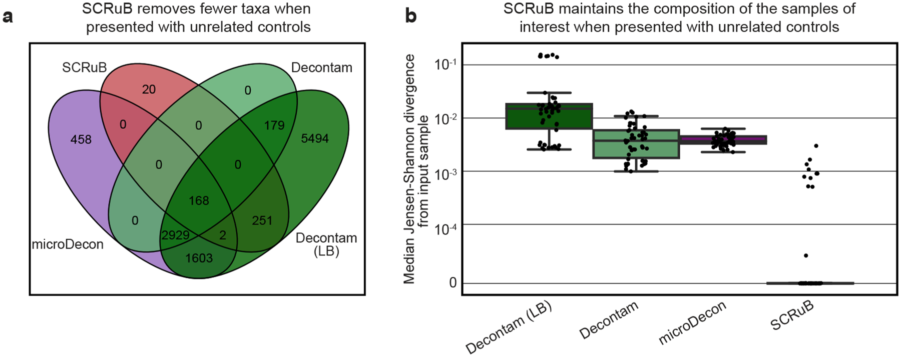
a, Venn diagram illustrating the taxa removed by each decontamination method, defined as a taxa with an aggregate sum greater than zero in the observed data, and an aggregate sum of zero in the decontaminated data. When presented with unrelated controls, SCRuB removed far fewer taxa than microDecon and either version of decontam, and the majority of taxa removed by SCRuB were also removed by microDecon and decontam (LB). b, Box and swarm plots (line, median; box, IQR; whiskers, 1.5*IQR) showing the median Jensen-Shannon divergence per simulation between simulated samples before and after decontamination with an unrelated control (Methods), across 50 simulated datasets of 88 samples and 8 negative controls. SCRuB is robust to non-informative controls, producing taxonomic compositions that are very close to the original, and significantly closer than alternative methods (one-sided Wilcoxon signed-rank p=4×10⁻¹⁰, p=8.8×10⁻¹⁰ and p=3.8×10⁻¹⁰ between SCRuB and microDecon, decontam or decontam (LB), respectively).

Extended Data Figure 7 |. SCRuB correctly accounts for well-to-well leakage.

a, Similar to Fig. 2f, showing the Jensen-Shannon divergence (y-axis) between the ground truth taxonomic composition, as defined by the experimental design of Minich et al.³¹ (Methods), and the taxonomic composition of the unprocessed dataset (“No decontamination”), or the dataset following decontamination by various methods (x-axis), and displayed separately for the 31 distinct low-prevalence (left) and 90 high-prevalence (right) monocultures. For low prevalence samples, SCRuB produced estimates that were significantly more similar to the ground truth compared to microDecon, decontam, decontam (LB), and to a restrictive approach (one-sided Wilcoxon p<10⁻⁴ in all cases). For the high prevalence samples, SCRuB performed comparably to decontam and microDecon (p=0.93, p=0.12, respectively) and outperformed no decontamination, restrictive, and decontam (LB) (p=10⁻⁸, p=8.7×10⁻¹⁷ and p=1.3×10⁻⁴, respectively). b-f, A simulation of a more complicated well-to-well leakage experiment, in which each taxa was placed in two monocultures instead of one. To simulate such a scenario, we randomly chose pairs of taxa, and then reassigned all reads assigned to one taxa across the experiment to the other, “focal”, taxa. For example, Minich et al. placed E. coli in well C10 (c), resulting in well-to-well leakage (d). We randomly selected well C3, containing a Corynbacterium species, and reassigned all Corynbacterium reads to E. coli (e). We then ran SCRuB on this simulated data, and evaluated the relative abundance of E. coli in its original well (b, f). We performed this 100 times, and examined the relative abundance of the focal taxa in its original well (b). In all cases, SCRuB accurately handled well-to-well leakage in this more complex scenario and avoided removing the taxa belonging to the focal monoculture.

Extended Data Figure 8 |. SCRuB correctly infers well-to-well leakage into negative controls in a metagenomic study of infant and maternal microbiomes.

a, The plate design used by Lou et al.^33,39, which included a negative control placed in the corner of each extraction plate. Through a strain-level analysis, Lou et al. identified well-to-well leakage into certain negative controls. b, When running SCRuB on each plate, using the MAG abundances of each sample (Methods), we identified well-to-well leakage into the negative control in two of the four plates that included a negative control. c, SCRuB’s predictions of well-to-well leakage were consistent with an assessment based on the results of Lou et al.’s strain-level analysis (Methods).

Extended Data Figure 9 |. Well-to-well leakage is more prominent during DNA extraction.

a,b, Plate layout during DNA extraction (a) and library preparation (b) of experiment 2 (Fig. 3a). 10 controls were included in the DNA extraction stage (triangles), and additional 7 in the library preparation stage (hexagon); a pair of each was away from other samples (“far samples”, purple). c, Box and swarm plot (line, median; box, IQR; whiskers, 1.5*IQR) showing the Jensen-Shannon divergence (y-axis) between human-derived samples adjacent to DNA extraction and library preparation controls and the various controls of each processing stage, stratified by adjacent and near controls (purple in a,b), and calculated from “raw” taxonomic compositions, without any decontamination. Samples are more similar to near than far controls, demonstrating well-to-well leakage occurring during both DNA extraction and library preparation. Samples are also more similar to near extraction controls than to near library controls, suggesting that well-to-well leakage is more prominent during DNA extraction. P, two-sided Mann-Whitney U; N, number of pairwise distances between relevant samples.

Extended Data Figure 10 |. SCRuB improves prediction of melanoma and treatment response.

a-f, Receiver operating characteristic (ROC) curves evaluating the pairwise classification accuracy of gradient boosted decision trees on data from patients with lung cancer, prostate cancer, melanoma, and controls, using data from Poore et al.²⁰ Compared to alternative decontamination methods, SCRuB offers classification accuracy that is on-par or improved, and improved accuracy compared to the original analyses in all cases. See Supplementary Table 1 for p values comparing between methods. Shaded area, 95% confidence interval. g, A Venn diagram enumerating the number of taxa completely removed by each decontamination methods applied to the tumor microbiome data from Nejman et al.¹⁸ SCRuB removed fewer taxa than alternative methods.

Supplementary Material

Supplementary Tables

Supplementary Table 1 | Exact P values displayed in figures.

Supplementary Table 2 | Experimental metadata and plate layouts of experiments performed. Refers to experiments described in Fig. 3.

Supplementary Table 3 | V1–V2 reads in control samples. The number of reads from the V1–V2 regions found in each of the samples from the experiments with human-derived samples (Fig. 3a; Methods). Samples with NA had no reads following DADA2 processing.

Data availability

Sequencing data from our experiments, along with all relevant metadata, was uploaded to SRA, accession PRJNA905430 (ref. 55). All other datasets analyzed in this study are publicly available. The college dormitory dataset²⁵ used in Fig. 1 and Extended Data Fig. 3–5 is available from the European Nucleotide Archive (ENA), accession ERP115809, and Qiita⁴¹, study ID 12470. The marine sediments dataset, used in Extended Data Fig. 3a,b, is available from Qiita⁴¹, study ID 11922. The fish microbiome dataset⁴², used in Extended Data Fig. 3c,d, is available from ENA, accession PRJEB54736, and Qiita⁴¹, study ID 13414. The Earth Microbiome Project soil dataset⁴³, used in Extended Data Fig. 3e,f, is available from ENA, accession PRJEB42019, and Qiita⁴¹, study ID 13114. The office dataset⁴⁴, used in Extended Data Fig. 3g,h, is available from ENA, accession PRJEB13115, and Qiita⁴¹, study ID 10423. The Central Park soil dataset⁴⁵, used in Extended Data Fig. 3i,j, is available from ENA, accession PRJEB6614, and Qiita⁴¹, study ID 2104. The gut metagenomic dataset⁴⁶, used in Extended Data Fig. 3k,l, is available from ENA, accession PRJEB50408, and Qiita⁴¹, study ID 13692. The negative controls dataset, used in Fig. 1, and Extended Data Fig. 3a–f,4,5 is available from Qiita⁴¹, study ID 12019; the one used in Extended Data Fig. 3g,h,k,l is available from ENA, accession PRJEB40903, and Qiita⁴¹, study ID 12201; and the one used in Extended Data Fig. 3i,j is available from ENA, accession PRJEB25617, and Qiita⁴¹, study ID 10333. The well-to-well leakage dataset³², is available from ENA, accession ERP115213. The plasma cfDNA data²⁰ is available from ENA, accessions ERP119598, ERP119596, and ERP119597; and Qiita⁴¹, study IDs 12667, 12691, and 12692. The tumor microbiome dataset¹⁸ is available from SRA, accession PRJNA624822. The processed data was obtained from Table S2 in ref. 18.

References

- 1.Salter SJ et al. Reagent and laboratory contamination can critically impact sequence-based microbiome analyses. BMC Biol. 12, 87 (2014). [DOI] [PMC free article] [PubMed] [Google Scholar]
- 2.Weyrich LS et al. Laboratory contamination over time during low-biomass sample analysis. Mol. Ecol. Resour 19, 982–996 (2019). [DOI] [PMC free article] [PubMed] [Google Scholar]
- 3.Kim D et al. Optimizing methods and dodging pitfalls in microbiome research. Microbiome 5, 52 (2017). [DOI] [PMC free article] [PubMed] [Google Scholar]
- 4.Eisenhofer R et al. Contamination in Low Microbial Biomass Microbiome Studies: Issues and Recommendations. Trends Microbiol. 27, 105–117 (2019). [DOI] [PubMed] [Google Scholar]
- 5.Weiss S et al. Tracking down the sources of experimental contamination in microbiome studies. Genome Biol. 15, 564 (2014). [DOI] [PMC free article] [PubMed] [Google Scholar]
- 6.Aagaard K et al. The placenta harbors a unique microbiome. Sci. Transl. Med 6, 237ra65 (2014). [DOI] [PMC free article] [PubMed] [Google Scholar]
- 7.Parnell LA et al. Microbial communities in placentas from term normal pregnancy exhibit spatially variable profiles. Sci. Rep 7, 11200 (2017). [DOI] [PMC free article] [PubMed] [Google Scholar]
- 8.Seferovic MD et al. Visualization of microbes by 16S in situ hybridization in term and preterm placentas without intraamniotic infection. Am. J. Obstet. Gynecol 221, 146.e1–146.e23 (2019). [DOI] [PMC free article] [PubMed] [Google Scholar]
- 9.de Goffau MC et al. Human placenta has no microbiome but can contain potential pathogens. Nature 572, 329–334 (2019). [DOI] [PMC free article] [PubMed] [Google Scholar]
- 10.Leiby JS et al. Lack of detection of a human placenta microbiome in samples from preterm and term deliveries. Microbiome 6, 196 (2018). [DOI] [PMC free article] [PubMed] [Google Scholar]
- 11.Kuperman AA et al. Deep microbial analysis of multiple placentas shows no evidence for a placental microbiome. BJOG: An International Journal of Obstetrics & Gynaecology 127, 159–169 (2020). [DOI] [PubMed] [Google Scholar]
- 12.Sinha R, Abnet CC, White O, Knight R & Huttenhower C The microbiome quality control project: baseline study design and future directions. Genome Biol. 16, 276 (2015). [DOI] [PMC free article] [PubMed] [Google Scholar]
- 13.Edmonds K & Williams L The Role of the Negative Control in Microbiome Analyses. The FASEB Journal 31, 940.3–940.3 (2017). [Google Scholar]
- 14.Schierwagen R et al. Trust is good, control is better: technical considerations in blood microbiome analysis. Gut 69, 1362–1363 (2020). [DOI] [PMC free article] [PubMed] [Google Scholar]
- 15.de Goffau MC et al. Recognizing the reagent microbiome. Nat Microbiol 3, 851–853 (2018). [DOI] [PubMed] [Google Scholar]
- 16.van der Horst J et al. Sterile paper points as a bacterial DNA-contamination source in microbiome profiles of clinical samples. J. Dent 41, 1297–1301 (2013). [DOI] [PubMed] [Google Scholar]
- 17.Olomu IN et al. Elimination of “kitome” and “splashome” contamination results in lack of detection of a unique placental microbiome. BMC Microbiol. 20, 1–19 (2020). [DOI] [PMC free article] [PubMed] [Google Scholar]
- 18.Nejman D et al. The human tumor microbiome is composed of tumor type-specific intracellular bacteria. Science 368, 973–980 (2020). [DOI] [PMC free article] [PubMed] [Google Scholar]
- 19.Pinto-Ribeiro I et al. Evaluation of the Use of Formalin-Fixed and Paraffin-Embedded Archive Gastric Tissues for Microbiota Characterization Using Next-Generation Sequencing. Int. J. Mol. Sci 21, 1096 (2020). [DOI] [PMC free article] [PubMed] [Google Scholar]
- 20.Poore GD et al. Microbiome analyses of blood and tissues suggest cancer diagnostic approach. Nature 579, 567–574 (2020). [DOI] [PMC free article] [PubMed] [Google Scholar] [Retracted]
- 21.Wang J et al. Translocation of vaginal microbiota is involved in impairment and protection of uterine health. Nat. Commun 12, 4191 (2021). [DOI] [PMC free article] [PubMed] [Google Scholar]
- 22.Lam SY et al. Technical challenges regarding the use of formalin-fixed paraffin embedded (FFPE) tissue specimens for the detection of bacterial alterations in colorectal cancer. BMC Microbiology 21, 297 (2021). [DOI] [PMC free article] [PubMed] [Google Scholar]
- 23.Allali I et al. Gut microbiome compositional and functional differences between tumor and non-tumor adjacent tissues from cohorts from the US and Spain. Gut Microbes 6, 161–172 (2015). [DOI] [PMC free article] [PubMed] [Google Scholar]
- 24.Marotz C et al. SARS-CoV-2 detection status associates with bacterial community composition in patients and the hospital environment. Microbiome 9, 132 (2021). [DOI] [PMC free article] [PubMed] [Google Scholar]
- 25.Richardson M, Gottel N, Gilbert JA & Lax S Microbial Similarity between Students in a Common Dormitory Environment Reveals the Forensic Potential of Individual Microbial Signatures. MBio 10, e01054–19 (2019). [DOI] [PMC free article] [PubMed] [Google Scholar]
- 26.Chen Q-L et al. Rare microbial taxa as the major drivers of ecosystem multifunctionality in long-term fertilized soils. Soil Biol. Biochem 141, 107686 (2020). [Google Scholar]
- 27.Smirnova E, Huzurbazar S & Jafari F PERFect: PERmutation Filtering test for microbiome data. Biostatistics 20, 615–631 (2019). [DOI] [PMC free article] [PubMed] [Google Scholar]
- 28.Davis NM, Proctor DM, Holmes SP, Relman DA & Callahan BJ Simple statistical identification and removal of contaminant sequences in marker-gene and metagenomics data. Microbiome 6, 226 (2018). [DOI] [PMC free article] [PubMed] [Google Scholar]
- 29.McKnight DT et al. microDecon: A highly accurate read‐subtraction tool for the post‐sequencing removal of contamination in metabarcoding studies. Environmental DNA 1, 14–25 (2019). [Google Scholar]
- 30.Shenhav L et al. FEAST: fast expectation-maximization for microbial source tracking. Nat. Methods 16, 627–632 (2019). [DOI] [PMC free article] [PubMed] [Google Scholar]
- 31.Knights D et al. Bayesian community-wide culture-independent microbial source tracking. Nat. Methods 8, 761–763 (2011). [DOI] [PMC free article] [PubMed] [Google Scholar]
- 32.Minich JJ et al. Quantifying and Understanding Well-to-Well Contamination in Microbiome Research. mSystems 4, e00186–19 (2019). [DOI] [PMC free article] [PubMed] [Google Scholar]
- 33.Lou YC et al. Using strain-resolved analysis to identify contamination in metagenomics data. bioRxiv 2022.01.16.476537 (2022) doi: 10.1101/2022.01.16.476537. [DOI] [PMC free article] [PubMed] [Google Scholar]
- 34.An U et al. STENSL: Microbial Source Tracking with ENvironment SeLection. mSystems 7, e0099521 (2022). [DOI] [PMC free article] [PubMed] [Google Scholar]
- 35.Bolyen E et al. Reproducible, interactive, scalable and extensible microbiome data science using QIIME 2. Nat. Biotechnol 37, 852–857 (2019). [DOI] [PMC free article] [PubMed] [Google Scholar]
- 36.Karstens L et al. Controlling for Contaminants in Low-Biomass 16S rRNA Gene Sequencing Experiments. mSystems 4, e00290–19 (2019). [DOI] [PMC free article] [PubMed] [Google Scholar]
- 37.Flores R et al. Collection media and delayed freezing effects on microbial composition of human stool. Microbiome 3, 33 (2015). [DOI] [PMC free article] [PubMed] [Google Scholar]
- 38.Adams RI, Bateman AC, Bik HM & Meadow JF Microbiota of the indoor environment: a meta-analysis. Microbiome 3, 49 (2015). [DOI] [PMC free article] [PubMed] [Google Scholar]
- 39.Lou YC et al. Infant gut strain persistence is associated with maternal origin, phylogeny, and traits including surface adhesion and iron acquisition. Cell Rep Med 2, 100393 (2021). [DOI] [PMC free article] [PubMed] [Google Scholar]
- 40.Hornung BVH, Zwittink RD & Kuijper EJ Issues and current standards of controls in microbiome research. FEMS Microbiol. Ecol 95, (2019). [DOI] [PMC free article] [PubMed] [Google Scholar]
Methods-only references
- 41.Gonzalez A et al. Qiita: rapid, web-enabled microbiome meta-analysis. Nat. Methods 15, 796–798 (2018). [DOI] [PMC free article] [PubMed] [Google Scholar]
- 42.Minich JJ et al. Host biology, ecology and the environment influence microbial biomass and diversity in 101 marine fish species. Nat. Commun 13, 6978 (2022). [DOI] [PMC free article] [PubMed] [Google Scholar]
- 43.Shaffer JP et al. Standardized multi-omics of Earth’s microbiomes reveals microbial and metabolite diversity. Nat Microbiol 7, 2128–2150 (2022). [DOI] [PMC free article] [PubMed] [Google Scholar]
- 44.Chase J et al. Geography and Location Are the Primary Drivers of Office Microbiome Composition. mSystems 1, e00022–16 (2016). [DOI] [PMC free article] [PubMed] [Google Scholar]
- 45.Ramirez KS et al. Biogeographic patterns in below-ground diversity in New York City’s Central Park are similar to those observed globally. Proc. Biol. Sci 281, 20141988 (2014). [DOI] [PMC free article] [PubMed] [Google Scholar]
- 46.Hanes D et al. The gastrointestinal and microbiome impact of a resistant starch blend from potato, banana, and apple fibers: A randomized clinical trial using smart caps. Front Nutr 9, 987216 (2022). [DOI] [PMC free article] [PubMed] [Google Scholar]
- 47.Shaffer JP et al. A comparison of DNA/RNA extraction protocols for high-throughput sequencing of microbial communities. Biotechniques 70, 149–159 (2021). [DOI] [PMC free article] [PubMed] [Google Scholar]
- 48.Ruiz-Calderon JF et al. Walls talk: Microbial biogeography of homes spanning urbanization. Sci Adv 2, e1501061 (2016). [DOI] [PMC free article] [PubMed] [Google Scholar]
- 49.Robin X et al. pROC: an open-source package for R and S to analyze and compare ROC curves. BMC Bioinformatics 12, 77 (2011). [DOI] [PMC free article] [PubMed] [Google Scholar]
- 50.Callahan BJ et al. DADA2: High-resolution sample inference from Illumina amplicon data. Nat. Methods 13, 581–583 (2016). [DOI] [PMC free article] [PubMed] [Google Scholar]
- 51.Annavajhala MK et al. Oral and gut microbial diversity and immune regulation in patients with HIV on antiretroviral therapy. mSphere 5, e00798–19 (2020). [DOI] [PMC free article] [PubMed] [Google Scholar]
- 52.Graspeuntner S, Loeper N, Künzel S, Baines JF & Rupp J Selection of validated hypervariable regions is crucial in 16S-based microbiota studies of the female genital tract. Sci. Rep 8, 9678 (2018). [DOI] [PMC free article] [PubMed] [Google Scholar]
- 53.Herlemann DP et al. Transitions in bacterial communities along the 2000 km salinity gradient of the Baltic Sea. ISME J. 5, 1571–1579 (2011). [DOI] [PMC free article] [PubMed] [Google Scholar]
- 54.Law CW, Chen Y, Shi W & Smyth GK voom: Precision weights unlock linear model analysis tools for RNA-seq read counts. Genome Biol. 15, R29 (2014). [DOI] [PMC free article] [PubMed] [Google Scholar]
- 55.Austin GI et al. Contamination benchmark using human-derived samples. BioProject PRJNA905430. NCBI Sequence Read Archive. https://www.ncbi.nlm.nih.gov/bioproject/PRJNA905430 (2023).
- 56.Austin GI, Shenhav L & Korem T SCRuB. GitHuB https://github.com/Shenhav-and-Korem-labs/SCRuB (2023).
- 57.Friedman J, Hastie T & Tibshirani R Regularization paths for generalized linear models via coordinate descent. J. Stat. Softw 33, 1–22 (2010). [PMC free article] [PubMed] [Google Scholar]
- 58.Shenhav L, Korem T, Austin G. Contamination source modeling with SCRuB improves cancer phenotype prediction from microbiome data [Source Code]. 10.24433/CO.2307706.v1 (2023). [DOI] [PMC free article] [PubMed]
- 59.Wickham H et al. Welcome to the tidyverse. J. Open Source Softw 4, 1686 (2019). [Google Scholar]
- 60.Chen T & Guestrin C XGBoost. in Proceedings of the 22nd ACM SIGKDD International Conference on Knowledge Discovery and Data Mining (ACM, 2016). doi:10.1145/2939672.2939785. [Google Scholar]
Associated Data
This section collects any data citations, data availability statements, or supplementary materials included in this article.
Supplementary Materials