Learning Brain Dynamics of Evolving Manifold Functional MRI Data Using Geometric-Attention Neural Network

Abstract

Functional connectivities (FC) of brain network manifest remarkable geometric patterns, which is the gateway to understanding brain dynamics. In this work, we present a novel geometric-attention neural network to characterize the time-evolving brain state change from the functional neuroimages by tracking the trajectory of functional dynamics on high-dimension Riemannian manifold of symmetric positive definite (SPD) matrices. Specifically, we put the spotlight on learning the common state-specific manifold signatures that represent the underlying cognition. In this context, the driving force of our neural network is tied up with the learning of the evolution functionals on the Riemannian manifold of SPD matrix that underlies the known evolving brain states. To do so, we train a convolution neural network (CNN) on the Riemannian manifold of SPD matrices to seek for the putative low-dimension feature representations, followed by an end-to-end recurrent neural network (RNN) to yield the time-varying mapping function of SPD matrices which fits the evolutionary trajectories of the underlying states. Furthermore, we devise a geometric attention mechanism in CNN, allowing us to discover the latent geometric patterns in SPD matrices that are associated with the underlying states. Notably, our work has the potential to understand how brain function emerges behavior by investigating the geometrical patterns from functional brain networks, which is essentially a correlation matrix of neuronal activity signals. Our proposed manifold-based neural network achieves promising results in predicting brain state changes on both simulated data and task functional neuroimaging data from Human Connectome Project, which implies great applicability in neuroscience studies.

I. Introduction

DEEP learning has achieved striking successes in many areas, such as computer vision and medical imaging [1], [2]. Since humans understand the natural objects in the real world using 3D cartesian coordinates, it is straightforward to use regular data structures such as arrays and grid matrices to model images and video footage. In contrast, learning from instances with an irregular data structure such as graph and tensor-like data is much more challenging, which often requires tailored manifold algebra to capture the latent geometric patterns.

Due to many well-studied mathematical properties on the Riemannian manifold of SPD matrix, tremendous efforts have been made to learn from the manifold instances of SPD matrices. For example, the handcrafted manifold-based descriptor is proposed in [3] to classify the hand gesture using the covariance matrix of landmarks. In the medical imaging area, the SPD-based regression model has been applied to characterize the tractography of white matter fibers in DTI (diffusion tensor imaging) data, where the Lie algebra is used to operate SPD matrices in the log-Euclidian framework. Following the deep learning cliché of convolution and pooling, a Riemannian network for SPD matrix learning is proposed in [4] by replacing the convolutional and ReLU layers in CNN with the BiMap and ReEig layers that use log-Euclidean operations. Recently, a kernel convolution approach on the SPD matrix has been used in the neural network for skeleton-based hand gestures and actions [5], [6], where the convolutional kernels are essentially SPD matrices [7].

Despite the importance of learning manifold feature representations from the SPD matrices, the characterization of dynamics from the evolving function of SPD matrices is in high demand in predicting time events and uncovering evolutionary patterns. For instance, the in-vivo functional MRI (Magnetic Resonance Imaging) technology allows us to study the connection of distant brain regions by measuring the covariance of functional fluctuations through BOLD (Blood-Oxygen-Level-Dependence) signals, which lands in a functional brain network in the form of SPD correlation matrix [8]. Since mounting evidence shows the cognitive status changes even in the resting state, the sliding window technique is used to capture functional dynamics using a set of functional brain networks [9]. Therefore, the understanding the how brain function supports cognition is highly dispensable on the characterization of the dynamic behavior of evolving SPD matrix trajectories.

However, little attention has been paid to learning the evolutionary function from a discrete set of SPD matrices. To address this challenge, we propose a novel manifold-based neural network to jointly learn the low-dimensional manifold feature representations and predict the trajectory of SPD matrices on the Riemannian manifold. Our major contributions include:

• We regard the input manifold instances as the manifold functional data where the latent temporal relationships are characterized by a continuous function on the Riemannian manifold of SPD matrices.

• To cast the learning problem into a supervised scene, we assume each SPD matrix is associated with a state. In this regard, we boil down the search for the evolutional manifold function of SPD matrices into the temporal stratification problem of SPD matrices on the Riemannian manifold that is required to be aligned with the known state changes.

• We integrate a geometric-attention mechanism in learning the low-dimensional manifold feature representation, which allows us to understand the local geometric patterns associated with the underlying state.

In method exploration, we apply our proposed manifold-based neural network to characterize the dynamic behavior in connectivity without requiring prior knowledge of brain states (as shown in Figure 1). The input consists of a sequence of functional connectivity (FC) matrices, where each FC matrix is an SPD instance describing the functional network in a certain sliding window. The output is a time-varying manifold function of the SPD matrix that predicts the change of brain states. Extensive experiments have been conducted to evaluate the learning performance on both simulated data and real task fMRI data, where our proposed geometric-attention neural network achieves promising prediction results in terms of accuracy and replicability.

Fig. 1.

The overview of our work. The overarching goal of our method is to learn the brain dynamic behavior in the time series of SPD matrices. Left: each time-evolving brain scan lies on the manifold characterized by the black point. Right: the inferred temporal relationships are assigned in different colors and attraction basins of modes on the manifold.

II. Related Works

We provide a quick review for recent works on deep neural networks on SPD manifold and current state-of-the-art methods of brain state change detection.

A. Deep Neural Network on SPD Manifold

Many manifold-based deep neural networks have been proposed in various computer vision applications such as object classification [10], recognition [11], and tracking [12]. Current state-of-the-art methods share the common principle of learning, that is, reducing the dimension of the input high-dimensional SPD matrix while maintaining the intrinsic geometric of symmetric and positive definite. In general, the current neural network on the Riemannian manifold of the SPD matrix consists of two disjoint learning components. Riemannian manifold algebra is used in the dimension reduction layers, such as the log-Euclidean in [4] and SPD kernel convolution in [7]. After that, the learned manifold feature representation (lies on the Riemannian manifold) is often stretched into a vector in the Euclidean space for the conventional fully connected neural network. By doing so, it is relatively easier to backpropagate the training error and train the neural network. However, the network neuroscience insight of the learned features might be less explainable due to the undermining of data geometry after the fully connected neural network.

B. Brain State Change Detection

In the past decades, various statistical inference and machine learning approaches have been proposed to detect brain state changes from fMRI data. For example, a Bayesian model has been used to characterize the probabilistic relationship between the observed BOLD signal and the cognition state [9]. Although statistical inference holds potential power to track functional dynamics, the intensive computational cost limits its application only to small-scale networks [13]. Unsupervised clustering, such as k-means and locally linear embedding (LLE) is another commonly used technique to detect the change by considering each FC matrix constructed within the sliding window as the feature vector [14]. Recently, a graph-based learning change detection method is emerging, which aims at learning the dynamic graph embedding via integrating the Fourier bases and Eigen bases spanned by the subspace of individual fMRI data [13]. Note, most methods vectorize the entire FC matrix into a data array and form the FC-based features for change detection. Thus, the whole scanning period can be partitioned into several segments, where the FC-based feature vectors are supposed to be not only homogenous in each segment but also associated with a specific cognitive task. Since the trajectory of functional connectivities is continuous in the temporal domain, recurrent neural network (RNN) technique has been used to identify the change of brain states based on the functional profiles in [15], where the coefficients after FC matrix decomposition are considered as the input to RNN.

As Pearson’s correlation is often used to characterize functional connectivity between two distinct brain regions, each functional brain network is essentially an instance of SPD matrix lying on the Riemannian manifold. In the following, we present our manifold-based neural network to learn the time-varying functional from the input SPD matrices, where each SPD matric is regarded as a landmark on the trajectory on the Riemannian manifold. To our knowledge, our work is the first deep learning approach that captures the dynamics of SPD instances on the Riemannian manifold.

III. Method

In this section, we first interpret the preliminaries concerning SPD matrices in Section III-A. Section III-B and Section III-C elaborately introduce the proposed method in a general manner. We eventually explore our method to brain change detection in Section III-D.

A. Preliminaries on Riemannian Geometry of SPD Matrices

A real $n\times n$ SPD matrix $X\in {Sym}_n^{+}$ satisfies the property that for any non-zero vector $\alpha \in {\mathbb{R}}^n,{\alpha }^{T}X\alpha >0$. We denote ${𝒯}_Xℳ$ as the tangent space of the Riemannian manifold $ℳ$ at $X$. Herein, we use the popular Log-Euclidean algebra [16] to project any SPD matrix $X$ on the manifold to its tangent space by the logarithm map $P=\log \left(X\right)={\mathrm{\Phi }}^T\log \left(\mathrm{\Lambda }\right)\mathrm{\Phi }(P\in \left.{𝒯}_Iℳ\right)$, where $\mathrm{\Lambda }\in {\mathbb{R}}^{n\times n}$ and $\mathrm{\Phi }\in {\mathbb{R}}^{n\times n}$ are the eigenvalue and eigenvector matrix after applying SVD (Singular Value Decomposition) on $X$, i.e., $X={\mathrm{\Phi }}^T\mathrm{\Lambda }\mathrm{\Phi }$. Based on Lie group algebra, $P$ is a symmetric matrix. Hence, there exists a unique SVD on $P={\mathrm{\Psi }}^T\mathrm{\Delta }\mathrm{\Psi }$, resulting in the Eigenvalue matrix $\mathrm{\Delta }$ and Eigenvector matrix $\mathrm{\Psi }$. Then, we use the exponential operation to map the tangent vector $P$ back to the manifold $ℳ$ by $\exp \left(P\right)={\mathrm{\Psi }}^T\exp \left(\mathrm{\Delta }\right)\mathrm{\Psi }$. Furthermore, the geodesic distance between two SPD matrices $X$ and $Y$ is given by $d(X,Y)=\parallel \log \left(X\right)-\log \left(Y\right){\parallel }_F$.

The following properties of SPD matrix allow us to maintain the data geometry in the feed-forward process of the deep neural network.

Proposition 1: Given two SPD matrices $A\in Sy{m}_n^{+}$ and $B\in {Sym}_n^{+}$, the summation $A+B$ is also an SPD matrix.

Proof: It is apparent that $A+B$ is symmetric. $\forall \alpha \in {\mathbb{R}}^n,{\alpha }^T(A+B)\alpha =a^{T}A\alpha +{\alpha }^{T}B\alpha >0$ since $A$ and $B$ are both SPD matrices.

Proposition 2: Given two SPD matrices $A\in Sy{m}_m^{+}$ and $B\in {Sym}_n^{+}$, the assembled matrix $C=diag(A,B)=\left[\begin{array}{cc}A& 0_{m\times n}\\ 0_{n\times m}& B\end{array}\right]$ is a SPD matrix, i.e., $C\in {Sym}_{(m+n)}^{+}$.

Proof: First, $C$ is symmetric. Given the vectors $\alpha \in {\mathbb{R}}^m$ and $\beta \in {\mathbb{R}}^n$, the concatenated vector $\mu ={\left[\begin{array}{ll}\alpha & \beta \end{array}\right]}^T\in {\mathbb{R}}^{m+n}$. Since A and B are both symmetric and positive definite, ${\mu }^{T}C\mu =\left(a^{T}A\alpha +{\beta }^{T}B\beta \right)>0$, which proves $C$ is a SPD matrix.

Based on the Proposition 2, it is straightforward to derive:

Proposition 3: Given a SPD matrix $A\in Sy{m}_n^{+}$, the zero padding $\left[\begin{array}{ll}\theta & 0\\ 0& A\end{array}\right]$ is a SPD matrix too, where $\theta$ is a small positive value.

In the following, we propose a geometric attention neural network to learn the dynamics of evolving manifold data from a discrete set of SPD matrices, as shown in Figure 1. First, in Section III-B, we exploit an SPD-based CNN (SPD-CNN) to learn the feature representation on the Riemannian manifold. Also, a geometric attention mechanism (GAM) is proposed to discover the significant latent geometric patterns in SPD matrices. In Section III-C, a manifold-based mean shift process is devised to characterize and fit the evolutionary trajectories of SPD matrices in the manner of RNN (short for MMS-RNN). In Section III-D, we apply our method for detecting dynamic functional brain cognitive state change with a task-specific loss function.

B. Manifold Feature Representation Learning

Enlighted by the recent work in [7], we seek for the putative SPD feature representations by reducing the dimensionality of SPD matrix while preserving the data geometry on the Riemannian manifold. Similar to the widely-used CNN architecture, the building block of our SPD-CNN consists of a convolution layer and a non-linear activation layer, as shown in Figure 2.

Fig. 2.

A convolution neural network (CNN) on the Riemannian manifold of SPD matrices.

1). Convolution on Individual SPD Matrix:

Suppose the convolution kernel $W\in {Sym}_k^{+}$ is a $k\times k$ SPD matrix. It has been proven in [6] that the convolution of input $n\times n(n>k)$ SPD matrix $X\in {Sym}_n^{+}$ using $W$ yields a $(n-k+1)\times (n-k+1)$ SPD matrix $Y\in Sy{m}_{n-k+1}^{+}$, where each element $y_{ij}(i,j=1,\dots ,n-k+1)$ in $Y$ is the summation of element-to-element production between $W$ and the corresponding matrix block centered at $(i,j)$ in $X$. Since it is challenging to optimize each element in $W$ while maintaining it as a SPD matrix, the LU-like factorization is applied to approximate the learning of SPD kernel matrix $W$ on the Riemannian manifold to the regular $k\times k$ matrix $V\in {\mathbb{R}}^{k\times k}$ in the vector space by $W=V^{T}V+\epsilon I_{k\times k}$, where $\epsilon$ is a scalar to enforce the positive definite of $W$. Following the convention in CNN, we use $Y=X⊛W$ to denote the above convolution process on SPD matrix $X$ using SPD convolution kernel $W$.

2). Non-Linear Activation:

Similar to the ReLU layer in CNN, we introduce non-linearity by applying element-wise exponential to $Y$, which does not violate the symmetry and positive definite of $Y$. Note, we normalize the output of SPD matrix convolution by $Y=Y/\parallel Y{\parallel }_F$ before the activation operation, which prevents $Y$ from being degenerated. In the following, we use $ReLu(\cdot )$ to denote the function of non-linear activation.

3). Geometric Attention Mechanism:

The geometric attention map for each SPD matrix $X$ is coupled with the underlying SPD convolution kernel $W$, which can be formulated as $G(X,W)=\frac{ReLu(X⊛W)}{\max ⊛\left(ReLu\right(X⊛W)}$. Our attention map captures the geometric attention in the sense that it is associated with the SPD kernel $W$ which is part of the parameters in the entire neural network. As shown in Figure 3, we first pad zeros to the input SPD matrix $X$ since we prefer the attention map $G$ has the same size as the input $X$. Note, we fill in a very small positive value on the diagonal of $X$ to guarantee the SPD property (proved by Proposition 3). Since each element in $G$ ranges from 0 to 1 after dividing by the maximum response of convolution output, the Hadamard product $G\circ X$ is also a SPD matrix (proved by Schur product theorem¹), which allows to implement a simple yet efficient way to integrate the estimated attention maps into the manifold feature representation learning by replacing $X$ with $G\circ X$ as the input to the SPD convolution layer.

Fig. 3.

Illustration of geometric attention mechanism.

4). Overall Network Architecture of SPD-CNN:

Suppose the input is the SPD matrix $X$. We first learn the geometric attention map $G(X,W)$ and further calculate $G\circ X$ as the input of the next convolutional layer. Given $r^{\left(1\right)}$ SPD kernels ${\mathit{W}}^{\left(1\right)}=\left\{W_u^{\left(1\right)}\mid u=1,\dots ,r^{\left(1\right)}\right\}$, where we use the superscript to denote the index of the underlying convolutional layer $l(l=1,\dots ,L)$. Thus, the output of the $1^{\text{st}}$ convolutional layer consists of $r^{\left(1\right)}$ SPD matrices ${\mathit{Y}}^{\left(1\right)}=\left\{Y_u^{\left(1\right)}\mid u=1,\dots ,r^{\left(1\right)}\right\}$, which constitute the multi-channel input for the next layer. To that end, we train $r^{\left(1\right)}$ attention maps for each channel followed by $r^{\left(1\right)}$ convolutional layers. Similarly, we use $r^{\left(2\right)}$ SPD kernels in the $2^{\text{nd}}$ convolution layer and yield in total $r^{\left(2\right)}\times r^{\left(1\right)}$ output SPD matrices. To keep track of the learning complexity, we resort to entrywise sum of matrices over the $r^{\left(1\right)}$ channels and form the output ${\mathit{Y}}^{\left(2\right)}=\left\{Y_u^{\left(2\right)}\mid u=1,\dots ,r^{\left(2\right)}\right\}$. Inspired by the mean pooling used in the Grassmannian manifold-based network [17], we design a manifold-based average pooling on each channel to reduce the dimensionality of FC matrices. The pooling procedure consists of the following three steps: (1) mapping the FC matric ${\mathit{Y}}^{\left(2\right)}$ into the tangent space for performing Euclidean metric, (2) calculating the classic mean pooling used in the conventional neural network for reducing the matrix dimension, (3) transforming the low-dimensional matrix back into the manifold space by conducting the exponential operation (detailed in Section III-A) to preserve SPD property. Thus, the building block of our SPD-CNN is a combination of one geometric attention layer followed by the convolution layer, where the number of input channels in the next layer is equivalent to the number of the SPD kernels used in the current convolution layer.

By repeating these steps, we eventually obtain $r^{\left(L\right)}$ SPD matrices ${\mathit{Y}}^{\left(L\right)}=\left\{Y_u^{\left(L\right)}\mid u=1,\dots ,r^{\left(L\right)}\right\}$ for each input $X$, where each of them is expected to have a much smaller size after $L$ convolution layers. Based on Proposition 2, we can construct a new SPD matrix $Z$ by assembling each low-dimension $Y_u^{\left(L\right)}$ along the diagonal line, i.e., $Z=diag\left({\mathit{Y}}^{\left(L\right)}\right)$, which is considered as the manifold feature representation of $X$. It is worth noting that (1) the dimensionality of $Z$ is smaller than the original input $X$ since each $Y_u^{\left(L\right)}$ is in low dimension; (2) $Z$ is actually a fairly sparse matrix which forms a compact feature representation for learning the dynamics on the Riemannian manifold below.

C. Learning the Evolution of Manifold Function

Suppose we have a time series of the manifold feature representations $\mathit{Z}=\left\{Z\left(t\right)\mid t=1,\dots ,T,Z\left(t\right)\in Sy{m}^{+}\right\}$, where each SPD matrix $Z\left(t\right)$ is associated with a state variable $o\left(t\right)\in \mathbb{R}$. In this context, we are interested in predicting the evolution function of state change from the manifold time series $\left\{Z\right(t\left)\right\}$.

1). Stratifying Manifold Instances via Mean-Shift:

One of the efficient solutions is to cluster $\left\{Z\right(t\left)\right\}$ in the temporal domain via mean shift. Since each $Z\left(t\right)$ lies on the Riemannian manifold of the SPD matrix, we can stratify $\left\{Z\right(t\left)\right\}$ on the manifold by iteratively performing the following three steps:

1. Construct a Gaussian kernel $h\left(t,t^{\prime }\right)=\exp \left(-{\left[\frac{d\left(Z\left(t\right),Z\left(t^{\prime }\right)\right)}{\sigma }\right]}^2\right)$ where $d\left(Z\left(t\right),Z\left(t^{\prime }\right)\right)$ is the geodesic distance between $Z\left(t\right)$ and $Z\left(t^{\prime }\right)$, and $\sigma$ is the kernel width;

2. Compute the mean-shift vector $\xi \left(t\right)=\frac{{\sum }_{t=1}^{T}h\left(t,t^{\prime }\right)\left[\log \left(Z\left(t^{\prime }\right)\right)-\log \left(Z\right(t\left)\right)\right]}{{\sum }_{t=1}^{T}h\left(t,t^{\prime }\right)}$;

3. Update $Z\left(t\right)$ through mean shift by $Z\left(t\right)\leftarrow \exp \left(\log \right(Z\left(t\right)+\xi \left(t\right))$. Note, the $\log (\cdot )$ and $\exp (\cdot )$ used in Lie algebra are Riemannian inverses of Logarithm and Exponent maps (explained in Section III-A), respectively.

2). End-to-End Network of Mean Shift on Riemannian Manifold by RNN:

The conventional mean-shift algorithm operates in an unsupervised manner, where the mean-shift process can be described using a non-linear function $\mathscr{H}\left(\right\{Z\left(t\right)\},\sigma )$, where $\sigma$ is the hyper-parameter. Since the state label $o\left(t\right)$ is known for each $Z\left(t\right)$, we propose to implement the iterative mean-shift process via a RNN model as shown in Figure 4. Specifically, the input to mean-shift RNN (MS-RNN) is the output $\left(\left\{Z\right(t){\}}_{t=1}^T\right)$ of SPD-CNN. There are two recurrent learning components in our mean-shift RNN: one for calculating mean shift vector ${\xi }^{\left(ϵ\right)}\left(t\right)$ based on the mean-shift location $Z^{(ϵ-1)}\left(t\right)$ in the previous iteration ($ϵ$ is the index of iterations), and another one for shifting $Z^{(ϵ-1)}\left(t\right)$ to the new location $Z^{\left(ϵ\right)}\left(t\right)$ on the manifold. Since the output of mean-shift RNN is supposed to collapse at several on the manifold, the possible loss measuring the disparity between the known state $o\left(t\right)$ and the current temporal clustering result can be propagated back to the SPD-CNN to steer the manifold feature representation learning, which yields an end-to-end network solution in a supervised manner for brain state change detection described below.

Fig. 4.

The illustration of our manifold-based mean shift RNN. Top: two recurrent learning components in our MMS-RNN; Bottom: the mean shift process in each iteration on SPD manifold.

D. Method Exploration – Brain State Change Detection

In this section, we apply our method for detecting dynamic functional brain cognitive state change. The framework of our method applied to the brain network is shown in Figure 5. We first introduce the construction of SPD matrix (the input $X$ of our network) from the brain network, followed by the task-specific loss function.

Fig. 5.

The framework of our method for detecting dynamic behavior in the functional brain network.

1). Construction of FC Matrices:

Suppose a training data has $M$ fMRI scans, each scan is partitioned the brain network into $N$ regions and has been processed into $N$ mean time courses of BOLD signals (the middle of Figure 5). The BOLD signal has $T$ time points at each region. Thus, the data matrix can be formulated as $S={\left[s_t\right]}_{t=1}^T\in {\mathbb{R}}^{N\times T}$, which represents the whole brain BOLD signals, where each $s_t\in {\mathbb{R}}^N$ is a $N$-length column vector. Without loss of generality, we assume that there are in total $Q$ brain states $\mathrm{\Gamma }=\left\{{\gamma }_q\mid q=1,\dots ,Q\right\}$ during each scan (the left panel of Figure 5). After that, we adopt the sliding window scheme to capture the functional dynamics of the brain network, at each time point $t(1\le t\le T)$, the width of the sliding window is set to $\varpi (\varpi >0)$ and the centered at $t$. Thus, we construct FC matrix $X\left(t\right)={\left[x_{ij}^t\right]}_{i,j=1}^N$, where $x_{ij}^t$ denotes the Pearson’s correlation of truncated BOLD signals (within the sliding window centered at $t$) between $i^{th}$ and $j^{\text{th}}$ regions. To strictly ensure the positive definite property in each $X\left(t\right)$, we further add a small constant disturbance $\left({10}^{-4}\right)$ along the diagonal line of eigenvalues of $X\left(t\right)$ to ensure the SPD property of $X\left(t\right)$. By doing so, we can generate a series of FC matrices ${\mathit{X}}_m={\left\{X_m\left(t\right)\right\}}_{t=1}^T,(m=1,\dots ,M)$ for each fMRI scan (the middle of Figure 5).

2). State Change-Based Loss Function for the Learned FC Representations:

It is clear that the high-dimensional SPD matrices ${\mathit{X}}_m$ for $m^{\text{th}}$ subject is the input of our network. The learned low-dimensional FC putative representation through the proposed network is $Z_m={\left\{Z_m\left(t\right)\right\}}_{t=1}^T$ of $m^{th}$ subject. Since our goal is to stratify $Q$ cognitive tasks based on ${\mathit{Z}}_m$ for the new fMRI scan, we expect the putative FC representation $Z_m\left(t\right)$ has high similarity to other $Z_m\left(t\right)\left(t\ne t^{\prime }\right)$ if $t$ and $t^{\prime }$ are associated with the same cognitive task, i.e., $o_m\left(t\right)=o_m\left(t^{\prime }\right)$, in which label $o_m\left(t\right)$ and $o_m\left(t^{\prime }\right)$ that denote the pre-defined task labels (regarded as the prior knowledge, i.e., ground truth). Hence, the geodesic distance $d_m^{t{t}^{\prime }}={∥\log \left(Z_m\left(t\right)\right)-\log \left(Z_m\left(t^{\prime }\right)\right)∥}_F$ between the learned FC representations belonging to the same states on SPD manifold is required to be as small as possible. In light of this, the loss function $\ell$ for learning task-specific FC representation is given by:

$$\ell =\sum _{m=1}^M\sum _{t,t^{\prime }=1}^T\left({\mathbf{1}}_{\left\{o_m(t)=o_m\left(t^{\prime }\right)\right\}}{d}_m^{t{t}^{\prime }}-{\mathbf{1}}_{\left\{o_m(t)\ne o_m\left(t^{\prime }\right)\right\}}{\left[d_m^{t{t}^{\prime }}-\alpha \right]}_{+}\right)$$ (1)

where $\alpha$ is a flexible scalar that controls the maximum margin for different states/tasks. We employ the stochastic gradient descent (SGD) method to optimize network parameters.

IV. Experiments

A. Implemental Details

Our network is composed of GAM, SPD-CNN and MMS-RNN, as shown in Figure 5. The size of convolution kernel $k$ is set to 5, the scalar $\alpha$ is set as $0,\epsilon$ is set to ${10}^{-4}$, the kernel width $\sigma$ is initialized to 0.1, the SGD parameters with learning rate set to 0.005, weight decay is ${10}^{-5}$, momentum is 0.9.

We evaluate our geometric attention neural network on the functional neuroimages from Human Connectome Project (HCP) [18]. We compare the performance of detecting brain state change with the following seven counterpart methods:

1. Classic spectral clustering method (SC) and k-means clustering method (K-means) based on the vectorized brain network data;

2. A recent clustering method by seeking for density peaks (DP) of the data distribution [19] which also casts brain network as a vector.

3. A graph-based change detection method (dGE) [20] that first projects the brain network into a graph spectrum domain and then applies the temporal clustering on the graph spectrum coefficients;

4. A recently published spectral clustering with graph-based neural network (SCGNN) method [21]. Note, SCGNN is designed for solving the graph cut problem in image segmentation. We adapt this deep learning work into clustering temporal graphs.

5. A manifold-based deep neural network for SPD matrices analysis method (SPDNet) [4]. We use the learned low dimensional features as the input to the conventional spectral clustering method.

6. A manifold-based neural work for brain change point detection (CPDNet) [22]. CPD-Net is our previous work which has a similar design. Compared to our proposed method, we use the convolutional approach to extract features with attention mechanisms, and our method is an end-to-end solution.

Since we apply the above methods to predict the state changes based on the observed time series of SPD matrices, the detection accuracy is measured by purity score [13], which intuitively reveals the matching degree between ground truth and the predictive clustering results. It has been widely used in machine learning for appraising clustering accuracy.

B. Evaluation on Simulated Data

1). Simulated Data Generation:

First, we use SimTB toolbox [23] to generate the simulated fMRI time series with three brain states $(Q=3)$. As shown in Figure 6 (a), the three brain states are simulated where each underlying FC matrix consists of three modules (communities) along the diagonal line (state 1 in blue, state 2 in green, and state 3 in orange). For each possible pair of nodes with the same module, the degree of connectivity is set to one. No connection is allowed across modules [20, 24]. We generate 2000 samples (including 1000 testing samples), where each sample has 300 time points and each brain state lasts 100 seconds.

Fig. 6.

(a): The example of simulated data with three brain states. (b): The detection accuracy of brain state changes (vertical axis) with respect to window sizes, noise levels, and network dimensions (horizontal axis). (c): The results of our geometric attention mechanism.

2). Sensitivity Analysis on Different Window Size:

We evaluate the effect of the window size ($\varpi =10-60$ time points) on the detection accuracy of FC changes. Figure 6 (b, left panel) demonstrates the detection results by our method (in pink), SC (in blue), DP (in green) dGE (in brown), SPDNet (in cyan), CPDNet (in gray), SCGNN (in purple) and K-means (in orange) where our network yields the highest accuracy in all settings of the window sizes. Based on the results, we opt for $\varpi =60$ to perform the following simulated analyses.

3). Robustness Analysis to Noise:

We evaluate the performance of the proposed method affected by different-level noises. To this end, we add uncorrelated additive Gaussian noise to the generated BOLD signals with different-level signal-noise ratios (SNR). The noise levels range from $60dB$ to $0.5dB$. Figure 6 (b, middle panel) demonstrates the change detection results regarding different-level noises. It is clear that our geometric-attention neural network is much more robust to the noises.

4). Scalability Regarding Network Size:

To further verify the stability of our method, we change the brain parcellation number from $10\times 10$ to $100\times 100$. Figure 6 (b, right panel) illustrates the change detection results, which reflect our method consistently outperforms the other seven methods.

5). Visualization on the Identified Network Attention:

Figure 6 (c) shows the result of geometric attention module, it is clear that we can observe that the learned geometric attention patterns are closely aligned with the change of network topology.

C. Application on Task-Based fMRI Data

1). Data Description:

In this experiment, we select 743 healthy subjects (splitting 378 training set, 47 validation set and 318 testing set) involved working memory task-based fMRI data from the HCP database [18]. Each subject has the test and retest fMRI scans. The working memory tasks in each fMRI scan contain 2-back and 0-back task events of body, place, face, and tools, as well as fixation periods. We utilized the HCP minimally processed data that included distortion correction and had been warped to standard space [25]. Each fMRI scan consisted of 393 scanning time points. We used two scans for each subject, the left-to-right (LR) and right-to-left (RL), with one being used for test and the other for retest analyses. Given the sensitivity of dynamic networks to head motion and global signal, we chose to use the state-of-the-art correction technique ICA-AROMA [26], [27] to address this concern. For each scan, AROMA was used to remove high-frequency, edge, and motion signal artifacts that are commonly associated with head motion. A band-pass filter $(0.009-0.08\mathrm{Hz})$ was then applied to each scan and a regression was performed using mean tissue signals to remove any remaining global signal artifacts (GM, WM, and CSF). In addition, the six movement parameters and derivatives were included in the regression to address any further signal that was correlated with motion. The brain was parcellated into 268 brain regions using the Shen functional atlas [28] and the residual fMRI signal from all voxels in each parcel was averaged. The functional brain networks were then created by performing a cross-correlation (described in Section III-D-Construction of FC matrices) between each and every pair of network nodes (brain regions). Some analyses were limited to specific intrinsic subnetworks and subnetworks were used to help with results interpretations. We used seven intrinsic subnetworks commonly identified in functional brain networks: central executive network (CEN), visual network (VN), sensorimotor network (SMN), default mode network (DMN), dorsal attention network (DAN), salience network (SN), and the basal ganglia network (BGN). In addition, regions included in an unassigned (UA) group were located in areas with high signal dropout due to tissue/air artifacts near the paranasal sinuses. These subnetworks were identified using modularity analyses [29]–[31] performed on functional brain networks collected in 22 normal young adults from a prior study [32].

2). Evaluating the Accuracy of Change Detection:

The training data is mixed with the test and retest fMRI data from the same subject. In the application stage, we apply the neural network to the test and retest fMRI data separately. We show the change detection results for test and retest fMRI at the left and right panels of Figure 7, respectively. In each panel, we visualize the change detection result for one individual case at the top and then show the quantitative result with respect to the increasing sliding window size at the bottom. Based on the temporal alignment between the pre-defined functional tasks (i.e., ground truth, GT) and the automatic detection result, our geometric attention neural network has a more accurate prediction than the other seven methods. Furthermore, the performance of brain state change detection results is quantitatively evaluated by calculating the mean and stand deviation of purity scores regarding different window sizes (shown at the bottom of Figure 7), where our method consistently shows a significant improvement compared with the other seven methods (Table I, $t$-test: $p$-value $<{10}^{-4}$) in most circumstances. Considering the neuroscience underpinning of functional dynamics, we fix $\varpi =20$ for validation experiments in the absence of special instructions.

Fig. 7.

Top: The change detection result of the individual subject from test (left panel) and retest data (right panel); Bottom: The mean and standard deviation of detection accuracy (purity score) on testing set regarding all settings of the window sizes.

TABLE I.

Statistical Analysis ($p$-Value and $t$-Value) of Our Method vs. Comparison Methods

OUR╲	SC	DP	dGE	SPDNet	CPDNet	SCGNN	K-means
$\varpi =10$	$p<{10}^{-4}$	$p<{10}^{-4}$	$p=0.388$	$p<{10}^{-4}$	$p<0.01$	$p<{10}^{-4}$	$p<{10}^{-4}$
	$t=38.04$	$t=44.57$	$t=0.86$	$t=100.4$	$t=2.57$	$t=142.5$	$t=83.02$
$\varpi =15$	$p<{10}^{-4}$4	$p<{10}^{-4}$	$p<{10}^{-4}$	$p<{10}^{-4}$	$p<{10}^{-4}$	$p<{10}^{-4}$	$p<{10}^{-4}$
	$t=31.60$	$t=28.26$	$t=8.60$	$t=69.91$	$t=8.18$	$t=79.52$	$t=48.49$
$\varpi =20$	$p<{10}^{-4}$	$p<{10}^{-4}$	$p<{10}^{-4}$	$p<{10}^{-4}$	$p<{10}^{-4}$	$p<{10}^{-4}$	$p<{10}^{-4}$
	$t=23.86$	$t=25.77$	$t=11.62$	$t=44.69$	$t=8.49$	$t=46.80$	$t=32.58$
$\varpi =25$	$p<{10}^{-4}$	$p<{10}^{-4}$	$p<{10}^{-4}$	$p<{10}^{-4}$	$p<{10}^{-4}$	$p<{10}^{-4}$	$p<{10}^{-4}$
	$t=15.35$	$t=18.34$	$t=6.73$	$t=23.42$	$t=6.30$	$t=31.66$	$t=21.94$
$\varpi =30$	$p<{10}^{-4}$	$p<{10}^{-4}$	$p<{10}^{-4}$	$p<{10}^{-4}$	$p<{10}^{-4}$	$p<{10}^{-4}$	$p<{10}^{-4}$
	$t=13.01$	$t=18.70$	$t=6.08$	$t=8.60$	$t=3.15$	$t=24.03$	$t=17.35$
$\varpi =35$	$p<{10}^{-4}$	$p<{10}^{-4}$	$p<{10}^{-4}$	$p<{10}^{-4}$	$p=0.65$	$p<{10}^{-4}$	$p<{10}^{-4}$
	$t=10.39$	$t=19.80$	$t=4.12$	$t=2.96$	$t=0.45$	$t=18.72$	$t=14.82$
$\varpi =40$	$p<{10}^{-4}$	$p<{10}^{-4}$	$p<{10}^{-4}$	$p<{10}^{-4}$	$p<0.05$	$p<{10}^{-4}$	$p<{10}^{-4}$
	$t=14.60$	$t=27.33$	$t=5.41$	$t=3.08$	$t=2.17$7	$t=19.83$	$t=17.80$
$\varpi =45$	$p<{10}^{-4}$	$p<{10}^{-4}$	$p<{10}^{-4}$	$p<{10}^{-4}$	$p=0.14$	$p<{10}^{-4}$	$p<{10}^{-4}$
	$t=14.85$	$t=25.94$	$t=8.28$	$t=3.83$	$t=1.45$	$t=20.73$	$t=17.87$
$\varpi =50$	$p<{10}^{-4}$	$p<{10}^{-4}$	$p<{10}^{-4}$	$p<{10}^{-4}$	$p<0.01$	$p<{10}^{-4}$	$p<{10}^{-4}$
	$t=20.26$	$t=28.91$	$t=15.27$	$t=8.57$	$t=3.22$	$t=22.61$	$t=21.07$
$\varpi =55$	$p<{10}^{-4}$	$p<{10}^{-4}$	$p<{10}^{-4}$	$p<{10}^{-4}$	$p<{10}^{-4}$	$p<{10}^{-4}$	$p<{10}^{-4}$
	$t=17.49$	$t=25.98$	$t=16.72$	$t=11.15$	$t=4.12$	$t=22.42$	$t=20.35$
$\varpi =60$	$p<{10}^{-4}$	$p<{10}^{-4}$	$p<{10}^{-4}$	$p<{10}^{-4}$	$p<{10}^{-4}$	$p<{10}^{-4}$	$p<{10}^{-4}$
	$t=18.25$	$t=26.25$	$t=16.93$	$t=15.43$	$t=5.10$	$t=19.92$	$t=19.30$

In general, learning-based change detection methods perform better than non-learning-based methods, partially due to the integration of feature representation learning and change detection in a unified manner. Table II lists the number of model parameters of different learning models and the computation time in training and testing, respectively. All the training and testing are conducted on a CPU desktop (Intel (R) Core (TM) i7-8700 CPU @ 3.20GHz) without the graphic card.

TABLE II.

Number of Neural Network Parameters and Runtime

	OURS	SC	DP	dGE	SPDNet	CPDNet	SCGNN	K-means
Parameters	3k	--	--	--	46k	46k	172k	--
Training time (hours)	15h	--	--	--	4h	4h	7h	--
Testing Time (sec/scan)	15s	0.6s	0.8s	27s	3s	3s	4s	0.4s

To further verify the capacity of dealing with individual differences of our neural network, we conduct a 5-fold cross-validation analysis by mixing all windows (a total of 11 windows) of all subjects (a total of 743 subjects). Figure 8 shows the total detection results (involved test and retest scans) of eight methods. It is clear that our method consistently outperforms other comparative methods.

Fig. 8.

The detection results of 5-fold cross-validation for all datasets.

3). Scalability Regarding Network Dimension:

To further verify the stability of our method $(\varpi =30)$, we increase the number of network dimensions by successively adding nodes from subnetworks in default mode network (DMN), central executive network (CEN), visual network (VN), sensorimotor network (SMN), until involving the whole brain regions fully. The involved nodes at different network dimensions are illustrated at the top of Figure 9, and the corresponding detection results conducted on test and retest fMRI scans are shown in Figure 9 (middle and bottom). It is clear that our method consistently outperforms all the comparison methods on different network dimensions with significant improvement $p<0.05$ over the other seven methods, as highlighted by ‘*’.

Fig. 9.

The detection accuracy for different network dimensions as we progressively include DMN (i), CEN (ii), VN (iii), SMN (iv) until cover the whole brain (v). (a) to (h) are OURS, DP, SC, dGE, SPDNet, CPDNet, SCGNN, and K-means, respectively. ‘*’ and ‘**’ denote $p<0.05$ and $p<{10}^{-4}$, respectively.

4). Evaluating the Performance of the Geometric Attention Module:

We map the learned geometric attention map $G\left(X_m\right)(m=1,\dots ,M)$ of the first layer back to the brain for exploring which brain regions have strong functional connections that affect the cognition state changes. Figure 10 visualizes the latent geometric patterns of our geometric attention mechanism mapped into the brain by adaptive thresholding throughout the testing set in different cognitive tasks. Table III lists the contributions of each subnetwork associated with the underlying brain cognitive tasks. Along with the switch of functional tasks, the contributions of eight subnetworks to the brain states vary substantially. For instance, the involvement of DMN in ‘0bk-body’ is less active than DMN in ‘0bk-face’, ‘0bk-place’ and ‘0bk-tools’. Interestingly, we found that the combination of SMN, CEN, DAN, and DMN sub-networks contribute a significantly high influence (> 70%) in all cognitive tasks, implying that they are highly related to the working memory task [33]–[35].

Fig. 10.

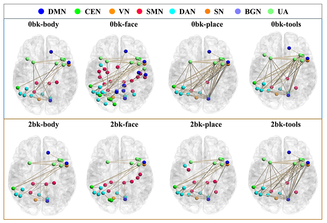
The result of mapping our geometric attention mechanism back to the brain on the testing set for different brain cognitive tasks.

TABLE III.

Contribution Degree of Each Subnetwork for Eight Different Brain Cognitive States

	DMN	SMN	CEN	VN	DAN	SN	BGN	UA
0bk-body	16%	20%	12%	5%	22%	6%	1%	18%
Obk-face	$19\mathrm{\%}$	$22\mathrm{\%}$	$12\mathrm{\%}$	$6\mathrm{\%}$	$19\mathrm{\%}$	$5\mathrm{\%}$	$1\mathrm{\%}$	$16\mathrm{\%}$
0bk-place	$19\mathrm{\%}$	$22\mathrm{\%}$	$13\mathrm{\%}$	$5\mathrm{\%}$	$19\mathrm{\%}$	$6\mathrm{\%}$	$2\mathrm{\%}$	$15\mathrm{\%}$
0bk-tools	$19\mathrm{\%}$	$21\mathrm{\%}$	$13\mathrm{\%}$	$5\mathrm{\%}$	$19\mathrm{\%}$	$5\mathrm{\%}$	$3\mathrm{\%}$	$16\mathrm{\%}$
2bk-body	$17\mathrm{\%}$	$20\mathrm{\%}$	$11\mathrm{\%}$	$6\mathrm{\%}$	$22\mathrm{\%}$	$6\mathrm{\%}$	$3\mathrm{\%}$	$15\mathrm{\%}$
2bk-face	$14\mathrm{\%}$	$24\mathrm{\%}$	$13\mathrm{\%}$	$5\mathrm{\%}$	$20\mathrm{\%}$	$5\mathrm{\%}$	$1\mathrm{\%}$	$18\mathrm{\%}$
2bk-place	$18\mathrm{\%}$	$23\mathrm{\%}$	$11\mathrm{\%}$	$5\mathrm{\%}$	$20\mathrm{\%}$	$5\mathrm{\%}$	$2\mathrm{\%}$	$15\mathrm{\%}$
2bk-tools	$17\mathrm{\%}$	$25\mathrm{\%}$	$11\mathrm{\%}$	$4\mathrm{\%}$	$18\mathrm{\%}$	$5\mathrm{\%}$	$0\mathrm{\%}$	$15\mathrm{\%}$

5). Evaluating the Replicability of Change Detection:

Since each subject has the test-retest fMRI scans where the tasks were performed in a different order, we evaluate the replicability of the detected brain state changes between test and retest data. Take our method as an example, we first train a model on test fMRI data only (called OURNet-1) and another model training on retest fMRI data solely (called OURNet-2). We then apply OURNet-1 on the testing set of test fMRI data (i.e., same task schedule) and retest data (i.e., different task schedule), respectively. Similarly, OURNet-2 also performs the same operation as OURNet-1. Other comparative deepbased methods follow the same training manner. We show the purity score of these methods in Table IV. It is apparent that our geometric attention neural network also has the highest replicability performance compared to other methods in both same and different task scenarios, as the large $p$-values (indicating high test-retest replicability) are shown in Table IV.

TABLE IV.

Replicability Analysis Results

		same task schedule vs. different task schedule			same task schedule vs. different task
OURNet-1	mean±std	0.7596±0.0632 vs. 0.7549±0.0633	OURNet-2	mean±std	0.7594±0.0634 vs. 0.7583±0.0640
	t-test	No significant difference found (p=0.4899)		t-test	No significant difference found (p=0.8238)
SPDNet-1	mean±std	0.7318±0.0497 vs. 0.7286±0.0575	SPDNet-2	mean±std	0.7366±0.0543 vs. 0.7276±0.0514
	t-test	No significant difference found (p=0.4600)		t-test	No significant difference found (p=0.0329)
CPDNet-1	mean±std	0.7417±0.0547 vs. 0.7388±0.0567	CPDNet-2	mean±std	0.7400±0.0545 vs. 0.7387±0.0535
	t-test	No significant difference found (p=0.0781)		t-test	No significant difference found (p=0.7544)
SCGNN-1	mean±std	0.6935±0.0498 vs. 0.6643±0.0537	SCGNN-2	mean±std	0.6770±0.0512 vs. 0.6741±0.0464
	t-test	Significant difference found (p<0.0001)		t-test	No significant difference found (p=0.4523)

6). Ablation Study:

To further verify the contributions of the proposed SPD-CNN and GAM in the underlying neural network framework, we conduct an ablation study conducted on real task-based fMRI data (involved test and retest data). Precisely, we first remove the two components separately, then train the model in turn, and finally test its performance. Table V shows that each component plays an essential role in change detection, as evidenced by the significant difference $p<{10}^{-3}$ after removing either or both components.

TABLE V.

Ablation Study on SPD-CNN and GAM Modules

SPD-CNN		$\times$	$\surd$	$\surd$
GAM		$\times$	$\times$	$\surd$
Purity	Mean	0.6904	0.7490	0.7595
	STD	0.0534	0.0625	0.0632
$t$-test		$p<{10}^{-4}$	$p<{10}^{-3}$	--

7). Discussions:

Overall, through comprehensive experiments on simulated and real data, our geometric-attention neural network shows promising results in detecting brain state changes in terms of accuracy and consistency. Since the Euclidean operations in non-manifold methods might undermine the intrinsic data geometry, the overall performance is generally worse than manifold-based approaches. Learning-based methods usually outperform the non-learning-based methods since the feature representation learning is eventually optimized for the brain state change detection. Since the brain network data is often in a high dimension and noisy, learning the compact representation is important to distinguish the brain states underlying different cognitive tasks. The layer-by-layer learning mechanism in deep neural networks is more effective than the shallow models such as dGE. The geometric attention component makes our method more accurate in detecting brain state changes than current state-of-the-art deep learning methods by focusing on the most relevant parts of the brain network.

Regarding the effect of sliding widow size, most of the change detection methods achieve peak performance at the range of 20-30 time points, as shown in Figure 7. Although the FC matrix using a smaller window size have higher sensitivity to detect the change, the specificity is low. Compared to all other methods, our proposed method is less sensitive to the sliding window size even in the scenario of extremely small and extremely large sizes.

This paper mainly focuses on the change detection on task fMRI data, which has been cast as a supervised learning problem. Herein, we position our work as a new computational method to understand the functional dynamics by investigating the intrinsic geometry of the evolving functional connectivity. Hence, detecting brain states change is just the starting point of the research on learning functional dynamics. In neuroscience and the clinical field, it is more attractive to characterize the functional dynamics in the resting state. As a proof-of-concept work, the backbone pieces of SPD-CNN and MMS-RNN enable the development of the unsupervised learning approach for resting-state fMRI applications.

V. Conclusion

In this work, we propose a novel manifold-based deep learning solution to characterize the dynamics of SPD matrix time series. Specifically, we present a novel SPD-CNN with the geometric attention mechanism to learn the compact manifold feature representation, followed by a manifold-based RNN for characterizing the temporal behavior of SPD matrices. Since the functional brain network is essentially represented by the correlation of neuroimaging data, our proposed manifold solution offers a new window to identify brain state changes using the state-of-the-art machine learning technique. Experimental results on both simulated and real functional neuroimaging data show that our method can achieve more accurate and consistent change detection results than current methods, which indicates the great applicability of our deep learning approach in neuroimaging area. In the future, we will extend our method to resting-state fMRI where our goal is to develop a novel manifold-based connectome biomarker for neurological diseases.

References

- [1].Hu R et al. , “Multi-band brain network analysis for functional neuroimaging biomarker identification,” IEEE Trans. Med. Imag, vol. 40, no. 12, pp. 3843–3855, Dec. 2021. [DOI] [PMC free article] [PubMed] [Google Scholar]
- [2].Yang Z, Dan T, and Yang Y, “Multi-temporal remote sensing image registration using deep convolutional features,” IEEE Access, vol. 6, pp. 38544–38555, 2018. [Google Scholar]
- [3].Sanin A, Sanderson C, Harandi MT, and Lovell BC, “Spatiotemporal covariance descriptors for action and gesture recognition,” in Proc. IEEE Workshop Appl. Comput. Vis. (WACV), Jan. 2013, pp. 103–110. [Google Scholar]
- [4].Huang Z and Gool LV, “A Riemannian network for SPD matrix learning,” presented at the 31st AAAI Conf. Artif. Intell., San Francisco, CA, USA, 2017. [Google Scholar]
- [5].Nguyen XS, Brun L, Lezoray O, and Bougleux S, “A neural network based on SPD manifold learning for skeleton-based hand gesture recognition,” in Proc. IEEE/CVF Conf. Comput. Vis. Pattern Recognit. (CVPR), Jun. 2019, pp. 12028–12037. [Google Scholar]
- [6].Zhang T, Zheng W, Cui Z, and Li C, “Deep manifold-to-manifold transforming network for action recognition,” IEEE Trans. Multimedia, vol. 22, no. 11, pp. 2926–2937, Nov. 2020. [Google Scholar]
- [7].Zhang T, Zheng W, Cui Z, and Li C, “Deep manifold-to-manifold transforming network,” in Proc. 25th IEEE Int. Conf. Image Process. (ICIP), Oct. 2018, pp. 4098–4102. [Google Scholar]
- [8].Sporns O, Networks of the Brain. Cambridge, MA, USA: MIT Press, 2010. [Google Scholar]
- [9].Hutchison RM et al. , “Dynamic functional connectivity: Promise, issues, and interpretations,” Neuroimage, vol. 80, pp. 360–378, Oct. 2013. [DOI] [PMC free article] [PubMed] [Google Scholar]
- [10].Tuzel O, Porikli F, and Meer P, “Pedestrian detection via classification on Riemannian manifolds,” IEEE Trans. Pattern Anal. Mach. Intell, vol. 30, no. 10, pp. 1713–1727, Oct. 2008. [DOI] [PubMed] [Google Scholar]
- [11].Dong Z, Jia S, Zhang C, Pei M, and Wu Y, “Deep manifold learning of symmetric positive definite matrices with application to face recognition,” presented at the 31st AAAI Conf. Artif. Intell., San Francisco, CA, USA, 2017. [Google Scholar]
- [12].Wu Y, Jia Y, Li P, Zhang J, and Yuan J, “Manifold Kernel sparse representation of symmetric positive-definite matrices and its applications,” IEEE Trans. Image Process, vol. 24, no. 11, pp. 3729–3741, Nov. 2015. [DOI] [PubMed] [Google Scholar]
- [13].Lin Y, Hou J, Laurienti PJ, and Wu G, “Detecting changes of functional connectivity by dynamic graph embedding learning,” in Medical Image Computing and Computer Assisted Intervention MICCAI, vol. 12267, Cham, Switzerland: Springer, 2020, pp. 489–497. [Google Scholar]
- [14].Shappell H, Caffo BS, Pekar JJ, and Lindquist MA, “Improved state change estimation in dynamic functional connectivity using hidden semi-Markov models,” NeuroImage, vol. 191, pp. 243–257, May 2019. [DOI] [PMC free article] [PubMed] [Google Scholar]
- [15].Li H and Fan Y, “Identification of temporal transition of functional states using recurrent neural networks from functional MRI,” in Medical Image Computing and Computer Assisted Intervention MICCAI, Cham, Switzerland: Springer, 2018, pp. 232–239. [DOI] [PMC free article] [PubMed] [Google Scholar]
- [16].Arsigny V, Fillard P, Pennec X, and Ayache N, “Geometric means in a novel vector space structure on symmetric positive-definite matrices,” SIAM J. Matrix Anal. Appl, vol. 29, no. 1, pp. 328–347, Jan. 2007. [Google Scholar]
- [17].Huang Z, Wu J, and Van Gool L, “Building deep networks on Grassmann manifolds,” in Proc. AAAI Conf. Artif. Intell., vol. 32, no. 1, 2018, pp. 3279–3286. [Google Scholar]
- [18].Barch DM et al. , “Function in the human connectome: Task-fMRI and individual differences in behavior,” NeuroImage, vol. 80, pp. 169–189, Oct. 2013. [DOI] [PMC free article] [PubMed] [Google Scholar]
- [19].Rodriguez A and Laio A, “Clustering by fast search and find of density peaks,” Science, vol. 344, no. 6191, pp. 1492–1496, 2014. [DOI] [PubMed] [Google Scholar]
- [20].Lin Y et al. , “Learning dynamic graph embeddings for accurate detection of cognitive state changes in functional brain networks,” NeuroImage, vol. 230, Apr. 2021, Art. no. 117791. [DOI] [PMC free article] [PubMed] [Google Scholar]
- [21].Bianchi FM, Grattarola D, and Alippi C, “Spectral clustering with graph neural networks for graph pooling,” in Proc. Int. Conf. Mach. Learn., 2020, pp. 874–883. [Google Scholar]
- [22].Huang Z, Cai H, Dan T, Lin Y, Laurienti P, and Wu G, “Detecting brain state changes by geometric deep learning of functional dynamics on Riemannian manifold,” in Proc. Int. Conf. Med. Image Comput. Comput.-Assist. Intervent, Cham, Switzerland: Springer, 2021, pp. 543–552. [Google Scholar]
- [23].Erhardt EB, Allen EA, Wei Y, Eichele T, and Calhoun VD, “SimTB, a simulation toolbox for fMRI data under a model of spatiotemporal separability,” NeuroImage, vol. 59, pp. 4160–4167, Feb. 2012. [DOI] [PMC free article] [PubMed] [Google Scholar]
- [24].Ting C-M, Ombao H, Samdin SB, and Salleh S-H, “Estimating dynamic connectivity states in fMRI using regime-switching factor models,” IEEE Trans. Med. Imag, vol. 37, no. 4, pp. 1011–1023, Apr. 2018. [DOI] [PubMed] [Google Scholar]
- [25].Glasser MF et al. , “The minimal preprocessing pipelines for the human connectome project,” NeuroImage, vol. 80, pp. 105–124, Oct. 2013. [DOI] [PMC free article] [PubMed] [Google Scholar]
- [26].Pruim RHR, Mennes M, van Rooij D, Llera A, Buitelaar JK, and Beckmann CF, “ICA-AROMA: A robust ICA-based strategy for removing motion artifacts from fMRI data,” NeuroImage, vol. 112, pp. 267–277, May 2015. [DOI] [PubMed] [Google Scholar]
- [27].Pruim RHR, Mennes M, Buitelaar JK, and Beckmann CF, “Evaluation of ICA-AROMA and alternative strategies for motion artifact removal in resting state fMRI,” NeuroImage, vol. 112, pp. 278–287, May 2015. [DOI] [PubMed] [Google Scholar]
- [28].Shen X, Tokoglu F, Papademetris X, and Constable RT, “Groupwise whole-brain parcellation from resting-state fMRI data for network node identification,” NeuroImage, vol. 82, pp. 403–415, Nov. 2013. [DOI] [PMC free article] [PubMed] [Google Scholar]
- [29].Moussa MN, Steen MR, Laurienti PJ, and Hayasaka S, “Consistency of network modules in resting-state fMRI connectome data,” PLoS ONE, vol. 7, no. 8, Aug. 2012, Art. no. e44428. [DOI] [PMC free article] [PubMed] [Google Scholar]
- [30].Newman MEJ and Girvan M, “Finding and evaluating community structure in networks,” Phys. Rev. E, Stat. Phys. Plasmas Fluids Relat. Interdiscip. Top, vol. 69, no. 2, Feb. 2004, Art. no. 026113. [DOI] [PubMed] [Google Scholar]
- [31].Girvan M and Newman ME, “Community structure in social and biological networks,” Proc. Nat. Acad. Sci. USA, vol. 99, no. 12, pp. 7821–7826, Jun. 2002. [DOI] [PMC free article] [PubMed] [Google Scholar]
- [32].Mayhugh RE et al. , “Moderate-heavy alcohol consumption lifestyle in older adults is associated with altered central executive network community structure during cognitive task,” PLOS ONE, vol. 11, no. 8, Aug. 2016, Art. no. e0160214. [DOI] [PMC free article] [PubMed] [Google Scholar]
- [33].Dai C et al. , “Effects of sleep deprivation on working memory: Change in functional connectivity between the dorsal attention, default mode, and fronto-parietal networks,” Frontiers Hum. Neurosci, vol. 14, p. 360, Oct. 2020. [DOI] [PMC free article] [PubMed] [Google Scholar]
- [34].Zhang G, Li Y, and Zhang J, “Tracking the dynamic functional network interactions during goal-directed auditory tasks by brain state clustering,” Frontiers Neurosci, vol. 13, p. 1220, Nov. 2019. [DOI] [PMC free article] [PubMed] [Google Scholar]
- [35].Ting C-M, Ombao H, Samdin SB, and Salleh S-H, “Estimating dynamic connectivity states in fMRI using regime-switching factor models,” IEEE Trans. Med. Imag, vol. 37, no. 4, pp. 1011–1023, Apr. 2018. [DOI] [PubMed] [Google Scholar]