Directed acyclic graphs for clinical research: a tutorial

Abstract

Directed acyclic graphs (DAGs) are useful tools for visualizing the hypothesized causal structures in an intuitive way and selecting relevant confounders in causal inference. However, in spite of their increasing use in clinical and surgical research, the causal graphs might also be misused by a lack of understanding of the central principles. In this article, we aim to introduce the basic terminology and fundamental rules of DAGs, and DAGitty, a user-friendly program that easily displays DAGs. Specifically, we describe how to determine variables that should or should not be adjusted based on the backdoor criterion with examples. In addition, the occurrence of the various types of biases is discussed with caveats, including the problem caused by the traditional approach using p-values for confounder selection. Moreover, a detailed guide to DAGitty is provided with practical examples regarding minimally invasive surgery. Essentially, the primary benefit of DAGs is to aid researchers in clarifying the research questions and the corresponding designs based on the domain knowledge. With these strengths, we propose that the use of DAGs may contribute to rigorous research designs, and lead to transparency and reproducibility in research on minimally invasive surgery.

INTRODUCTION

In medical research, causality has been dealt with as one of the utmost importance. For instance, studies regarding minimally invasive surgery (MIS) are based on the causal hypothesis that such a surgical method will reduce the burden on patients and lead to a decrease in morbidity and rapid functional recovery compared to conventional open surgical treatments [1,2]. However, randomized controlled trials, considered as the gold standard for causality [3–5], are often difficult to implement owing to ethical or economic issues. For these reasons, researchers frequently conduct observational studies, but these are often regarded as providing association results, not causality [3,4]. The main reason for losing causal meaning is the failure to compare like with like. For example, various baseline characteristics such as age and socioeconomic status may not be balanced between the two groups. To make them comparable, confounders should be cautiously adjusted to identify the causal effect of interest. Nonetheless, it is a difficult task to determine which variables to adjust or not to adjust in observational studies. Traditional variable selection methods such as backward elimination and stepwise selection have been criticized because they often lead to biased causal effect estimates. Other variable selection methods are also subject to the same criticism. In particular, variable selection for prediction purposes may not be optimal for causal inference.

For variable selection with a focus on causal inference, we should determine which variables confound the relationship between the treatment (or exposure) variable and the outcome variable of interest. For this understanding, we need domain knowledge about the causal structure among the research variables. Directed acyclic graphs (DAGs) [4,7–9] have been widely used to visualize the domain knowledge, show which variables are confounders to be adjusted, and indicate when the causal effect of interest is nonparametrically identified in observational studies. Moreover, DAGs aid researchers in clarifying possible biases from current research designs such as selection bias and measurement error bias. Consequently, the use of DAGs may contribute to transparency and reproducibility in surgical research. In fact, a growing number of clinical journals have requested their inclusion in either the main body or supplementary material. Notwithstanding their recent extensive use, however, the lack of a clear understanding of the essential principles of DAGs may lead to their incorrect use [10].

In this article, we aim to describe the fundamental principles of DAGs and highlight their strengths in surgical research using practical examples. For this purpose, the current paper consists of the following three steps. In the first step, we briefly review the basic concepts and rules of DAGs. Especially, we link them to clinical examples from the literature on MIS. In the next step, we demonstrate potential pitfalls caused by the traditional p-value–based approach for confounder selection and emphasize the importance of theory-based DAGs in empirical studies. In the final step, we demonstrate DAGitty, a user-friendly program for displaying DAGs, with practical examples. These examples are used to illustrate caveats and recommendations for using DAGs in surgical research.

BASIC TERMINOLOGY AND FUNDAMENTAL PRINCIPLES OF DIRECTED ACYCLIC GRAPHS

In this section, we briefly review the basic concepts and terminologies pertaining to DAGs and introduce important criteria that help readers specify research models.

Basic terminology: what are directed acyclic graphs?

Mathematically, a graph is defined as a set of nodes and edges. In a graph, nodes may or may not be connected by edges. DAGs additionally have two important characteristics. First, a directed graph is a graph whose every edge has a direction [9]. Second, an acyclic graph contains no directed cycles [9]. An example of cyclic graphs is X → Y → Z → X, because X returns to itself. DAGs rule out graphs with such a cyclic loop. We interchangeably use the term arrow with directed edges throughout this paper. In DAGs, an arrow represents a (possibly non-zero) causal effect. Especially, in DAGs, to interpret arrows as causal relations, all common causes of any pair of variables on the graph should be incorporated [11].

We consider simple examples of DAGs for explanatory purposes. In Fig. 1A, we see the arrow from X to Y, which means that X may or may not affect Y. In contrast, in Fig. 1B, it is assumed that X does not affect Y based on the absence of the arrow. The third graph depicted in Fig. 1C, the simplest one among the three graphs, represents not only the possible causal relationships between X and Y but also the absence of common causes such as L in the other graphs.

Fig. 1.

(A) A directed acyclic graph (DAG) indicating the causal relation between X and Y with a common cause (L). (B) A DAG indicating the null causal relation between X and Y with a common cause (L). (C) A DAG indicating the causal relation between X and Y in the absence of a common cause.

It is worth mentioning that we do not assume any functional form for the causal relationship [7–9]. In a nutshell, an arrow from X to Y represents our hypothesized causal direction between two variables but does not contain any information about its detailed functional form, e.g., linear, quadratic, or logarithm.

To deal with causal relationships generally, it is useful to categorize nodes as shown below. Consider first Fig. 2. We see that the graph consists of four nodes with three arrows. In this graph, the node where the arrow starts from L is called the parent of the node that the edge goes into X. In a similar manner, the node that the edge goes into is defined as the child of the node it comes from [4,9]. Therefore, Fig. 2 suggests that L is the parent of X, X is the parent of Y, and Y is the parent of Z. This means that L is connected to Z through X and Y, which is called the path between L and Z. In graphs including more nodes, there are many parents and children. If two nodes are connected by a directed path, the starting node is called the ancestor of all nodes on the corresponding path, and the other nodes are called the descendants of the ancestor. For instance, it is clear that L is the ancestor of X, Y, and Z, and Z is the descendant of L, X, and Y in Fig. 2. Furthermore, it is worth mentioning that an ancestor cannot be its descendant because we deal with graphs without cycles.

Fig. 2.

An example of a path.

The key information of DAGs lies in the absence of the arrow and its direction because they represent the causal structure of research variables based on subject matter knowledge. We introduce three fundamental configurations that constitute the basis of the general forms of DAGs. These consist of three nodes and two arrows. The first configuration is a chain, which has an arrow coming into the middle node and another arrow coming out of the middle node [9]. To put it another way, a chain has only one-way arrows. In Fig. 3, we can imagine that the flow of water going from A to C can be blocked by using B. This can be translated as A and C are conditionally independent given B. To help readers understand this concept, consider that A is gender, B is occupation, and C is asbestos exposure. In this chain, A affects C because the majority of people who work at construction sites dealing with asbestos are men. However, gender may not affect asbestos exposure within each type of occupation. This is what conditional independence means. In mathematical language, conditional independence of the chain is expressed as A ⊥ C | B.

Fig. 3.

An example of a chain. A, gender; B, occupation; C, asbestos exposure.

The second configuration is called a fork, which includes two arrows stemming from the middle node [9]. An example of a fork is suggested in Fig. 4, where B is a common cause of C and D. In the fork. if the middle node (B in Fig. 4) is given, the other two nodes (C and D) are independent. For example, we construct a model for workers using Fig. 4 including three variables (B, occupation; C, asbestos exposure; and D, smoking). In this case, workers in some occupations have a higher or lower tendency to smoke, and types of occupation are related to asbestos exposure. However, if we observe workers within each occupation, we will not find evidence that smoking affects asbestos exposure or vice versa. This case is mathematically represented as C ⊥ D | B.

Fig. 4.

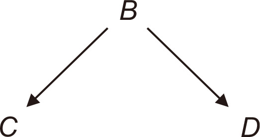
An example of a fork. B, occupation; C, asbestos exposure; D, smoking.

A collider, the third configuration, denotes the middle node into which two arrows are directed [9]. In Fig. 5, C and D are unconditionally independent. The imaginary flow of water going from C to E as well as going from D to E is blocked without using E because the flow from C to E collides with the flow from D to E. What if we condition on the collision node, E, instead? In this situation, C and D are generally dependent. To comprehend the failure of conditional independence when the collider node is conditioned, it would be helpful to look at the following example. Suppose there is a theoretical hypothesis that smoking or asbestos exposure causes lung cancer in men (assuming no other factors). In this case, we assume that there are only two causes of lung cancer and the causes are independent. If we evaluated a lung cancer patient and found that he was a nonsmoker, we would conclude that he developed lung cancer due to asbestos exposure with high probability. This explains why conditional independence does not hold when the collision node is given. Furthermore, conditional independence also does not hold if not only E is conditioned but also its descendants are conditioned, provided that the descendants of E exist. In Fig. 5, the corresponding mathematical expressions are written as C ⊥ D and C ⊥⁄ D | E .

Fig. 5.

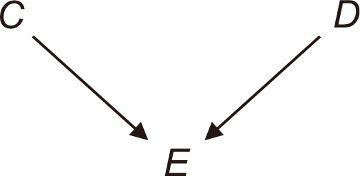
An example of a collider. C, asbestos exposure; D, smoking; E, lung cancer in men.

We introduced some basic and important components of DAGs and how to connect (unconditional and conditional) independence with simple DAG structures. Nonetheless, DAGs used in actual research are not as simple as the examples suggested above. To determine conditional independence among variables in general, the following rule, d-separation (d means directional), provides a general principle based on the aforementioned rules [4,8,9].

Definition 1 (d-separation)

A path p is blocked by a set of nodes N if and only if

1. p contains a chain or fork such that the middle node is in N, or

2. p contains a collider such that the collision node and its descendants are not in N.

As can be seen, these two rules are already mentioned in the previous examples. If a pair of nodes is d-separated, they are conditionally independent. From the perspective of graphs, it means that every path between the nodes is blocked. If two nodes are not d-separated, they are called d-connected.

Fig. 6 shows a DAG including chains, forks, and colliders. In the causal diagram, the path between A and B is d-separated if any other nodes are not given. How about the path between C and D? They are d-connected, because they share a common cause, A. Note that they are independent, conditioned on A. In addition, suppose that F is also given. In this case, they are not independent anymore because the descendant F of the collision node E is given. As a final example, we look at the paths between A and G (A → D → E → F ← G, and A → C → E → F ← G). It seems obvious that the two nodes are unconditionally independent. In contrast, they are not generally independent if F is given.

Fig. 6.

An example of directed acyclic graphs including chains, forks, and colliders.

Confounding and the backdoor criterion

Although it is widely recognized that confounding should be considered properly in research designs, it is not easy to decide which variables should be adjusted in each study. DAGs can help researchers to identify them. The intuition behind the variable selection based on DAGs is that we block non-causal paths (the so-called backdoor paths) and keep causal paths of interest open [4,9]. As can be seen in Fig. 7A, the graph includes a fork representing X and Y sharing a common cause L. In this situation, suppose that we adjust L which lies in a non-causal path from X to Y. The adjustment of L is depicted by a box around the variable in the graph on the right, and the adjustment of a common cause eliminates the dependence between its children X and Y. If we perform a statistical analysis without taking into account L in this case, the resulting estimate would be biased owing to confounding bias [12].

Fig. 7.

(A) An open backdoor path without the adjustment of L. (B) A blocked backdoor path with the adjustment of L.

Should we adjust L in Fig. 8? Generally, not if a researcher is interested in the causal effect from X on Y. If we adjust L, which is called a mediator in the literature of mediation analysis, it eliminates the effect of X on Y through L. Noting that Fig. 8 implies that L may have a statistically significant association with Y, we should not include all (possibly) associated variables, and that is why we should focus on the causal structure of research variables.

Fig. 8.

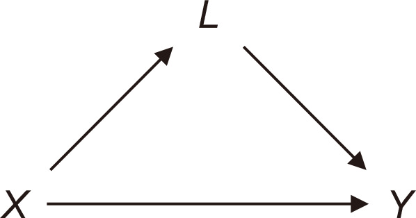
An example of directed acyclic graph with a mediator.

When researchers carry out observational studies, there may be cases where some variables are omitted or not measured owing to reasons such as protection of personal information or difficulty of measurement. If the nodes are not all present in a DAG, is it possible to investigate the causal effect in this situation? Fortunately, it is still possible in many cases. More precisely, there is a general condition to estimate the effect of X on Y, and the so-called backdoor criterion [8,9], helps researchers make the decision.

Definition 2 (the backdoor criterion)

Given an ordered pair of variables (X,Y) in a DAG, a set of variables S satisfies the backdoor criterion relative to (X,Y) if no node in S is a descendant of X, and S blocks every path between X and Y that contains an arrow into X.

For a more concrete explanation, we revisit the example described in Fig. 6. Suppose that our aim is to investigate the causal effect of C on F. The backdoor criterion tells us that every backdoor path should be blocked by a set of variables excluding descendants of C. As A and G are ancestors of C, a set S satisfying definition 2 is S = {A, G}, and the following backdoor paths become blocked.

C ← A → D → E → F, C ← A → D → F, C ← G → F

An important question is to ask whether such S is unique. The answer is generally no. Suppose that A is not included in the data, whereas the causal structure remains the same. In this case, it is obvious that the two paths including A are open, and the corresponding confounding bias consequently occurs. However, there is another way to block the non-causal paths: to control for D and G instead. In this regard, the backdoor criterion provides us with alternatives to estimate the causal effect even if some of the confounders (i.e., A) are unobserved. In addition, some readers might notice that there are more candidates for S. For example, the union of {A, G} and {D, G} also satisfies definition 2. The sets {A, G}, {D, G}, {A, D, G}, {A, B, G}, {B, D, G}, and {A, B, D, G} are candidates for S. Among these sets, the smallest sets, {A, G} and {D, G}, are called the minimally sufficient adjustment sets [7,13].

DIRECTED ACYCLIC GRAPHS’ WARNING AGAINST CONFOUNDER SELECTION USING p-VALUES

In practice, researchers conventionally select confounders based on the statistical significance using p-values [14–16]. However, using p-values for the variable selection without understanding the causal structure may considerably distort the causal effect of interest. For a concrete explanation, consider Fig. 9 by Liu et al. [17] showing a hypothesized causal model including five binary variables (depression [DEP], ever smoker [SMOKE], coronary artery disease [CAD], selective serotonin reuptake inhibitor [SSRI], lung cancer [L-CANCER]).

Fig. 9.

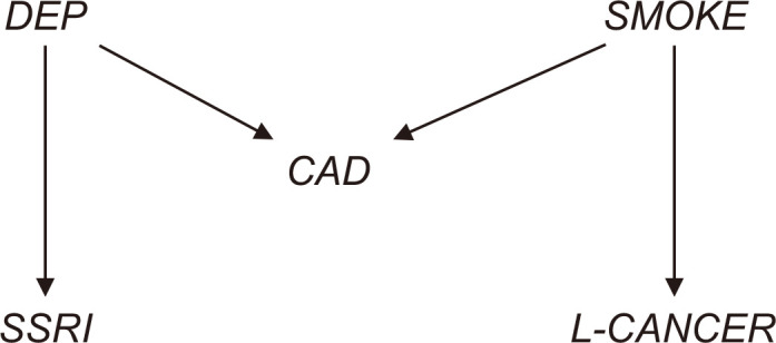
An example of M-bias. DEP, depression; SMOKE, ever smoker; CAD, coronary artery disease; SSRI, selective serotonin reuptake inhibitor; L-CANCER, lung cancer.

For the moment, assume that we collect data without DEP and SMOKE. The causal relationship of our interest is the relationship between SSRI and L-CANCER. In this situation, the traditional confounder selection strategy using p-values will include CAD as a confounder. However, the DAG clearly indicates that DEP is a parent of CAD and SSRI, and SMOKE causes CAD and L-CANCER (two forks), and CAD is the common descendant of DEP and SMOKE (one collider). As a result, SSRI and L-CANCER are unconditionally independent. In this situation, a collider bias can occur if CAD is adjusted. That is, the decision to include the collision node as a confounder based on p-values may induce bias by opening the non-causal path between two variables. Table 1 shows a numerical result of the consequence of this defective strategy.

Table 1.

Simulation result for Liu et al. [17]

	RR	% Bias
Incorrect model	0.979	–2.085
Correct model	1.000	<0.001

RR, relative risk (the true RR is 1).

For this numerical study, Poisson regression was used and relative risks (RR) were reported. In Table 1, the estimated RR (0.979) is reported as the average of 1,000 estimates obtained by each generated data set, and the bias presents the difference between RR and the true value of 1. The result indicates that the bias of RR obtained by the model adjusting CAD (incorrect model) is much larger than that of the model without CAD (correct model). This is called M-bias [18], named after the shape of the graph presented above. The example of M-bias demonstrates that adjustment of variables associated with both exposure and outcome may be even harmful. This example is particularly appealing to explain why we should clearly understand causal structures. Another example of M-bias is provided by [18], and related discussions are suggested in [17,19,20].

It is important to note that satisfying the backdoor criterion in DAGs refers to no unmeasured confounding assumption or conditional exchangeability mentioned in causal inference. Statistical methods used in causal inference such as standardization, inverse probability of treatment weighting, and matching with propensity score are valid when no unmeasured confounding assumption or conditional exchangeability assumption holds. A set of variables W for satisfying the backdoor criterion in a DAG satisfies no unmeasured confounding assumption or conditional exchangeability assumption. In this respect, the strength of DAGs evidently appears in that they provide detailed information about confounder selection and identification of the causal effects for each hypothesized causal structure. As described in the previous examples, DAGs display not only variables to be adjusted but also variables not to be adjusted. Once we specify the set of confounders to be adjusted, researchers should determine some parametric or functional forms of confounders in the propensity score model or outcome regression model. In this case, p-values can be utilized in practice. Alternatively, various machine learning techniques allowing a wide range of functional forms can be applied [21–23].

A GUIDE TO USE DAGitty WITH EXAMPLES

Even though we have explained the fundamental rules such as d-separation and the backdoor criterion, it is fairly difficult for researchers to apply those rules to their own DAGs and determine which variables should be adjusted. DAGitty is a useful tool that helps researchers specify the set of variables to be adjusted in complex situations, and its web user interface version is available at http://www.DAGitty.net/dags.html.

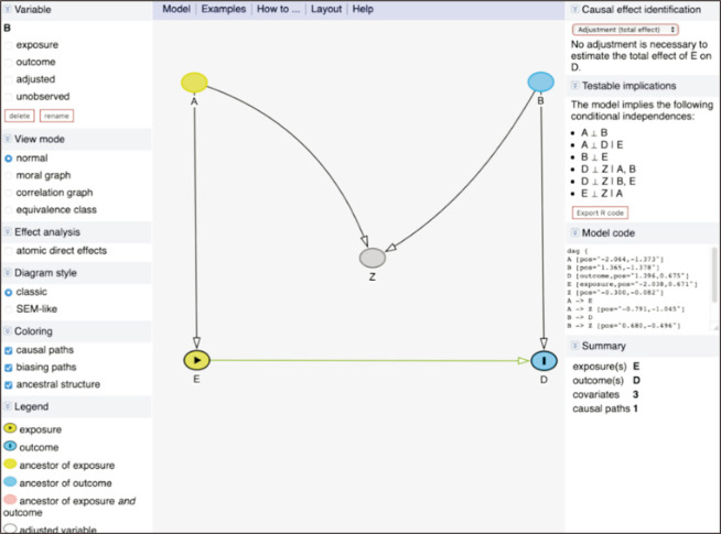
When users access the website, Fig. 10 shows what is displayed on the screen. A new node is generated by clicking on an empty spot on the graph and typing a variable name. In addition, a directed arrow between two nodes can be inserted by clicking the ancestor node first and then the other node. If you click once more on the ancestor node, the arrow is deleted. On the left side, menus for basic operations are displayed. We focus on the essential ones for beginners. The first menu on the left shows Variables, which contain four categories: exposure, outcome, adjusted, and unobserved. The third category adjusted means variables that are adjusted in the analysis, and the remaining category unobserved refers to variables that are not included in the data. In addition, users can eliminate the names of variables by pressing delete and change variable names using rename. Next, Legend at the bottom of the menu provides the meaning of each element in the currently represented graph. In particular, it clearly suggests the ancestors of the exposure and outcome. More importantly, unobserved confounders and what path biases occur by not adjusting them can be identified. Biasing paths are displayed as violet-colored lines, whereas causal paths are colored green in the graph. If you turn off ancestral structure by clicking on it, detailed information about the ancestor of exposure or outcome is hidden. If some biasing paths remain after users have adjusted available variables, the implemented adjustment is indicated as insufficient and suggests that biases are still present.

Fig. 10.

The default screen and basic interface of DAGitty (http://www.DAGitty.net/dags.html).

Causal effect identification at the top on the right directly tells users what variables need to be adjusted to identify the causal effect. The menu below, Testable implications, shows unconditional and conditional independence implied by the current DAG displayed on users’ screens. Model code represents the R-code that can restore the identical result. The figure can be saved as PDF, PNG, or JPEG file in the Model located at the top of the graph. Detailed information about the manipulation of DAGs is provided in [24].

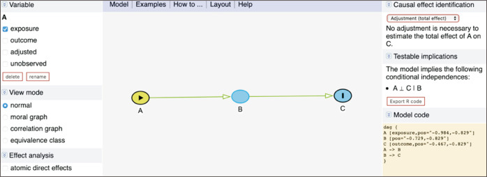
The simple examples illustrated in the previous section are revisited with DAGitty. First, Fig. 11 shows a chain structure. As expected, we see that A and C are independent conditional on B in the testable implications. When we set A as the exposure and C as the outcome in the left-side menu, Causal effect identification informs us that no adjustment is necessary to estimate the causal effect of A on C (A ⊥ C | B).

Fig. 11.

An example of a chain in DAGitty (http://www.DAGitty.net/dags.html). A, gender; B, occupation; C, asbestos exposure.

Fig. 12 represents a fork. The violet-colored biasing path between C and D through B shows that C and D are not unconditionally independent. As explained above, this results from the presence of B, the common cause (also called the ancestor) of C and D. C and D are independent if B is adjusted as shown in the testable implications.

An example of a fork in DAGitty (http://www.DAGitty.net/dags.html). B, occupation; C, asbestos exposure; D, smoking.

Fig. 13 presents the collider case and C and D are unconditionally independent, as displayed in the testable implications (C ⊥ D). However, a biasing path occurs if the state of E is relocated to adjusted in the menu. Indeed, this operation is equivalent to opening the path from C to D by controlling for the collision node, E.

Fig. 13.

An example of a collider in DAGitty (http://www.DAGitty.net/dags.html). C, asbestos exposure; D, smoking; E, lung cancer in men.

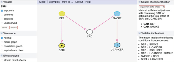
Next, the example of M-bias suggested in Fig. 14, which consists of five variables (DEP, SMOKE, CAD, SSRI, L-CANCER), is revisited. Assuming that we are interested in the causal relationship between SSRI and L-CANCER, they are unconditionally independent, and no adjustment is required as suggested in Causal effect identification. However, the adjustment of CAD induces a bias, because the variable is the collision node and the path from SSRI to L-CANCER becomes open. Therefore, to avoid this collision bias, we need to additionally adjust either DEP or SMOKE.

Fig. 14.

An example including M-bias in DAGitty (http://www.DAGitty.net/dags.html). DEP, depression; SMOKE, ever smoker; CAD, coronary artery disease; SSRI, selective serotonin reuptake inhibitor; L-CANCER, lung cancer.

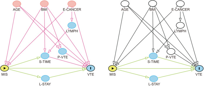
DAGitty has been used in several studies regarding MIS, and we explore an example from [25]. The authors were interested in the causal effect of surgery methods (open vs. MIS) on venous thromboembolism (VTE), and their hypothesized causal structure including nine variables is represented in Fig. 15 using DAGitty.

Fig. 15.

(A) Directed acyclic graph (DAG) before the adjustment. (B) DAG after the adjustment. MIS, minimally invasive surgery; VTE, venous thromboembolism; AGE, patients’ age; BMI, patients’ body mass index; E-CANCER, endometrial cancer; LYMPH, lymphadenectomy; S-TIME, surgical time; L-STAY, length of hospital stay; P-VTE, previous venous thromboembolism.

In the graph, there are three exogenous research variables that are not affected by other variables in the model: patients’ age (AGE), patients’ body mass index (BMI), and endometrial cancer (E-CANCER). The graph on the left suggests a model with no adjustment, and that on the right displays when the five uncolored variables are adjusted. As can be seen, the causal paths of MIS on VTE are colored green in both graphs. However, there are biasing paths colored violet in the unadjusted graph on the left, which means the adjustments are necessary. In particular, the path from surgical time (S-TIME) to VTE is shown as a biasing path compared to the figure on the right.

In this situation, Causal effect identification on the right menu (Fig. 16) helps researchers to correctly adjust confounders. The menu shows that AGE, BMI, and E-CANCER are sufficient for blocking the backdoors paths. It is also possible to adjust previous venous thromboembolism (P-VTE) because the path from P-VTE to VTE is merely blocked and identification of the causal effect would not change. In the original paper, the authors decided to adjust five variables including the three common ancestors of MIS and VTE, and this suggestion reflects their preference to provide a reliable result.

Fig. 16.

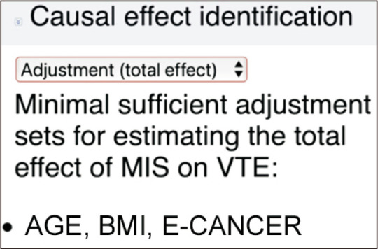
Causal effect identification of the directed acyclic graph in Fig. 15. MIS, minimally invasive surgery; VTE, venous thromboembolism; AGE, patients’ age; BMI, patients’ body mass index; E-CANCER, endometrial cancer.

Then, what if we adjust S-TIME or length of hospital stay (L-STAY), instead? When we attempt to adjust either of them, the following message “The total effect cannot be estimated due to adjustment for an intermediate or a descendant of an intermediate.” appears. This indicates that users tried to control for the variable that lies in a causal path, and this adjustment is not appropriate for estimating the total causal effect of MIS on VTE. Here, intermediate variables in the message refer to mediators.

A PRACTICAL EXAMPLE USING DAGitty IN SURGICAL RESEARCH

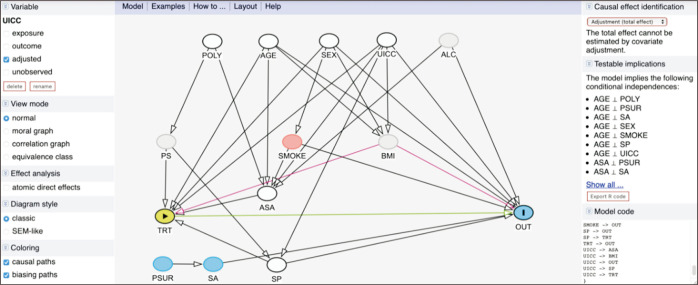
In this section, we present a realistic example of DAG from [26]. Their DAG included 14 variables as shown in Fig. 17. In their study, the intervention was defined as screening for modifiable high-risk factors combined with targeted interventions, and the outcome was postoperative complications in patients undergoing colorectal cancer surgery. Unlike previous examples, the DAG in Fig. 17 included unobserved variables colored gray: ALC, BMI, and PS. Therefore, it is important to ask what the consequences of the unobserved variables on the causal effect of TRT on OUT are.

Fig. 17.

The directed acyclic graph by Bojesen et al. [26]. UICC, Union for International Cancer Control; POLY, polypharmacy; AGE, age; SEX, patients’ sex; ALC, alcohol; PS, union for international cancer control; SMOKE, smoking; BMI, body mass index; TRT, screening for modifiable high-risk factors combined with targeted interventions; ASA, American Society of Anesthesiologists; PSUR, previous surgery; SA, surgical approach; SP, surgical procedure; OUT, postoperative complications in patients undergoing colorectal cancer surgery.

To answer the question, assume that we observed all variables for the moment. In this case, DAGitty suggests three minimal sufficient adjustment sets as shown in Fig. 18. Note that the parents of both TRT and OUT (AGE, BMI, SEX, SP, UICC) are common in all the adjustment sets. The remaining two variables in each set (ALC, SMOKE or ASA, POLY or ASA, PS) indicate different ways to block the remaining backdoor paths. As an example, the second adjustment set S = {AGE, ASA, BMI, POLY, SEX, SP, UICC} is used for estimating the propensity score e = Pr(TRT = 1 | S).

Fig. 18.

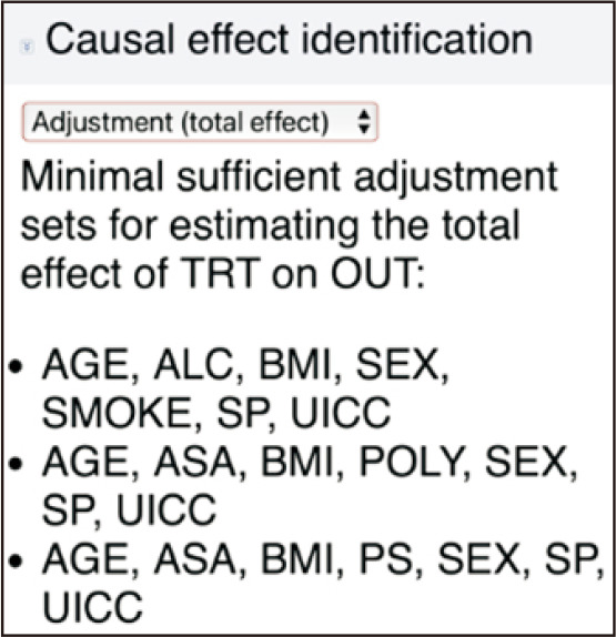
Minimal sufficient adjustment sets in the example of Bojesen et al. [26]. TRT, screening for modifiable high-risk factors combined with targeted interventions; OUT, postoperative complications in patients undergoing colorectal cancer surgery; AGE, age; ALC, alcohol; BMI, body mass index; SEX, patients’ sex; SMOKE, smoking; SP, surgical procedure; UICC, Union for International Cancer Control; ASA, American Society of Anesthesiologists; POLY, polypharmacy; PS, union for international cancer control.

Specifically, the following logistic regression can be used for estimating the propensity score.

However, some variables (ALC, BMI, PS) were not observed in the original paper. It can be seen that the first and third minimal sufficient adjustment sets include two unobserved variables, whereas the second set has one unmeasured variable. Therefore, the causal effect of TRT is not estimable regardless of the choice of the minimal sufficient adjustment sets owing to the unobserved variable. Using the second adjustment set, the presence of a biasing path from BMI can be seen in Fig. 17. The estimate we would obtain from the use of the second adjustment set suffers from the unmeasured confounding bias owing to BMI so that the result should be interpreted with utmost care.

The usefulness of DAG is often beyond selecting confounders. If the DAG were displayed prior to data collection and used in research design, readers might recognize the necessity of BMI to identify the causal effect. In addition, as shown in this example, researchers would notice that not all of the three unobserved variables are prerequisites for the causal effect using DAGs. Consequently, this can lead to focusing on the measurement of the essential variables increasing the feasibility of the research.

CONCLUSION

In this article, the basic terminology and rules of DAGs were introduced. In addition, we focused on how the fundamental concepts and principles such as d-separation and the backdoor criterion are applied to DAGs. Ignoring the causal structure among variables, which corresponds to not using DAGs, in data analysis can lead to various types of biases and causally uninterpretable estimates.

Specifically, the strength of DAGs lies in providing researchers with what they must do and what they must not do based on the hypothesized causal structures. For the former, we emphasized that it is critical to select confounders that block all the backdoor paths, and failure to include them may lead to the unmeasured confounding bias. For the latter, we also illustrated that non–principle-based adjustments of variables can hinder the estimation of the causal effect. In particular, the collider bias and M-bias were described with the examples. Moreover, it was demonstrated that the traditional approach using p-value for confounder selection may be even deleterious to causal inference.

Nonetheless, DAGs also have limitations despite their usefulness and applicability in empirical studies. First, DAGs do not contain information about the functional forms of variables [27]. As shown in the previous examples, the graphs do not assume specific functions such as linear or quadratic. This indicates that researchers should avoid misspecifying the functional forms even with properly selected confounders using DAGs. Therefore, researchers may modify the models based on statistical significance, or employ various machine learning methods that allow a wide range of functional forms. Second, although the various types of biases using DAGs were addressed, their magnitudes are not provided by the graphs themselves [5,27,28]. This implies that additional domain knowledge is required to evaluate the extent of the bias. Third, the causal directions in DAGs are not always clear even when based on theory. In fact, there may be cases where the directions of arrows are somewhat ambiguous, especially when both directions are reasonable. This leads to several different graphs on the same research problem [27,28]. In particular, this issue may arise as the number of variables increases. Concerning this issue, the disjunctive cause criterion was suggested as one of the alternative strategies for confounder selection [16,29]. The criterion states that a sufficient control for confounding is obtained by (1) adjusting all causes of the treatment (exposure), outcome, or both, (2) excluding instrumental variables, and (3) including proxy variables for unmeasured variables that are common causes of treatment and outcome [16]. These practical rules may help researchers select confounders and reduce the risk of unmeasured confounding even when the number of variables is large.

Despite these limitations, DAGs play a major role in shaping research questions and are useful in a priori confounder selection. In this regard, we propose that DAGs should be used frequently in research on MIS for exploring causality. Furthermore, the causal graphs also serve as a useful communication tool for research collaboration in that they clearly convey the hypothesized models to other researchers in an intuitive way.

REFERENCES

- 1.Nezhat F. Minimally invasive surgery in gynecologic oncology: laparoscopy versus robotics. Gynecol Oncol. 2008;111(2 Suppl):S29–S32. doi: 10.1016/j.ygyno.2008.07.025. [DOI] [PubMed] [Google Scholar]
- 2.McAfee PC, Phillips FM, Andersson G, et al. Minimally invasive spine surgery. Spine (Phila Pa 1976) 2010;35(26 Suppl):S271–S273. doi: 10.1097/BRS.0b013e31820250a2. [DOI] [PubMed] [Google Scholar]
- 3.Hernán MA. A definition of causal effect for epidemiological research. J Epidemiol Community Health. 2004;58:265–271. doi: 10.1136/jech.2002.006361. [DOI] [PMC free article] [PubMed] [Google Scholar]
- 4.Pearl J, Glymour M, Jewell NP. Causal inference in statistics: a primer. John Wiley & Sons; 2016. [DOI] [Google Scholar]
- 5.Etminan M, Collins GS, Mansournia MA. Using causal diagrams to improve the design and interpretation of medical research. Chest. 2020;158(1S):S21–S28. doi: 10.1016/j.chest.2020.03.011. [DOI] [PubMed] [Google Scholar]
- 6.Tennant PWG, Murray EJ, Arnold KF, et al. Use of directed acyclic graphs (DAGs) to identify confounders in applied health research: review and recommendations. Int J Epidemiol. 2021;50:620–632. doi: 10.1093/ije/dyaa213. [DOI] [PMC free article] [PubMed] [Google Scholar]
- 7.Greenland S, Pearl J, Robins JM. Causal diagrams for epidemiologic research. Epidemiology. 1999;10:37–48. doi: 10.1097/00001648-199901000-00008. [DOI] [PubMed] [Google Scholar]
- 8.Pearl J. Causal diagrams for empirical research. Biometrika. 1995;82:669–688. doi: 10.1093/biomet/82.4.669. [DOI] [Google Scholar]
- 9.Pearl J. Causality. Cambridge University Press; 2009. [DOI] [Google Scholar]
- 10.Suzuki E, Shinozaki T, Yamamoto E. Causal diagrams: pitfalls and tips. J Epidemiol. 2020;30:153–162. doi: 10.2188/jea.JE20190192. [DOI] [PMC free article] [PubMed] [Google Scholar]
- 11.VanderWeele TJ, Robins JM. Directed acyclic graphs, sufficient causes, and the properties of conditioning on a common effect. Am J Epidemiol. 2007;166:1096–1104. doi: 10.1093/aje/kwm179. [DOI] [PubMed] [Google Scholar]
- 12.VanderWeele TJ, Hernán MA, Robins JM. Causal directed acyclic graphs and the direction of unmeasured confounding bias. Epidemiology. 2008;19:720–728. doi: 10.1097/EDE.0b013e3181810e29. [DOI] [PMC free article] [PubMed] [Google Scholar]
- 13.Greenland S, Pearl J. Article on causal diagrams. In: Boslaugh S, editor. Encyclopedia of epidemiology. Sage Publications; 2007. pp. 149–156. [Google Scholar]
- 14.Sauer BC, Brookhart MA, Roy J, VanderWeele T. A review of covariate selection for non-experimental comparative effectiveness research. Pharmacoepidemiol Drug Saf. 2013;22:1139–1145. doi: 10.1002/pds.3506. [DOI] [PMC free article] [PubMed] [Google Scholar]
- 15.Greenland S, Pearce N. Statistical foundations for model-based adjustments. Annu Rev Public Health. 2015;36:89–108. doi: 10.1146/annurev-publhealth-031914-122559. [DOI] [PubMed] [Google Scholar]
- 16.VanderWeele TJ. Principles of confounder selection. Eur J Epidemiol. 2019;34:211–219. doi: 10.1007/s10654-019-00494-6. [DOI] [PMC free article] [PubMed] [Google Scholar]
- 17.Liu W, Brookhart MA, Schneeweiss S, Mi X, Setoguchi S. Implications of M bias in epidemiologic studies: a simulation study. Am J Epidemiol. 2012;176:938–948. doi: 10.1093/aje/kws165. [DOI] [PubMed] [Google Scholar]
- 18.Rothman KJ, Greenland S, Lash TL. Modern epidemiology. Lippincott Williams & Wilkins; 2008. [DOI] [Google Scholar]
- 19.Greenland S. Quantifying biases in causal models: classical confounding vs collider-stratification bias. Epidemiology. 2003;14:300–306. doi: 10.1097/01.EDE.0000042804.12056.6C. [DOI] [PubMed] [Google Scholar]
- 20.Ding P, Miratrix LW. To adjust or not to adjust? Sensitivity analysis of M-bias and butterfly-bias. J Causal Inference. 2015;3:41–57. doi: 10.1515/jci-2013-0021. [DOI] [Google Scholar]
- 21.Lee BK, Lessler J, Stuart EA. Improving propensity score weighting using machine learning. Stat Med. 2010;29:337–346. doi: 10.1002/sim.3782. [DOI] [PMC free article] [PubMed] [Google Scholar]
- 22.Westreich D, Lessler J, Funk MJ. Propensity score estimation: neural networks, support vector machines, decision trees (CART), and meta-classifiers as alternatives to logistic regression. J Clin Epidemiol. 2010;63:826–833. doi: 10.1016/j.jclinepi.2009.11.020. [DOI] [PMC free article] [PubMed] [Google Scholar]
- 23.Cannas M, Arpino B. A comparison of machine learning algorithms and covariate balance measures for propensity score matching and weighting. Biom J. 2019;61:1049–1072. doi: 10.1002/bimj.201800132. [DOI] [PubMed] [Google Scholar]
- 24.Textor J. Drawing and analyzing causal DAGs with DAGitty. 2015 Aug 19; doi: 10.48550/arXiv.1508.04633. [Preprint]. DOI: https://doi.org/10.48550/arXiv.1508.04633 . [DOI] [Google Scholar]
- 25.Kahr HS, Christiansen OB, Høgdall C, et al. Endometrial cancer does not increase the 30-day risk of venous thromboembolism following hysterectomy compared to benign disease: a Danish National Cohort Study. Gynecol Oncol. 2019;155:112–118. doi: 10.1016/j.ygyno.2019.07.022. [DOI] [PubMed] [Google Scholar]
- 26.Bojesen RD, Grube C, Buzquurz F, Miedzianogora RE, Eriksen JR, Gögenur I. Effect of modifying high-risk factors and prehabilitation on the outcomes of colorectal cancer surgery: controlled before and after study. BJS Open. 2022;6:zrac029. doi: 10.1093/bjsopen/zrac029. [DOI] [PMC free article] [PubMed] [Google Scholar]
- 27.Digitale JC, Martin JN, Glymour MM. Tutorial on directed acyclic graphs. J Clin Epidemiol. 2022;142:264–267. doi: 10.1016/j.jclinepi.2021.08.001. [DOI] [PMC free article] [PubMed] [Google Scholar]
- 28.Austin AE, Desrosiers TA, Shanahan ME. Directed acyclic graphs: an under-utilized tool for child maltreatment research. Child Abuse Negl. 2019;91:78–87. doi: 10.1016/j.chiabu.2019.02.011. [DOI] [PMC free article] [PubMed] [Google Scholar]
- 29.VanderWeele TJ, Shpitser I. A new criterion for confounder selection. Biometrics. 2011;67:1406–1413. doi: 10.1111/j.1541-0420.2011.01619.x. [DOI] [PMC free article] [PubMed] [Google Scholar]