Interaction in Theory and in Practice: Evaluating Combinations of Exposures in Epidemiologic Research

THE CONCEPT OF EPIDEMIOLOGIC INTERACTION

The concept of interaction in etiological epidemiologic research can be described as the circumstance where the causal effect of exposure on outcome depends upon another factor. In this sense, epidemiologic research commonly considers interaction,. For example: How is risk of lung cancer affected by cigarette smoking and asbestos separately and in combination? Is effectiveness of selective serotonin reuptake inhibitors for treatment of unipolar depression dependent upon patient characteristics? Note that we largely use the terms “interaction” and “effect modification” interchangeably. These are sometimes distinguished from one another, as when there is similar interest in 2 exposures vs. 1 exposure of primary interest with effects that may vary across subgroups.

More generally, consider a hypothetical study of dichotomous outcome Y and dichotomous factors A and B, aimed at evaluating whether the effect of A on risk of Y among those with B is different among those without B. Similarly, we can consider risk related to the combination of A and B together instead of subgroup-specific effects of A, to evaluate whether risk among those with both A and B is greater or less than expected based on effects of A and B individually—which we could describe qualitatively as “synergism” or “antagonism” (1, 2). The vague descriptions above are adequate to describe the concept of epidemiologic interaction. But progressing from vague descriptions of interaction to formal evaluation requires resolving ambiguity about the meanings of “the effect” in the phrase “the effect of A on risk of Y,” and “expected” in the phrase “greater or less than expected.”

MODELING INTERACTION AND THE QUESTION OF SCALE

In contrast to the simple concept of interaction, evaluation in practice is complex and a point of longstanding debate (2–6). As a starting point, we can use generalized linear models to frame the question in terms of regression and include a cross-product term in a model of outcome probability (p):

in which the effects of dichotomous factors A and B individually are represented by coefficients and and “greater than expected” or “less than expected” is represented by the coefficient . Use of this generalized representation of the model does not imply a specific functional form, or shape, relating A and B to risk. The link function, g(p), describes the nature of the association to be estimated and determines the type of model—as described previously in the Classroom (7). For example, a logit link might be used to imply a belief that exposures A and B affect the outcome by multiplying disease odds, whereas an identity link might be used to imply a belief that exposures affect outcomes by adding to risk.

Assessing interaction on the multiplicative scale

Often, however, practical considerations determine model choice rather than belief about the data-generating mechanism that best fits disease etiology, and the choice of link function is often made based on study design. For example, a logit link, or logistic regression, is a common choice for studies of a dichotomous outcome, especially for analysis of case-control studies, for which “effects” correspond to odds and odds ratios. Alternatively, a log link for Poisson or log-binomial models allows estimating “effects” in terms of risk and risk ratios. All 3—logistic, Poisson, and log-binomial—are multiplicative models. In the following logistic regression model:

the effects of A and B individually are odds ratios (i.e., and ), and the cross-product term reflects the extent to which outcome odds among those with exposure to both A and B (i.e., ) differ from the product of individual odds ratios (i.e., )—or “departure from multiplicativity.” In this context, greater than expected—or “synergism”—can be called “supermultiplicative,” and less than expected—or “antagonism”—as “submultiplicative.” From this perspective, interaction is also sometimes called “effect measure modification of the odds ratio.” Estimating standard error for confidence intervals and P values for interaction as departure from multiplicativity is simple using standard statistical software.

Assessing interaction on the additive scale

Assessment of interaction as departure from multiplicativity is common—potentially reflecting historical frequency of case-control studies, belief that multiplicativity represents the underlying biological phenomenon (4, 6), or other factors. However, as described above, there has been longstanding debate about the appropriateness of the multiplicative scale for interaction. Recent work favors an additive scale for assessment of interaction, for reasons including biological rationale, consistency with implications from the sufficient and component cause model, and—regardless of the underlying biological process—significance for public health and identification of potential for disease prevention (2, 8, 9). In the following linear risk model:

the individual effects of A and B are risk differences (i.e.,   and ), and the cross-product term reflects the extent to which risk among those with both A and B differs from the sum of the effects—or “departure from additivity.” In this context, greater than expected—or “synergism”—can be called “superadditive,” and less than expected—or “antagonism”—as “subadditive.” In this way, interaction is sometimes called “effect measure modification of the risk difference.”

Linear risk models can be implemented with standard statistical software and provide a simple approach to evaluate departure from additivity. However, because of issues with nonconvergence or interest in evaluating departure from additivity from case-control data, alternative modeling approaches can be useful (9). Risk ratios (RRs) estimated from multiplicative models can be used to evaluate departure from additivity as the relative excess risk due to interaction, or RERI (2, 8, 9) (Table 1, interpretation of RRs):

Table 1.

Interpretation of Risk Ratios as Joint Effects and Subgroup-Specific Effects

Exposure
A	B	Joint Effects	B Subgroup-Specific Effects
0	0	Referent	Referent
1	0	RRA only	RRA|B = 0
0	1	RRB only	Referent
1	1	RRAB	RRA|B = 1

Abbreviation: RR, risk ratio

When interest is in sufficiently rare outcomes such that odds ratios approximate risk ratios, the RERI_RR can be approximated using odds ratios. Approaches for estimating standard errors for RERI and statistical inference are described in VanderWeele and Knol (9), which also provides code for SAS (SAS Institute, Inc., Cary, North Carolina) and STATA (StataCorp LLC, College Station, Texas).

WEIGHING THE SCALES OF INTERACTION

Above, we have described how interaction can be assessed as departure from multiplicativity or as departure from additivity. The choice between these approaches is important; conclusions regarding the presence or absence—or even the direction—of interaction can differ depending upon the model scale. Figure 1 demonstrates this, considering the effects of 2 factors, A and B, for each of which presence (vs. absence) causes increased risk. The 2 lines correspond to the expected joint effects when there is no interaction between A and B on the multiplicative scale (i.e., ; dashed line) and on the additive scale (i.e., 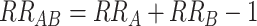; solid line). As described previously, interaction can be assessed by first considering risk among those with both A and B present, next defining a model and scale relating exposure to outcome, and finally comparing observed joint effects with expected joint effects. Consider a scenario where risk among those with neither factor is 1%, factor A increases risk by 1% (i.e., = 0.01, = 2), and factor B increases risk by 1% (i.e., = 0.01, = 2). If observed risk among those jointly exposed to A and B is 4% (i.e.,   = 0.03, = 4), which falls in the dark shaded region between the 2 curves, it is consistent with a superadditive interaction but no interaction on the multiplicative scale. Conversely, an observed risk among those jointly exposed to A and B of 3% corresponds to a submultiplicative interaction but no interaction on the additive scale. If additivity accurately describes the relationship between risk and exposures A and B, then the apparent interaction on the multiplicative scale is strictly a mathematical artifact that results from model misspecification. Table 2 summarizes these scenarios, as well as where direction of interaction depends upon scale (scenario 3).

Figure 1.

Joint effects of A and B (vs. neither) by individual effects. Expected joint effects (i.e., 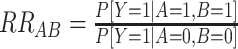) based on individual effects of A (i.e., ) and of B (i.e., 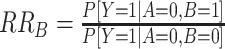) in the absence of interaction when risk is determined multiplicatively (dotted line) or additively (solid line). The unshaded regions correspond to circumstances when conclusions about interaction will be concordant regardless of scale (i.e., supermultiplicative and superadditive or submultiplicative and subadditive). The shaded region indicates circumstances where the 2 scales will yield discordant conclusions. RR, risk ratio.

Table 2.

Scenarios of Risk Related to Exposures A and B and Corresponding Risk Ratios and Risk Differences With Varying Joint Effects Due to the Combination of A and B

Exposure			Jointly		Stratified
A	B	Risk	RR	RD	RR	RD
Scenario 1 a
0	0	0.01	Referent	Referent	Referent	Referent
1	0	0.02	2	0.01	2	0.01
0	1	0.02	2	0.01	Referent	Referent
1	1	0.04	4	0.03	2	0.02
Scenario 2 b
0	0	0.01	Referent	Referent	Referent	Referent
1	0	0.02	2	0.1	2	0.01
0	1	0.02	2	0.01	Referent	Referent
1	1	0.03	3	0.02	1.5	0.01
Scenario 3 c
0	0	0.01	Referent	Referent	Referent	Referent
1	0	0.04	4	0.03	4	0.03
0	1	0.03	3	0.02	Referent	Referent
1	1	0.10	10	0.09	3.3	0.07

Abbreviations: RR, risk ratio; RD, risk difference.

^a For scenario 1, the true scale is additive, and the true joint effect on risk from the combination of A and B is superadditive but with no departure from multiplicativity.

^b For scenario 2, the true scale is additive, and there is no true joint effect on risk from the combination of A and B.

^c For scenario 3, and the true joint effect on risk from the combination of A and B is superadditive (synergistic) but submultiplicative (antagonistic).

CONSIDERATIONS FOR MODELS TO ASSESS INTERACTION

As has been well described, the appropriate scale cannot be determined from data and model fit (8). As a result, when interaction is a central concern for a given epidemiologic study, choice of statistical approach and model scale should match study goals. In order to evaluate whether an exposure has causal effects that depend upon another factor, scale should be consistent with beliefs and current understanding of the true data generating mechanism. Despite the frequent assessment of multiplicative interaction, arguments have been made suggesting additivity as a better representative of models of causality (1, 2, 8), but this remains an open point of debate. In many (most?) instances, evidence regarding the correct scale will be murky. A judicious approach seems merited, whereby interaction on both scales is evaluated. When tests of interaction are concordant across scales, conclusions about presence/absence are simpler, although questions of magnitude will remain unclear. In contrast, when results are discordant, this should be acknowledged. Importantly, if study goals include evaluating potential public health impact of interventions, evaluation of interaction on an additive scale has been advocated regardless of the underlying disease process, because larger subgroup-specific effects on the difference scale identify subgroups that have larger potential for disease prevention (2, 8, 9). Regardless, the approach for assessing interaction should reflect study goals as well as knowledge and uncertainty about links between biological mechanism and statistical model.

REFERENCES

- 1. Rothman KJ. Causes. Am J Epidemiol. 1976;104(6):90–95. [Google Scholar]
- 2. Rothman KJ, Greenland S, Walker AM. Concepts of interaction. Am J Epidemiol. 1980;112(4):467–470. [DOI] [PubMed] [Google Scholar]
- 3. Lawlor DA. Biological interaction: time to drop the term? Epidemiology. 2011;22(2):148–150. [DOI] [PubMed] [Google Scholar]
- 4. Thompson WD. Effect modification and the limits of biological inference from epidemiologic data. J Clin Epidemiol. 1991;44(3):221–232. [DOI] [PubMed] [Google Scholar]
- 5. Walter SD, Holford TR. Additive, multiplicative, and other models for disease risks. Am J Epidemiol. 1978;108(5):341–346. [DOI] [PubMed] [Google Scholar]
- 6. Weinberg CR. Interaction and exposure modification: are we asking the right questions? Am J Epidemiol. 2012;175(7):602–605. [DOI] [PMC free article] [PubMed] [Google Scholar]
- 7. Naimi AI, Whitcomb BW. Estimating risk ratios and risk differences using regression. Am J Epidemiol. 2020;189(6):508–510. [DOI] [PubMed] [Google Scholar]
- 8. Greenland S. Interactions in epidemiology. Epidemiology. 2009;20(1):14–17. [DOI] [PubMed] [Google Scholar]
- 9. VanderWeele TJ, Knol MJ. A tutorial on interaction. Epidemiol Methods. 2014;3(1):33–72. [Google Scholar]