Single‐molecule tracking of Nanog and Oct4 in living mouse embryonic stem cells uncovers a feedback mechanism of pluripotency maintenance

Abstract

Nanog and Oct4 are core transcription factors that form part of a gene regulatory network to regulate hundreds of target genes for pluripotency maintenance in mouse embryonic stem cells (ESCs). To understand their function in the pluripotency maintenance, we visualised and quantified the dynamics of single molecules of Nanog and Oct4 in a mouse ESCs during pluripotency loss. Interestingly, Nanog interacted longer with its target loci upon reduced expression or at the onset of differentiation, suggesting a feedback mechanism to maintain the pluripotent state. The expression level and interaction time of Nanog and Oct4 correlate with their fluctuation and interaction frequency, respectively, which in turn depend on the ESC differentiation status. The DNA viscoelasticity near the Oct4 target locus remained flexible during differentiation, supporting its role either in chromatin opening or a preferred binding to uncondensed chromatin regions. Based on these results, we propose a new negative feedback mechanism for pluripotency maintenance via the DNA condensation state‐dependent interplay of Nanog and Oct4.

Interaction of Nanog and Oct4 with their target DNA loci is prolonged during differentiation to promote pluripotency maintenance.

Introduction

The starting cells for differentiation are embryonic stem cells (ESCs), which can self‐renew and differentiate into most types of cells, termed pluripotency (Beddington & Robertson, 1989). Cell fate determination during differentiation is driven by a dynamic interplay of biological reactions in the nucleus, where the expression of each gene is switched on or off by the binding of transcription factors (TFs) to their target loci, resulting in the patterned expression of regulatory genes. The binding of TFs is regulated by chromatin condensation–relaxation, which is controlled by histone and/or DNA modifications (Lambert et al, 2018; Peñalosa‐Ruiz et al, 2019). Although ESCs are thought to irreversibly lose pluripotency during differentiation into other somatic cells, Takahashi & Yamanaka (2006) demonstrated that pluripotency could be artificially induced or resurrected in somatic cells by exogenously expressing only four specific TFs (Takahashi & Yamanaka, 2006). This experimental fact suggests the cyclic nature of the interplay of the transcription process, epigenetic modification, and chromatin condensation–relaxation. TFs that facilitate effective transcription of their target genes to regulate hundreds of downstream genes for pluripotency induction and maintenance are called core TFs. A working model of how core TFs interact with their target loci in the nucleus for pluripotency maintenance contributes to elucidating the mechanism underlying differentiation and reprogramming and effectively enhances the production and quality control of induced pluripotent stem cells. Many researchers have addressed this issue using various advanced technologies in distinct research fields.

We focused on two core TFs, Nanog and Oct4, which co‐work to stabilise ESCs in the pluripotent state; Nanog buffers the differentiation activity mediated by Oct4 (Loh et al, 2006; Liang et al, 2008). These TFs induce their own expression and mutually activate others, thus resulting in a positive feedback circuit (Pan & Thomson, 2007). For Nanog, by applying molecular expression noise to the feedback circuit, ESCs stochastically fluctuate between two stable states: high and low Nanog expression (Herberg & Roeder, 2015; Marucci, 2017). It has been suggested that the differentiation gate can be opened only when it is in a low‐expression state; hence, Nanog is called a “gatekeeper” (Hyslop et al, 2005). Generally, chromatin condenses during differentiation from an open structure that exposes TF‐binding sites to a closed structure to prevent TF binding (Gaspar‐Maia et al, 2011; Apostolou & Hochedlinger, 2013). Oct4 is responsible for reopening/remodelling closed chromatin and is often called a “pioneer factor” (Soufi et al, 2012; Iwafuchi‐Doi & Zaret, 2014; Xiong et al, 2022). Although the word “pioneer factor” implies “a special factor that actively reopens condensed chromatin,” it was recently proposed that a “pioneer factor” is not a special category of TF but derives from the specific increased affinity of a TF to its locus (Hansen et al, 2022). Numerous studies have supported these hypotheses. In addition, computational experiments interpolate static evidences. Nevertheless, there is still insufficient dynamic observation of functioning proteins on‐site to provide final evidence for these hypotheses and/or propose a new working hypothesis.

Single‐molecule tracking (SMT) based on fluorescence microscopy is the most appropriate tool for investigating the dynamic functions of individual protein molecules of interest on‐site in living cells (Liu & Tjian, 2018; Shao et al, 2018; Lionnet & Wu, 2021). A protein of interest is conjugated with a fluorescent dye one‐to‐one, and even weak fluorescence emitted from a single dye molecule can be detected if the background fluorescence is sufficiently low. However, background fluorescence in conventional fluorescence microscopy conceals a weak fluorescent signal. Total internal reflection fluorescence microscopy (TIRFM) improves the signal‐to‐noise ratio (S/N) to visualise the fluorescence‐coupled protein as a simple fluorescent spot via selective illumination that uses evanescent light generated when the incident light is totally reflected at the interface boundary (Funatsu et al, 1995). TIRFM is limited to observing proteins on or near the plasma membrane attached to a glass surface because the evanescent field is localised on the medium–coverslip interface (Sako & Uyemura, 2002). To observe single molecules inside the nucleus, thinned sheet‐formed light illumination approaches have been developed to achieve a sufficient S/N ratio that detect signals emitted from single dye molecules, although their improvement of the S/N ratio is not as effective as TIRFM (Tokunaga et al, 2008; Gebhardt et al, 2013; Izeddin et al, 2014). Thus, in‐nucleus SMT has been realised to quantitatively investigate the single‐molecule behavioural characteristics of TFs by obtaining kinetic parameters, such as residence time on target loci, fluctuation at the loci, and interaction clustering (Shao et al, 2018).

In SMT, the movements of single molecules are digitally recorded for computer quantification. The distribution of fluorescence emitted from a single individual fluorophore onto the detector surface, called the point spread function (PSF), approximately follows a Gaussian distribution (Thompson et al, 2002). The PSF distribution can be used as a weight to calculate the centre position, intensity, and radial width of the fluorescence distribution. SMT requires the identification and collection of these parameters of as many fluorophores as possible in all acquired images and applies them to appropriate analyses for each object (Liu & Tjian, 2018; Shao et al, 2018; Lionnet & Wu, 2021). Because it is time‐consuming and labour‐intensive to identify each fluorescent spot individually by human eyes, some algorithms that automate this task have been proposed in previous studies, such as SMTracker based on data management via five interactive panels (Rösch et al, 2018), Spot‐ON based on a bias‐corrected modelling framework (Hansen et al, 2018), vbSPT based on a variational Bayesian method of hidden Markov models (Persson et al, 2013), U‐track based on linear assignment problem framework (Jaqaman et al, 2008), dynamic multiple‐target tracing algorithm (Sergé et al, 2008), and multiple threshold methods (Mashanov & Molloy, 2007; Wilson et al, 2016; Yasui et al, 2018). These automatic identifications work well in cases with sufficiently high S/N values. However, in thinned sheet‐formed light illumination, diffusive scattering and refraction due to intracellular microstructure caused by irradiating a cell from the side causes background speckles, which could be misidentified when using low‐intensity dyes, such as genetically encoded fluorescent proteins, or when the intracellular dye concentration is high. In addition, according to the results from a past open competition, there is no SMT algorithm that performs best on all data and in any situation (Chenouard et al, 2014). Therefore, to perform different types of quantitative analysis on the same dataset in the in‐nucleus SMT, optimal parameter tuning is required for each situation, regardless of the method used.

Herein, we performed direct on‐site observation of single molecules of Nanog and Oct4 fused with a fluorescent protein in a living cell nucleus during the loss of pluripotency in mouse ESCs (mESCs) with careful construction of a method of in‐nucleus single‐molecule identification. Quantitative analyses, including residence time on target loci, fluctuation at the loci, and interaction frequency, highlighted the differences between Nanog and Oct4 in single‐molecule dynamics. Remarkably, in common with Nanog and Oct4, interactions of TF with its target loci were found to elongate with DNA fluidity, most likely attributed to chromatin condensation corresponding to the differentiating state, thereby forming a negative feedback loop to maintain their expression. Based on the present results, we propose a new feedback mechanism for pluripotency maintenance using core TFs, Nanog and Oct4. This study demonstrates the veracity of the current hypothesis and provides novel insights into pluripotency maintenance based on single‐molecule quantification.

Results

Single‐molecule observation of Nanog or Oct4 fused with EGFP in mESCs

Endogenous Nanog and Oct4 in mESCs were labelled with a variant of green fluorescent protein derived from Aequorea victoria (Shimomura et al, 1962; Tsien, 1998), enhanced green fluorescent protein (EGFP) (Heim et al, 1995) (Fig 1A). The reasons for selecting EGFP among the GFP variants are described in Supplementary Note S1 and Appendix Figs S1 and S2. The nuclear region of an mESC expressing Nanog‐ or Oct4‐EGFP was selectively illuminated with a sheet‐formed laser using highly inclined and laminated optical sheet microscopy (HILOM) (Tokunaga et al, 2008; Izeddin et al, 2014) (Fig 1B). Nanog‐ or Oct4‐EGFP molecules in the nucleus, indiscriminable under an epi‐fluorescent microscope (Fig 1C, upper panels), were not clearly visualised even under HILOM because the intracellular concentration of EGFP molecules was too high to individually distinguish single molecules. Once all EGFP within the irradiated area in the HILOM was photobleached, only molecules newly entering the irradiated area were discriminably visualised as fluorescent spots (Fig 1C, lower panels and Movie EV1). Because the diffusion of unbound proteins in the nucleus was too fast to be detected during the set exposure time (50 ms), a visible fluorescent spot corresponded to a Nanog‐ or Oct4‐EGFP molecule stably interacting with its target loci on DNA. The duration of the interaction was defined as the time from the appearance to the disappearance of a fluorescent spot on a certain site as a dwell (Fig 1D). Repeated dwell events at a tiny region indicate that Nanog‐ or Oct4‐EGFP molecules interacts with the same locus or other locus within the same tiny region (Fig 1D, yellow lines).

Figure 1. Single‐molecule tracking of Nanog or Oct4 fused with EGFP in mESCs.

1. Cartoon of EGFP‐fused TF (Nanog or Oct4) bound on DNA.
2. Schematic drawing of the present observation with HILOM. To observe a cell at 2–3 μm above the cell surface attached on a glass, the cell was placed slightly lateral to the center of the field of view.
3. Representative image of mESC expressing Nanog‐EGFP in +LIF. Bright field, epifluorescence, HILOM, and a max projection image of 2,000 frames are shown.
4. Typical time course of a Nanog‐EGFP molecule at 450 ms interval in +LIF. Yellow dotted lines indicate the dwell within a 2 μm diameter circular region. White and yellow arrowheads indicate the appearance and disappearance, respectively, of Nanog‐EGFP. The scale bar is 1 μm. It is speculated that the chromatin near the loci where Oct4 is interacting opened when its expression decreased.
5. Histogram of average fluorescent intensity in an mESC expressing Nanog‐EGFP (upper) or Oct4‐EGFP (lower) at various differentiating condition defined as follows: the presence of both LIF and 2i (+2i, red) as the initial condition, 1 day after removing 2i (+LIF, blue), further removal of LIF for 1 day (−LIF, green), and after one another day (−LIF2d, magenta).
6. Confocal images of DRAQ5 staining, showing double‐stranded DNA (top), immunostaining of H3K27ac (middle), and Nanog‐EGFP (bottom), along with the progression of differentiation (+2i, +LIF, −LIF, and −LIF 2d).
7. Swarmplots and violinplots of coefficient of variation of DRAQ5 fluorescence in a nucleus of an mESC expressing Nanog‐EGFP at the condition of +2i (red, n = 20 cells), +LIF (blue, n = 20), −LIF (green, n = 23), −LIF +TSA (light green, n = 22), −LIF2d (purple, n = 21), and −LIF2d +TSA (pink, n = 19). Asterisk and double asterisks indicate P‐value < 0.05 and 0.05 ≤ P‐value < 0.1, respectively, in Student's t‐test.

Leukaemia inhibitory factor (LIF) enhances Nanog and Oct4 expressions, which is necessary to maintain stemness (Matsuda et al, 1999; Hirai et al, 2011). Additionally, MAPK/ERK and GSK3 inhibitors, named 2i, stabilise the pluripotency of mESCs to differentiate into germline cells (Wray et al, 2010). The differentiating conditions were defined by the presence or absence of LIF and/or 2i and the number of days elapsed since the removal of both (see Materials and Methods). The downregulation of Nanog‐ or Oct4‐EGFP expressions due to LIF removal is easily confirmable by observing the decrease in fluorescent cells with fluorescence flow cytometry. However, while the cells in a flow cytometer are unbound, they are bound to the glass surface in the HILOM. Cell adhesion to the substrate affects Nanog and Oct4 expressions in mESCs (David et al, 2019). Therefore, we confirmed the downregulation in our mESC lines under epifluorescent illumination before performing SMT (Fig 1C, upper right). In the presence of both LIF and 2i (+2i), all Nanog‐EGFP‐expressing mESCs exhibited high fluorescence intensity (Fig 1E, upper, red). One day after removing 2i (+LIF), the fluorescence intensity decreased, but EGFP fluorescence remained detectable in almost all mESCs (Fig 1E, upper, blue). Further removal of LIF for 1 day (−LIF) resulted in fluorescence loss in some mESCs (Fig 1E, upper, green, arrowhead). Then, after another day (−LIF2d), the cells turned non‐fluorescent or too dark to be detected (Fig 1E, upper, magenta). In the case of Oct4‐EGFP‐expressing mESCs, fluorescence was maintained until the first day after removing LIF and was almost lost by the second day (Fig 1E, lower).

Next, we confirmed the chromatin condensation and acetylation of histone H3 at lysine 27 (H3K27ac), which depended on the differentiation conditions, using confocal fluorescence microscopy (Fig 1F). Bright foci were interspersed in a DNA staining image (Fig 1F, top), the fluorescence signal decreased in a H3K27ac immunostaining image (Fig 1F, middle), and Nanog‐EGFP‐negative mESCs were present (Fig 1F, bottom), all depending on the differentiation conditions. Chromatin condensation could be roughly quantified by calculating the coefficient of variation (C.V.), which is the ratio of standard deviation and average intensity, of DRAQ5 fluorescence in the nucleus, which indicates the spatial heterogeneity of the stained DNA (Fig 1G). The C.V. significantly increased after the removal of 2i (Fig 1G, red and blue; P = 2.4 × 10⁻⁵ in Student's t‐test), but was not further increased by the subsequent LIF removal (Fig 1G, green; P = 0.33 in Student's t‐test), demonstrating that there was no obvious difference in chromatin condensation status in the multicellular average before and after the LIF removal. Two days after the removal of 2i and LIF, more cells exhibited an even higher C.V. and wider population distribution (Fig 1G, purple). The addition of 0.5 μM Trichostatin A (TSA), a well‐known histone deacetylase inhibitor used as a chromatin decondensation agent, in culture medium caused a decrease in C.V., indicating the effectiveness of TSA treatment (Fig 1G, light green and pink). Notably, EGFP molecules were not detected in EGFP‐negative mESCs, even when HILOM was used (Fig 1F, −LIF, right). Inevitably, we selectively observed Nanog‐ or Oct4‐EGFP expressing mESCs (Fig 1F, −LIF, left). Thus, we observed mESCs only immediately before the loss of pluripotency.

Optimization of autoidentification protocol of single molecules

Various automation algorithms for single‐molecule identification and tracking have been developed (Jaqaman et al, 2008; Sergé et al, 2008; Persson et al, 2013; Hansen et al, 2018; Rösch et al, 2018). We employed a multiple threshold method (Mashanov & Molloy, 2007; Wilson et al, 2016; Yasui et al, 2018), which is the simplest and most intuitive method for biologists, and performed the following parameter optimisation.

To estimate the centre position (x ₀ [pixels], y ₀ [pixels]), intensity (I [a.u.]), and radial width (σ [pixels]) of a single fluorescent spot, a method was selected based on Gaussian fitting (Thompson et al, 2002; Ichimura et al, 2014), in which the parameters were obtained by fitting an image of a single fluorophore within a circle‐formed region of interest (ROI) of nine pixels in diameter. This selection was made because Gaussian fitting has the highest robustness at low S/N data compared to other methods, such as cross‐correlation, sum‐absolute difference, or simple centroid calculation (Thompson et al, 2002). Additionally, we assumed a tilted planar background in a limited area within the ROI in the Gaussian fitting approximation (Fig 2A and see Materials and Methods) (Ichimura et al, 2014). As truly identified molecules, we collected data on 8,645 single fluorescent spots that were individually identified by the human eye (hereinafter, “manual picking”) (Fig 2B, black). Here, the ROI where the iterative Gaussian fitting converged was comprehensively stored by scanning within the nucleus region in a collection. The I–σ correlation plot of all calculated solutions exhibited a wider distribution than that of manual picking (Fig 2B, green), indicating that the solution for Gaussian fitting might converge even if no fluorescent molecule exists. Therefore, the threshold I (Th _(I) [a. u.]) and/or threshold σ (Th _(σ) [pixels]) are generally used to distinguish between ROIs with and without a fluorescent spot (Fig 2B and C, broken red lines) (Yasui et al, 2018).

Figure 2. Optimisation of auto‐identification protocol of single individual molecules.

1. Typical cross‐section of a fluorescent spot of Nanog‐EGFP in an mESC and explanation of the fitting parameters. The red line is the fitting result with a Gaussian function with assuming the planar background (BG). The inset is a fluorescent image of single Nanog‐EGFP molecule. Diameter of a circle ROI was 9 pixels (yellow broken line).
2. I–σ plot of the results of Gaussian fitting for Nanog‐EGFPs in a nucleus by manual picking (black), those by the automated identification (green), and those screened with thresholds of Th _(C) = 5 (orange) and Th _(C) = 7 (blue).
3. Five typical examples of time courses of I in a trajectory of true single molecules.
4. Three typical examples of time course of I in a trajectory including false positives. Insets in (C and D) are the time course of the ROI (cyan circle) in which I was estimated. Values in (C and D) indicate the average value of I in a trajectory, I _ave. Red broken lines indicate I = 250. Asterisks indicate blinking points when Th _(I) = 250.
5. Histograms of I _ave of the result screened with thresholds of Th _(I) = 0, Th _(σ) = 0, Th _(R) = 1, and Th _(C) = 3 (green), Th _(C) = 5 (orange), or Th _(C) = 7 (blue). The one obtained by manual picking was superimposed in grey. Magenta is one with thresholds of Th _(I) = 250, Th _(σ) = 1.0, Th _(R) = 1, and Th _(C) = 5.
6. Cumulative histogram of dwell time obtained with 50 ms interval (upper) and MSD plot (lower) using single‐molecule data of Nanog‐EGFP screened by manual tracking (grey) and with thresholds of Th _(R) = 1, Th _(C) = 5, Th _(I) = 250, and Th _(σ) = 1 (magenta) or Th _(R) = 1, Th _(C) = 7, Th _(I) = 0 and Th _(σ) = 0 (blue), and the present protocol (red).
7. Histograms of I of the result screened by the present protocol: green, the first screening with Th _(C) = 3 and Th _(R) = 1; blue, the second screening with Th _(Iave) = 600; red, the final screening with Th _(C) = 5 and Th _(R) = 2. That obtained by manual picking was superimposed in grey.

Because TFs bind and remain in a locus, trajectories of time development after a spot appear within a limited range (Th _(R) [pixels]) could be extracted using the threshold for the continuity of the fluorophore (Th _(C) [frames]) (Fig 2C and D), resulting in screening out misidentification, even without thresholds using Th _(I) or Th _(σ) (Fig 2B, orange and blue) (Mashanov & Molloy, 2007; Wilson et al, 2016). Th _(R) and Th _(C) also played a role in refusing spots exhibiting rapid diffusion of unbound TF, similar to a method of selectively detecting only slow diffusion molecules by enhancing the motion blurring effect with a long exposure time in image acquisition (Etheridge et al, 2014). However, the collected trajectories with the thresholds of Th _(R) and Th _(C) included false positives owing to the small sequential speckles (Fig 2D, upper) or a combination of these and the one‐frame appearance of a fluorophore (Fig 2D, lower). False positives were reflected in the histogram of the average I‐values within a trajectory (I _ave) (Fig 2E). When Th _(C) = 3, a lower I‐value population was observed compared to that of manual picking (Fig 2E, green). When Th _(C) was increased to 5, the low I‐value population decreased but still remained (Fig 2E, orange). The additional use of Th _(I) and Th _(σ) or further increase in Th _(C) to 7 showed approximately the same distribution as the manual tracking data (Fig 2E, magenta and blue), indicating the effective removal of false positives.

Furthermore, test analyses of dwell time and mean square displacement (MSD) were conducted using the data screened with thresholds showing fewer failures on the I _ave histogram. Because the fluorescence of the dye was zero in the blinking events, the allowance of one dark frame within a continuous spot could prevent tracking from an interruption in the middle (Fig 2C, asterisks), as previously reported (Gebhardt et al, 2013). The dwell time histograms and the MSD plot of the screened fluorescent spots differed from those made of 302 traces tracked by the human eye (hereinafter, “manual tracking”), and the dwell time and MSD values were underestimated (Fig 2F). More details are provided in Supplementary Note S2 and Appendix Figs S3–S6.

Hence, we developed a three‐step screening method by applying an additional threshold, I _ave (Th _(Iave) [a.u.]). First, all ROIs where the iterative solution converged were screened with Th _(I) = 250, Th _(σ) = 1, Th _(R) = 1, and Th _(C) = 3. Some false positives remained after the first step, as shown in the histogram of I (Fig 2G, green). Second, Th _(Iave) was set to 600 to exclude 99% of the false positives while missing 10% of the short dwell trajectories. The shape of histogram I was almost the same as that obtained by manual picking (Fig 2G, blue), indicating that the overall population included almost all correct single molecules after screening with Th _(Iave). Finally, the remaining spots were rescreened with thresholds of Th _(R) = 2 and Th _(C) = 5 to conjugate the short‐trajectory fragments. In the final step, up to four consecutive dark frames in an existing continuous trajectory were allowed, whereas only one frame was allowed in the first step. The shape of histogram I did not change between before and after the final step (Fig 2G, red), indicating no further failures. The dwell time histograms and MSD plot of Nanog‐EGFP in the nucleus using this protocol were almost the same as those of manual picking (Fig 2F, red). Considering that the illumination intensity in the HILOM varied for each cell, unlike the TIRFM, we additionally developed a method to adaptively set Th _(I) and Th _(Iave) for each cell. Thus, we established an automated protocol to obtain the same results as manual picking/tracking. More details are provided in Supplementary Note S3 and Appendix Figs S7–S9.

Analysis of dissociation rate of Nanog or Oct4‐EGFP on its target loci

First, we analysed the dissociation rate, which is the reciprocal of the interaction time, of Nanog‐ or Oct4‐EGFP from their target loci, and investigated the dependence of this rate on differentiation conditions. The time courses of parameter I on a fixed ROI clearly showed the appearance and disappearance of a fluorescent spot (Fig 3A). While the appearance corresponded to the binding events of Nanog‐ or Oct4‐EGFP (Fig 3A, green arrows), the disappearance included alternative possibilities of dissociation and photobleaching (Fig 3A, red arrows). Because the photobleaching rate of EGFP when fixed on glass surface was 0.077 ± 0.010 frame⁻¹ (N = 4,772 molecules) in our microscope condition, the dissociation rate of Nanog‐ or Oct4‐EGFP was expected to be lower than the photobleaching rate of fluorescent proteins in SMT at frame periods below 600 ms, considering the dissociation rate of other TFs (0.10–0.12 s⁻¹) previously reported (Xie et al, 2017). Meanwhile, using longer intervals, the entire cell movement possibly causes interruption of tracking. A method to solve this problem was previously developed because the dissociation rate is independent of the frame period and photobleaching is dependent; these can be mathematically distinguished by collecting the dwell time data at various frame periods (Gebhardt et al, 2013). The dwell events were distributed throughout the nucleus regardless of the different (50, 100, 150, 250, and 450 ms) frame periods (Fig 3B; Supplementary Note S4 and Appendix Fig S10). We estimated the frame period independent term, i.e., the dissociation rate k _off , of Nanog‐ and Oct4‐EGFP in an mESC using a modified version of the previous method. The k _off was calculated for each cell by globally fitting its dwell time histogram for all frame periods with an equation assuming two photobleaching processes and one dissociation process (Fig 3C; Supplementary Note S4 and Appendix Figs S11–S13; see Materials and Methods). The dwell time histograms, including all cell data, highlighted the overall differences in k _off among the conditions of +2i, +LIF, and −LIF for both Nanog‐ and Oct4‐EGFP (Fig 3D).

Figure 3. Analysis of dissociation rate of Nanog‐ or Oct4‐EGFP on its target loci.

1. Typical three time‐courses of parameter I, the fluorescent intensity of a single fluorophore, on a fixed ROI. Asterisks indicate blinking events of the fluorescent protein. Arrows indicate events of appearance and disappearance of the fluorescent spots.
2. Typical example of all dwell trajectories of Nanog‐EGFP obtained within every 400 frames at frame periods of 50 (green), 100 (orange), 150 (red), 250 (magenta), and 450 ms (blue) in a nucleus in +LIF.
3. Typical example of dwell time histograms of Nanog‐EGFP obtained within every 400 frames at frame periods of 50 (green, n = 228 traces), 100 (orange, n = 97), 150 (red, n = 102), 250 (magenta, n = 124), and 450 ms (blue, n = 157) in a nucleus in +LIF.
4. Dwell time histograms of Nanog‐EGFP (left) and Oct4‐EGFP (right) obtained from all cell data (n = 73 in +2i, 65 in +LIF, and 66 cells in −LIF for Nanog‐EGFP, and n = 57 in +2i, 53 in +LIF, and 58 cells in −LIF for Oct4‐EGFP) at frame periods of 50, 100, 150, 250, and 450 ms in a nucleus in +2i (red), +LIF (blue), and −LIF conditions (green). Values of k _off were obtained by the global fitting approximation.
5. Histograms of dissociation rate of Nanog‐EGFP (left) and Oct4‐EGFP (right) in an mESC in +2i (top), +LIF (middle), and −LIF (bottom) conditions. Black line shows the fitting result with a normal distribution.
6. Dependence of expression level of Nanog‐EGFP (upper) and Oct4‐EGFP (lower) on dissociation rate. Considering the distribution of the fluorescent intensity (Fig 1E), low (blue), middle (magenta), and high (red) were defined as cells showing the log value of the fluorescent intensity of < 1.9, 2.0–2.3, and > 2.4 [a.u.], respectively, for Nanog‐EGFP or < 1.9, 2.0–2.2, and < 2.3 [a.u.], respectively, for Oct4‐EGFP. Bars and error bars are mean ± SD. For Nanog‐EGFP, N = 20 (high), 32 (middle) and 20 (low) for +2i, 26 (high), 18 (middle) and 21 (low) for +LIF, and 20 (high), 26 (middle) and 20 cells (low) for −LIF. For Oct4‐EGFP, N = 22 (high), 18 (middle) and 17 (low) for +2i, 17 (high) 16 (middle) and 20 (low) for +LIF, and 19 (high), 19 (middle) and 20 cells (low) for −LIF. Asterisks indicate less than 0.05 of the P‐value in Student's t‐test.

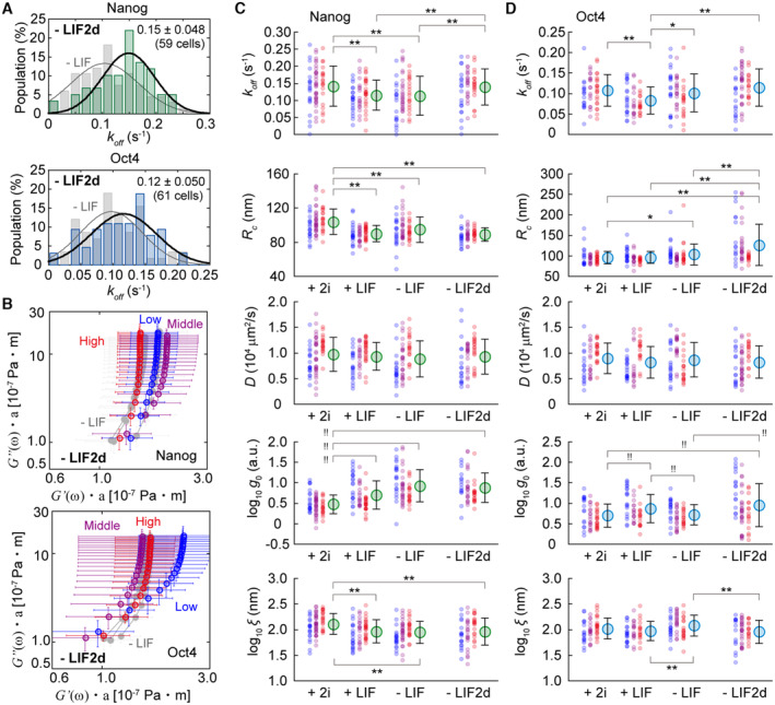
The k _off of Nanog‐ and Oct4‐EGFP in an mESC exhibited different behavioural characteristics under +2i, +LIF, and −LIF conditions (Fig 3E and F). The mean k _off of Nanog‐EGFP in +2i was 0.14 s⁻¹, which significantly decreased to 0.11 s⁻¹ in +LIF (P = 0.0031 in Student's t‐test), and further decreased but insignificantly to 0.10 s⁻¹ in −LIF (P = 0.80 in Student's t‐test) (Fig 3E, left). Meanwhile, k _off of Oct4‐EGFP decreased after the 2i removal from 0.11 s⁻¹ to 0.08 s⁻¹ (P = 3.6 × 10⁻⁴ in Student's t‐test), and then returned to 0.10 s⁻¹ after the LIF removal (P = 0.013 in Student's t‐test) (Fig 3E, right). Based on the classification into three categories depending on its expression level (low, middle, and high; see the legend of Fig 3F), the mean k _off positively correlated with the expression level in Nanog‐EGFP, although statistically insignificant, except for that in the low expression in –LIF (Fig 3F, upper). In Oct4‐EGFP, almost no significant difference was observed between the expression levels under the 2i condition, and k _off was negatively correlated in +LIF and −LIF (Fig 3F, lower). Thus, Nanog‐EGFP appeared to interact longer with its target loci when differentiating and/or decreasing its expression level, whereas Oct4‐EGFP showed the opposite response at decreased expression levels.

Analysis of fluctuating movements of Nanog‐ or Oct4‐EGFP on its target loci

Chromatin condensation corresponding to the differentiation state alters the physical properties of DNA, which is reflected in the fluctuating movements of Nanog‐ or Oct4‐EGFP binding on the DNA. Next, the relationship between the differentiation state or expression level and the physical properties of the binding site was investigated using MSD analysis, thereby enabling the quantification of fluctuating movements (Fig 4A) (Kusumi et al, 1993; Saxton & Jacobson, 1997; Martin et al, 2002; Liu & Tjian, 2018). Because the average MSD curve appeared saturated (Fig 4B), two parameters, namely confined radius (R _c ) and diffusion coefficient (D), could be estimated (Kusumi et al, 1993; Miné‐Hattab & Xavier, 2020). R _c and D are thought to reflect chromatin condensation and local viscoelasticity, respectively, near the target loci of TFs (Lerner et al, 2020; Miné‐Hattab & Xavier, 2020; Lionnet & Wu, 2021).

Figure 4. Analysis of fluctuating movements of Nanog or Oct4‐EGFP on its target loci.

• A
  Cartoon of the fluctuating movement of EGFP molecules on a DNA chain and three typical trajectories of Nanog‐EGFP.
• B
  A typical example of an MSD plot of Nanog‐EGFP in an mESC in +2i. The orange lines indicate each MSD curve obtained from a trajectory of an individual molecule. The red plots are the averages of the 1,459 single MSD curves within a cell. Error bars represent the standard deviation.
• C
  Histograms of R _c of Nanog‐EGFP (left) and Oct4‐EGFP (right) in an mESC in +2i (top), +LIF (middle), and −LIF (bottom). The black line shows the fitting result with a normal distribution.
• D, E
  Dependence of expression level of Nanog‐EGFP (left) and Oct4‐EGFP (right) on R _c (D) or D (E). Bars and error bars are mean ± SD. For Nanog‐EGFP, N = 20 (high), 32 (middle) and 20 (low) for +2i, 26 (high), 18 (middle) and 21 (low) for +LIF, and 20 (high), 26 (middle) and 20 cells (low) for −LIF. Of Oct4‐EGFP, N = 22 (high), 18 (middle) and 17 (low) for +2i, 17 (high) 16 (middle) and 20 (low) for +LIF, and 19 (high), 19 (middle), and 20 cells (low) for −LIF. Asterisks and double asterisks indicate P‐values of less than 0.05 and 0.01, respectively, in Student's t‐test.
• F
  A typical example of microrheology analysis of Nanog‐EGFP in an mESC in +2i. Laplace transformation was applied to an average MSD shown in (B).
• G, H
  G″(ω)–G′(ω) plot of Nanog‐EGFP (G) and Oct4‐EGFP (H) categorised with expression level. Error bars represent standard deviations. For Nanog‐EGFP, N = 20 (high), 32 (middle) and 20 (low) for +2i, 25 (high), 18 (middle) and 20 (low) for +LIF, and 20 (high), 26 (middle) and 19 cells (low) for −LIF. For Oct4‐EGFP, N = 21 (high), 18 (middle) and 17 (low) for +2i, 22 (high) 19 (middle) and 20 (low) for +LIF, and 18 (high), 19 (middle), and 20 cells (low) for −LIF.

Data information: The definition of low (blue), middle (magenta), and high (red) in (D, E, G, and H) were the same as that of Fig 3F.

The R _c of Nanog‐EGFP significantly decreased after the removal of 2i (P = 1.4 × 10⁻⁹ in Student's t‐test), but did not further decrease after further removing LIF (P = 0.026 in Student's t‐test) (Fig 4C, left), suggesting that chromatin condensation near Nanog's target loci had already begun when removing 2i, which was consistent with the results of nuclear staining (Fig 1F, top panels and Fig 1G). Oct4‐EGFP did not exhibit significant differences among the three conditions (Fig 4C, right). In terms of expression dependence, the R _c in +2i positively correlated with the Nanog‐EGFP expression level, whereas those in +LIF and −LIF did not (Fig 4D, left). The R _c of Oct4‐EGFP under all conditions tended to negatively correlate with the expression level (Fig 4D, right), indicating that the DNA near the loci to which Oct4 interacted was a flexible structure when mESCs expressed less Oct4. This tendency was similar to that of the k _off analysis (Fig 3F, lower), implying a relationship between the dissociation rate and chromatin condensation. Meanwhile, there was no significant difference between D among the different conditions in either Nanog‐ and Oct4‐EGFP, and it was negatively correlated with the expression level in both Nanog‐ and Oct4‐EGFP, except for the −LIF condition in Oct4‐EGFP (Fig 4E).

To further consider viscoelasticity, we separately calculated the dynamic moduli of elasticity and viscosity, storage shear modulus (G′(ω)), and loss shear modulus (G″(ω)) (see Materials and Methods) because the generalised Stokes–Einstein relationship connects the MSD to the complex shear moduli in the Laplace domain (Ferry, 1980; Shinkai et al, 2020a, 2020b). G″(ω) was linearly correlated with frequency (ω) in all cases (Fig 4F, left). The ratio of G″(ω) to G′(ω) was almost > 1.0 in all cases, indicating a liquid‐like feature rather than a solid‐like feature (Fig 4F, right). The G′(ω) of Nanog‐EGFP matched the general expectation based on chromatin condensation: higher expression or less differentiation, lower G′(ω); lower expression or more differentiation, higher G′(ω) (Fig 4G). Generally, when G′(ω) and G″(ω) are proportional to ω ² and ω, respectively, the system relaxes to achieve the slowest molecular motion. While only G″(ω) was proportional to ω, which indicates relaxed fluidic behaviour, the elastic component behaviour of G′(ω) deviated from this trend. Furthermore, comparisons with the differentiation state and expression level highlighted a change in G′(ω). Oct4‐EGFP showed an interesting behaviour. While the tendency was almost the same as that of Nanog‐EGFP in +2i (Fig 4H, top), lower expression decreased G′(ω), lowering the elasticity in +LIF (Fig 4H, middle). The removal of LIF eliminated the dependence on expression level in the G″(ω)–G′(ω) plot of Oct4‐EGFP (Fig 4H, bottom). Thus, there was a clear difference in DNA viscoelasticity near the TF locus between Nanog‐EGFP and Oct4‐EGFP during mESC differentiation.

Analysis of repeated interaction of Nanog or Oct4‐EGFP on its target loci

Visualising the dwelling frequency per unit area in colour highlighted some sites in which the probability of dwell events was increased by removing 2i (Fig 5A). TFs have been reported to have different affinities for each locus and preferentially bind to high‐affinity loci, corresponding to the cellular states (called hotspots) observed under HILOM (Kitagawa et al, 2017). We quantified the frequency of the dwell events of Nanog‐ or Oct4‐EGFP during differentiation using pair correlation analysis (Sengupta & Lippincott‐Schwartz, 2012; Sengupta et al, 2013). The pair correlation function g(r) is the probability that another particle exists on the circumference of radius r and width δr centred on a given particle, normalised by the particle density (Fig 5B, left). g(r) is usually approximated with a single exponential curve, where the intercept (g ₀) and the exponential decay constant (ξ) express the mean particle existence probability and the mean cluster size at a given clustering site, respectively (Sengupta & Lippincott‐Schwartz, 2012). Here, a particle corresponds to the average centre position of a spot moving during a dwell event, and particle clustering corresponds to repeated interactions with the same dwell site. Briefly, g ₀ and ξ reflects the mean occurrence probability of the dwell event and slow positional mobility derived from the fluidity of the DNA chain near a locus, respectively (Fig 5B, right).

Figure 5. Analysis of repeated interactions of Nanog‐ or Oct4‐EGFP on its target loci.

• A
  Visualisation of the dwelling frequency of Nanog‐EGFP per unit area, referred to as density, in an mESC in +2i (left) and +LIF (right). The colour corresponds to the density of Nanog dwell events (events/μm²) within 2,000 frames.
• B
  Explanatory drawing of the pair correlation analysis. The calculation of the probability of Nanog‐ or Oct4‐EGFP molecule dwelling to another site at a given distance from a dwelling site provides the comparison to randomly dwelling.
• C, D
  The average correlation index g(r) of Nanog‐EGFP (C) and Oct4‐EGFP (D) in +2i (top), +LIF (middle), and −LIF (bottom). Insets are histograms of logarithm value of the intercept g ₀ (magenta) and the exponential decay constant ξ (orange) of single mESCs. Black lines in insets show the fitting results with a normal distribution. Error bars represent the standard deviation. N = 72 for +2i, 56 for +LIF and 56 cells for −LIF of Nanog‐EGFP, and N = 57 for +2i, 53 for +LIF and 58 cells for −LIF of Oct4‐EGFP.
• E, F
  Dependence of expression level of Nanog‐EGFP (left) and Oct4‐EGFP (right) on log₁₀ g ₀ (E) and log₁₀ ξ (F). Error bars represent standard deviations. The definition of low (blue), middle (magenta), and high (red) in E and F were the same as that of Fig 3F. Bars and error bars are mean ± SD. Of Nanog‐EGFP, N = 20 (high), 32 (middle) and 20 (low) for +2i, 26 (high), 18 (middle) and 21 (low) for +LIF, and 20 (high), 26 (middle) and 20 cells (low) for −LIF. Of Oct4‐EGFP, N = 22 (high), 18 (middle) and 17 (low) for +2i, 17 (high) 16 (middle) and 20 (low) for +LIF, and 19 (high), 19 (middle) and 20 cells (low) for −LIF. Asterisks and double asterisks indicate P‐values of less than 0.05 and 0.01, respectively, in Student's t‐test. Exclamation marks and double exclamation marks indicate P‐values of less than 0.05 and 0.01, respectively, in Mann–Whitney's U‐test.

The average trace of g(r) showed an increase in the average g ₀ and a decrease in the average ξ as differentiation progressed for Nanog‐EGFP (Fig 5C). In contrast, the average g ₀ of Oct4‐EGFP increased with the removal of 2i, as did Nanog‐EGFP, and recovered with the removal of LIF, while there was no clear difference in the average ξ (Fig 5D). While the average g ₀ of Nanog‐EGFP increased after removing 2i and further increased on average after removing LIF (Fig 5C), the histograms of the log₁₀ g ₀ for Nanog‐EGFP highlighted the appearance of the second population with large values with the removal of 2i, and the mean values of the two populations increased with the removal of LIF (Fig 5C, insets, left). Two populations were also observed for Oct4‐EGFP, even in the presence of 2i, and the mean value of the second population increased with the removal of 2i and markedly decreased with the removal of LIF (Fig 5D, insets, left). The log₁₀ ξ for Nanog‐EGFP decreased without any change in the distribution feature by removing 2i, but not LIF (Fig 5C, inset, right). The log₁₀ ξ for Oct4‐EGFP did not change after removing 2i (P = 0.18 in Student's t‐test) but was significantly increased by removing LIF (P = 3.2 × 10⁻³ in Student's t‐test) (Fig 5D, insets, right). The expression dependence of log₁₀ g ₀ exhibited a negative correlation under all conditions for both Nanog‐ and Oct4‐EGFP (Fig 5E). Meanwhile, those of log₁₀ ξ exhibited a positive correlation in almost all cases, except for the −LIF condition of Oct4‐EGFP (Fig 5F).

Assuming that chromatin condensation and the increase in repeated interactions corresponded to the differentiation stage and that the R _c and g ₀ for Nanog‐ and Oct4‐EGFP reflected them, the changing moment of R _c and g ₀ should be captured during the cell state transition. As expected, by observing the time development of Nanog‐EGFP under −LIF conditions, we obtained data showing that R _c and g ₀ dynamically increased at any time within 100 min after LIF removal (Fig 6A and B). Using such data, the emergence of hotspots of functioning Nanog could also be visualised (Fig 6C).

Figure 6. Analysis of dynamic change of repeated interactions of Nanog‐EGFP in a living mESC.

• A
  Average time development of R _c of Nanog‐EGFP in the presence of 2i and LIF (red) and 6 h after removing the both (green). Error bars represent standard deviations. N = 6 cells for +2i and 13 cells for −LIF, respectively.
• B, C
  A typical example of time developments of correlation index g(r) (B) and visualisation of the binding frequency of Nanog‐EGFP per unit area (density) (C) in a mESC 6 h after the removal of 2i and LIF. Colour in (C) corresponds to the density of Nanog dwell events (events/μm²) within 2,000 frames. These were obtained from the same cell. Arrows indicate the emergence of hotspots of functioning Nanog, exhibiting obviously higher density than the others.

Change in parameters two days after removal of 2i and LIF

Two days after removing 2i and LIF (−LIF2d), the expression levels of both Nanog‐ and Oct4‐EGFP decreased, making it difficult to compare the single‐molecule data at the same expression level before the −LIF condition (Fig 1E, purple). Nevertheless, considering the importance of the data obtained in differentiated mESCs, we collected data of mESCs with residual fluorescence in the −LIF2d condition and performed the same analyses. The k _off of Nanog‐EGFP returned to the similar value as that in +2i (Fig 7A, upper), whereas that of Oct4‐EGFP exhibited a slight but insignificant increase (Fig 7A, lower). The viscoelasticity obtained using microrheology analysis showed no obvious change in Nanog‐EGFP (Fig 7B, upper). In Oct4‐EGFP, G′(ω) remarkably increased in the case of low expression, indicating that the DNA was transferred more elastically (Fig 7B, lower).

Figure 7. Data obtained two days after removal of 2i and LIF and summary of all data.

• A
  Histograms of the dissociation rate of Nanog‐EGFP (upper) and Oct4‐EGFP (lower) in an mESC in the condition of −LIF2d. The black line shows the fitting result with a normal distribution.
• B
  G″(ω)–G′(ω) plot of Nanog‐EGFP (upper) and Oct4‐EGFP (lower) categorised with expression level. In −LIF2d, the low (blue), middle (magenta), and high (red) were defined as cells showing the log value of the fluorescent intensity of < 1.7, 1.8–2.1, and > 2.2 [a.u.], respectively, for Nanog‐EGFP or < 1.5, 1.6–1.9, and > 2.0, respectively, for Oct4‐EGFP. Error bars represent standard deviations. For Nanog‐EGFP, N = 20 (high), 19 (middle) and 17 (low) for −LIF2d. Of Oct4‐EGFP, N = 17 (high), 19 (middle) and 13 (low) for −LIF2d.
• C, D
  Plots of all data of cells categorised with expression level (red, magenta, and blue) and with the mean values (green or cyan) in each parameter in each condition of Nanog‐EGFP (C) or Oct4‐EGFP (D). The definition of low (blue), middle (magenta), and high (red) in +2i, +LIF, and −LIF were the same as that of Fig 3F, and those in −LIF2d were the same as (B) in this figure. Error bars represent standard deviations. For Nanog‐EGFP, N = 20 (high), 32 (middle) and 20 (low) for +2i, 26 (high), 18 (middle) and 21 (low) for +LIF, 20 (high), 26 (middle) and 20 cells (low) for −LIF, and 20 (high), 20 (middle) and 19 cells (low) for −LIF2d. For Oct4‐EGFP, N = 22 (high), 18 (middle) and 17 (low) for +2i, 17 (high) 16 (middle) and 20 (low) for +LIF, 19 (high), 19 (middle) and 20 cells (low) for −LIF, and 16 (high), 29 (middle) and 16 cells (low) for −LIF2d. Asterisks and double asterisks indicate P‐values of less than 0.05 and 0.01, respectively, in Student's t‐test. Exclamation marks and double exclamation marks indicate P‐values of less than 0.05 and 0.01, respectively, in Mann–Whitney's U‐test. Note: the data obtained in −LIF2d could not simply compare with the others because the expression levels differed between them.

We listed 10 graphs of each parameter for all obtained data to explore the overall tendency (Fig 7C and D). In Nanog‐EGFP‐expressing mESCs, the dependence of the obtained parameters on the differentiating conditions correlated with each other until a day after the removal of 2i and LIF (Fig 7C). The additional day did not alter R _c , D, g ₀, or ξ, but did alter k _off (Fig 7C, −LIF2d). The dependence on the expression level showed the same trend under all conditions and parameters (Fig 7C; red, blue, and magenta). However, k _off and D did not depend on the differentiation conditions of Oct4‐EGFP‐expressing mESCs (Fig 7D, top and middle). The R _c in Oct4‐EGFP increased with an additional day, particularly in the middle and low expression levels (Fig 7D, second top), and g ₀ and ξ returned to the same value as that in +LIF (Fig 7D, second bottom and bottom). The dependencies on the expression level also returned to those observed in +LIF (Fig 7C, red, blue, and magenta). Notably, eliminating the data obtained in the +2i condition based on the assumption that the 2i addition induced a peculiar stable state in mESCs, differentiation can be defined as progressing with time just after LIF removal. Under this definition of differentiation, k _off on average can be interpreted as increasing with differentiation progression for both Nanog and Oct4 (Fig 7C, upper).

Correlation between k _off and the other parameters

Finally, the correlations between the obtained parameters were investigated. While the log₁₀ g ₀₋ k _off correlation depended on the culture conditions for both Nanog‐EGFP and Oct4‐EGFP, the dependence differed between Nanog‐EGFP and Oct4‐EGFP (Fig 8A, left and centre). Meanwhile, the log₁₀ ξ–k _off correlation was interdependently distributed with the same linear relationship, regardless of the culture conditions for Oct4‐EGFP (Fig 8A, right). Even though log₁₀ g ₀ and log₁₀ ξ were negatively correlated, for example, (Pearson correlation coefficient) = −0.77 in +2i, = −0.76 in +LIF, and = −0.65 in −LIF for Oct4‐EGFP, the correlation between log₁₀ g ₀ or log₁₀ ξ and k _off was different (Fig 8A, centre and right), implying that k _off was independently and respectively related to log₁₀ g ₀ and log₁₀ ξ. Heatmaps of the Pearson correlation coefficient of k _off and each parameter highlighted the differences between Nanog‐EGFP and Oct4‐EGFP (Fig 8B). For Nanog‐EGFP, k _off was generally positively or negatively correlated with any parameter, and the correlations were relatively weak under the +2i condition and tended to be stronger after LIF removal (Fig 8B, upper). Oct4‐EGFP exhibited a complicated behaviour in the correlations: the correlation with expression level turned from positive to negative in +LIF and −LIF condition (Fig 8B, lower); the positive correlation with D was observed only in −LIF condition; oppositely, the correlation with log₁₀ g ₀ was not observed only in −LIF condition; and the log₁₀ ξ for Oct4‐EGFP stably correlated independent of the culture condition.

Figure 8. Correlation analyses of the obtained parameters.

1. Correlation plots of log₁₀ g ₀ and k _off of Nanog‐EGFP (left) and Oct4‐EGFP (centre) and log₁₀ ξ and k _off of Oct4‐EGFP (right) in 2i (top), +LIF (middle) and −LIF (bottom) conditions. Each plot indicates the average value in a single cell. Lines are fitting results with a liner function.
2. Heatmaps of the Pearson correlation coefficient of k _off and each parameter in 2i, +LIF, −LIF, and −LIF2d conditions. Numbers indicate the respective Pearson correlation constants, coloured from −0.5 (blue) to 0.5 (red).
3. Network graphs whose nodes connected with Pearson correlations of each parameter pair of Nanog‐EGFP (upper) and Oct4‐EGFP (lower) in 2i, +LIF, −LIF, and –LIF 2d conditions. The sign and the strength of each correlation from −0.5 to 0.5 in terms of transparency from 0 to 100% of the connecting lines. The colour of the connecting line is the same as that described in (B).
4. Effect of 0.5 μM TSA addition on log₁₀ g ₀ of Nanog‐EGFP (left) and Oct4‐EGFP (right) in +LIF (filled) and –LIF (opened). Error bars represent standard deviations. For Nanog‐EGFP, N = 65 for +LIF –TSA, 91 for +LIF +TSA, 66 for –LIF –TSA, and 88 cells for –LIF +TSA. For Oct4‐EGFP, N = 53 for +LIF –TSA, 42 for +LIF +TSA, 58 for –LIF –TSA, and 39 cells for –LIF +TSA. Exclamation marks and double exclamation marks indicate P‐values of less than 0.05 and 0.01, respectively, in Mann–Whitney's U‐test.
5. Network graphs whose nodes connected with Pearson correlations of each parameter pair of Nanog‐EGFP (upper) and Oct4‐EGFP (lower) in 2i, +LIF, –LIF, and –LIF 2d conditions in the presence of 0.5 μM TSA. The colour and the transparency of the connecting line are the same as that described in (B).

To exhibit the correlation between parameters more visually, network graphs were displayed showing the sign and strength of each correlation in terms of colour and transparency of the connecting lines (Fig 8C). In the −LIF condition, the correlations were greater for Nanog‐EGFP than for Oct4‐EGFP (Fig 8C, second right). While the D of Nanog‐ and Oct4‐EGFP did not depend on the differentiation condition (Figs 4E and 7C and D, centre panels), the expression level E exhibited a positive correlation with D on both Nanog‐EGFP and Oct4‐EGFP (Fig 8C). The overall correlation did not vary considerably from 2i removal until 2 days after LIF removal in Nanog‐EGFP (Fig 8C, upper), but was distorted with the removal of LIF in Oct4‐EGFP (Fig 8C, lower). E was also negatively correlated with log₁₀ g ₀, which did not depend on the differentiation conditions for either Nanog‐EGFP or Oct4‐EGFP. Similar to the correlation of k _off , the correlation of E and D, in both log₁₀ g ₀ and log₁₀ ξ decreased once after LIF removal and recovered 2 days later in Oct4‐EGFP. Interestingly, the sign of the correlation between E and R _c was the opposite for Nanog‐EGFP and Oct4‐EGFP under all conditions. Overall, the dissociation rates of both Nanog‐ and Oct4‐EGFP were inherently responsible for the mechanical fluidity of the DNA chain near its binding site, and their expression levels were related to the local flexibility of DNA near its binding site and interaction probability.

Finally, we investigated whether the correlation between the dissociation rate and DNA fluidity was due to physical properties by using forcible chromatin decondensation induced by drug treatment with TSA. TSA treatment caused a decrease in log₁₀ g ₀ with or without LIF (Fig 8D), reflecting an inhibitory effect on the formation of hotspots. Assuming that the physical properties purely determined the dissociation rates, the correlation of k _off and D or log₁₀ ξ would remain after TSA treatment. Interestingly, TSA addition decreased the correlation of each parameter pair, and the k _off –log₁₀ ξ correlation disappeared (Fig 8E). This result indicates that k _off is not deterministically regulated by the mechanical features of the DNA or chromatin.

Discussion

Herein, we quantified the dissociation rate, fluctuation, and repeated interactions of single molecules of Nanog and Oct4 in a living cell nucleus using SMT based on HILOM. This study required single‐molecule data for Nanog‐ and Oct4‐EGFP in mESCs. We collected more than 500 videos (including those for the confirmation of reproducibility and preliminary experiments) comprising 4,000 images, each including 500–2,000 trajectories of single molecules. It was unrealistic to analyse all fluorescent spots corresponding to single molecules in the collected 500 × 4,000 images by the human eye. The three‐step screening proposed herein realised the automatic identification of single molecules in the HILOM observation based on the threshold‐based method (Fig 2G; Supplementary Note S3 and Appendix Figs S7 and S8). We do not assert that the proposed method is superior to the other advanced methods. It is difficult for biologists to understand algorithms that are sophisticated in statistical mathematics, and it is more difficult to optimise parameters in those that are not fully understood. However, threshold‐based methods are intuitive for biologists. The concept and procedure of the three‐step screening are easy to understand and user‐friendly for other biologists who are not familiar with statistical mathematics. Recently, an analysis framework was developed that provides theoretically optimised parameter settings to ensure an overall constant probability of tracking failures in conventional protocols (Kuhn et al, 2021). Moreover, parameter‐free SMT algorithms have been proposed based on deep learning and Bayesian inference (Smith et al, 2019; Xu et al, 2019; Spilger et al, 2021). We expect the appearance of a parameter‐free SMT algorithm applicable to any biological sample and all types of analysis in the near future.

In this study, EGFP, rather than photoactivatable GFP (PA‐GFP), was used to easily confirm Nanog or Oct4 expression from the whole‐cell fluorescence intensity because of the practical difficulty in activating all PA‐GFPs without photobleaching. Although this imposed practical limitations for photobleaching all EGFPs in the field of view (FOV) before SMT, the strong photo‐illumination caused no or a slight effect on the SMT, for example on the R _c and D estimations in the surviving cells (Supplementary Note S5 and Appendix Fig S14). However, while we successfully detected the dynamic changes in R _c and g(r) during differentiation (Fig 6), it depended on luck because the mESCs died due to fatal photodamage in many cases of long‐term observation. Moreover, this event occurred stochastically 6 h after LIF removal, making it difficult to collect repeated data. Therefore, a quantitative analysis of the dynamic changes in SMT parameters was not completed herein. More high‐effective photoactivatable probes and automation and/or high throughput of HILOM observations are needed to unveil the transfer of the chromatin state and its relationship to the binding behavioural characteristics of TFs.

In general, SMT is a heavily biased method, observing only molecules that bind stably to a rigid structure while neglecting fast moving molecules such as freely diffusing ones: we tracked molecules dwelling for more than 250 ms. Additionally, the present method selectively observed molecules newly entering the field of view after the pre‐photobleaching before image acquisition. Dye molecules undergoing exchange reaction could be uniformly bleached by a mixing effect due to diffusion during the pre‐photobleaching. On the other hand, at binding sites where exchange reactions occurred infrequently, bleached molecules would continue to dwell. Therefore, we failed to track EGFP‐fused histone H2B molecules because almost no new entry of H2B molecules were detected within an observation time after pre‐photobleaching due to slow exchange rate (Supplementary Note S4). Hence, the present SMT is a biased method towards molecules undergoing exchange reaction and only those are in scope of discussion in this study. Please note that, due to this limitation, this study unveiled only an aspect of the molecular behaviour of Nanog or Oct4 but not full.

The intranuclear movement of TFs is divided into two broad categories: target‐site exploration and binding to the target site (Izeddin et al, 2014). The present method can capture only the slower one. The obtained k _off ‐values of Nanog‐EGFP and Oct4‐EFGP were approximately 0.08–0.14 s⁻¹, which was consistent with those of the other pluripotency‐related TFs: approximately 0.12 and 0.10 s⁻¹ for STAT3 and ESRRB, respectively (Xie et al, 2017). However, the frame periods herein were relatively short for obtaining k _off of 0.08–0.14 s⁻¹. Although we calculated k _off following the previously developed method (Gebhardt et al, 2013), it was still practically difficult to reconcile the optimal interval to obtain such a slow dissociation rate because longer interval acquisition causes interruption of tracking due to the entire cell movement. Hence, we performed orthogonal experiments using the fluorescence recovery after photobleaching (FRAP) method (Axelrod et al, 1976; Sprague & McNally, 2005). FRAP exhibited a small dissociation constant of 0.10 s⁻¹, and its manner that changed depending on the culture condition was similar to that of SMT (Supplementary Note S6 and Appendix Fig S15). Thus, the measured k _off ‐values were considered plausible.

The increase in k _off , that is, the decrease in the residence time, was observed 2 days after the removal of 2i and LIF, when the expression of Nanog and Oct4 was almost extinct (Fig 7A). These results suggest that both Nanog and Oct4 dissociation is promoted during differentiation, based on the insight that transcription activity is downregulated during differentiation. Interestingly, when Nanog or Oct4 expression was incompletely reduced at the onset of differentiation, the k _off of Nanog‐EGFP decreased after the removal of 2i, indicating that Nanog interacted longer at its target loci (Fig 3E, left). We also observed that k _off of Nanog‐EGFP was positively correlated with the expression level of Nanog (Fig 3F, upper). Paradoxically, it can be interpreted that the prolonged Nanog interaction time contributes to the recovery of the expression of pluripotency‐related transcription genes, including itself, and decreases with the removal of 2i and in a lower expression state, forming a negative feedback loop that hinders the escape from pluripotency to the undifferentiated state. This mechanism might disappear when the mESCs are at a later stage of differentiation, increasing the k _off of Nanog‐EGFP (Fig 7A, upper). In contrast, the k _off of Oct4‐EGFP was negatively correlated with the expression level in the +LIF and −LIF conditions (Fig 3F, lower). Meanwhile, the k _off in both Nanog‐ and Oct4‐EGFP was positively correlated with log₁₀ ξ under all conditions (Fig 8B and C). The relationship between DNA fluidity and dissociation rate is thought to be more fundamental than that between expression level and dissociation rate.

It was previously reported that the diffusion coefficient of proteins bound to heterochromatin is smaller than that of euchromatin (Piccolo et al, 2019). The correlation of Nanog expression levels with chromatin condensation and the stiffness of the nucleus in mESCs has also been previously reported (Chalut et al, 2012). Considering these previous findings, the positive correlation between the D‐value and expression level of both Nanog‐ and Oct4‐EGFP (Figs 4E and 8C) is thought to reflect the transition from euchromatin to heterochromatin with differentiation. The obtained R _c ‐values (Fig 4C and D) were also consistent with those of H2B in mESCs (Gómez‐García et al, 2021). The R _c for Nanog‐EGFP decreased depending on the differentiation conditions and was positively correlated with its expression (Fig 4C and D, left). Additionally, the G″(ω)–G′(ω) correlation plot of Nanog‐EGFP in the microrheology analysis further visualised the increase in DNA elasticity near Nanog target loci following differentiation (Fig 4G). These results are consistent with the general picture of chromatin condensation as mESC differentiates. The stable correlation of R _c and log₁₀ g ₀ in Nanog‐EGFP until 2 days after LIF removal (Fig 8C, upper) is thought to reflect the high affinity of condensed Nanog loci for Nanog. The positive and negative correlations of all the parameter pairs did not change in differentiation progression and became stronger in the LIF state, which is at the beginning of differentiation, and returned to the original state as differentiation progressed (Fig 8C, upper). Thus, the results for Nanog‐EGFP suggest that Nanog functions as a gatekeeper by enhancing the relationship between the interaction time, expression, and chromatin conditions.

Meanwhile, the R _c for Oct4‐EGFP increased with differentiation and was negatively correlated with its expression (Fig 4C and D, right), in contrast to Nanog‐EGFP. This result indicated that Oct4 opens condensed chromatin or preferentially interacts with the uncondensed chromatin region. In the microrheology analysis, the DNA on which Oct4‐EGFP bound was less elastic in the low expression state with the removal of 2i (Fig 4H, middle), and the difference among expression levels disappeared with further removal of LIF (Fig 4H, bottom). Additionally, the k _off of Oct4‐EGFP was synchronised (Fig 3C, right and D, lower). The positive correlation between D and Oct4‐EGFP expression disappeared after LIF removal (Fig 8C, lower). The results for Oct4‐EGFP suggest that Oct4 in early differentiating mESCs disrupts the existing relationship between interaction time, expression, and chromatin conditions as if it resisted differentiation. Presumably, the Oct4‐EGFP interaction weakens DNA chain elasticity when Oct4‐EGFP expression decreases or Oct4‐EGFP preferentially binds to low‐elasticity DNA chains.

Two days after the removal of 2i and LIF, the previously decreased k _off ‐value of Nanog‐EGFP due to differentiation returned, and the DNA near the target loci of Oct4 became noticeably elastic during low expression (Fig 7). The parameter values of Oct4‐EGFP returned to those before LIF removal (Fig 7D), implying that Oct4 stabilised the cellular state for a day after LIF removal. However, only R _c further increased (Fig 7D, second top), and an interpretation of this behaviour remains unclear. Oct4 may move to other transcriptional networks after completing its role. It can be inferred that the mESCs were transferred from the pluripotency state to the other state on the second day after the removal of LIF and that the results up until 1 day after the removal of LIF (Figs 3, 4, 5) revealed the dynamic behavioural characteristics of Nanog‐ and Oct4‐EGFP in the intermediate state transition.

Based on these results, the following working hypothesis was proposed for the co‐working of Nanog and Oct4 (Fig 9). The interaction of Nanog or Oct4 with its loci is prolonged during differentiation, correlating with the degree of chromatin condensation during differentiation. Chromatin modification for the downregulation of Nanog or Oct4 expression or formation of super‐enhancer regions results in longer term interaction, increasing the transcription efficiency of related genes, including themselves. This mechanism is a new negative feedback circuit that acts as a stable attractor for the pluripotent state discovered in this study. With increasing differentiation, Oct4 likely leaves this feedback loop and performs other functions, for example, recruiting remodelling factors on the binding site, which opens closed‐structured chromatin. Thus, dissociation might be promoted during differentiation progression to the point of no return. In fact, in mESCs with slight residual fluorescence 2 days after the removal of 2i and LIF, the k _off values of both Nanog‐ and Oct4‐EGFP increased, and the DNA became more elastic, indicating chromatin condensation progression (Fig 7). According to this hypothesis, because Oct4 contributes to opening of its target site, the overall expression level would be stable. Meanwhile, because the opening of Nanog's target site is Oct4‐dependent, the expression level fluctuates, causing heterogeneous expression. This trend is consistent with a previous report showing that the expression of Nanog is more heterogeneous than that of Oct4 (Chambers et al, 2007). This negative feedback system may be a source of heterogeneity in Nanog expressions.

Figure 9. Proposed working model based on the results in this study.

Nanog and Oct4 are indicated by the blue and orange ellipses, respectively. The left side is more undifferentiated, whereas the right is more differentiated. Chromatin is assumed to condense over time without remodelling by pioneer factors. The interaction time between Nanog and Oct4 and its target loci was positively correlated with the degree of chromatin condensation. Once chromatin is completely condensed, Nanog or Oct4 cannot interact with loci. The localisation of Oct4 onto DNA recruits remodelling factors (magenta) to open condensing chromatin.

In conclusion, SMT using HILOM with EGFP enabled quantification of the on‐site behavioural characteristics of Nanog and Oct4 in a living nucleus of mESC, biophysically supporting the current working model. Additionally, these quantitative data provide a new feedback mechanism for pluripotency maintenance, possibly as a source of expression heterogeneity. Further studies are needed to confirm our speculative hypothesis and investigate the causal relationship between the chromatin state and the interaction of Nanog or Oct4 with its target loci. In particular, it is necessary to determine which Oct4 reopens condensed chromatin or preferentially interacts with the flexible chromatin region. To answer this question, we are currently preparing for an on‐site simultaneous observation of Oct4‐EGFP and chromatin opening at a single‐molecular level. The selective interactions of Nanog‐EGFP and Oct4‐EGFP with open chromatin sites have been confirmed by simultaneous observation with DRAQ5 fluorescence and a new protein‐based fluorescent probe that visualises the open chromatin structure in living mESCs, but we have not yet succeeded in their SMT (Supplementary Note S7 and Appendix Fig S16). Photodamage is the most significant hindrance to long‐term observation. In addition, more revolutionary innovations for SMT are needed to fully elucidate the role of Nanog and Oct4 in pluripotency maintenance.

Materials and Methods

Gene construction and cell line establishment of Nanog‐ or Oct4‐GFP expressing mESCs

EGFP was conjugated at the end of Nanog in only one allele using the transcription activator‐like effector nuclease (TALEN) technique in an mESC (Hisano et al, 2013; Ota et al, 2013; Sakuma et al, 2013), E14tg2a cell line (AES0135, RIKEN Cell Bank, Kyoto, Japan). We used a version of EGFP whose dissociation constant for dimerization was 0.11 mM (Zacharias et al, 2002) and amino acid sequence was M(V)SKGEELFTG VVPILVELDG DVNGHKFSVS GEGEGDATYG KLTLKFICTT GKLPVPWPTL VTTLTYGVQC FSRYPDHMKQ HDFFKSAMPE GYVQERTIFF KDDGNYKTRA EVKFEGDTLV NRIELKGIDF KEDGNILGHK LEYNYNSHNV YIMADKQKNG IKVNFKIRHN IEDGSVQLAD HYQQNTPIGD GPVLLPDNHY LSTQSALSKD PNEKRDHMVL LEFVTAAGIT LGMDELYK. Vector construction was based on Golden Gate Ligation (Sakuma et al, 2013). The donor plasmid was constructed using pBluescript II as the backbone and by ligating the insert DNA comprising the phosphoglycerate kinase promoter, puromycin R gene, and amplifying EGFP using polymerase chain reaction. A pair of TALENs was designed in the intron before the last Nanog coding exon. The target sequence of the TALENs was 5‐TGCCTGCCTA GTCTCAGGAGTGCTGGGGTT AACGGCCTGT GCGGCCA‐3′. The last coding exon in the genome was replaced with a sequence comprising the last coding exon fused with EGFP by co‐transfecting a pair of TALEN vectors and a homologous donor. Transfected mESCs were cultured for 2 days, and EGFP‐positive cells were isolated using flow cytometry (BD FACS Aria III™, BD Biosciences, San Jose, CA, USA). Single isolated cells were expanded and used for the experiments. The Oct4‐EGFP knock‐in mESC line was established from blastocysts of Oct4‐EGFP knock‐in mice (RBRC06037; RIKEN Cell Bank) (Toyooka et al, 2008). The cell line was derived with minor modifications as previously described (Czechanski et al, 2014).

mESCs were seeded and cultured until compact colonies were formed. The colonies were molecularly confirmed using several stem cell markers and the cells were expanded for further use. All culture incubations were performed at 37°C, 5% CO₂, and 95% humidity.

Preparation of mESCs for single‐molecule observations

Nanog‐EGFP or Oct4‐EGFP mESC lines were maintained in Dulbecco's modified Eagle's medium (DMEM; D6046, Sigma‐Aldrich, St. Louis, MO, USA) containing 10% FBS (16141‐075, Gibco, Carlsbad, CA, USA), 1% penicillin–streptomycin (P4333, Sigma‐Aldrich), 1% GlutaMAX‐1 (35050‐001, Gibco), 1% nonessential amino acids (11140‐050, Gibco), 1% nucleosides (ES‐008‐D, MilliporeSigma, Burlington, MA, USA), 1% sodium pyruvate (S8636, Sigma‐Aldrich), 0.1% 2‐mercaptoethanol (60‐24‐2, Sigma‐Aldrich), and 0.1% LIF (NU0013‐1, Nacalai Tesque, Tokyo Japan) on 10‐cm dishes (353003, BD Biosciences) coated with 0.1% gelatin (EmbryoMax® 0.1% gelatin; ES‐006‐B, MilliporeSigma). Both Nanog‐EGFP and Oct4‐EGFP expressing cells were passaged every 2 days.

Herein, the differentiating conditions were defined as follows: the presence of both LIF and 2i (hereinafter +2i) as the initial condition, 1 day after removing 2i (hereinafter +LIF), further removal of LIF after 1 day (−LIF), and after one more day (−LIF2d). For the +2i condition, the cells were cultured in the above culture medium containing two inhibitors: 1 μM MAPK/ERK inhibitor (PD0325901; Stemolecule™ 04‐0006, Stemgent, Cambridge, MA, USA) and 3 μM GSK3 inhibitors (CHIR 99021; 04–0004, Stemgent, Stemolecule™). Twenty‐four hours before microscopy, 1 × 10⁵ cells were seeded on 35‐mm glass‐bottom dishes (D11130H, Matsunami Glass, Osaka, Japan) coated with fibronectin (354008, Corning, Corning, NY, USA) as per the commercial procedure under 2i conditions. Before microscopy, the medium was changed to phenol red (−) FluroBrite™ DMEM (A18967‐01, Gibco). For the +LIF condition, 2i was removed when replating the glass‐bottom dish. For −LIF, mESCs were cultured in a medium containing LIF, but in the absence of 2i, for 24 h, and replated onto the glass‐bottom dish in the absence of 2i or LIF. For the TSA treatment, TSA was added at 0.5 μM in the culture medium when seeded on a glass‐bottom dish 12 h before microscopy.

Immunostaining

Cells were seeded as described above and fixed with 4% paraformaldehyde 12 h after seeding. After fixation, the cells were permeabilised with 0.5% Triton X‐100 diluted in phosphate‐buffered saline (PBS) for 10 min at 25°C, blocked for 30 min at 25°C with CAS‐Block™ Histochemical Reagent (008120, Thermo Fisher Scientific, Waltham, MA, USA), and incubated for an hour at 25°C with primary antibody against H3K27ac (1:2,000, ab4729, Abcam, Cambridge, UK). The nuclei were stained by incubating the cells with PBS containing fluorescent secondary antibodies (1:1,000, A21207, Invitrogen, Carlsbad, CA, USA) and DRAQ5™ (1:1,000, DR50200, BioStatus Ltd., Loughborough, UK) for an hour at 25°C. The stained cells were imaged using a confocal fluorescence microscope (FV3000, Olympus, Tokyo, Japan) with 488 nm/561 nm/640 nm lasers and a UPLXAPO40XO (N/A 1.40) objective lens.

Single‐molecule observations in a living nucleus

A commercial microscope system (N‐STORM, Nikon, Tokyo Japan) with an objective lens (CFI Apochromat TIRF 100XC Oil; Nikon) was used. The intermediate magnification was ×1.6 and the total magnification was ×160. According to a previous study, only the incident optical pathway in the microscope was customised for HILOM (Tokunaga et al, 2008). The cells were incubated at 37°C, 5% CO₂, and 95% humidity in a stage‐top incubator (INU‐TIZ‐F1; Tokai Hit Co., Ltd., Shizouka, Japan). The sheet‐formed laser was illuminated at 2–3 μm above the glass surface. An electron‐multiplying charge‐coupled device camera (iXon3 893, Andor Technology, Belfast, UK) was used for the image acquisition. The active pixels were set to 256 × 256 pixels and the exposure time was fixed at 50 ms using the frame transfer mode. One pixel corresponded to 100 nm in the microscope image. The back‐illuminated sensor in the camera was cooled to −90°C using water circulation from a Peltier cooler.

The image acquisition scheme is explained as follows: a cell was identified via bright‐field observation without laser illumination, and an epifluorescent image was acquired to monitor the total expression of Nanog‐EGFP or Oct4‐EGFP (Fig 1C). Subsequently, the illumination was changed from epi‐illumination to HILO‐illumination. Image acquisition was initiated after inducing photobleaching of almost all EGFP molecules within the illuminated area. We obtained five sets of 400 sequential images with various time intervals in the following order: 400, 0, 200, 50, and 100 ms (total of 2,000 images) for the dwell time analysis, and 2,000 images with 0 ms intervals for the others, with a 50 ms exposure time in each dataset. The total image acquisition time was approximately 10 min. This procedure was automated using built‐in software in the microscope system. After the video acquisition, we confirmed that the shape of the cells did not change. The data on mESCs that changed their shape were removed from the collection. All images were processed by the Gaussian blur with kernel size 3 × 3 to reduce ‘salt and pepper’ noise before SMT.

In the HILOM observation, the lens effect and scattering due to intracellular microstructures and/or vesicles disordered the shape of the sheet‐formed light depending on the cell arrangement within the FOV. Therefore, searching for an mESC suitable for HILOM observation is time consuming. Considering the cell condition, the microscopic observation time in the dish was limited to 1 h. Additionally, to precisely define the differentiation state 24 h after LIF removal, the total observation time was limited to 2 h. Thus, we collected a maximum of four to five videos per day in two to three dishes. Hence, to collect 20 cell videos, four or five individual sample preparations on different days were required. The movements of single molecules of Nanog‐ or Oct4‐EGFP were recorded digitally. All analyses described below were performed using homemade software programmed by C++ (Visual Studio 2008, Microsoft, Redmond, WA, USA) or Python3, and visualisation of quantified data was conducted using the OpenCV library (ver. 2.4.3). The analyses were performed using a blind method; information regarding the data, such as the buffer condition, was hidden during the analysis from the analyst until the results were obtained.

Collection of single‐molecule data in‐nucleus

The following equation was used for the Gaussian fitting:

$$f\left(x,y\right)=I·\exp \left\{-\frac{{\left(x-x_0\right)}^2+{\left(y-y_0\right)}^2}{2{\sigma }^2}\right\}+c_0+c_{1}x+c_{2}y,$$ (1)

where c ₀, c ₁, and c ₂ are the background fluorescence, assuming that the background signal inside the ROI is approximated by a tilted plane owing to the unfocused fluorescence (Fig 2A, inset) (Ichimura et al, 2014). The fitting computation was performed by an iterative calculation based on the Levenberg–Marquardt method (Levenberg, 1944) programmed with reference to “Numerical Recipes, 2^nd Edition”, (Chapter 15) (Press et al, 1992). All initial parameters for the Levenberg–Marquardt method were obtained automatically as follows (Ichimura et al, 2014): the initial parameters c ₀, c ₁, and c ₂ were calculated using the linear least‐squares method with only the outer boundary of the ROI. Because the logarithm of the Gaussian function is a simple quadratic function, the initial parameters of x ₀ and y ₀ were obtained using the linear least‐squares method. The initial parameter I is the pixel intensity at the initial (x ₀, y ₀) minus the background intensity calculated from c ₀, c ₁, and c ₂. The initial parameter of σ is simply a quarter of the ROI width. Subsequently, the loop iterations of the Levenberg–Marquardt method were started. The ROI was scanned in steps of half the ROI diameter within the nucleus region, and iterative calculation for the Gaussian fitting was performed at each step. The nuclear region was identified using the epifluorescence images of Nanog‐ or Oct4‐EGFP. Thus, all converging iterative solutions within the entire nuclear area were recorded in a collection for each mESC. The collection included converged solutions, even in the absence of fluorescent spots, which are false positives. False positives were automatically removed as described in Supplementary Notes S2 and S3 and Appendix Figs S3–S9.

Dwell time analysis

We modified a previously developed method to reduce the photobleaching effect of dwell‐time analysis (Gebhardt et al, 2013). The dwell‐time histograms from appearance to disappearance exhibited a double exponential decay in all cases of the 50, 100, 150, 250, and 450 ms frame periods. We fitted the histograms globally using the following equation:

$$f\left(t\right)=A·\exp \left\{\left(k_{b1}·\frac{{\tau }_{\mathit{ex}}}{{\tau }_{\mathit{ttl}}}+k_{\mathit{off}}\right)·t\right\}+\left(1-A\right)·\exp \left\{\left(k_{b2}·\frac{{\tau }_{\mathit{ex}}}{{\tau }_{\mathit{ttl}}}+k_{\mathit{off}}\right)·t\right\}.$$ (2)

The details are described in Supplementary Note S4 and Appendix Figs S10–S13.

MSD analysis

The MSD analysis data were collected from 2,000 images acquired at a 50 ms frame period (20‐Hz frame rate). Only trajectories comprising more than 10 positional data points were used. Expressing the position at a certain time as f(t), the MSD was calculated as follows:

$$\begin{gathered} \mathrm{MSD}\left(n\Delta t\right)=\frac{1}{N-1-n}{\sum }_{j=1}^{N-1-n}{\left\{f\left(j\Delta t+n\Delta t\right)-f\left(j\Delta t\right)\right\}}^2, \\ \Delta t=0.05\left[\sec \right], \end{gathered}$$ (3)

where $\Delta$ t represents the frame period, n is the frame number, and N is the total number of single‐molecule trajectories (Kusumi et al, 1993). The calculated MSD should include an estimation error in position determination using Gaussian fitting. Therefore, the MSD obtained was as previously reported (Martin et al, 2002):

$${\mathrm{MSD}}^{\prime \left(n\Delta t\right)}=\mathrm{MSD}\left(n\Delta t\right)+2{\epsilon }^2,$$ (4)

where ε is the estimation error. Because the calculated MSD exhibited confined diffusion, it was approximated using the following equation:

$${\mathrm{MSD}}^{\prime \prime }\left(t\right)~R_c\left\{1-A_1\exp \left(-\frac{4A_2\mathit{Dt}}{R_c}\right)\right\}+2{\epsilon }^2,$$ (5)

where R _c and D are the plateau values of the MSD curve and the diffusion coefficient, respectively. In addition, A ₁ and A ₂ are constants determined by confined geometry (Saxton & Jacobson, 1997). For simplicity, we fitted the MSD trace using the following equation, assuming symmetric diffusion (Miné‐Hattab & Xavier, 2020):

$${\mathrm{MSD}}^{\prime \prime }\left(t\right)~R_c\left\{1-\exp \left(-\frac{4\mathit{Dt}}{R_c}\right)\right\}+2{\epsilon }^2.$$ (6)

Microrheology analysis for MSD data

To reduce the estimation error in the position determination ε ² [nm²], of the MSD data with the discrete‐time t _n  = n·∆t (n = 0, 1, ⋯, 40 and ∆t = 0.05 [s]), the first three time points (n = 1, 2, and 3) were fitted by the linear model, f(t) = a·t + 2·ε ². Next, each error‐reduced set of the MSD data was fitted using the following multicomponent model:

$$\mathrm{MSD}\left(t\right)={\sum }_{m=1}^6{A}_m\left(1-e^{-\frac{t}{{\tau }_m}}\right),$$ (7)

where the relaxation time (τ _m ) was set to 2 m ⁻¹·∆t. To fit the values of {A _m }⁶ _m = 1 > 0, a SciPy function (scipy.optimise.curve_fit) was used with the trust region reflection method. Next, the MSD function was converted to dynamic compliance (Ferry, 1980; Shinkai et al, 2020a, 2020b) as a function of frequency (ω) via the Fourier–Laplace transformation:

$$J^{*}\left(\omega \right)=\frac{\mathit{\pi a}}{k_{\mathrm{B}}T}{\sum }_{m=1}^6\frac{A_m}{1+\mathit{i\omega }{\tau }_m},$$ (8)

where k _B is Boltzmann's constant, $T$ is the temperature, and $a$ is the radius of the probe particle. To calculate the complex modulus (G*(ω)), the following relationship is used:

$$G^{*}\left(\omega \right)=G^{\prime }\left(\omega \right)+i{G}^{\prime \prime }\left(\omega \right)=1/J^{*}\left(\omega \right).$$ (9)

As we were unable to determine the radius ($a$) in our experiments, we calculated the normalised storage and loss moduli, G′(ω)·a and G″(ω)·a [Pa·m] at T = 310 K, respectively. Because the discrete time of the MSD data was t _n  = n·∆t (n = 0, 1, ⋯, 40), the discrete frequency ω _k  = 2πk / 2.0 [rad/s] (k = 1, 2, ⋯, 20) was used.

The more details are described in Supplementary Note S8.

Analysis of repeated interaction

Before repeated interaction analysis, we calculated the mean centre position of a dwell trajectory as a particle in pairwise correlation analysis. We also calculated the probability of dwell events within a concentric torus of width (δr) at a given distance (r) from the provided binding site (Sengupta & Lippincott‐Schwartz, 2012; Sengupta et al, 2013). Because the estimation error in position determination was reduced by averaging within a trajectory of < 10 nm, the pair correlation distribution (g(r)) was approximated as follows:

$$g\left(r\right)~g_0·\exp \left(\frac{-r}{\xi }\right)+1,$$

where ξ and g ₀ provide rough estimations of the clustering radius and average number of dwell events in a cluster, respectively (Sengupta & Lippincott‐Schwartz, 2012).

Author contributions

Kazuko Okamoto: Investigation; writing – original draft; writing – review and editing. Hideaki Fujita: Supervision; validation; writing – review and editing. Yasushi Okada: Supervision; funding acquisition; methodology. Shuichi Onami: Formal analysis; funding acquisition; methodology. Soya Shinkai: Formal analysis; funding acquisition; methodology. Kuniya Abe: Resources; formal analysis. Kenta Fujimoto: Investigation. Kensuke Sasaki: investigation. Go Shioi: Investigation. Tomonobu M Watanabe: Software; funding acquisition; investigation; writing – original draft; writing – review and editing.

Disclosure and competing interests statement

The authors declare that they have no conflicts of interest.

Supporting information

Appendix

Movie EV1

The EMBO Journal (2023) 42: e112305

Data availability

The single‐molecule videos used in the main results are available at the following website: https://ssbd.riken.jp/repository/193/, doi: 10.24631/ssbd.repos.2021.09.001. The other videos and analysis results can be made available from the corresponding author upon reasonable request.

References

- Apostolou E, Hochedlinger K (2013) Chromatin dynamics during cellular reprogramming. Nature 502: 462–471 [DOI] [PMC free article] [PubMed] [Google Scholar]
- Axelrod D, Koppel DE, Schlessinger J, Elson E, Webb WW (1976) Mobility measurement by analysis of fluorescence photobleaching recovery kinetics. Biophys J 16: 1055–1069 [DOI] [PMC free article] [PubMed] [Google Scholar]
- Beddington RS, Robertson EJ (1989) An assessment of the developmental potential of embryonic stem cells in the midgestation mouse embryo. Development 105: 733–737 [DOI] [PubMed] [Google Scholar]
- Chalut KJ, Höpfler M, Lautenschläger F, Boyde L, Chan CJ, Ekpenyong A, Martinez‐Arias A, Guck J (2012) Chromatin decondensation and nuclear softening accompany Nanog downregulation in embryonic stem cells. Biophys J 103: 2060–2070 [DOI] [PMC free article] [PubMed] [Google Scholar]
- Chambers I, Silva J, Colby D, Nichols J, Nijmeijer B, Robertson M, Vrana J, Jones K, Grotewold L, Smith A (2007) Nanog safeguards pluripotency and mediates germline development. Nature 450: 1230–1234 [DOI] [PubMed] [Google Scholar]
- Chenouard N, Smal I, de Chaumont F, Maška M, Sbalzarini IF, Gong Y, Cardinale J, Carthel C, Coraluppi S, Winter M et al (2014) Objective comparison of particle tracking methods. Nat Methods 11: 281–289 [DOI] [PMC free article] [PubMed] [Google Scholar]
- Czechanski A, Byers C, Greenstein I, Schrode N, Donahue LR, Hadjantonakis AK, Reinholdt LG (2014) Derivation and characterization of mouse embryonic stem cells from permissive and nonpermissive strains. Nat Protoc 9: 559–574 [DOI] [PMC free article] [PubMed] [Google Scholar]
- David BG, Fujita H, Yasuda K, Okamoto K, Panina Y, Ichinose J, Sato O, Horie M, Ichimura T, Okada Y et al (2019) Linking substrate and nucleus via Actin cytoskeleton in pluripotency maintenance of mouse embryonic stem cells. Stem Cell Res 41: 101614 [DOI] [PubMed] [Google Scholar]
- Etheridge TJ, Boulineau RL, Herbert A, Watson AT, Daigaku Y, Tucker J, George S, Jönsson P, Palayret M, Lando D et al (2014) Quantification of DNA‐associated proteins inside eukaryotic cells using single‐molecule localization microscopy. Nucleic Acids Res 42: e146 [DOI] [PMC free article] [PubMed] [Google Scholar]
- Ferry JD (1980) Viscoelastic properties of polymers, 3rd edn. New York, NY: John Wiley; [Google Scholar]
- Funatsu T, Harada Y, Tokunaga M, Saito K, Yanagida T (1995) Imaging of single fluorescent molecules and individual ATP turnovers by single myosin molecules in aqueous solution. Nature 374: 555–559 [DOI] [PubMed] [Google Scholar]
- Gaspar‐Maia A, Alajem A, Meshorer E, Ramalho‐Santos M (2011) Open chromatin in pluripotency and reprogramming. Nat Rev Mol Cell Biol 12: 36–47 [DOI] [PMC free article] [PubMed] [Google Scholar]
- Gebhardt JC, Suter DM, Roy R, Zhao ZW, Chapman AR, Basu S, Maniatis T, Xie XS (2013) Single‐molecule imaging of transcription factor binding to DNA in live mammalian cells. Nat Methods 10: 421–426 [DOI] [PMC free article] [PubMed] [Google Scholar]
- Gómez‐García PA, Portillo‐Ledesma S, Neguembor MV, Pesaresi M, Oweis W, Rohrlich T, Wieser S, Meshorer E, Schlick T, Cosma MP et al (2021) Mesoscale modeling and single‐nucleosome tracking reveal remodeling of clutch folding and dynamics in stem cell differentiation. Cell Rep 34: 108614 [DOI] [PMC free article] [PubMed] [Google Scholar]
- Hansen AS, Woringer M, Grimm JB, Lavis LD, Tjian R, Darzacq X (2018) Robust model‐based analysis of single‐particle tracking experiments with spot‐on. Elife 7: e33125 [DOI] [PMC free article] [PubMed] [Google Scholar]
- Hansen JL, Loell KJ, Cohen BA (2022) A test of the pioneer factor hypothesis using ectopic liver gene activation. Elife 11: e73358 [DOI] [PMC free article] [PubMed] [Google Scholar]
- Heim R, Cubitt AB, Tsien RY (1995) Improved green fluorescence. Nature 373: 663–664 [DOI] [PubMed] [Google Scholar]
- Herberg M, Roeder I (2015) Computational modelling of embryonic stem‐cell fate control. Development 142: 2250–2260 [DOI] [PubMed] [Google Scholar]
- Hirai H, Karian P, Kikyo N (2011) Regulation of embryonic stem cell self‐renewal and pluripotency by leukaemia inhibitory factor. Biochem J 438: 11–23 [DOI] [PMC free article] [PubMed] [Google Scholar]
- Hisano Y, Ota S, Arakawa K, Muraki M, Kono N, Oshita K, Sakuma T, Tomita M, Yamamoto T, Okada Y et al (2013) Quantitative assay for TALEN activity at endogenous genomic loci. Biol Open 2: 363–367 [DOI] [PMC free article] [PubMed] [Google Scholar]
- Hyslop L, Stojkovic M, Armstrong L, Walter T, Stojkovic P, Przyborski S, Herbert M, Murdoch A, Strachan T, Lako M (2005) Downregulation of NANOG induces differentiation of human embryonic stem cells to extraembryonic lineages. Stem Cells 23: 1035–1043 [DOI] [PubMed] [Google Scholar]
- Ichimura T, Jin T, Fujita H, Higuchi H, Watanabe TM (2014) Nano‐scale measurement of biomolecules by optical microscopy and semiconductor nanoparticles. Front Physiol 5: 273 [DOI] [PMC free article] [PubMed] [Google Scholar]
- Iwafuchi‐Doi M, Zaret KS (2014) Pioneer transcription factors in cell reprogramming. Genes Dev 28: 2679–2692 [DOI] [PMC free article] [PubMed] [Google Scholar]
- Izeddin I, Récamier V, Bosanac L, Cissé II, Boudarene L, Dugast‐Darzacq C, Proux F, Bénichou O, Voituriez R, Bensaude O et al (2014) Single‐molecule tracking in live cells reveals distinct target‐search strategies of transcription factors in the nucleus. Elife 3: e02230 [DOI] [PMC free article] [PubMed] [Google Scholar]
- Jaqaman K, Loerke D, Mettlen M, Kuwata H, Grinstein S, Schmid SL, Danuser G (2008) Robust single‐particle tracking in live‐cell time‐lapse sequences. Nat Methods 5: 695–702 [DOI] [PMC free article] [PubMed] [Google Scholar]
- Kitagawa H, Sugo N, Morimatsu M, Arai Y, Yanagida T, Yamamoto N (2017) Activity‐dependent dynamics of the transcription factor of cAMP‐response element binding protein in cortical neurons revealed by single‐molecule imaging. J Neurosci 37: 1–10 [DOI] [PMC free article] [PubMed] [Google Scholar]
- Kuhn T, Hettich J, Davtyan R, Gebhardt JCM (2021) Single molecule tracking and analysis framework including theory‐predicted parameter settings. Sci Rep 11: 9465 [DOI] [PMC free article] [PubMed] [Google Scholar]
- Kusumi A, Sako Y, Yamamoto M (1993) Confined lateral diffusion of membrane receptors as studied by single particle tracking (nanovid microscopy). Effects of calcium‐induced differentiation in cultured epithelial cells. Biophys J 65: 2021–2040 [DOI] [PMC free article] [PubMed] [Google Scholar]
- Lambert SA, Jolma A, Campitelli LF, Das PK, Yin Y, Albu M, Chen X, Taipale J, Hughes TR, Weirauch MT (2018) The human transcription factors. Cell 172: 650–665 [DOI] [PubMed] [Google Scholar]
- Lerner J, Gomez‐Garcia PA, McCarthy RL, Liu Z, Lakadamyali M, Zaret KS (2020) Two‐parameter mobility assessments discriminate diverse regulatory factor behaviors in chromatin. Mol Cell 79: 677–688.e6 [DOI] [PMC free article] [PubMed] [Google Scholar]
- Levenberg K (1944) A method for the solution of certain non‐linear problems in least squares. Q Appl Math 2: 164–168 [Google Scholar]
- Liang J, Wan M, Zhang Y, Gu P, Xin H, Jung SY, Qin J, Wong J, Cooney AJ, Liu D et al (2008) Nanog and Oct4 associate with unique transcriptional repression complexes in embryonic stem cells. Nat Cell Biol 10: 731–739 [DOI] [PubMed] [Google Scholar]
- Lionnet T, Wu C (2021) Single‐molecule tracking of transcription protein dynamics in living cells: seeing is believing, but what are we seeing? Curr Opin Genet Dev 67: 94–102 [DOI] [PMC free article] [PubMed] [Google Scholar]
- Liu Z, Tjian R (2018) Visualizing transcription factor dynamics in living cells. J Cell Biol 217: 1181–1191 [DOI] [PMC free article] [PubMed] [Google Scholar]
- Loh YH, Wu Q, Chew JL, Vega VB, Zhang W, Chen X, Bourque G, George J, Leong B, Liu J et al (2006) The Oct4 and Nanog transcription network regulates pluripotency in mouse embryonic stem cells. Nat Genet 38: 431–440 [DOI] [PubMed] [Google Scholar]
- Martin DS, Forstner MB, Käs JA (2002) Apparent subdiffusion inherent to single particle tracking. Biophys J 83: 2109–2117 [DOI] [PMC free article] [PubMed] [Google Scholar]
- Marucci L (2017) Nanog dynamics in mouse embryonic stem cells: results from systems biology approaches. Stem Cells Int 2017: 7160419 [DOI] [PMC free article] [PubMed] [Google Scholar]
- Mashanov GI, Molloy JE (2007) Automatic detection of single fluorophores in live cells. Biophys J 92: 2199–2211 [DOI] [PMC free article] [PubMed] [Google Scholar]
- Matsuda T, Nakamura T, Nakao K, Arai T, Katsuki M, Heike T, Yokota T (1999) STAT3 activation is sufficient to maintain an undifferentiated state of mouse embryonic stem cells. EMBO J 18: 4261–4269 [DOI] [PMC free article] [PubMed] [Google Scholar]
- Miné‐Hattab J, Xavier D (2020) Chromatin dynamics upon DNA damage. In Chromatin and epigenetics, Logie C, Knoch TA (eds). London: IntechOpen; [Google Scholar]
- Ota S, Hisano Y, Muraki M, Hoshijima K, Dahlem TJ, Grunwald DJ, Okada Y, Kawahara A (2013) Efficient identification of TALEN‐mediated genome modifications using heteroduplex mobility assays. Genes Cells 18: 450–458 [DOI] [PMC free article] [PubMed] [Google Scholar]
- Pan G, Thomson JA (2007) Nanog and transcriptional networks in embryonic stem cell pluripotency. Cell Res 17: 42–49 [DOI] [PubMed] [Google Scholar]
- Peñalosa‐Ruiz G, Bright AR, Mulder KW, Veenstra GJC (2019) The interplay of chromatin and transcription factors during cell fate transitions in development and reprogramming. Biochim Biophys Acta Gene Regul Mech 1862: 194407 [DOI] [PubMed] [Google Scholar]
- Persson F, Lindén M, Unoson C, Elf J (2013) Extracting intracellular diffusive states and transition rates from single‐molecule tracking data. Nat Methods 10: 265–269 [DOI] [PubMed] [Google Scholar]
- Piccolo FM, Liu Z, Dong P, Hsu CL, Stoyanova EI, Rao A, Tjian R, Heintz N (2019) MeCP2 nuclear dynamics in live neurons results from low and high affinity chromatin interactions. Elife 8: e51449 [DOI] [PMC free article] [PubMed] [Google Scholar]
- Press WH, Flannery BP, Teukolsky SA, Vetterling WT (1992) Modeling of data. In Numerical recipes in C: the art of scientific computing, 2nd edn, Chapter 15, pp 656–699. Cambridge: Cambridge University Press; [Google Scholar]
- Rösch TC, Oviedo‐Bocanegra LM, Fritz G, Graumann PL (2018) SMTracker: a tool for quantitative analysis, exploration and visualisation of single‐molecule tracking data reveals highly dynamic binding of B. subtilis global repressor AbrB throughout the genome. Sci Rep 8: 15747 [DOI] [PMC free article] [PubMed] [Google Scholar]
- Sako Y, Uyemura T (2002) Total internal reflection fluorescence microscopy for single‐molecule imaging in living cells. Cell Struct Funct 27: 357–365 [DOI] [PubMed] [Google Scholar]
- Sakuma T, Hosoi S, Woltjen K, Suzuki K, Kashiwagi K, Wada H, Ochiai H, Miyamoto T, Kawai N, Sasakura Y et al (2013) Efficient TALEN construction and evaluation methods for human cell and animal applications. Genes Cells 18: 315–326 [DOI] [PubMed] [Google Scholar]
- Saxton MJ, Jacobson K (1997) Single‐particle tracking: applications to membrane dynamics. Annu Rev Biophys Biomol Struct 26: 373–399 [DOI] [PubMed] [Google Scholar]
- Sengupta P, Lippincott‐Schwartz J (2012) Quantitative analysis of photoactivated localization microscopy (PALM) datasets using pair‐correlation analysis. Bio Essays 34: 396–405 [DOI] [PMC free article] [PubMed] [Google Scholar]
- Sengupta P, Jovanovic‐Talisman T, Lippincott‐Schwartz J (2013) Quantifying spatial organization in point‐localization superresolution images using pair correlation analysis. Nat Protoc 8: 345–354 [DOI] [PMC free article] [PubMed] [Google Scholar]
- Sergé A, Bertaux N, Rigneault H, Marguet D (2008) Dynamic multiple‐target tracing to probe spatiotemporal cartography of cell membranes. Nat Methods 5: 687–694 [DOI] [PubMed] [Google Scholar]
- Shao S, Xue B, Sun Y (2018) Intranucleus single‐molecule imaging in living cells. Biophys J 115: 181–189 [DOI] [PMC free article] [PubMed] [Google Scholar]
- Shimomura O, Johnson FH, Saiga Y (1962) Extraction, purification and properties of aequorin, a bioluminescent protein from the luminous hydromedusan, Aequorea. J Cell Comp Physiol 59: 223–239 [DOI] [PubMed] [Google Scholar]
- Shinkai S, Onami S, Nakato R (2020a) Toward understanding the dynamic state of 3D genome. Comput Struct Biotechnol J 18: 2259–2269 [DOI] [PMC free article] [PubMed] [Google Scholar]
- Shinkai S, Sugawara T, Miura H, Hiratani I, Onami S (2020b) Microrheology for hi‐C data reveals the spectrum of the dynamic 3D genome organization. Biophys J 118: 2220–2228 [DOI] [PMC free article] [PubMed] [Google Scholar]
- Smith CS, Jouravleva K, Huisman M, Jolly SM, Zamore PD, Grunwald D (2019) An automated Bayesian pipeline for rapid analysis of single‐molecule binding data. Nat Commun 10: 272 [DOI] [PMC free article] [PubMed] [Google Scholar]
- Soufi A, Donahue G, Zaret KS (2012) Facilitators and impediments of the pluripotency reprogramming factors' initial engagement with the genome. Cell 151: 994–1004 [DOI] [PMC free article] [PubMed] [Google Scholar]
- Spilger R, Lee JY, Chagin VO, Schermelleh L, Cardoso MC, Bartenschlager R, Rohr K (2021) Deep probabilistic tracking of particles in fluorescence microscopy images. Med Image Anal 72: 102128 [DOI] [PubMed] [Google Scholar]
- Sprague BL, McNally JG (2005) FRAP analysis of binding: proper and fitting. Trends Cell Biol 15: 84–91 [DOI] [PubMed] [Google Scholar]
- Takahashi K, Yamanaka S (2006) Induction of pluripotent stem cells from mouse embryonic and adult fibroblast cultures by defined factors. Cell 126: 663–676 [DOI] [PubMed] [Google Scholar]
- Thompson RE, Larson DR, Webb WW (2002) Precise nanometer localization analysis for individual fluorescent probes. Biophys J 82: 2775–2783 [DOI] [PMC free article] [PubMed] [Google Scholar]
- Tokunaga M, Imamoto N, Sakata‐Sogawa K (2008) Highly inclined thin illumination enables clear single‐molecule imaging in cells. Nat Methods 5: 159–161 [DOI] [PubMed] [Google Scholar]
- Toyooka Y, Shimosato D, Murakami K, Takahashi K, Niwa H (2008) Identification and characterization of subpopulations in undifferentiated ES cell culture. Development 135: 909–918 [DOI] [PubMed] [Google Scholar]
- Tsien RY (1998) The green fluorescent protein. Annu Rev Biochem 67: 509–544 [DOI] [PubMed] [Google Scholar]
- Wilson RS, Yang L, Dun A, Smyth AM, Duncan RR, Rickman C, Lu W (2016) Automated single particle detection and tracking for large microscopy datasets. R Soc Open Sci 3: 160225 [DOI] [PMC free article] [PubMed] [Google Scholar]
- Wray J, Kalkan T, Smith AG (2010) The ground state of pluripotency. Biochem Soc Trans 38: 1027–1032 [DOI] [PubMed] [Google Scholar]
- Xie L, Torigoe SE, Xiao J, Mai DH, Li L, Davis FP, Dong P, Marie‐Nelly H, Grimm J, Lavis L et al (2017) A dynamic interplay of enhancer elements regulates Klf4 expression in naïve pluripotency. Genes Dev 31: 1795–1808 [DOI] [PMC free article] [PubMed] [Google Scholar]
- Xiong L, Tolen EA, Choi J, Velychko S, Caizzi L, Velychko T, Adachi K, MacCarthy CM, Lidschreiber M, Cramer P et al (2022) Oct4 differentially regulates chromatin opening and enhancer transcription in pluripotent stem cells. Elife 11: e71533 [DOI] [PMC free article] [PubMed] [Google Scholar]
- Xu J, Qin G, Luo F, Wang L, Zhao R, Li N, Yuan J, Fang X (2019) Automated stoichiometry analysis of single‐molecule fluorescence imaging traces via deep learning. J Am Chem Soc 141: 6976–6985 [DOI] [PubMed] [Google Scholar]
- Yasui M, Hiroshima M, Kozuka J, Sako Y, Ueda M (2018) Automated single‐molecule imaging in living cells. Nat Commun 9: 3061 [DOI] [PMC free article] [PubMed] [Google Scholar]
- Zacharias DA, Violin JD, Newton AC (2002) Tsien RY. Partitioning of lipid‐modified monomeric GFPs into membrane microdomains of live cells. Science 296: 913–916 [DOI] [PubMed] [Google Scholar]