Optimal routing to cerebellum-like structures

Abstract

The vast expansion from mossy fibers to cerebellar granule cells (GrC) produces a neural representation that supports functions including associative and internal model learning. This motif is shared by other cerebellum-like structures and has inspired numerous theoretical models. Less attention has been paid to structures immediately presynaptic to GrC layers, whose architecture can be described as a ‘bottleneck’ and whose function is not understood. We therefore develop a theory of cerebellum-like structures in conjunction with their afferent pathways that predicts the role of the pontine relay to cerebellum and the glomerular organization of the insect antennal lobe. We highlight a new computational distinction between clustered and distributed neuronal representations that is reflected in the anatomy of these two brain structures. Our theory also reconciles recent observations of correlated GrC activity with theories of nonlinear mixing. More generally, it shows that structured compression followed by random expansion is an efficient architecture for flexible computation.

In the cerebral cortex, multiple densely connected, recurrent networks process input to form sensory representations. Theoretical models and studies of artificial neural networks have shown that such architectures are capable of extracting features from structured input spaces relevant for the production of complex behaviors¹. In contrast, the vertebrate cerebellum and cerebellum-like structures, including the insect mushroom body, the electrosensory lobe of the electric fish, and the mammalian dorsal cochlear nucleus, operate on very different architectural principles². In these areas, sensorimotor inputs are routed in a largely feedforward manner to a sparsely connected granule cell (GrC) layer, whose neurons lack lateral recurrent interactions. These features suggest that such areas exploit a different strategy than the cerebral cortex to form their neural representations.

Many theories have focused on the computational role of the GrC representation in the cerebellum and cerebellum-like systems, providing explanations for both the large expansion onto the GrC layer^3,4 and their small number of incoming connections (in-degree)^5,6. However, these theories have assumed that inputs are independent, neglecting the upstream areas that construct them. As we show, this assumption severely underestimates the learning capabilities of such systems for structured inputs. Regions presynaptic to GrC layers have an architecture that can be described as a ‘bottleneck.’ In the mammalian cerebellum, inputs to GrC originating from the cerebral cortex arrive primarily via the pontine nuclei in the brainstem, which compress the cortical representation⁷. In the insect olfactory system, about 50 classes of olfactory projection neurons in the antennal lobe route input from thousands of olfactory sensory neurons (OSNs) to roughly 2,000 Kenyon cells in the mushroom body–the analogs of cerebellar GrC. Other cerebellum-like structures exhibit a similar bottleneck architecture, suggesting that this motif plays a key role in the construction of cerebellar representations². We hypothesized that these specialized regions process inputs to facilitate downstream learning, thus overcoming limitations due to input correlations and task-irrelevant activity.

Some of the bottleneck regions upstream of GrC layers have been studied in isolation from their downstream targets. Numerous studies have focused on the function of the insect antennal lobe and the olfactory bulb–an analogous structure in mammals. Some have proposed that its main function is to denoise OSN signals^8,9, while others have argued for whitening the statistics of these responses^10,11. The pontine nuclei upstream of cerebellar GrC have received less attention. Recent experiments suggest that the pontine nuclei not only relay the cortical representation but also integrate and reshape it¹². We show that the functional role of these pre-expansion bottlenecks is best understood in conjunction with the computations performed by the downstream GrC layer.

Using a combination of simulations, analytical calculations, and data analysis, we develop a general theory of cerebellum-like structures and their afferent pathways. We propose that the function of bottleneck regions presynaptic to granule-like layers can be understood from the twofold goal of minimizing noise and increasing the dimension of the representation of task-relevant inputs, and we demonstrate how these can be attained using biologically plausible network architectures. When applied to the insect olfactory system, our theory shows that the convergence of sensory neurons onto glomeruli with lateral inhibitory interactions optimally compresses an input representation with a clustered covariance structure. The same objective, applied to the corticocerebellar pathway, shows that feedforward excitatory projections to the pontine nuclei optimally compress a distributed cortical representation of sensorimotor information. Furthermore, the theory suggests that low-dimensional representations in cerebellar GrC are a consequence of an optimal compression of low-dimensional task variables¹³. More generally, our analysis reveals principles that relate statistical properties of a neural representation to architectures that optimally transform the representation to facilitate learning.

Results

The pathways to cerebellum-like structures, such as the mushroom body in the insect olfactory system (Fig. 1a) and the mammalian cerebellum itself (Fig. 1b), are characterized by an initial compression, in which the number of neurons is reduced, followed by an expansion. We model this ‘bottleneck’ motif as a three-layer feedforward neural network (Fig. 1c; Methods). Information flows from $N$ input layer neurons to $M$ GrC via a ‘compression layer’ of $N_{\mathbf{c}}$ neurons. We use $\mathbf{x},\mathbf{c}$ and $\mathbf{m}$ to indicate the activity of the input, compression and expansion layer, respectively.

Fig. 1 |. Similar routing architecture to expanded representations.

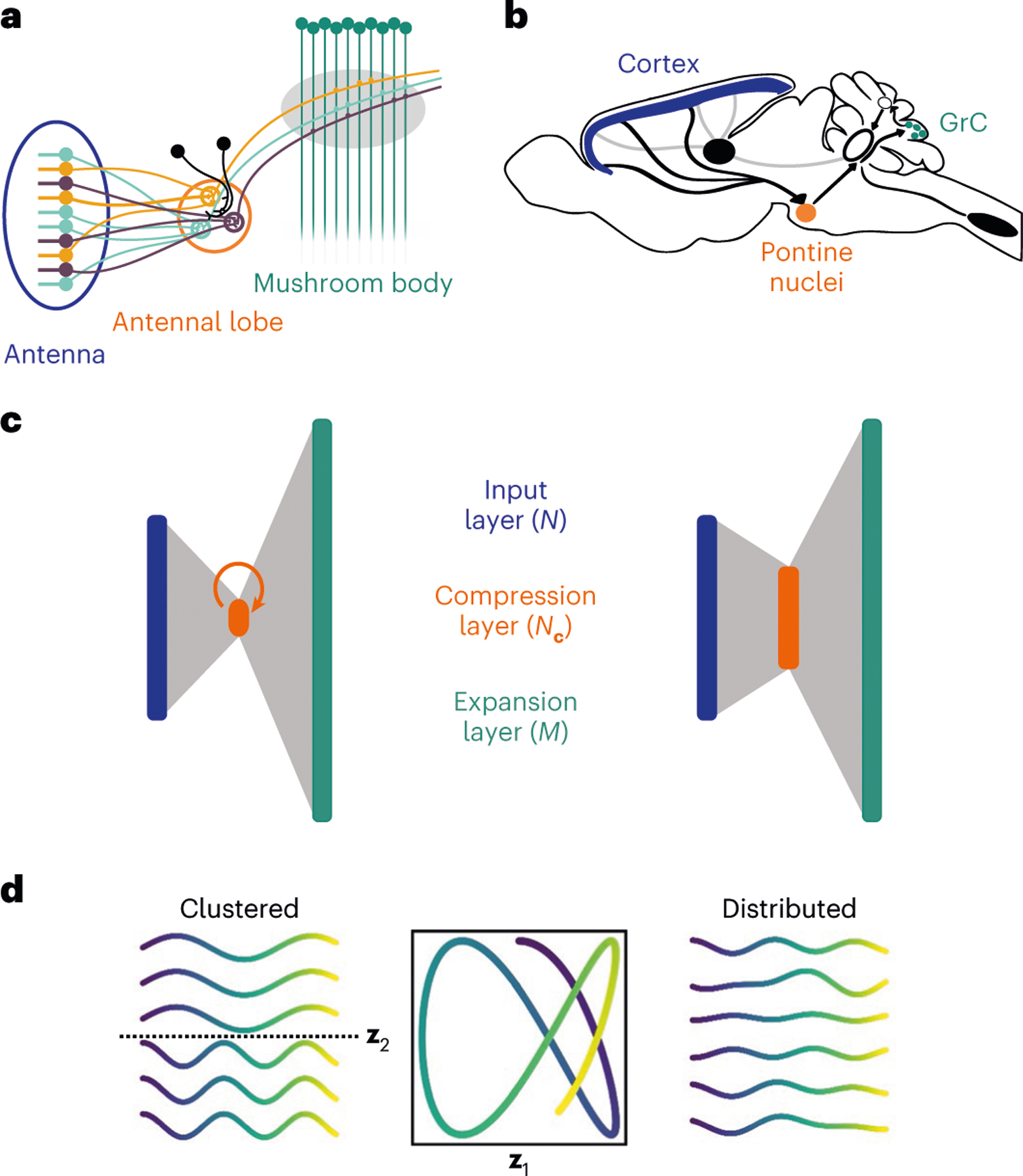
a, Schematic of the architecture of the insect olfactory system. Colors indicate OSNs in the antenna and glomeruli in the antennal lobe corresponding to specific olfactory receptor types. b, Schematic of the corticopontocerebellar pathway. c, Diagrams of neural network models of the insect olfactory system (left) and corticocerebellar pathway (right). The insect olfactory system is characterized by structured convergence to a compression layer that exhibits recurrent interactions among compression layer neurons. The corticopontine compression is less pronounced and the pontine nuclei have little-to-no recurrent connections. d, Example of clustered and distributed input representations. A smooth trajectory $\mathbf{\text{z}}$ in a two-dimensional task space (center) is embedded in an input representation of six neurons. Left, examples of input neuron responses in a clustered representation (each row is a neuron). Dotted line separates the two clusters. Right, examples of input neuron responses in a distributed representation.

While the pathways to cerebellum-like structures share this bottleneck architecture, the details of their microcircuitry differ. In the olfactory system of Drosophila (Fig. 1a) tens of olfactory receptor neurons expressing the same receptor project to an individual glomerulus in the antennal lobe¹⁴, which typically contains two projection neurons^15,16. In contrast, the corticocerebellar pathway (Fig. 1b) exhibits a less structured and less pronounced compression, with the ratio of the number of incoming fibers from the cerebral cortex to the number of neurons in the pontine nuclei estimated to be between two and ten⁷. Furthermore, while the pontine nuclei seem to have no lateral excitation and little-to-no lateral inhibition⁷, in the antennal lobe local neurons mediate effectively recurrent interactions among glomeruli^17,18 (Fig. 1c).

In contrast to neurons in expansion layers, which typically emit sparse bursts of action potentials^19,20, neurons in compression layers typically have higher firing rates^12,21. For this reason, in our model we consider either linear or rectified linear neurons for the compression layer, while for most of our results we use binary neurons to model the expansion layer (Methods). For a linear, feedforward compression, the activity of compression layer neurons is

$$\mathbf{c}=G^{\text{FF}}\mathbf{x},$$ (1)

where $G^{\text{FF}}$ represents feedforward connections from the input to compression layer. We also model recurrent connections within the compression layer with a matrix $G^{\text{rec}}$. In this case, compression layer activity evolves according to linear dynamics with a steady-state response to an input $\mathbf{x}$ given by (Methods)

$$\mathbf{c}={\left(I-G^{\text{rec}}\right)}^{-1}{G}^{\text{FF}}\mathbf{x}.$$ (2)

The activity of the expansion layer is

$$\mathbf{m}=\Theta (J\mathbf{c}-\mathit{\theta }),$$ (3)

where $J$ represents connections from the compression to expansion layer, $\Theta$ is the Heaviside step function and $\mathit{\theta }$ represents the firing thresholds of the expansion layer neurons. To mimic the random and sparse connectivity of the expansion in cerebellum-like structures, we assume that $J$ is a sparse random matrix with $K$ nonzero elements per row, representing $K$ connections onto each expansion layer neuron (Methods).

In our model, the network learns a mapping from patterns in a $D$-dimensional task subspace of the input layer activity to the target activation of a readout of the expansion layer, with $D\ll N$. This contrasts with previous work^4,5 that has typically assumed high-dimensional, random and uncorrelated input patterns. The task subspace represents the portion of the input space where inputs relevant to the task tend to lie and reflects the fact that neural computations are often performed in low-dimensional subspaces of the full activity space²². For example, OSNs of the same type respond similarly, thus defining a subspace in the space of all possible receptor firing rates. In addition to task-relevant activity, the input layer also includes task-irrelevant activity, which may lie both within and outside the task subspace.

We consider two classes of input representations, corresponding to different organizations of selectivities of input neurons to the task variables. In a clustered representation, input neurons belong to distinct groups, each of which is selective to a specific task variable (Fig. 1d, left). Such a representation can arise from a ‘labeled line’ wiring organization and leads to high within-group correlations. In contrast, in a distributed representation, each neuron is tuned to different linear combinations of multiple task variables (Fig. 1d, right). Our central contribution is a theory that relates these two classes of input representation to predictions about the compression architecture that optimizes downstream learning by the expansion layer.

Selectivity to task-relevant dimensions determines learning performance

To investigate the properties of this compression architecture, we begin with a standard benchmark: the ability of a readout of the expansion layer representation (for example, a Purkinje cell in the cerebellar cortex) to learn a categorization task using Hebbian plasticity. In such a task, $P$ input layer patterns are randomly associated with positive or negative labels (which could represent positive and negative valences associated to different conditioned stimuli^4,5). We compared the performance of a network without a compression layer, in which expansion layer neurons randomly sample input layer neurons (single-step expansion), with two networks with compression, specifically networks with either random or learned compression weights. Learned compression weights are trained using error backpropagation²³ (Methods). There is a substantial performance improvement from learning the compression weights, even though the subsequent expansion is fixed and random (Fig. 2a). However, the network with random compression performs worse than the network without compression (Fig. 2a). These results suggest that compression can be highly beneficial, but only if the compression weights are appropriately tuned. Furthermore, the benefit of compression is absent when the task-relevant representation is high-dimensional $(D=N)$ and unstructured, as considered in previous theories^4,5 (Extended Data Fig. 1b).

Fig. 2 |. Selectivity to task-relevant dimensions determines learning performance.

a, Fraction of errors of a Hebbian classifier on a random classification task (Methods). Learned compression indicates the performance when training via gradient descent has converged (Extended Data Fig. 1a). For each network, performance is averaged across ten noise realizations. $P$ values and $t$-statistics (two-sided Welch’s $t$-tests): random versus single-step expansion, $t=6.4,P={10}^{-5}$; single-step expansion versus learned compression, $t=8.5,p=3.5\times {10}^{-6}$; learned versus whitening compression, $t=2.6,P=0.018$. Parameters: $p=1$ (decay speed of task-relevant dimension variances), $N=500,N_{\text{c}}=D=P=50,M=\mathrm{2,000},K=4,f=0.1,\sigma =0.1$. Box plots show variability across network initializations, with the boundary extending from the first to the third quartile of the data. The whiskers extend from the box by 1.5 times the interquartile range. The horizontal line indicates the median. b, Dimension (top) and noise (bottom) for one example realization of random, learned and whitening compression strategies, as in a. Bar colors are matched to network diagram on the left. c, Fraction of errors of a Hebbian classifier on a random classification task, as a function of the input noise s.d. $\sigma$. Dots indicate simulation results (averaged across 40 simulations), lines indicate theoretical predictions. Dotted vertical lines indicate the range of $\sigma$ for which the performance of the compression strategy in which the compression layer units are tuned to task-relevant PCs (PC-aligned) and that of whitening compression are not significantly different (two-sided Welch’s $t$-test, $n=40$, criterion: $P<0.05$). The value of $p$ was increased to $p=1.5$ in this panel to make this trade-off more apparent. Other parameters: $N=500,N_{\text{c}}=D=P=50,M=\mathrm{2,000},K=4,f=0.1$.

We developed a theory to determine how compression connectivity shapes the expansion layer representation and affects task performance. The theory shows that a structured compression layer increases performance both by increasing the dimension of the expansion layer representation and by decreasing the noise, compared with random compression (Fig. 2b; Methods). Furthermore, it demonstrates that, for a linear compression layer, learning performance is maximized when compression layer neurons extract the task-relevant principal components (PCs) of the input representation (Methods). Beyond tuning to task-relevant inputs, compression layer neurons could adjust their gains to amplify subleading PCs, thereby increasing dimension. Consistent with this, a network in which all task-relevant PCs are equally strong in the compression layer (whitening compression) performs slightly better than networks whose compression weights are trained with backpropagation (Fig. 2a). However, a flexible biological implementation of whitening compression may require more complex machinery than tuning to task-relevant PCs without whitening, such as lateral inhibition or intrinsic plasticity at the compression layer. Furthermore, we find a trade-off between maximizing dimension by whitening and denoising: amplification of subleading PCs also amplifies noise (Methods), and whitening ceases to be the best strategy above a certain noise intensity (Fig. 2c). We refer to the network that optimizes the trade-off between dimension and noise as an optimal compression network.

Optimal compression for clustered and distributed representations

Because optimal compression reflects the statistics of the input, its properties differ substantially for clustered and distributed input representations. For a clustered representation, task-relevant PCs correspond to groups of similarly tuned neurons, whereas for a distributed representation they correspond to patterns of activity across the input layer (Fig. 3a,b). Selectivity of the steady-state compression layer neuron responses to task-relevant inputs requires that the rows of the matrix ${\left(I-G^{\text{rec}}\right)}^{-1}{G}^{\text{FF}}$ span the task subspace (equation (2); Methods). We study the case in which $G^{\text{FF}}$ contains only nonnegative elements, representing excitatory feedforward connections onto compression layer neurons (Fig. 1c).

Fig. 3 |. Optimal compression for clustered and distributed representations.

a, Illustration of input PCs for a clustered representation as in Fig. 1d. In the corresponding PC-aligned compression, clusters encoding the same task variable project to the same compression layer neuron (right). b, Same as a, but for a distributed representation. c, Top, example of covariance matrix for a clustered representation. Center, optimal compression matrix whose rows are proportional to the PCs of the above covariance matrix. Bottom, factorization of the optimal compression matrix as a square matrix multiplying a block rectangular matrix. d, Top and center are analogous to c, but for an example of a distributed representation. Bottom, example of a learned purely excitatory compression matrix that approximates the optimal compression matrix in the center panel. e, Results of gradient descent training when compression weights were constrained to be nonnegative (blue), compared with optimal compression (green), for a clustered input representation. Weights were trained to maximize dimension at the compression layer $\text{dim}\left(\mathbf{c}\right)$ while simultaneously minimizing noise (Methods). Top, normalized dimension of the compression layer representation (mean across ten network realizations), as a function of the input redundancy $N/D$. Bottom, same as top, but for noise strength in the compression layer. Shading indicates s.d. across network realizations. f, Same as e, but for a distributed representation. Parameters: $D=N_{\text{c}}=P=50$, $M=\mathrm{2,000},K=4,f=0.1,p=1,\sigma =0.1$.

When the input representation is clustered and correlations across clusters are present, we show that both feedforward and recurrent processing are required to achieve this objective. In this scenario, the task-relevant input covariance matrix is a block matrix, with strong within-block correlations (Fig. 3c, top). The optimal compression matrix can be factored into a product of $G^{\text{FF}},$ a $N_{\mathbf{\text{c}}}\times N$ nonnegative block matrix that represents convergence of input clusters onto compression layer neurons, and a $N_{\mathbf{\text{c}}}\times N_{\mathbf{\text{c}}}$ matrix $W^{\text{opt}}$ that represents interactions within the compression layer, that is $\mathbf{c}=W^{\text{opt}}{G}^{\text{FF}}\mathbf{x}$ (Fig. 3c, center and bottom; Methods). Comparing this expression with equation (2), the recurrent interactions are related to $W^{\text{opt}}$ via

$${\left(I-G^{\text{rec}}\right)}^{-1}=W^{\text{opt}}.$$ (4)

When the responses of input neurons belonging to different clusters are uncorrelated, $W^{\text{opt}}=I$ and $G^{\text{rec}}=0$, meaning recurrence is absent. When different clusters are correlated, however, decorrelation via the lateral interactions summarized in $W^{\text{opt}}$ is needed.

We next consider distributed input representations (Fig. 3d, top). In this case, the optimal compression matrix will include positive and negative entries, corresponding to excitatory and inhibitory connections (Fig. 3d, center). We asked whether optimal compression could be well approximated using only excitatory feedforward compression weights. We used gradient descent to adjust the weights to maximize dimension and minimize noise at the compression layer (Fig. 3d, bottom, Methods). Surprisingly, when the input representation is distributed and redundant $(N\gg D)$, purely excitatory connections lead to a compression layer dimension comparable to optimal compression (Fig. 3f, top). This is because, in this scenario, there are, with high probability, input neurons that encode each possible combination of task variables. Thus, even when connections are constrained to be excitatory, compression layer neurons can represent each of these combinations, successfully reconstructing the task subspace. In agreement with this intuition, the learned compression matrix is sparse, despite not having introduced any explicit sparsity bias (Extended Data Fig. 2a). Furthermore, the distribution of the number of outgoing connections per input layer neuron is broader than expected by chance (Extended Data Fig. 2b), suggesting that some input neurons are more likely to be compressed than others.

While purely excitatory compression is less effective in filtering out input noise, this limitation can be compensated by increasing input redundancy (that is, making $N/D$ larger, see Fig. 3f, bottom). Thus, even in the absence of lateral inhibition, excitatory compression weights are sufficient to maximize classification performance at the readout for large $N/D$ (Extended Data Fig. 2c,d). This result stands in contrast to our previous conclusion for systems with clustered input representations, for which decorrelation via lateral inhibition is necessary and for which increasing input redundancy does not increase the number of task variable combinations encoded (Fig. 3e and Extended Data Fig. 2e,f)

In total, we find that recurrence is necessary to decorrelate clustered input representations, while it is dispensable for distributed input representations as long as input redundancy is sufficiently high. In subsequent sections, we relate this distinction to differences in architecture between the antennal lobe and pontine nuclei (Fig.1c).

Compression of clustered representations in the insect olfactory system

In the insect olfactory system, OSNs that express the same receptor send excitatory projections to the same olfactory glomerulus in the antennal lobe¹⁴ (Fig. 4a). In our model, this corresponds to a clustered input representation with one cluster per receptor type. Each OSN cluster converges to specific compression layer neurons in antennal lobe glomeruli–the next stage of odor processing. Within the antennal lobe, local neurons mediate lateral interactions between glomeruli, which are predominantly inhibitory^17,18. Mushroom body Kenyon cells randomly mix projections from the glomeruli, thereby forming an expanded representation of olfactory information^24,25. This architecture is consistent with our theoretical results, which require both excitatory, convergent compression connectivity and recurrent interactions in the compression layer (Fig. 3c,e).

Fig. 4 |. Compression of clustered representations in the insect olfactory system.

a, Schematic of the insect olfactory system, highlighting feedforward and lateral recurrent connectivity. KC: Kenyon cell. b, Eigenvalue spectrum of the compression layer covariance matrix when inputs are constructed using experimental recordings²⁶, with and without global inhibition (purple and blue, respectively). Inset, corresponding compression layer dimension. c, Left, odor classification performance using realistic input statistics (left). The horizontal gray bar indicates the range in which global inhibition leads to a significant performance improvement (two-sided Welch’s $t$-test, $P<0.05,n=200$). Shaded areas indicate the s.e.m. across 200 network realizations. Right, as left, but for fixed $N/D=200$. The black violin plot corresponds to a network with purely inhibitory recurrent connections trained using gradient descent to approximate optimal compression (optimal inhibition), while green shows the performance of optimal compression. $P$ values and $t$-statistics are results of two-sided Welch’s $t$-tests. Parameters: $N_{\text{c}}=D=P=24,M=\mathrm{2,000},K=7,g_l=50,f=0.1,\sigma =0.5$. The whiskers of the violin plots indicate the full range of the data. Note that the value of $D$ (and consequently $N_{\text{c}}$ and $P$) is set to match the experimental data available, while $\sigma$ is increased to reflect the high degree of noise in the OSNs. $P$ values and $t$-statistics (two-sided Welch’s $t$-tests): excitatory compression with versus without global inhibition, $t=4.2,P=2.85\times {10}^{-5}$; global inhibition versus optimal inhibition, $t=4.3,P=2.02\times {10}^{-5}$. NS, not significant.

We hypothesized that evolutionary and developmental processes optimize the connectivity of the antennal lobe to facilitate a readout of the Kenyon cell representation, and asked whether the relation between input statistics and recurrent connectivity in the compression layer given by equation (4) is compatible with the lateral inhibitory interactions in the antennal lobe. We reanalyzed experimental recordings of single odor receptors to different odorants²⁶ and found that the correlations among OSN types are more positive than expected by chance (Extended Data Fig. 3a–c). We show analytically that when these correlations are uniformly positive, global lateral inhibition across antennal lobe glomeruli in the model is sufficient for optimal compression (Methods). Consistent with this and with studies that propose interglomerular interactions perform pattern decorrelation and normalization^11,27, global inhibition considerably increases the dimension of the antennal lobe representation when using the recorded responses as input to our model (Fig. 4b), leading to improved performance in an odor classification task (Fig. 4c, left). However, correlations are not uniformly positive, suggesting that further improvement could be achieved by fine-tuning the connectivity to the detailed structure of the input covariance matrix. To test this, we used gradient descent to train $G^{\text{rec}}$, which was constrained to be nonpositive. Strikingly, the resulting networks performed as well as optimal compression, and significantly better than networks with global inhibition only (Fig. 4c, right). Future studies should analyze whether the specific structure of lateral connectivity in the antennal lobe is consistent with this role (Discussion).

In contrast to networks with specific convergence of OSN types onto glomeruli, a model in which OSNs are mixed randomly in the antennal lobe performs poorly (Fig. 4c, left). It may seem counterintuitive that such convergence is needed for optimal performance when antennal lobe responses are subsequently randomly mixed by Kenyon cells. Our theory illustrates that this difference is a consequence of both denoising and maximization of dimension. When input neuron responses are noisy, pooling neurons belonging to the same cluster reduces noise by a factor $N/D$ compared with random compression (Methods). Even in the absence of noise, the dimension of the compression layer is higher for optimal compression than for random compression, because the latter introduces random distortions of the input layer representation. This can only be avoided by ensuring that weights onto compression layer neurons are orthogonal, a more stringent requirement that cannot be assured by independent random sampling of inputs (Methods). In fact, a block-structured $G^{\text{FF}}$ is the only possible nonnegative weight matrix that has this property. We also found an additional, more subtle benefit of glomerular convergence when considering sparse expansion layer connectivity (Extended Data Fig. 3d–g).

The factorization of the optimal compression connectivity into sparse feedforward convergence and dense recurrent interactions also requires fewer resources than a single feedforward compression matrix. In general, the purely feedforward strategy requires $N\times N_{\mathbf{\text{c}}}$ connections to be specified, while the factorized one requires $N+N_{\mathbf{\text{c}}}^2$ connections if recurrent interactions are monosynaptic. For the antennal lobe, the number of OSNs is $N\simeq \mathrm{1,200}$, the number of uniglomerular projection neurons is $N_{\mathbf{\text{c}}}\simeq 150$ and interactions between glomeruli are mediated by a population of $\simeq 200$ local neurons²⁸. This corresponds to 180,000 versus 61,200 connections for the purely feedforward and factorized strategies, respectively.

In total, our theory reveals that the glomerular organization of the antennal lobe optimizes the Kenyon cell representation for downstream learning. Moreover, for realistic input statistics, optimal compression is well approximated by a combination of feedforward excitation and lateral inhibition within the compression layer, consistent with antennal lobe anatomy.

Compression of distributed representations in the corticocerebellar pathway

In the corticocerebellar pathway, inputs from motor cortex are relayed to cerebellar GrC via a compressed representation in the pontine nuclei (Fig. 5a). The motor cortex representation is distributed across neurons^22,29, unlike the clustered representation of inputs to the antennal lobe. As we have shown earlier, optimal compression of distributed representations can be well approximated using only excitatory weights (Fig. 3f). This constraint seems to be required, because corticopontine projections are excitatory and the pontine nuclei lack strong inhibition. In rodents, recurrent inhibition seems to be completely absent, whereas for primates and larger mammals, it seems to play only a limited role⁷.

Fig. 5 |. Compression of distributed representations in the corticocerebellar pathway.

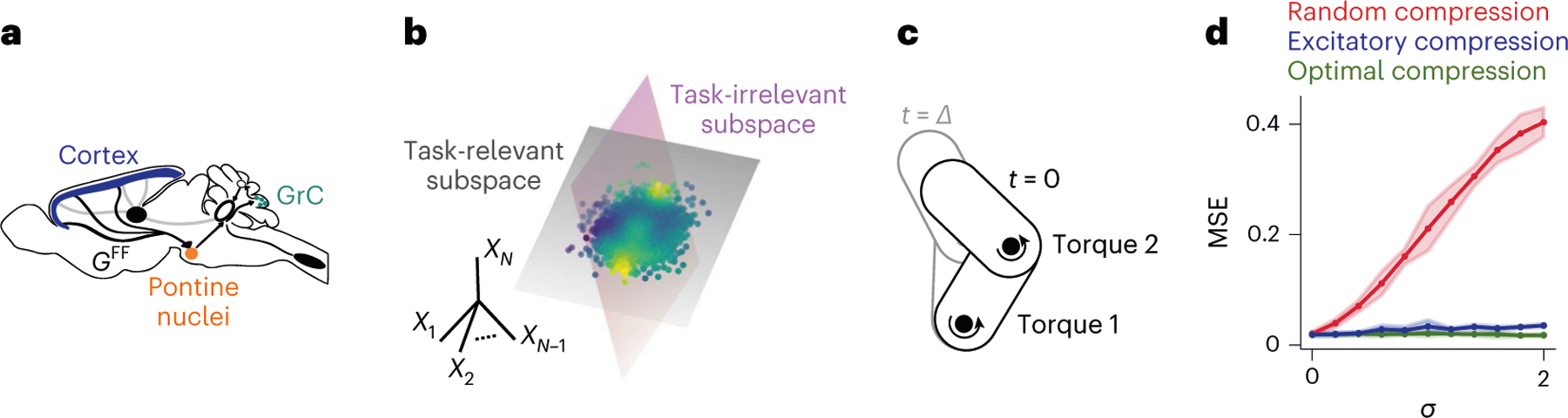
a, Schematic of the corticopontocerebellar pathway, highlighting the feedforward compression connectivity. b, Illustration of a continuously varying target. The high-dimensional cortical representation consists of orthogonal task-relevant and task-irrelevant subspaces. The cerebellum learns to map cortical activity (dots) to an output (color code) via a smooth nonlinear function. c, Schematic of two-joint arm task. Given joint angles, angular velocities, and torques $(D=6)$ at $t=0$, the system predicts the state of the arm at $t=\Delta$. d, MSE for the two-joint arm task, plotted against the strength of task-irrelevant activity $\sigma$. Optimal and excitatory compression perform significantly better than random compression when $\sigma \ge 0.2(P<0.05$, two-sided Welch’s $t$-test, $n=10)$. Optimal compression performs significantly better than purely excitatory compression only when task-irrelevant components are very strong (that is $\sigma \ge 1$, two-sided Welch’s $t$-test, $P<0.05,n=10)$. Low-dimensional task-irrelevant activity was generated as detailed in Methods, with $D_n=100$ and $p_n=1$. Network parameters: $N=500,N_{\text{c}}=100,M=\mathrm{2,000},f=0.3$. Task parameters: $\Delta =0.4\text{s},P_{\text{train}}=\mathrm{10,000}$. The coding level was increased compared with the classification task to match the higher optimal coding level observed in regression tasks⁵⁸. The solid lines and shaded areas indicate the mean and s.d. of the MSE across network realizations, respectively.

So far, we have focused on optimizing performance for a classification task. Some of the tasks that the cerebellum is involved in, such as eye-blink conditioning, may be reasonably interpreted in this way, but others may not. An influential hypothesis is that the cerebellum predicts the sensory consequences of motor commands, implementing a so-called forward model³⁰. In this view, the cerebellum integrates representations of the current motor command and sensory state to estimate future sensory states. We cast the problem of learning a forward model as a nonlinear regression task, assigning each point in the task subspace (representing the combination of motor command $\mathbf{u}$ and sensory state $\mathbf{s}$) a predicted sensory state ${\mathbf{s}}^{\prime }=\mathbf{s}+f(\mathbf{s},\mathbf{u})$ (Fig. 5b; Methods). In this scenario, the goal of model Purkinje cells (PkCs) is to learn the nonlinear function $f(\mathbf{s},\mathbf{u})$. We considered a planar arm model, with two joints at which torques can be applied (Fig. 5c). To introduce task-irrelevant activity consistent with experimental observations^31,32, we added low-dimensional noise acting on distributed modes to the cortical representation (Methods). Both optimal compression and purely excitatory compression lead to substantially better performance than random compression when learning a forward model for this system, showing that the benefits we have described are not specific to discrete classification tasks (Fig. 5d).

Our results reveal that the distributed nature of the cortical representation yields an optimal compression architecture compatible with the lack of inhibition in the corticopontine pathway. This is a qualitatively different conclusion than for systems with clustered inputs, for which excitation alone is insufficient, and applies when the readout is trained to perform either classification or continuous control tasks.

Optimal in-degree of learned corticopontine compression

Activity in motor cortex is task-dependent and exhibits steady drift in the neurons representing stable latent dynamics^29,33. Unlike the genetically determined, clustered representation of OSNs, such activity thus has a covariance structure that changes over time. We therefore extended our theory from the case of fixed compression weights to learning of compression weights through experience-dependent synaptic plasticity.

Hebbian plasticity is a natural candidate for learning compression weights, because it enables downstream neurons to extract leading PCs of upstream population activity^34,35. In many models, recurrent inhibitory interactions among downstream neurons are introduced to ensure that each neuron extracts a different PC. Due to the lack of inhibition in the pontine nuclei, we asked whether sparsity of compression connectivity instead can introduce the necessary diversity among pontine neuron afferents to achieve high performance.

We assumed that each compression layer neuron has in-degree $L$ (that is, receives $L$ connections from the input layer), corresponding to $L$ nonzero elements for each row of $G^{\text{FF}}$ in random locations. When these weights are set using Hebbian plasticity (Methods), the performance of a classifier trained on the expansion layer representation depends nonmonotonically on $L$. Performance is poor for small $L$, increases quickly and finally decays slowly as $L$ becomes large (Fig. 6a, left). Our theory demonstrates that this behavior is a result of the trade-off between denoising and dimension. Noise strength at the expansion layer decays with $L$, thanks to a more accurate estimation of leading PCs (Fig. 6a, top right). On the other hand, dimension decreases with $L$ as compression layer neurons tend to extract similar components (Fig. 6a, bottom right). The value $L^{\star }$ that yields the best performance lies between 10 and 100 incoming inputs. $L^{\star }$ is affected only weakly by architectural parameters such as the number of input neurons $N$, compression layer neurons $N_c$, or expansion layer neurons $M$ (Extended Data Fig. 4b–d). Instead, it depends on features of the input representation, with stronger noise favoring large in-degrees, and higher-dimensional representations leading to an increasingly pronounced optimum (Fig. 6b,c). In contrast to optimal compression, which requires only $N_{\mathbf{\text{c}}}=D$ compression layer neurons, Hebbian compression requires larger $N_{\mathbf{\text{c}}}$ (Extended Data Fig. 4a). This suggests that the smaller compression ratio of $N/N_c\approx 2-10$ for the corticopontine pathway, compared with $N/N_{\mathbf{\text{c}}}\approx 24$ for the antennal lobe, may arise due to the requirements of Hebbian plasticity.

Fig. 6 |. Biologically plausible learned compression.

a, Fraction of errors (left) of a Hebbian classifier reading out from the expansion layer for Hebbian compression, as a function of the compression layer in-degree $L$. Dashed horizontal lines indicate random and optimal compression. Right, dimension expansion (bottom) and noise contributions to the network performance (top), where ${\Delta }_{\text{m}}$ indicates the noise strength at the expansion layer (Methods). b, Same as a, left, but for different input noise strengths $\sigma$. $\mathbf{c}$, Same as b, but for different input dimensions $D$. In a, b and $\mathbf{c}$ we used $N=500,N_{\text{c}}=250,M=\mathrm{1,000},D=P=50$, $p=0.1,f=0.1$ and $\sigma =0.5$ unless otherwise stated. $p$ was reduced to highlight the trade-off between denoising and dimension. d, Illustration of the DCN-pontine feedback (in red). PN, pontine nuclei. e, Feedback from DCN improves selection of task-relevant dimensions. MSE for the two-joint arm forward model task, as in Fig.5c,d, versus strength of task-irrelevant dimensions $\sigma (\sigma =1$ signifies that the magnitude of the leading task-irrelevant and task-relevant components are the same). Hebbian compression with DCN feedback performs significantly better than without for all values of $\sigma (P<0.05$, two-sided Welch’s $t$-test, $n=10)$, particularly when $\sigma >1$. Inset, variance explained by task-irrelevant components (violet), in decreasing order, for two example values of $\sigma$ (green star and orange diamond). Gray dashed line indicates variance explained by the leading task-relevant component. $L=50$; other parameters same as Fig. 5d. In all panels, the solid lines and shaded areas indicate the mean and s.d. of the performance across network realizations, respectively.

Thus, in the absence of recurrent inhibition in the compression layer, an intermediate in-degree maximizes performance. This is true not only for random classification, but also for nonlinear regression (Extended Data Fig. 5a), suggesting that the trade-off between denoising and dimension is present across tasks. Given the low-dimensional representations observed in recordings of motor cortex²², we predict that the optimal in-degree $L^{\star }$ of rodent pontine neurons should be between 10 and 100. To our knowledge, this in-degree has not been measured, but the large dendritic arbor of these neurons³⁶ suggests that it is much larger than the in-degree of GrC, consistent with our theory.

We also tested whether further improvement could be achieved when recurrent inhibition is present, using a recent model that implements a combination of Hebbian and anti-Hebbian plasticity^35,37. After learning, the compression layer exhibit a richer representation of task variables than without recurrent inhibition (Extended Data Fig. 4e,f). We therefore predict that species with more recurrent inhibition in the pontine nuclei may exhibit larger excitatory pontine in-degree.

Feedback from the deep cerebellar nuclei improves selection of task-relevant dimensions

One limitation of tuning the compression weights using Hebbian plasticity is that, being an unsupervised method, Hebbian plasticity extracts leading PCs, but not necessarily task-relevant ones. This is not a problem when noise is random and high-dimensional, since in this case the leading PCs are likely to be task-relevant. However, it can reduce performance when leading components are task-irrelevant^31,32. The anatomy of the corticocerebellar system suggests a solution to this problem: in addition to cortical input, the pontine nuclei also receive feedback from the deep cerebellar nuclei (DCN)–the output structure of the cerebellum³⁶ (Fig. 6d). Previous theories have largely ignored these connections. We provide a new interpretation of this motif and suggest that it provides a supervisory signal that aids the identification of task-relevant inputs.

To test this hypothesis, we extended our corticocerebellar model to include feedback from the network output to the compression layer, akin to the DCN-pontine projection. In the compression layer, this feedback is used solely as a supervisory signal for synaptic plasticity, that is, it is added as an input to the learning rule but does not affect the network dynamics (Methods). Both compression weights and readout weights are learned online using biologically plausible rules. Specifically, we augment Oja’s rule³⁴ to include supervisory DCN feedback and show that such plasticity is biased towards components of the input that correlate with the target and are therefore likely task-relevant (Methods).

We tested this mechanism in the two-joint arm forward model task considered above. To model strong task-irrelevant activity, similar to Fig. 5f, we introduced low-dimensional noise acting on distributed modes with a decaying PC spectrum. When such noise is weak, Hebbian compression performs well, both with and without feedback (Fig. 6e). In contrast, when task-irrelevant components are stronger than task-relevant ones (Fig. 6e, inset), performance in the absence of feedback quickly degrades, as compression layer neurons learn to extract task-irrelevant components. Supervisory feedback alleviates this problem and improves performance (Fig. 6e, Extended Data Fig. 5b). This happens thanks to a rapid decrease of the error due to fast, online learning of the readout weights. Such relatively fast learning brings the network output close enough to the target to supervise learning of the compression weights (Extended Data Fig. 5c). In summary, our results support a new functional role for DCN projections to pontine neurons: enabling the extraction of task-relevant, but subleading, input components.

Hebbian compression can explain correlation and selectivity of GrC

Classic Marr–Albus theories of cerebellar cortex propose that the GrC representation should be as decorrelated and high-dimensional as possible, and that this is achieved by randomly mixing high-dimensional inputs^4,38. Our results argue that, for behaviors that can be represented in terms of a small set of task variables, it is beneficial for a bottleneck layer to extract only these variables. Recent recordings have shown that cerebellar GrC in mice exhibit high selectivity to task variables and strongly correlated activity, both with each other and with cortical neurons¹³, and this has been taken as evidence against Marr–Albus theories. We show that optimal compression in the corticopontine pathway provides an alternative explanation for these experimental findings that preserves mixing in the GrC layer.

We developed a model based on simultaneous two-photon calcium recordings of layer-5 pyramidal cells in motor cortex and cerebellar GrC¹³ (Fig. 7a). During recording sessions, mice performed a skilled forelimb task (Methods) that required them to move a joystick in a L-shaped trajectory, turning either to the left or right. We used recorded calcium traces of layer-5 pyramidal cells as inputs to the corticopontocerebellar model described above. In the model, corticopontine synapses undergo unsupervised learning via Hebbian plasticity. Similar to Wagner et al.¹³, we modeled unrecorded neurons by including an unobserved layer-5 population and a corresponding pontine subpopulation. The latter projects to both the observed GrC layer and to unobserved GrC not included in the model (Fig. 7b).

Fig. 7 |. Bottleneck model can explain correlations and selectivity of recorded GrC.

a, Illustration of the experimental design of Wagner et al.¹³. Mice performed a forelimb control task (left) while layer-5 pyramidal neurons and cerebellar GrC were recorded simultaneously using two-photon calcium imaging (right). Reproduced with permission from Wagner et al.¹³. b. Schematic illustrating how the bottleneck model is extended to reproduce the data. The dashed line indicates little or no mixing in the corticopontine pathway, while the shaded areas indicate strong mixing in the pontocerebellar pathway. c, Layer-5-GrC (magenta) and GrC–GrC (cyan) correlations, both in the data (dashed lines) and in the model (solid lines), for Hebbian (left) and random (right) compression strategies. Mean correlations across neurons are averaged across animals and plotted against ${\sigma }_N^{\text{uo}}$, the noise strength in the unobserved population. The colored shaded area indicates s.e.m., computed across animals. The gray shaded area indicates the region in which correlations in the model are not statistically different from those in the data for both areas $(P>0.05$, two-sided Wilcoxon signed-rank test; $n=10$). For this panel, the signal strength of the unobserved population is ${\sigma }_S^{\text{uo}}=1$. d, Average selectivity to left (L) and right (R) turns of the joystick, or to turns without direction preference (B), for GrC in the data (black), and models (Hebbian, blue; random, red). Selectivity is measured separately for the time window before (left) and after (right) the turn. Boxes indicate 25th and 75th percentiles across mice, while whiskers indicate the full range of the mean selectivities across mice. Asterisks indicate cases in which model and data are not compatible, color-coded according to the compression type (criterion, $P<0.05$; two-sided Wilcoxon signed-rank test; $n=10$). The box boundary extends from the first to the third quartile of the data. The whiskers extend from the minimum to the maximum of the data. The horizontal line indicates the median. In $\mathbf{d},{\sigma }_S^{\text{uo}}=1$ and ${\sigma }_N^{\text{uo}}=0.7$ for the Hebbian model and ${\sigma }_N^{\text{uo}}=0.1$ for the random model. For all panels, $N_{\text{c}}=N/2,M=10N,N_{\text{uo}}=2N,f=0.1,L=15$.

Since we do not have access to the unobserved population, we introduce two model parameters ${\sigma }_S^{\text{uo}}$ and ${\sigma }_N^{\text{uo}}$, which control the strength of task-relevant and task-irrelevant components of the unobserved cortical population (Methods). We systematically varied both parameters and measured average correlations in the model, both among GrC and between granule and layer-5 cells. The model and data are compatible using both measures, provided that task-irrelevant activity in the unobserved cortical population is strong enough (Fig. 7c, left). Notably, a model with random, nonplastic compression weights is not compatible with the data and exhibits lower correlations even for very small ${\sigma }_N^{\text{uo}}$ (Fig. 7c, right).

We also quantified the selectivity of model GrC subpopulations responsive to left and right turns of the joystick, or responsive to both directions, before and after the turn¹³ (Methods). When the parameters of the unobserved population were set so that correlations in the model fit those in the data, the model could also account for the observed selectivities (Fig. 7d). A model without Hebbian compression can also explain the selectivity profile, but only if task-irrelevant activity in the unobserved population is extremely weak.

Our analysis shows that the results of Wagner et al.¹³ are consistent with GrC responding to mixtures of mossy fiber activity. Due to Hebbian plasticity, pontine neurons in our model filter out task-irrelevant activity, becoming more selective to task variables and forming a lower-dimensional representation than would be expected from random compression. This decrease in dimension is not detrimental, but rather a consequence of discarding high-dimensional, task-irrelevant activity and preserving task-relevant activity. Since the latter is low-dimensional, random mixing at the model GrC layer yields only a moderate dimensional expansion and high correlations. Altogether, our results show that structured compression and random mixing of low-dimensional task variables, consistent with our theory of optimal compression, can account for the statistics of recorded responses.

Bottleneck architecture is more efficient than a single-step expansion

Throughout, we have assumed that the expansion connectivity is random. Because optimal compression, as we have defined it so far, involves a linear transformation, it is possible to generate a network with a single-step expansion that is equivalent to a two-step optimal compression network (Fig. 8a). This would yield a nonrandom expansion, with a synaptic weight matrix given by the product of the two-step compression and expansion weight matrices. What then is the advantage of performing these operations in two distinct steps? The answer is a consequence of the sparsity of the expansion layer weights.

Fig. 8 |. Comparison between bottleneck architecture and single-step network.

a, Single-step expansion (left) and optimal compression (right) architectures. Inset, illustration of local decorrelation at the expansion layer in the single-step expansion architecture. With sparse connectivity, each expansion layer neuron only has access to a subsampled version of the full input covariance matrix (three-by-three in the illustration). b, Fraction of errors (mean across 100 network realizations) in a random classification task for different network architectures plotted against the network expansion ratio. Local decorrelation does not significantly improve performance for small expansion layer neuron in-degree ($k=4$ shown; two-sided Welch’s $t$-test, $n=100$). Shaded areas indicate s.d. across network realizations. c, Similar to b, but plotted against $K$. The local decorrelation model performs significantly worse than optimal compression until $K=350$ (two-sided Welch’s $t$-test, $p<0.05,n=100$). In b and c, $N=500$, $N_{\text{c}}=D=50,P=50,M=\mathrm{2,000},K=4,f=0.1,p=1$, and $\sigma =0.1$, unless otherwise stated. d, Fraction of errors plotted against total number of synapses in the bottleneck architecture with local decorrelation at the compression layer (blue) and in a single-step expansion architecture with local decorrelation at the expansion layer (gray). Total synapse number was varied by changing $K$ or $L$ while keeping other parameters fixed. When the total number of synapses is 1 million, $P<{10}^{-10}$, two-sided Welch’s $t$-test, $t$-statistics $=15.468,n=40$. Parameters: $N=\mathrm{14,000},N_{\text{c}}=\mathrm{7,000},D=P=50,M=\mathrm{200,000},f=0.1,p=1,\sigma =0.1$. e, Same as d, but plotted against the pontine in-degree $L$ for the bottleneck architecture (left) and against the model GrC in-degree $K$ for the single-step expansion architecture (right). In d and e, the solid lines and shaded regions indicate the mean and s.e.m. across network realizations, respectively.

For a single-step expansion to implement both optimal compression and dimensional expansion, neurons in the expansion layer must be equipped with a local decorrelation mechanism across their afferent synapses (Fig. 8a, inset; Methods). However, due to their sparse connectivity, individual neurons receive input only from a subset of input neurons. Minimizing correlations within this subsampled representation will not, in general, lead to decorrelation of the full representation, since a whitening transformation requires knowledge of the global covariance structure. As a result, adding local decorrelation to a single-step expansion architecture does not yield a significant benefit if expansion layer neurons have small in-degrees and are not permitted to use nonlocal information (information about neurons to which they are not connected) to set synaptic weights (Fig. 8b).

If the expansion layer in-degree is increased, local decorrelation better approximates optimal compression (Fig. 8c). However, the total number of synapses necessary to implement this single-step architecture is much higher than for the two-step architecture. The wiring cost of performing local decorrelation at the expansion layer is particularly high when considering parameters consistent with cerebellar cortex, $M\simeq \mathrm{200,000}$ and $N_{\mathbf{\text{c}}}\simeq \mathrm{7,000}$ (Marr³;Fig. 8d,e). With local decorrelation at the compression layer, performance saturates when the compression in-degree $L$ is around 30 (Fig. 8e, left), totaling slightly more than a million synapses. For a network without a compression layer and with expansion layer neurons that perform local decorrelation, the performance is much worse if the total number of synapses is equalized (Fig. 8d). To achieve the same performance as the two-step architecture, the expansion in-degree would need to be between 10 and 20 (extrapolating from Fig. 8e, right), totaling between 2 and 4 million synapses. We reach a similar conclusion when considering parameters consistent with the insect olfactory system (Extended Data Fig. 6).

So far, we have assumed that the responses of the compression layer neurons are linear, meaning that the dimension of the compressed representation cannot be larger than $D$. Introducing a nonlinearity at the compression layer increases the expansion layer dimension, potentially improving input discriminability (Extended Data Fig. 7; Methods). We therefore asked whether two layers of nonlinear neuronal responses can further improve performance. Surprisingly, in our setting with nonlinear compression followed by random nonlinear expansion, we find that they cannot. This is because the compression nonlinearity amplifies noise, overwhelming the moderate increase in dimension. The fact that responses in the antennal lobe and pontine nuclei are substantially denser than those of Kenyon cells or GrC is consistent with these neurons operating closer to a linear regime²¹. In total, our results show that a dedicated compression layer with approximately linear responses provides an efficient implementation of optimal compression, both in terms of number of synapses and wiring complexity.

Discussion

Our results demonstrate that specialized processing in ‘bottleneck’ structures presynaptic to granule-like expansion layers substantially improves the quality of expanded representations. This two-step architecture, with a structured bottleneck followed by a disordered expansion, is also more efficient, in terms of total number of synapses, than a single-step expansion. The circuitry that optimizes performance depends on input statistics, with clustered and distributed input representations leading to different predictions about compression architecture.

Bottleneck architectures have been studied extensively in other contexts, such as compressed sensing³⁹, efficient coding^40–42 and autoencoders^43,44. In some cases, the relation between input statistics and the compressed representation has been studied^44,45. However, in the case of autoencoders and compressed sensing, the goal of the expansion layer is assumed to be input reconstruction, while for other theories only linear computation was considered⁴⁵. In contrast, our study highlights the importance of upstream compression in light of downstream nonlinear computation by the expansion layer. Furthermore, by studying inputs that may be low-dimensional, we generalize previous approaches that consider only random high-dimensional inputs^4,5, for which compression does not yield a benefit.

Other pathways to the cerebellum and other cerebellum-like structures

We focused on the corticopontocerebellar pathway and the insect olfactory system as the statistics of their inputs are better understood, but other pathways to the cerebellum and cerebellum-like structures also exhibit bottleneck architectures. Another main source of input to the cerebellum is the spinocerebellar pathway, which carries proprioceptive input from the spinal cord⁴⁶. In the dorsal spinocerebellar pathway, neurons in Clarke’s column relay lower limb proprioceptive inputs from muscle spindles and tendon organs to the cerebellum⁴⁷. Such neurons exhibit little convergence as they receive excitatory input from a single nerve. Interestingly, they also receive inhibitory inputs from other muscles. These observations suggest that the inputs to relay nuclei in the spinal cord exhibit clustered representations, which, according to our theory, benefit from inhibition from other clusters. Characterizing input statistics of this ensemble of proprioceptive inputs to predict the optimal organization of spinocerebellar pathways is an interesting direction for future research.

The electrosensory lobe of the electric fish is a cerebellum-like structure that exhibits synaptic plasticity required for cancellation of self-generated electrical signals⁴⁸. The nucleus praeeminentialis receives input from the midbrain and the cerebellum and projects solely to GrC in the electrosensory lobe². Interestingly, the nucleus praeeminentialis also receives feedback from the output neurons of the electrosensory lobe, analogous to DCN-pontine feedback connections⁴⁹. This suggests that our hypothesized supervisory role of DCN-pontine feedback could be an instance of a more general motif across cerebellum-like structures.

Response properties of compression layer neurons

Whereas in previous work¹³ pontine neurons have been modeled as binary, here we consider linear neurons, which we argue is more consistent with the graded firing rates they exhibit²¹. Indeed, pontine neurons have higher firing rates and denser responses than cerebellar GrC^12,19. Similar arguments apply to the insect olfactory system when comparing projection neurons to Kenyon cells²⁰. We tested that our results are consistent when pontine neurons are modeled using a rectified-linear nonlinearity and showed that nonlinear compression layer responses do not improve performance. This contrasts with nonrandom expansion architectures, such as deep networks, which can benefit substantially from multiple nonlinear layers¹, and reflects that a linear transformation is well-suited to maximize the performance of the subsequent random expansion. However, it is also possible that, for specific input statistics, nonlinear compression layer neurons lead to an improvement.

In our models, we have neglected intrinsic noise in compression layer neurons. Introducing such noise is mathematically equivalent to increasing the noise strength at the expansion layer (Methods), leaving our analysis of the biological architectures that realize optimal compression unchanged. Furthermore, while the level of intrinsic noise for compression layer neurons in cerebellum-like structures is not known, noise at the input layer is likely to be a dominant source of variability. Insect OSN responses are strongly affected by the variability of binding of the odorant to the odor receptor⁹, which is largely independent across neurons. As we showed, compression onto the glomeruli reduces this type of noise by a factor $N/D$. In the corticocerebellar pathway, the main source of noise is likely task-irrelevant activity that is distributed across cortical neurons^31,32.

At the population level, our theory predicts that compression layers should exhibit a larger proportion of task-relevant activity and more decorrelated representations. Previous studies have shown signatures of pattern decorrelation and normalization in the antennal lobe^10,27. Recordings in the pontine nuclei are challenging and only a small number of neurons have been recorded simultaneously. Population recordings of these neurons could distinguish whitening compression, which predicts that the principal component analysis (PCA) spectrum of the pontine population decays more slowly than that of layer-5 pyramidal cells, from nonwhitening compression.

Feedforward and lateral inhibition

The cholinergic projections of OSNs to the antennal lobe are excitatory⁵⁰. We showed that, when the input representation is clustered and correlations between clusters exist, either disynaptic feedforward or lateral inhibition is necessary to maximize performance. In the antennal lobe, both types of inhibition are present. However, disynaptic inhibition is believed to largely mediate interactions among different glomeruli¹⁰, suggesting that lateral inhibition dominates. We showed that global lateral inhibition is sufficient to effectively denoise and decorrelate OSNs whose response properties are constrained by experimental data²⁶.An interesting future direction is to investigate whether the detailed pattern of response correlations across glomeruli is reflected in their lateral connections⁵¹. However, such a prediction requires accurate estimation of this correlation pattern over the distribution of natural odor statistics, which may not be reflected in existing datasets.

In most mammalian brain areas, long-range projections are predominantly excitatory, and this is true of corticopontine projections from layer-5 pyramidal cells. While inhibitory disynaptic pathways to the pontine nuclei do exist^7,12, our results show, surprisingly, that purely excitatory compression weights can perform near-optimally when the input representation is redundant and distributed, rather than clustered. However, lateral inhibition might play a role in learning, promoting competition to ensure heterogeneous responses even when compression layer neurons share many inputs³⁵. While lateral inhibition is almost absent from the pontine nuclei in rodents, its prevalence increases in larger mammals, such as cats and primates⁷. In species where lateral inhibition is more abundant, pontine neurons may be more specifically tuned to task-relevant input dimensions and exhibit larger in-degrees.

Corticopontine learning and topographical organization of the pontine nuclei

Our theory highlights the importance of plasticity at corticopontine synapses, which permit pontine neurons to track slow changes of the task-relevant cortical input space. This could, for example, compensate for representational drift in motor cortex^29,33. We also showed that such subspace selection can be further improved by supervisory feedback from the DCN, a mechanism which is supported by the presence of particularly strong feedback projections from the dentate nuclei⁵², an area which is also heavily pontine-recipient. Alternatively, these feedback connections could gate different pontine populations or modes, enabling fast contextual switching⁵³. Another possibility is that part of the learning process that enables subspace selection is carried out by layer-5 pyramidal cells.

At a larger scale, the pontine nuclei exhibit a topographic organization, perhaps genetically determined, that largely reflects the cortical organization^54,55. For example, motor cortical neurons whose output controls different body parts project to distinct pontine regions. Moreover, there is evidence of convergence of motor and somatosensory cortical neurons coding for the same body part onto neighboring pontine regions⁵⁶. It is therefore likely that both hard-coded connectivity and experience-dependent plasticity control the compression statistics.

Random mixing and correlations in low-dimensional tasks

Our theory is consistent with data collected using simultaneous two-photon imaging from layer-5 pyramidal cells in motor cortex and cerebellar GrC¹³. We showed that the level of correlations and selectivity of GrC can be explained if corticopontine connections are tuned to task-relevant dimensions, but not if they are fixed and random. A previous theory proposed a model to account for this data in which, during the course of learning, mixing in the GrC layer is reduced and a single mossy fiber input comes to dominate the response of each GrC¹³. Our model preserves mixing in GrC–a feature thought to be crucial for cerebellar computation³, and instead emphasizes the role of low-dimensional GrC representations when animals are engaged in behaviors with low-dimensional structure. Such an interpretation may generally account for recordings of GrC that exhibit low dimensionality and suggests the importance of complex behavioral tasks or multiple behaviors to probe the computations supported by these neurons⁵⁷.

Methods

Network model

We model the input pathway to cerebellum-like structures as a three-layer feedforward neural network. The input layer activity $\mathbf{x}$ represents the task subspace (see below) and task-irrelevant activity. The representation $\mathbf{x}$ is sent to the compression layer via a compression matrix $G\in {ℳ}^{N_{\mathbf{\text{c}}}\times N}$. We consider both linear compression layer neurons, for which $\mathbf{c}=G\mathbf{x}$ and rectified linear unit (ReLU) neurons, for which $\mathbf{c}=[G\mathbf{x}-\mathit{\theta }{]}^{+}$, where the rectification is applied element-wise. The output of the compression layer is sent to the expansion layer via a matrix $J\in {ℳ}^{M\times N_{\mathbf{\text{c}}}}$, and we set $\mathbf{m}=\mathit{\varphi }(J\mathbf{c}-\mathit{\theta })$, once again applied element-wise. In our results, $\varphi$ is a Heaviside threshold function, except when considering nonlinear regression and when reanalyzing the data from Wagner et al.¹³, for which we used a ReLU nonlinearity. The nonzero entries of the expansion matrix $J$ are independent and identically distributed (i.i.d.) random variable, sampled from $𝒩(\mathrm{0,1}/K)$, where $K$ is the number of incoming connections onto an expansion layer neuron. The thresholds $\mathit{\theta }$ are chosen adaptively and independently for each neuron to obtain the desired coding level (fraction of active neurons) $f$ or $f_{\mathbf{c}}$ (ref. 4), for the expansion and compression layer, respectively. The expansion representation $\mathbf{m}$ is read out via readout weights $\mathbf{w}$, that is, the network output is ${\widehat{y}}^{\mu }={\mathbf{w}}^T(\mathbf{m}-f\mathbf{1})$, where $1$ indicates the vector of all ones. The readout weights are set using a Hebbian rule (Hebbian classifier), unless stated otherwise, that is

$$\mathbf{w}=\sum _{\mu =1}^P \left({\mathbf{m}}^{\mu }-f\cdot 1\right)y^{\mu },$$ (5)

where ${\text{y}}^{\mu }$ are the target labels.

Recurrent compression layer.

Recurrent interactions in the compression layer can be modeled via the differential equation

$${\tau }_{\mathbf{c}}\dot{\mathbf{c}}=-\mathbf{c}+G^{\text{rec}}\mathbf{c}+G^{\text{FF}}\mathbf{x},$$ (6)

where $G^{\text{rec}}$ is the matrix of recurrent interactions in the compression layer and $G^{\text{FF}}$ is the matrix of feedforward interactions from the input to the compression layer. We assume that ${\tau }_{\mathbf{c}}$ is much smaller than the time-scale at which the input varies, so that we can focus on the steady-state dynamics given by

$$\mathbf{c}=G^{\text{rec}}\mathbf{c}+G^{\text{FF}}\mathbf{x}\Rightarrow \mathbf{c}={\left(I-G^{\text{rec}}\right)}^{-1}{G}^{\text{FF}}\mathbf{X}=:G^{\text{eff}}\mathbf{x},$$ (7)

where we defined the effective feedforward matrix as $G^{\text{eff}}:={\left(I-G^{\text{rec}}\right)}^{-1}{G}^{\text{FF}}$. Therefore the compression matrix $G^{\text{eff}}$ can be thought as the effective steady-state compression matrix in the presence of recurrent interactions and linear neurons.

Single-step expansion network.

To compare the performance of the bottleneck network with one without the compression layer, we also implement a single-step expansion network, in which the input layer $\mathbf{x}$ is directly expanded to the expansion layer $\mathbf{m}$ via a sparse expansion matrix $J$, that is, $\mathbf{m}=\mathit{\varphi }(J\mathbf{x}-\mathit{\theta })$. The matrix $J\in {ℳ}^{M\times N}$ has $K$ nonzero elements per row, with these entries sampled as for the bottleneck network.

Input representation

We model the input representation $\mathbf{x}$ as a linear mixture of task-relevant and task-irrelevant activity (that is, noise). The task-relevant variables are described by a $D$-dimensional representation $\mathbf{z}$, and are encoded in the input layer via a matrix with orthonormal columns $A$. Similarly, the task-irrelevant activity is generated by embedding a $D_n$-dimensional, task-irrelevant representation ${\mathbf{z}}_n$ in the input layer using a matrix with orthonormal columns $A_n$. The input representation is therefore given by

$$\mathbf{\text{x}}=\sqrt{\frac{N}{D}}A\mathbf{\text{z}}+\sqrt{\frac{N}{D_n}}\sigma A_n{\mathbf{\text{z}}}_n=:\overline{\mathbf{\text{x}}}+\sigma \mathbf{\xi },$$ (8)

where $\sigma$ is a scalar parameter controlling the noise strength, $A^{T}A=I_D$, and analogously for $A_n$. The columns of $A$ can always be chosen to be orthonormal to each other, since we assume that $N\ge D$. For this reason, we also assume that $N\ge D_n$. The factors $\sqrt{\frac{N}{D}}$ and $\sqrt{\frac{N}{D_n}}$ ensure that input layer activity is of order 1. As we will describe in more detail, both $\stackrel{-}{\mathbf{x}}$ and $\mathit{\xi }$ are Gaussian vectors and uncorrelated with each other, therefore $\mathbf{x}$ is also Gaussian with covariance matrix $C^{\mathbf{x}}=\frac{N}{D}A{C}^{\mathbf{z}}{A}^T+{\sigma }^2\frac{N_n}{D_n}{A}_n{C}^{{\mathbf{z}}_n}{A}_n^T$.

Task-relevant representation.

The task variables $\mathbf{z}$ in equation (8) consist of $D$-dimensional random Gaussian patterns, sampled from $𝒩(0,\Lambda )$, where $\Lambda$ is a $D\times D$ diagonal matrix with diagonal elements ${\lambda }_1,\dots ,{\lambda }_D$. The $\left\{{\lambda }_i\right\}$ represent the task subspace PCA eigenvalues, and to control their decay speed we set ${\lambda }_i=i^{-p}$ and vary the parameter $p$.

The choice of the matrix $A$ determines the quality of the input representation. To model distributed input representations, we sample a random $N\times N$ orthogonal matrix $O_N$ from a Haar measure⁵⁹ (the analog of uniform measure for matrix groups), and select the first $D$ columns of $O_N$ to be the columns of $A$. To model clustered input representations, we split the $N$ input neurons into $D$ groups. For simplicity, we take these groups to be equally sized, that is each group consists of $N_g$ neurons, but our results can be easily generalized to the case of groups with different sizes. To include correlations among neurons belonging to different clusters, we set $A=B{O}_D$, where $O_D$ is a $D\times D$ orthogonal matrix sampled from a Haar measure. The elements of the matrix $B$ are set as

$$B_{ij}=\left\{\begin{array}{l}\sqrt{1/N_g}\text{if neuron }i\text{ belongs to group }j\\ 0\text{ otherwise}\end{array}\right.$$ (9)

Task-irrelevant activity (noise).

The task-irrelevant component $\mathit{\xi }$ of the input representation in equation (8), that is, the input noise, was generated analogously to the task-relevant one, that is ${\mathbf{z}}_n$ consisted of $D_n$-dimensional random Gaussian patterns, sampled from $𝒩\left(0,{\Lambda }_n\right)$, where ${\Lambda }_n$ is a diagonal matrix with elements ${\lambda }_i^n=i^{-p_n}$, for $i=1,\dots ,D_n$. For most of our analyses, we considered high-dimensional isotropic noise, that is $D_n=N,p_n=0$ and $A_n=I_N$. However, when analyzing the performance on the forward model task (Fig. 5d and Fig. 6e), we also considered lower-dimensional, distributed noise, because task-irrelevant activity in motor cortex seems to be relatively low-dimensional^31,32. In this case, we sampled $A_n$ from the Haar measure, analogously to $A$ for distributed task-relevant representations.

We also added noise at the expansion layer. The latter depended on the type of nonlinearity used at the expansion layer. For binary neurons, used for most of our results, we randomly flipped a fraction ${\sigma }_{\mathbf{\text{m}}}$ of the neurons for every pattern. For ReLU neurons, we added random isotropic Gaussian noise with variance ${\sigma }_{\mathbf{m}}^2$ after the rectification, while keeping the final rate positive. Noise could also affect the compression layer representation, but we can absorb this contribution into the noise at the expansion layer (as noise at the expansion layer increases monotonically with the noise at the compression layer; Supplementary Modeling Note).

Metrics of dimension and noise

To quantify the dimension of a representation, we use a measure based on its covariance structure^5,60. For a representation $\mathbf{x}$ with covariance matrix $C^{\mathbf{x}}$, which has eigenvalues ${\lambda }_1,\dots ,{\lambda }_n$, we define

$$\text{dim}\left(\mathbf{\text{x}}\right)≔\frac{\text{Tr}{\left(C^{\mathbf{\text{x}}}\right)}^2}{\text{Tr}\left({(C^{\mathbf{\text{x}}})}^2\right)}=\frac{{\left({\sum }_i{\lambda }_i\right)}^2}{{\sum }_i{\lambda }_i^2}.$$ (10)

In the absence of noise, and because of the orthonormality of the columns of $A$, the nonzero eigenvalues of $C^{\mathbf{x}}$ are equal to ${\lambda }_1,\dots ,{\lambda }_D$, that is, the PCA eigenvalues of $\mathbf{x}$ are the same as those of $\mathbf{z}$. Therefore, $\text{dim}\left(\mathbf{x}\right)=\text{dim}\left(\mathbf{z}\right)$. This can also be seen by noting that the columns of $A$ form an orthonormal set, that is $A^{T}A=I$, and using the cyclic permutation invariance of the trace, for any representation $\mathbf{z}$ with covariance matrix $C^{\mathbf{z}}$ (possibly nondiagonal):

$$\text{Tr}\left(C^{\mathbf{x}}\right)=\text{Tr}\left(A{C}^{\mathbf{z}}{A}^T\right)=\frac{N}{D}\text{Tr}\left(A^{T}A{C}^{\mathbf{z}}\right)=\frac{N}{D}\text{Tr}\left(C^{\mathbf{z}}\right),$$ (11)

and analogously $\text{Tr}\left({\left(C^{\mathbf{x}}\right)}^2\right)=\frac{N^2}{D^2}\text{Tr}\left({\left(C^{\mathbf{z}}\right)}^2\right)$. As a result, the factor $N/D$ simplifies and the dimension remains unchanged.

To quantify noise strength, we follow previous work and consider the Euclidean distance between a noiseless pattern $\stackrel{-}{\mathbf{x}}$ and a noisy pattern $\mathbf{x}$, specifically $d(\mathbf{x},\stackrel{-}{\mathbf{x}})={\sum }_{i=1}^N {\left({\mathbf{x}}_i-{\stackrel{-}{\mathbf{x}}}_i\right)}^2$ (ref. 4). This distance is averaged over the input and noise distribution and normalized by the average distance among pairs of noiseless input patterns, that is:

$${\Delta }_{\mathbf{x}}=\frac{{⟨d\left({\mathbf{x}}^{\mu },{\stackrel{-}{\mathbf{x}}}^{\mu }\right)⟩}_{\mu ,\xi }}{{⟨d\left({\stackrel{-}{\mathbf{x}}}^{\mu },{\stackrel{-}{\mathbf{x}}}^v\right)⟩}_{\mu }},$$ (12)

where $\mu$ denotes the average over the input distribution and $\xi$ the average over the noise distribution. With this normalization, ${\Delta }_x=1$ if noisy patterns are, on average, as distant from their noiseless version as two different input patterns are with respect to each other. The definition of ${\Delta }_{\mathbf{c}}$ and ${\Delta }_{\mathbf{m}}$ for the noise strength at the compression and expansion layer is analogous to that in equation (12).

Random classification task

A random classification task is defined by first assigning binary labels $y^{\mu }=\pm 1$ at random to patterns ${\mathbf{z}}^{\mu }$, for $\mu =1,\dots ,P$, in the task subspace. The network is required to learn these associations and generalize them to patterns that are corrupted by noise. When readout weights are learned using a Hebbian rule (equation (5)), the probability of a classification error can be expressed in terms of the signal-to-noise ratio (SNR) of the input received by the readout neuron, as $P\left(\text{error}\right)\simeq \frac{1}{2}\text{erfc}\left(\sqrt{\frac{\text{SNR}}{2}}\right)$ (ref. 4). Previous work⁵ has shown that the SNR can be expressed as

$$\text{SNR}\simeq \frac{\text{dim}\left(\stackrel{-}{\mathbf{m}}\right){\left(1-{\Delta }_{\text{m}}\right)}^2}{P},$$ (13)

where ${\Delta }_{\mathbf{m}}$ is the noise strength at the expansion layer (analogous to equation (12); Methods), while $\text{dim}\left(\stackrel{-}{\mathbf{m}}\right)$ is the noiseless dimension, that is, the dimension of the task-relevant expansion layer representation $\stackrel{-}{\mathbf{m}}$ (analogous to equation (10); Methods). Since we always consider the dimension of task-relevant representations, we lighten the notation by dropping the bar and writing $\text{dim}\left(\mathbf{x}\right),\text{dim}\left(\mathbf{c}\right),\text{dim}\left(\mathbf{m}\right)$, for the task-relevant input, compression, and expansion layer, respectively.

Compression architectures

Here, we briefly describe the different types of compression that we considered in the main text. We note that, when compression is linear, multiplying any of the compression matrices below by an $N_{\text{c}}\times N_{\mathbf{\text{c}}}$ orthogonal matrix has no effect on the dimension and noise strength of the compression layer. For the case of PC-aligned compression, however, a subtle advantage at the expansion layer is present when such additional rotation is absent (Extended Data Fig. 3d–g). In contrast, for nonlinear compression and $N_{\mathbf{\text{c}}}>D$, the additional rotation is beneficial as it increases the dimension of the compression layer after the nonlinearity.

Random compression.

We model random, unstructured compression by sampling the entries of the compression matrix $G$ i.i.d. from a Gaussian distribution, that is

$$G_{ij}^{\text{rnd}}~𝒩\left(0,\frac{1}{N}\right),$$ (14)

where the scaling of the variance is chosen to obtain order 1 activity in the compression layer.

PC-aligned compression.

For PC-aligned compression the rows of $G$ are set equal to the task-relevant PCs of the input. Since the task-relevant variables are embedded in the input layer via the orthonormal columns of $A$, the latter are the task-relevant PCs. Therefore,

$$G^{\text{PC}}≔\sqrt{\frac{D}{N}}{A}^T.$$ (15)

Once again, the scaling factor ensures that the activity of compression layer neurons are order 1. The above expression is valid when $N_{\mathbf{c}}=D$. If $N_{\mathbf{\text{c}}}>D$, we duplicate the rows of $G^{\text{PC}}$, which results in a clustered representation at the compression layer. Note that with this type of compression, the task-relevant activity in the compression layer is decorrelated, because the task-relevant covariance matrix is given by $C^{\text{c}}=\frac{D}{N}A{C}^{\text{x}}{A}^T=C^z$, which is diagonal by construction.

Whitening compression.

To obtain a whitened spectrum, the rows of $G^{\text{PC}}$ can be scaled in such a way that $C^{\text{c}}=I$. Since the eigenvalues of $C^{\mathbf{x}}$ are the same as the PCA eigenvalues of the task subspace representation $\mathbf{z}$, this is accomplished when:

$$G^{\text{W}}≔\sqrt{\frac{D}{N}}\text{diag}\left({\lambda }_1^{-1/2},\dots ,{\lambda }_D^{-1/2}\right)A^T.$$ (16)

Similar to PC-aligned compression, if $N_{\mathbf{\text{c}}}>D$, we duplicate the rows of $G^{\text{W}}$.

Optimal compression.

We define the optimal compression matrix as either $G^{\text{PC}}$ or $G^{\text{W}}$, depending on which leads to the best performance. For nearly all the regimes we consider, whitening leads to the best performance.

Optimization of compression weights via gradient descent.

For Fig. 2a,b, Fig. 3e,f and Extended Data Fig. 7c we used gradient descent to optimize the compression weights. We trained compression weights using backpropagation under the assumption that readout weights are learned using the Hebbian rule (equation (5)). More precisely, for each epoch we sampled a random sparse expansion matrix $J$ and $B=10$ random classification tasks, each consisting of $P=D=50$ target patterns.

For Fig. 2a and Extended Data Fig. 7c, Hebbian readout weights are set independently for each task, after which the compression weights are updated in the direction that decreases the loss (binary cross-entropy) computed on noise-corrupted test patterns. The update step was performed using the Adam optimizer⁶¹, with a learning rate $\eta ={10}^{-4}$. To facilitate learning by gradient descent, we replaced Heaviside nonlinearities in the expansion layer with ReLU nonlinearities. Adaptive thresholds were set, as in the rest of the paper, to obtain the desired coding level $f$. We used the same setup to test the performance in the presence of nonlinearities in the compression layer. We introduced ReLU nonlinearities in the compression layer in the same way as we did for the expansion layer, with a coding level $f_{\mathbf{\text{c}}}=0.3$.

For Fig. 3e,f, the compression weights were adjusted to approximate optimal compression by simultaneously maximizing dimension and minimizing noise at the compression layer. To achieve this, we chose as the objective function the maximization of ${\text{SNR}}_{\mathbf{c}}=\frac{\text{dim}\left(\mathbf{c}\right){\left(1-{\Delta }_{\mathbf{c}}\right)}^2}{P}$ (analogous to equation (13) for the compression layer). At every epoch, excitatory weights were constrained to be nonnegative.

Hebbian compression.

In Figs. 6 and 7, we considered biologically plausible learning of compression weights. In particular, we exploit the well known result that Hebbian plasticity leads to the postsynaptic neuron extracting the leading PC of its input³⁴. In the presence of sparse compression connectivity, a compression layer neuron receives input from $L$ input layer neurons. We call $S_i=\left\{j_1,\dots ,j_L\right\}$ the set of indices of input layer neurons that project to neuron $c_i$. The covariance $C_{kl}^{c_i}$ of such input is therefore a $L\times L$ matrix given by

$$C_{kl}^{c_i}=C_{j_k{j}_l}^{\mathbf{x}}\text{for}{j}_k,j_l\in S_i.$$ (17)

The leading PC of the input to neuron ${\text{c}}_i$ is the (normalized) eigenvector of $C_{kl}^{c_i}$ corresponding to its leading eigenvalue. Therefore, to mimic Hebbian plasticity in the presence of sparse connectivity, we set the $i$th row of $G$ to the leading eigenvector of $C_{kl}^{c_i}$. Notice that, for small $L$, the leading eigenvector of $C_{kl}^{c_i}$ might be substantially different from the leading eigenvector of the full covariance of the input $C^{\mathbf{x}}$. Therefore, sparse connectivity introduces diversity of tuning across compression layer neurons, at the cost of pushing the tuning vectors outside of the task subspace, resulting in stronger noise.

Derivation of optimal compression

A key result of our theory is that, when expansion weights are random, optimal compression requires compression layer neurons to be tuned to task-relevant input PCs. Furthermore, the gain of different compression layer neurons could be adjusted to further increase performance. However, to what degree it is convenient to do so depends on the input noise strength.

We start from the expression for the SNR of a Hebbian classifier (equation (13)), which is a proxy of classification performance on a random classification task⁴. To maximize the SNR, we would ideally maximize $\text{dim}\left(\mathbf{m}\right)$ while minimizing the noise ${\Delta }_{\mathbf{m}}$. We find that aligning the weights to the PCs favors both objectives, while performing additional whitening increases dimension but also noise. While performance depends on dimension and noise at the expansion layer, in most cases the dimension and noise at the compression layer is sufficient to explain the resulting performance. This is because (1) noise at the expansion layer is a monotonic function of noise at the compression layer (Supplementary Modeling Note and Extended Data Fig. 8) and (2) dimension of the expansion layer depends on the dimension of the compression layer (Supplementary Modeling Note and Extended Data Fig. 8). However, dimension can also depend on the fine structure of the compression layer representation, in particular when the expansion connectivity is sparse (Supplementary Modeling Note). Below, we show how the properties of compression weights determine dimension and noise at the compression layer, motivating our definition of optimal compression.

Effect of compression on dimension.

Here we present analytical results on the dimension of the compression layer in the case of linear compression. By definition of the dimension (equation (10)), we need to compute:

$$\text{dim}\left(\mathbf{c}\right)=\frac{\text{Tr}{\left(C^{\mathbf{c}}\right)}^2}{\text{Tr}\left({\left(C^{\mathbf{c}}\right)}^2\right)}$$ (18)

For random compression, it is convenient to reinterpret the trace as an average across compression layer neurons:

$$\text{dim}\left(\mathbf{c}\right)=\frac{N_{\mathbf{c}}{⟨C_{ii}^{\mathbf{c}}⟩}^2}{⟨{\left(C_{ii}^{\mathbf{c}}\right)}^2⟩+\left(N_{\mathbf{c}}-1\right)⟨{\left(C_{ij}^{\mathbf{c}}\right)}^2⟩},$$ (19)

where the average is intended over $i$ and $j$. We now define $\tilde{G}:=GA$, that is, the effective matrix transforming the task variables into the compression layer representation (up to a factor $\sqrt{N/D}$, which is irrelevant for the dimension). Since the columns of $A$ are orthonormal, the elements of $\tilde{G}$ are also normally distributed and independent, with mean zero and variance $1/N$. We have that $C_{ij}^{\mathbf{c}}={\sum }_{k=1}^D {\tilde{G}}_{ik}{\tilde{G}}_{jk}{\lambda }_k$. Approximating the average over $i$ and $j$ with the average over the distribution of $\tilde{G}$, we obtain the dimension of $\mathbf{c}$:

$$\begin{gathered} \text{dim}\left(\mathbf{\text{c}}\right)\simeq \frac{\frac{N_{\mathbf{\text{c}}}}{N^2}{\text{Tr}}^2\left(C^{\mathbf{\text{z}}}\right)}{\frac{2}{N^2}\text{Tr}\left({\left(C^z\right)}^2\right)+\frac{1}{N^2}{\text{Tr}}^2\left(C^z\right)+\frac{N_{\mathbf{\text{c}}}-1}{N^2}\text{Tr}\left({\left(C^z\right)}^2\right)} \\ =\frac{\text{dim}\left(\mathbf{\text{z}}\right)}{1+\frac{\text{dim}\left(\text{z}\right)+1}{N_{\mathbf{\text{c}}}}}. \end{gathered}$$ (20)

Notice that $\text{dim}\left(\mathbf{x}\right)=\text{dim}\left(\mathbf{z}\right)$ since we assume an orthonormal embedding of the task subspace. Equation (20) shows that random compression always reduces dimension, only preserving it in the limit of many compression neurons, $N_{\mathbf{c}}\gg \text{dim}\left(\mathbf{x}\right)$. This is due to the distortion of the input layer representation introduced by the random compression weights⁴.

However, such distortion can be avoided by a choice of compression matrix that preserves the geometry of the input representation and its dimension $(\text{dim}(\mathbf{c})=\text{dim}(\mathbf{x}\left)\right)$. These compression matrices are characterized by orthonormal rows, a more stringent requirement that cannot be guaranteed by each compression layer neuron sampling its inputs independently. To see this, consider the traces appearing in the dimension expression (equation (18)), which can be written using the effective matrix $\tilde{G}$ introduced above:

$$\text{Tr}\left(C^{\mathbf{c}}\right)=\text{Tr}\left(G{C}^{\mathbf{x}}{G}^{\text{T}}\right)=\text{Tr}\left(G{C}^{\mathbf{z}}{G}^{\text{T}}\right)$$ (21)

$$\text{Tr}\left({\left(C^{\mathbf{\text{c}}}\right)}^2\right)=\text{Tr}\left(G{C}^{\mathbf{\text{x}}}{G}^{T}G{C}^{\mathbf{\text{x}}}{G}^T\right)=\text{Tr}\left(\tilde{G}{C}^{\mathbf{\text{z}}}{\tilde{G}}^T\tilde{G}{C}^{\mathbf{\text{z}}}{\tilde{G}}^T\right).$$ (22)

Thanks to the cyclic permutation invariance of the trace, computations of the traces in equations (21) and (22) above reduce to the computation of ${\tilde{G}}^T\tilde{G}$. In particular, if ${\tilde{G}}^T\tilde{G}=I$, the traces will be unaffected by $\tilde{G}$ and $\text{dim}\left(\mathbf{c}\right)=\text{dim}\left(\mathbf{z}\right)$. One situation in which this happens is when $G$ satisfies two conditions: (1) the rows of $G$ are orthonormal and (2) the columns of $A$ are in the span of the rows of $G$ (see Supplementary Modeling Note for the proof). We call such compression ‘orthonormal’ compression. Intuitively, the orthogonality of the rows of $G$ avoids any distortion of the representation, whereas the columns of $A$ need to be in the span of the rows of $G$ to avoid that part of the task subspace being filtered out during compression.

PC-aligned compression (equation (15)) is a special case of orthonormal compression, in which the rows of $G$ are aligned with the columns of $A$. If the expansion connectivity is dense, that is, $J$ is a fully-connected matrix, such alignment will not lead to any improvement compared with any other orthonormal compression. However, when the expansion connectivity is very sparse, PC-aligned compression leads to larger dimension at the expansion layer (Extended Data Fig. 3d–g). Since expansion connectivity in cerebellum-like structures is very sparse, we included the alignment with PCs as a feature of optimal compression. In general, studying the dimension of the expansion layer representation in the sparse connectivity scenario analytically is challenging, and we therefore study it either numerically or using semi-analytical Monte Carlo integration.

Finally, compression can also increase dimension. This can occur for whitening compression (equation (16)), which equalizes the variances of different input PCs. Because we consider linear compression, the task-relevant dimension of the compression layer is bounded by $D$. This bound is attained by whitening compression, as by definition it results in $C^{\mathbf{c}}=I$. In summary, the effect of compression on dimension can be: (1) beneficial, if $\text{dim}\left(\mathbf{c}\right)>\text{dim}\left(\mathbf{x}\right)$, for example for whitening compression, (2) neutral, if $\text{dim}\left(\mathbf{c}\right)=\text{dim}\left(\mathbf{x}\right)$, that is for orthonormal compression or (3) detrimental, if $\text{dim}\left(\mathbf{c}\right)<\text{dim}\left(\mathbf{x}\right)$, for example for random compression.

Effect of compression on noise.

Input noise can be separated into task noise, which corrupts the input representation along the task subspace, and task-orthogonal noise, which lies in directions orthogonal to the task subspace. Compression cannot attenuate task noise without reducing the signal strength as well, nor can it attenuate expansion layer noise. However, it can filter out noise in task-orthogonal directions. The extent to which this happens depends on the alignment between the incoming weights onto compression and the task subspace, as we show below.

We start by computing the noise strength at the input layer. From equation (12), we see that to obtain the noise strength we need to compute ${⟨d\left({\mathbf{x}}^{\mu },{\stackrel{-}{\mathbf{x}}}^{\mu }\right)⟩}_{\mu ,\xi }$ and ${⟨d\left({\stackrel{-}{\mathbf{x}}}^{\mu },{\stackrel{-}{\mathbf{x}}}^v\right)⟩}_{\mu }$.

For additive noise, ${⟨d\left({\mathbf{x}}^{\mu },{\stackrel{-}{\mathbf{x}}}^{\mu }\right)⟩}_{\mu ,\xi }=\text{Tr}\left(C^{\xi }\right)$. To compute the average distance among noiseless patterns, we notice that

$${⟨d\left({\stackrel{-}{\mathbf{x}}}^{\mu },{\stackrel{-}{\mathbf{x}}}^v\right)⟩}_{\mu }=2\sum _{i=1}^N {⟨{\left({\bar{x}}_i^{\mu }\right)}^2⟩}_{\mu }=2\text{Tr}\left(C^{\stackrel{-}{\mathbf{x}}}\right)=2\frac{N}{D}\text{Tr}\left(C^{\mathbf{z}}\right),$$ (23)

where $C^{\stackrel{\mathbf{‾}}{\mathbf{x}}}$ is the trace of the covariance matrix of the noiseless input. Plugging these results into equation (12), the noise strength can be written as

$${\Delta }_{\mathbf{x}}=\frac{D\text{Tr}\left(C^{\xi }\right)}{2N\text{Tr}\left(C^{\mathbf{z}}\right)}.$$ (24)

We now use the same technique to compute the noise strength at the compression layer. By direct calculation,

$${⟨d\left({\mathbf{c}}^{\mu },{\stackrel{-}{\mathbf{c}}}^{\mu }\right)⟩}_{\mu ,\xi }=\text{Tr}\left(G{C}^{\xi }{G}^T\right),$$ (25)

that is, the average distance between noiseless patterns and their noisy realizations depends on the alignment between the rows of $G$ and the directions along which noise varies (the eigenvectors of $C^{\mathit{\xi }}$). Similarly,

$${⟨d\left({\stackrel{-}{\mathbf{c}}}^{\mu },{\stackrel{-}{\mathbf{c}}}^v\right)⟩}_{\mu }=2\text{Tr}\left(C^{\mathbf{c}}\right)=2\frac{N}{D}\text{Tr}\left(GA{C}^{\mathbf{z}}{A}^T{G}^T\right),$$ (26)

that is, the average distance among noiseless patterns depends on the alignment between the rows of $G$ and the columns of $A$ (which define the task subspace). Notice that the factor $\frac{N}{D}$ results from the fact that we want order 1 input layer activity (Methods).

In most of the applications, we consider the case of isotropic noise, that is $C^{\mathit{\xi }}={\sigma }^{2}I$, which yields

$${\Delta }_{\mathbf{x}}=\frac{{\sigma }^{2}D}{2\text{Tr}\left(C^{\mathbf{z}}\right)}.$$ (27)

In this scenario, we expect the noise component along the task manifold to scale as $D/N$. If the noise strength at the input layer is ${\Delta }_{\mathbf{x}}$, the minimum noise level achievable without signal reduction is therefore given by

$${\Delta }_{\mathbf{c}}^{\text{min}}=\frac{D}{N}{\Delta }_{\mathbf{x}}.$$ (28)

This means that, for fixed task manifold representation, ${\Delta }_{\mathbf{c}}^{\text{min}}$ scales as $1/N$; that is, the more redundant the input representation is, the more it is possible to denoise it. PC-aligned compression attains this minimum noise strength. Indeed, using the definition of PC-aligned compression (equation (15)) in equations (25) and (26) we get

$${\Delta }_{\mathbf{c}}^{\text{PC}}=\frac{{\sigma }^2{D}^2}{2N\text{Tr}\left(C^{\mathbf{z}}\right)}=\frac{D}{N}{\Delta }_{\mathbf{x}},$$ (29)

where we used equation (27) for the second equality.

In contrast, if compression weights are chosen randomly (equation (14)), the compression matrix rows are equally likely to overlap with task subspace and task-orthogonal directions, and the noise strength remains unchanged on average: ${\Delta }_{\mathbf{c}}^{\text{rnd}}={\Delta }_{\mathbf{x}}$. Indeed, for random compression one has that, when averaging over the weights, ${⟨G^{T}G⟩}_G=\frac{1}{N}I\Rightarrow {⟨\text{Tr}\left(G^{T}G\right)⟩}_G=1$, and ${⟨\text{Tr}\left(GA{C}^{\mathbf{z}}{A}^T{G}^T\right)⟩}_G=\frac{1}{N}\text{Tr}\left(C^{\mathbf{z}}\right)$. Plugging these results in equations (25) and (26), we get that, on average,

$${\Delta }_{\mathbf{c}}^{\text{rnd}}=\frac{{\sigma }^2}{2\frac{1}{D}\text{Tr}\left(C^z\right)}={\Delta }_{\mathbf{x}}.$$ (30)

We have seen that whitening compression leads to the largest increase in dimension. However, by increasing the variance of subleading components to achieve normalization, whitening might also inflate the effect of noise. Indeed, for whitening compression (equation (16)) we get $\text{Tr}\left(G{G}^T\right)=\frac{D}{N}{\sum }_{i=1}^D {\lambda }_i^{-1}$ and, for the denominator, $\text{Tr}\left(C^{\mathbf{c}}\right)=\text{Tr}\left(I\right)=D$. The resulting noise strength is therefore given by

$${\Delta }_{\mathbf{c}}^{\text{W}}=\frac{{\sigma }^2}{2N}\sum _{i=1}^D {\lambda }_i^{-1},$$ (31)

where ${\sigma }^2$ is the variance of the input noise. When $C^z$ has a decaying eigenvalue spectrum, ${\Delta }_{\mathbf{c}}^W>{\Delta }_{\mathbf{c}}^{\text{min}}$ (see equation (28)). This detrimental effect of whitening is particularly strong if the signal eigenvalues decay very quickly.

In summary, we showed that random compression leaves isotropic noise unaffected, PC-aligned compression attains the maximum noise reduction, and whitening compression, while filtering out noise in directions orthogonal to the task subspace, might inflate noise along the task subspace directions.

Optimal compression of clustered and distributed representations

Both $G^{\text{PC}}$ and $G^W$ involve the transposed of the embedding matrix $A$. We write $G~A^T$ to indicate that the compression implemented by $A^T$ is potentially followed by other matrix multiplications, for example, to implement whitening. For a clustered representation, this implies that the optimal compression matrix will depend on

$$G~O_D^T{B}^T.$$ (32)

The matrix $B^T$ implements the compression of input neurons belonging to the same cluster onto the same compression layer neuron and it corresponds to $G^{\text{FF}}$, as in Fig. 3c. The matrix $O_D^T$ is necessary to remove correlations among different clusters, and $O_D=I$ if clusters are uncorrelated (Methods). Because it is orthogonal, its inverse is equal to its transpose, and one can find the recurrent interactions necessary to implement optimal compression from

$$\begin{gathered} {\left(I-G^{\text{rec}}\right)}^{-1}~O_D^T \\ \Rightarrow G^{\text{rec}}~I-O_D. \end{gathered}$$ (33)

For a distributed representation, because the input representation is by definition unstructured, one cannot simplify $G~A^T$ further. Because the columns of $A$ are those of a random orthogonal matrix, they will contain almost surely both positive and negative elements, as depicted in Fig. 3d.

Optimal compression in the insect olfactory system

Recurrent inhibition.

Here, we study the biologically relevant case of purely inhibitory recurrent connectivity. We start by considering global inhibition, characterized by a rank-one connectivity matrix that we write as

$$G^{\text{rec}}=-\frac{g_l}{N_{\mathbf{c}}}{\mathbf{11}}^T,$$ (34)

where $1$ is the vector of all ones. In this case, the recurrent connectivity matrix cannot be expressed as the identity plus an orthogonal matrix, as in equation (33), and therefore it cannot perform exact optimal compression of the input statistics. Instead, we study the impact of this simple form of recurrence on the covariance matrix of the compression layer representation. The inverse of $I-G^{\text{rec}}$ can be computed explicitly using the Sherman-Morrison formula:

$${\left(I+\frac{g_I}{N_{\mathbf{c}}}{\mathbf{11}}^T\right)}^{-1}=I-\frac{g_I}{N_{\mathbf{c}}}\frac{{\mathbf{11}}^T}{1+g_I}.$$ (35)

Plugging this expression in the definition of $C^{\mathbf{c}}$,

$$C^{\mathbf{c}}=C_0^{\mathbf{c}}-\frac{g_l}{N_{\mathbf{c}}}\frac{1}{1+g_l}\left({\mathbf{11}}^T{C}_0^{\mathbf{c}}+C_0^{\mathbf{c}}{\mathbf{11}}^T\right)+\frac{g_I^2}{N_{\mathbf{c}}^2}\frac{1}{{\left(1+g_l\right)}^2}{\mathbf{11}}^T{C}_0^{\mathbf{c}}{\mathbf{11}}^T.$$ (36)

where $C_0^{\mathbf{c}}$ is the covariance matrix of $\mathbf{c}$ without considering recurrent inhibition. Because $C_0^{\mathbf{c}}$ is symmetric, it can be decomposed as $C_0^{\mathbf{c}}=U{\Lambda }_0{U}^T$, where the columns of $U$ form a set of orthonormal vectors. We now define ${\mathbf{u}}^1:=U^T\mathbf{1}$, that is, the vector of the projections of the eigenvectors of $C_0^{\mathbf{c}}$ on the constant mode 1. With this definition,

$$\begin{gathered} C^c=C_0^c-\frac{g_l}{N_c}\frac{1}{1+g_l}\left(\mathbf{1}{\left(u^1\right)}^T{\Lambda }_0{U}^T+U{\Lambda }_0{u}^1{\mathbf{1}}^T\right) \\ +\frac{g_l^2}{N_c^2}\frac{1}{{\left(1+g_l\right)}^1}\mathbf{1}{\left(u^1\right)}^T{\Lambda }_0{u}^1{\mathbf{1}}^T, \end{gathered}$$ (37)

where ${\Lambda }_0$ is a diagonal matrix containing the eigenvalues of the $C_0^{\mathbf{c}}$. If $1$ is one of the eigenvectors of $C_0^{\mathbf{c}}$, then ${\mathit{u}}^1$ only has one nonzero entry. In this case, global inhibition controls the strength of the uniform mode in $C^{\mathbf{c}}$, and can be used to set it to zero. More generally, equation (37) shows that global inhibition acts on the projection of input modes on the constant mode. This is equivalent to say that the effect of global inhibition on a certain mode depends on the mode mean, that is, the average of the eigenvector entries. It is straightforward to generalize this derivation to the case of multiple inhibitory neurons which act on nonoverlapping groups of neurons.

Realistic odor sensory neuron responses.

To generate realistic responses of OSNs, we considered a widely used dataset containing the responses (difference from baseline firing rate) of 24 types of OSNs to a panel of over 100 odors²⁶. We use these responses to estimate the covariance across different odor receptor types, thereby obtaining an estimate of the values of different blocks in the covariance matrix of the input layer. More precisely, we set $C^{\mathbf{z}}=C^{\text{OSN}}$ (Extended Data Fig. 3a) and used a clustered embedding matrix $A$ to construct the task-relevant input representation $\bar{\text{x}}$. While the estimate of the covariance matrix $C^{\text{OSN}}$ is noisy due to the limited number of odors in the dataset, we nonetheless found that the off-diagonal elements of $C^{\text{OSN}}$ were, on average, more positive than expected by chance given the amount of noise in the estimate, by shuffling the responses of OSNs to different odors (Extended Data Fig. 3b,c).

In Fig. 4b,c, we set $G^{\text{FF}}$ to mimic the convergence of OSNs of the same type:

$$G_{ij}^{\text{FF}}=\left\{\begin{array}{l}{\left(\frac{N}{D}{\lambda }_i\right)}^{-1/2}\text{ if }j\text{ is a OSN of type }i\\ 0\text{ otherwise}\end{array}\right.$$ (38)

where we divided by ${\lambda }_j$, the diagonal elements of $C^{\text{OSN}}$, to implement normalization mechanisms across different types of inputs. To implement global inhibition, we set $G^{\text{rec}}=-\frac{g_l}{D}{\mathbf{11}}^T$. The dimension of the compression layer representation increases monotonically with $g_l$, but saturates around $g_l\approx 1$. We therefore set $g_l=10$ to ensure the strongest effect of global inhibition. For Fig. 4c, we modeled responses to mixture of odors as random patterns sampled from a Gaussian distribution with mean zero and covariance matrix $C^{\text{OSN}}$. Therefore, we sampled ${\mathbf{z}}^{\mu }~𝒩\left(0,C^{\text{OSN}}\right)$ for $\mu =1,\dots ,P$, embedded these patterns in the input layer using a clustered embedding, and use them as the training set for a random classification task. For testing, we added Gaussian isotropic noise to the input layer $C^{\text{OSN}}$ with standard deviation $\sigma$.

Local decorrelation

In Fig. 8, we considered the scenario in which expansion layer neurons in the single-step expansion architecture could locally decorrelate their input (that is perform whitening of their inputs), and nonlinearly mix the resulting signals. Using the same argument as for Hebbian compression with sparse connectivity (see equation (17)), the covariance of the input to an expansion layer neuron ${\mathbf{m}}_i$ is

$$C_{kl}^{{\mathbf{m}}_i}=C_{j_k{j}_l}^{\mathbf{x}}\text{for}{j}_k,j_l\in {\text{S}}_i,$$ (39)

where ${\text{S}}_i$ is the set of $K$ afferents to neuron $m_i$. We implemented local decorrelation by assuming that the $K$ weights of the incoming connections on an expansion layer neuron are set as

$$J_{ij}={\left({\eta }_i^T{J}^{\left(i\right)}\right)}_j,$$ (40)

where ${\eta }_i$ is a $K$-dimensional Gaussian random vector with independent entries and $J^{\left(i\right)}$ is such that $J^{\left(i\right)}{C}_{kl}^{{\text{m}}_i}{J}^{(i{)}^T}=I$. In words, each expansion layer neuron performs whitening of its input via the matrix $f^{\left(i\right)}$ and mixes the resulting inputs with random coefficients ${\eta }_{ij}$. Similarly, in Fig. 8d we used the same approach but at compression layer neurons to model local decorrelation at pontine neurons.

Forward model learning

When learning a forward model, the network should learn to predict the sensory consequences of motor commands. We assume that the dynamics of a motor plant can be summarized by a set of differential equations

$$\dot{\mathbf{s}}\left(t\right)=\mathit{f}(\mathbf{s},\mathbf{u}),$$ (41)

where $\mathbf{s}\in {\mathbb{R}}^{N_{\text{s}}}$ describes the sensory state associated with the plant (such as proprioceptive or visual feedback), $\mathbf{u}\in {\mathbb{R}}^{N_{\text{u}}}$ is the motor command and $\mathit{f}$ is a smooth, vector-valued nonlinear function that summarizes the dynamics of the plant. The forward model task is then to predict $\mathbf{s}(t+\Delta )$, given $\mathbf{s}\left(t\right)$ and $\mathbf{u}\left(t\right)$. If the time interval $\Delta$ is small compared to the speed of the plant dynamics, we can approximate

$$\mathbf{s}(t+\Delta )\simeq \mathbf{s}\left(t\right)+\Delta \cdot \mathit{f}\left(\mathbf{s}\right(t),\mathbf{u}(t\left)\right).$$ (42)

We assume that the cerebral cortex sends to the cerebellum information about both $\mathbf{s}\left(t\right)$ and $\mathbf{u}\left(t\right)$. To implement a forward model, the cerebellum should relay the information received by the cortex (first term in equation (42)), and add to it the nonlinear function $\mathit{f}(\mathbf{s},\mathbf{u})$. We assume that the relay operation is carried out by the mossy fiber to DCN pathway, while the PkC compute the negative of the nonlinear term and feed it to the DCN. The target of learning at PkC is then given by $\mathbf{y}\left(t\right)=-\mathit{f}\left(\mathbf{s}\right(t),\mathbf{u}(t\left)\right)$. We only consider the initial condition and the final state of a movement as the input and target in the forward model task. Therefore, we associate to a specific input ${\mathbf{z}}^{\mu }$ and the corresponding target ${\mathbf{y}}^{\mu }$.

In the model, we concatenate $\mathbf{s}\left(t\right)$ and $\mathbf{u}\left(t\right)$ in a single vector of task variables $\mathbf{z}\left(t\right)\in {\mathbb{R}}^{N_{\mathbf{\text{s}}}+N_{\mathbf{\text{u}}}}$ and embed it in the input representation in a distributed fashion. The target $\mathbf{y}$ of forward model learning is a vector, with an entry for each degree of freedom of the motor plant. In simulations, we only consider one target entry at the time, that is we assume that different target components are learned by separate sets of PkC, and report the average performance.

In summary, we cast the forward model learning task into a nonlinear regression task, in which the network has to learn a nonlinear target function $f\left(\mathbf{z}\right)$ of the input $\mathbf{z}$. Because the target function is smooth, it is convenient to use ReLU neurons the expansion layer instead of binary neurons. Furthermore, since Hebbian learning of the readout weights performs poorly in regression tasks, we used a pseudoinverse learning rule, that is we set the readout weights according to

$$\mathbf{w}={\left(M{M}^T+\lambda I\right)}^{-1}M\mathbf{y},$$ (43)

where $\lambda$ is the ridge regularization parameter and $M$ is the matrix of activations of the expansion layer, that is each column of $M$ is given by the vector ${\mathbf{m}}^{\mu }$. We always choose the number of training samples $P_{\text{train}}>M$, so that we are in the underparameterized regime, and set $\lambda =0$.

Planar two-joint arm target.

We consider dynamics of a two-joint arm in the absence of gravity (planar)⁶². The arm consists of two bars of length $l$ and mass $m$, and its state is defined by the two joint angles ${\theta }_1$ and ${\theta }_2$, and by the corresponding angular velocities. The dynamics equations are written, in matrix form, as

$$M\left(\mathit{\theta }\right)\ddot{\mathit{\theta }}+B\left(\mathit{\theta },\dot{\mathit{\theta }}\right)\dot{\mathit{\theta }}=\mathbf{\text{u}},$$ (44)

where $\mathbf{u}$ contains the two torques and $M$ is a two-by-two matrix that contains the inertial terms

$$M\left(\mathit{\theta }\right)=\left(\begin{array}{cc}{I}_1+I_2+m_2{l}_1^2+m_2{l}_1{\overline{l}}_2\text{cos}\left({\theta }_2\right)& I_2+m_2{l}_1{\overline{l}}_2\text{cos}\left({\theta }_2\right)\\ I_2+m_2{l}_1{\overline{l}}_2\text{cos}\left({\theta }_2\right)& I_2\end{array}\right),$$ (45)

where $I_1$ and $I_2$ are the moments of inertia of the two joints, while ${\bar{l}}_2$ is the center of mass of the forearm. The matrix $B$ is given by

$$B(\mathit{\theta },\dot{\mathit{\theta }})=\frac{m_2{l}_1{l}_2}{2}\text{sin}\left({\theta }_2\right)\left(\begin{array}{cc}-2{\dot{\theta }}_2& -{\dot{\theta }}_2\\ {\dot{\theta }}_1& 0\end{array}\right)+\left(\begin{array}{cc}{D}_1& 0\\ 0& D_2\end{array}\right),$$ (46)

where $D_1$ and $D_2$ control the damping strength.

We assumed that, while the cerebellum receives as input the angular coordinates, the angular velocities and the torques, it has to predict the future state of the arm in terms of the Cartesian coordinates of the hand. This choice makes the problem highly nonlinear, since the Cartesian coordinates are given by

$$x_{\text{hand}}=l_1\text{cos}\left({\theta }_1\right)+l_2\text{cos}\left({\theta }_1+{\theta }_2\right)$$ (47)

$$y_{\text{hand}}=l_1\text{sin}\left({\theta }_1\right)+l_2\text{sin}\left({\theta }_1+{\theta }_2\right).$$ (48)

In Figs. 5d and 6e we considered two targets, $\Delta {\text{x}}_{\text{hand}}={\text{x}}_{\text{hand}}(t+\Delta )-{\text{x}}_{\text{hand}}\left(t\right)$ and $\Delta {\text{y}}_{\text{hand}}={\text{y}}_{\text{hand}}(t+\Delta )-{\text{y}}_{\text{hand}}\left(t\right)$, and plotted the average mean squared error (MSE) of these two targets. The initial conditions of the arm were generated by perturbing the joint angles and angular velocities around the point ${\theta }_1={\theta }_2=\pi /4,{\dot{\theta }}_1={\dot{\theta }}_2=0$. The torques were sampled i.i.d. from a Gaussian distribution with mean zero and s.d. equal to 1 N m. The parameters of the arm were ${\text{m}}_1=3\text{kg},{\text{m}}_2=2.5\text{kg},l_1=0.3\text{m}$, $l_2=0.35\text{m},{\bar{l}}_2=0.21\text{m},I_1=0.1\text{kg}{\text{m}}^2,I_2=0.12\text{kg}{\text{m}}^2,D_1=0.05\text{kg}{\text{m}}^2/\text{s}$, and $D_2=0.01\text{kg}{\text{m}}^2/\text{s}$.

Supervisory input from DCN to the pontine nuclei.

In Fig. 6d,e we introduced feedback from the DCN to the pontine nuclei. As detailed above, in the context of forward model learning we assume that the DCN output encodes the predicted state of the arm. In our model, such output is produced by combining the current arm state, which is relayed by the pontine nuclei-DCN direct connections, with the predicted difference in state, which is computed by the PkC. Considering a one-dimensional forward model problem for simplicity, the DCN activity is therefore given by (see also equation (42))

$$\text{DCN}\left(t\right)=s\left(t\right)-\Delta \cdot \hat{y}\left(t\right),$$ (49)

where $\hat{y}$ is the PkC activity and the minus sign is due to the fact that PkC are inhibitory. We implemented a fully online learning procedure, in which the PkC activity is given by $\hat{y}\left(t\right)={\sum }_{i=1}^M {\text{w}}_i{\text{m}}_i\left(t\right)$, and the GrC–Purkinje cell weights are updated at every sample presentation following a delta rule (that is, stochastic gradient descent)

$$w_i(t+1)=w_i\left(t\right)+{\eta }_w\left(y\right(t)-\hat{y}(t\left)\right)m_i\left(t\right),$$ (50)

where ${\eta }_{\mathbf{w}}$ is the learning rate.

The input from DCN to the pontine nuclei does not affect its dynamics, but it acts as an input to the plasticity rule, following a modified version of Oja’s rule:

$${\dot{G}}_{ij}\left(t\right)=\eta \left[c_i\left(t\right)+F_i\cdot \text{DCN}\left(t\right)\right]\left[x_j\left(t\right)-G_{ij}\left(t\right)\left(c_i\left(t\right)+F_i\cdot \text{DCN}\left(t\right)\right)\right],$$ (51)

where $F_i$ is a constant determining the strength of the supervisory input and $\text{DCN}\left(t\right)$ is the activity of a DCN neuron. In simulations, we sample $F_i$ randomly and independently for each compression layer neuron.

For Fig. 6e, we ran the network updating both $\mathbf{w}$ and $G$ at every sample presentation, for $P_{\text{train}}$ samples. After that, we froze the compression weights $G$ and learned the final readout weights $\mathbf{w}$ using the pseudoinverse rule. This was done for computational convenience. Indeed, since the regression problem is convex, we would have obtained the same readout weights using stochastic gradient descent, provided that we used a small enough learning rate. However, this would have required a very large number of samples.

Hebbian learning dynamics of corticopontine synapses in the presence of input from DCN.

To understand the weight dynamics induced by the learning rule in equation (51), we consider the effect on a single compression layer neuron $\mathbf{c}:={\mathbf{c}}_i$, assuming that the target is a scalar, that is $y\in \mathbb{R}$. Assuming that the weight evolution is slow, so that we can average over $\mathbf{x}$,

$$\dot{G}=\eta \left(C^{\mathbf{x}}G-\left(G^T{C}^{\mathbf{x}}G-F^2⟨y^2⟩\right)G+F{R}^{\mathbf{x}\mathbf{y}}\right),$$ (52)

where $R^{\mathbf{x}\mathbf{y}}:=⟨\mathbf{x}\mathbf{y}{⟩}_{\mathbf{x}}$ is the vector of input output correlations, with one component for each input dimension, and $G$ denotes the vector of incoming weights onto $\mathbf{c}$. We can express both $G$ and $R^{\mathbf{x}\mathbf{y}}$ in the basis formed by the PCA eigenvector of $\mathbf{x}$, that is $G\left(t\right)={\sum }_{i=1}^N {\mu }_i\left(t\right){\mathbf{a}}^{\left(i\right)}$ and $R^{\mathbf{x}\mathbf{y}}={\sum }_{i=1}^N r_i{\mathbf{a}}^{\left(i\right)}$. We can then rewrite equation (52) as

$${\dot{\mu }}_i=\eta \left({\lambda }_i{\mu }_i-\left(\sum _{j=1}^N {\lambda }_j{\mu }_j^2-F^2⟨y^2⟩\right){\mu }_i+F{r}_i\right).$$ (53)

This equation shows that the overlap ${\mu }_i$ of the weight vector with a certain input PC ${\mathbf{a}}^{\left(i\right)}$ will be driven by how correlated that PC is with the target $\mathbf{y}$ (last term on the right-hand side). Therefore, if $F$ is large enough, leading PCs that are uncorrelated with the target will not be extracted by compression layer neurons.

Analysis of simultaneous corticocerebellar recordings

Summary of experimental setup.

The recordings analyzed in Fig. 7 were performed using the experimental setup described in detail in Wagner et al.¹³. In brief, a total of 24 Ai93/ztTA/Math1-Cre/Rbp4-Cre quadruple transgenic mice (9 female and 15 male), aged between 6 and 16 weeks, were head-fixed and performed pushed a handle to perform L-shaped trajectories, either to the left or to the right. Of these, we considered data from the ten mice for which simultaneous imaging of layer-5 pyramidal cells and cerebellar GrC was performed, and only considered data from the first session after a mouse was considered expert on the task. Furthermore, we only retained ‘pure’ turn trials, that is, trials in which mice did not push the handle in the incorrect lateral direction by more than 500 μm at any point during either the forward or lateral motion segments. During the task, neural activity from layer-5 pyramidal neurons in premotor cortex and cerebellar GrC was monitored simultaneously using two-photon microscopy, with a 30 Hz sampling rate. More precisely, GrC were imaged through a cranial window on top of lobules VI, simplex, and crus I. Data collection and analysis were not performed blind to the conditions of the experiments, and no additional randomization or exclusion were performed compared with the original study. All procedures followed animal care and biosafety guidelines approved by Stanford University’s Administrative Panel on Laboratory Animal Care and Administrative Panel on Biosafety in accordance with National Institutes of Health (NIH) guidelines.

Model and input representation.

To estimate task-relevant and task-irrelevant activity from the cortical recordings, we regressed the cortical activity using a set of basis functions aligned to the turn point in the behavioral trajectories. More precisely, we used two boxcar functions covering, at most, 1 s before the turn and two boxcar functions covering at most 1 s after the turn. Furthermore, we used separate basis functions for right and left turns. In total, we then used eight boxcar basis functions, whose length was adapted to each trial trajectory. We considered task-relevant the activity that could be predicted using a linear model with such basis functions as predictors. All the residual (unpredicted) activity was deemed task-irrelevant.

The unobserved population followed the same update equations as the observed population. However, instead of having the measured cortical activity as the input, we generated synthetic data based on the measured task-relevant and task-irrelevant statistics. Synthetic task-relevant activity was generated using the linear regression model described above as a generative model. To sample task-irrelevant activity, we measured the sample covariance matrix of task-irrelevant activity separately for each session, and used it to generate new task-irrelevant activity for the unobserved population, assuming Gaussian statistics. Task-relevant and task-irrelevant activity was weighted by two parameters, ${\sigma }_s^{\text{uo}}$ and ${\sigma }_N^{\text{uo}}$, respectively.

Measures of correlation and selectivity.

The correlations in Fig. 7c were measured by computing the Pearson correlation coefficient among all neuron pairs. These correlation coefficient had mean zero across neuron pairs; therefore, we took their s.d. deviation across neuron pairs as the measure of correlation strength for a single session, and then averaged across sessions. The same procedure was applied to correlations among GrC and between GrC and layer-5 cells, both in data and in the random and Hebbian model.

Our measure of cell selectivity to left/right turns is analogous to the one used in Wagner et al.¹³. In particular, we devise an encoding model using four boxcar basis functions corresponding to before/after left/right turns. Each boxcar function was at most 300 ms long. After fitting a linear regression model with these basis functions, we quantified the number of coefficient significantly different from zero, independently for each of the four basis functions (criterion, $P<0.01$), and normalized it by the number of neurons.

Statistical analysis

For all Welch’s $t$-tests, data was assumed to be normal but not formally tested. Deviations from normality are shown by reporting all individual outliers. For the analysis of neuronal activity, no statistical methods were used to predetermine sample sizes but our sample sizes are similar to those reported in previous publications¹³.

Extended Data

Extended Data Fig. 1 |. Learned compression is not beneficial when the input representation is unstructured.

a: Performance over learning when the compression weights are being trained using error backpropagation. Parameters are the same as in Fig. 2a. The solid line and shaded areas indicate the mean and standard deviation of the fraction of errors across network realizations. b: Left: Fraction of error for different network architecture when the input representation consists of random and uncorrelated Gaussian patterns, as in previous work^4,5. Single-step expansion performs significantly better than learned compression (two-sided Welch’s $t$-test, n = 10, t = 4.82, p = 2.4 ⋅ 10⁻⁴), presumably due to incomplete convergence of gradient descent, and comparably to whitening compression. Parameters: N = D = P = 500, $\text{M}=2000,\text{f}=0.1,\sigma =0.1$. Right: same as the left panel, but with ${\text{N}}_{\text{c}}=\text{N}/2$ instead of ${\text{N}}_{\text{c}}=\text{N}$. Single-step expansion performs significantly better than learned compression (two-sided Welch’s $t$-test, $\text{n}=10,\text{t}=26.8,\text{p}=1.3\cdot {10}^{-15}$). The box boundary extends from the first to the third quartile of the data. The whiskers extend from the box by 1.5 times the inter-quartile range. The horizontal line indicates the median. Parameters: $\text{N}=\text{D}=\text{P}=500,\text{M}=2000,\text{f}=0.1,\sigma =0.1$. In both left and right panels, the task-relevant input $PC$ eigenvalues were set to not decay $(p=0)$ in contrast to previous figures, to consider a fully unstructured input representation.

Extended Data Fig. 2 |. Sign-constrained compression for clustered and distributed representations.

a: Distribution of the excitatory compression weights that maximize the ${\text{SNR}}_c\propto \text{dim}\left(c\right){\left(1-{\Delta }_c\right)}^2$, in the presence of a distributed input representation. $\mathbf{b}$: Standard deviation of the out-degree of the input for the same compression matrix as in a, averaged across 10 realizations (red dashed line). The gray histogram represents the distribution of the same quantity for a compression matrix with the same sparsity but shuffled entries. c, d: Performance of a network with purely excitatory compression in the presence of a distributed input representation. Solid lines and shaded areas indicate the mean and standard deviation of the fraction of errors across network realizations, respectively. Parameters are the same as in Fig. 3e. c: Fraction of errors on a random classification task as a function of the redundancy in the input representation N/D. d: For fixed N/D = 10, network performance for different network architectures, as in Fig. 2a. ‘Excitatory’ indicates a network whose compression weights are trained to maximize the Hebbian SNR at the compression layer, that is ${\text{SNR}}_c\propto \text{dim}\left(c\right)(1-\Delta c{)}^2$, while unconstrained indicates a network trained on the same objective but without sign constraints on the weights. Excitatory and optimal compression are not statistically different for n = 10). The training procedure is the same used in Fig. 2a. The box boundary extends from the first to the third quartile of the data. The whiskers extend from the box by 1.5 times the inter-quartile range. The horizontal line indicates the median. e, f: Increasing input redundancy yields a smaller benefit when considering clustered input representations. All the parameters are the same as c, d, except for the type of input representation. e: Same as c, but for a clustered input representation. $\mathbf{f}$: Same as d, but for a clustered input representation. Purely excitatory compression does not achieve the performance of whitening (two-sided Welch’s t-test, $t$-statistics = 10.615, p = 2.54 ⋅ 10⁻¹¹, n = 10) nor of unconstrained compression trained with the same objective (two-sided Welch’s t-test, t-statistics = 8.563, p =9.19 ⋅ 10⁻⁸, n = 10). In panels c, e the shaded regions indicate the standard deviation across 10 network realizations.

Extended Data Fig. 3 |. Realistic properties of odor receptor responses.

a: Covariance of single odor receptor responses, computed from the Hallem-Carlson dataset²⁶, sorted according to the response variances. b: Histogram of off-diagonal terms in the covariance matrix in a (in red), compared to a shuffle distribution (blue) obtained by shuffling the responses to different odorants for a given odor receptor. c: Mean of off-diagonal elements of the data covariance matrix (red dashed line), compared to the histogram of the same mean for the shuffled responses as in b (blue). The mean of the original data is significantly larger than the mean of the shuffle distribution (permutation test, p < 10⁻⁴). d: Geometrical representation of tuning vectors that are aligned (yellow) versus not aligned (black) with principal components (gray), corresponding to clustered and distributed compression layer representations, respectively. e: Dimension expansion dim(m)/dim(x) at the expansion layer plotted against the in-degree of expansion layer neurons K. f: Same as e, but showing the fraction of errors on a random classification task instead of the dimension. g: Same as e, right, but showing the noise at the expansion layer instead of the dimension. In panels e-g, the solid lines and shaded areas indicate the mean and standard error of the mean across network realizations, respectively. Network parameters: N = 1000, M = 2000, N_c = D = P = 50, p = 1, f = 0.1, and $\sigma =0.1$.

Extended Data Fig. 4 |. Effect of architectural parameters on the effectiveness of Hebbian plasticity.

a: Dependence of the network performance on N_c. Notice that performance saturates for relatively large values of N_c. b-d: The non-monotonic behavior of the network performance with L is robust to changes in N_c(b), N(c) and M(d). The optimal L moderately increases with N and it seems to start saturating for N > 500. e: Left: schematics of the setup in which compression weights are learned with Hebbian plasticity. Right: resulting mean squared overlaps between the rows of the compression matrix and the principal components, as a function of PC index. f: Same as e, but when compression weights are learned using Hebbian and anti-Hebbian learning rules in the presence of recurrent inhibition. We used the learning rule proposed in³⁵ (see their Eq. (18)) to learn the compression weights. This learning scheme updates both the feedforward (excitatory/inhibitory) and the recurrent (inhibitory only) weights to introduce competition among compression layer units, enabling the extraction of sub-leading PCs. Notice that the decay is slower than without recurrent inhibition, indicating that several PCs are estimated considerably better, especially for large L. Unless otherwise stated, parameters were N = 500, ${\text{N}}_{\text{c}}=250,\text{M}=5000,\text{f}=0.1,\text{D}=\text{P}=50,\sigma =0.5,\text{p}=0.1$.

Extended Data Fig. 5 |. Learning a forward model of a two-joint arm.

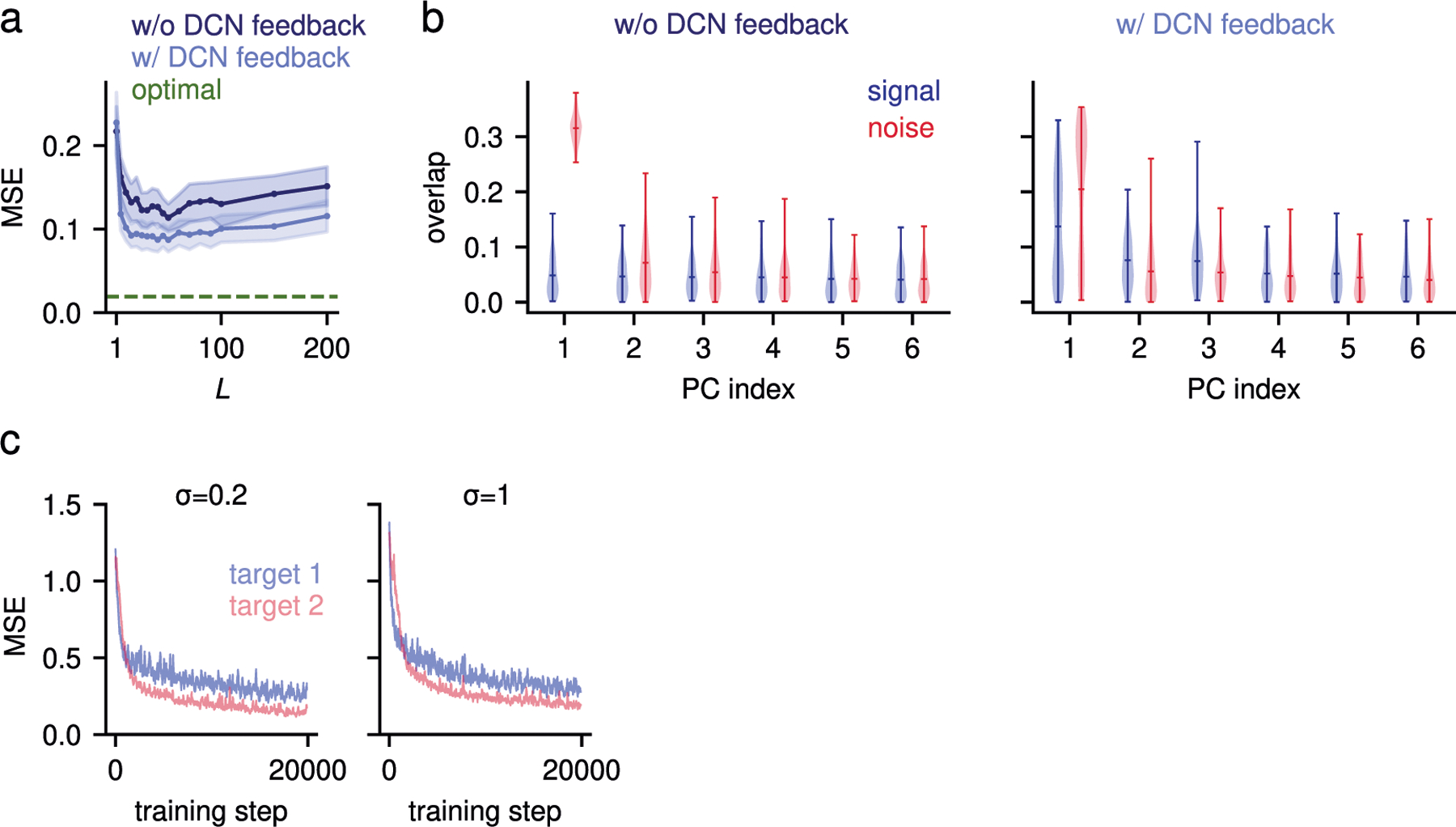
a: Performance on the forward model task is non-monotonic with the pontine in-degree L. We plot the MSE on the forward model task as a function of L for the network with and without feedback from DCN. The best L is of the same order as we found for the classification task in Fig. 6a. We set $\sigma =1$, while all the other parameters are the same as in Fig. 6e. The solid lines and shaded areas indicate the mean and standard deviation of the MSE across network realizations, respectively. b: DCN feedback leads to higher overlap of compression weights with signal principal components. We define the overlap of the weights onto unit $i$ of the compression layer with the $j^{\text{th}}$ PC as overla ${\text{overlap}}_{\text{IJ}}={\sum }_{k=1}^N{G}_{ik}{A}_{kj}$, where G is the compression matrix learned without (left) or with (right) the feedback from DCN, while $A$ is the embedding matrix of the task-relevant components (blue) or task-irrelevant components (red). The violin plot shows the mean and distribution of the overlaps across compression layer units. We set $\sigma =1.8$ and L = 50, while all the other parameters are the same as in Fig. 6e. In the violin plots, the whiskers indicate the entire data range, and the horizontal line indicates the median of the distribution. c: Performance on the forward model task while the compression weights are adjusted using our modified version of Oja’s rule in the presence of feedback from DCN, for two different levels of input noise and two target dimensions. All the other parameters are the same as in Fig. 6e.

Extended Data Fig. 6 |. Dimension and noise contributions to local decorrelation performance.

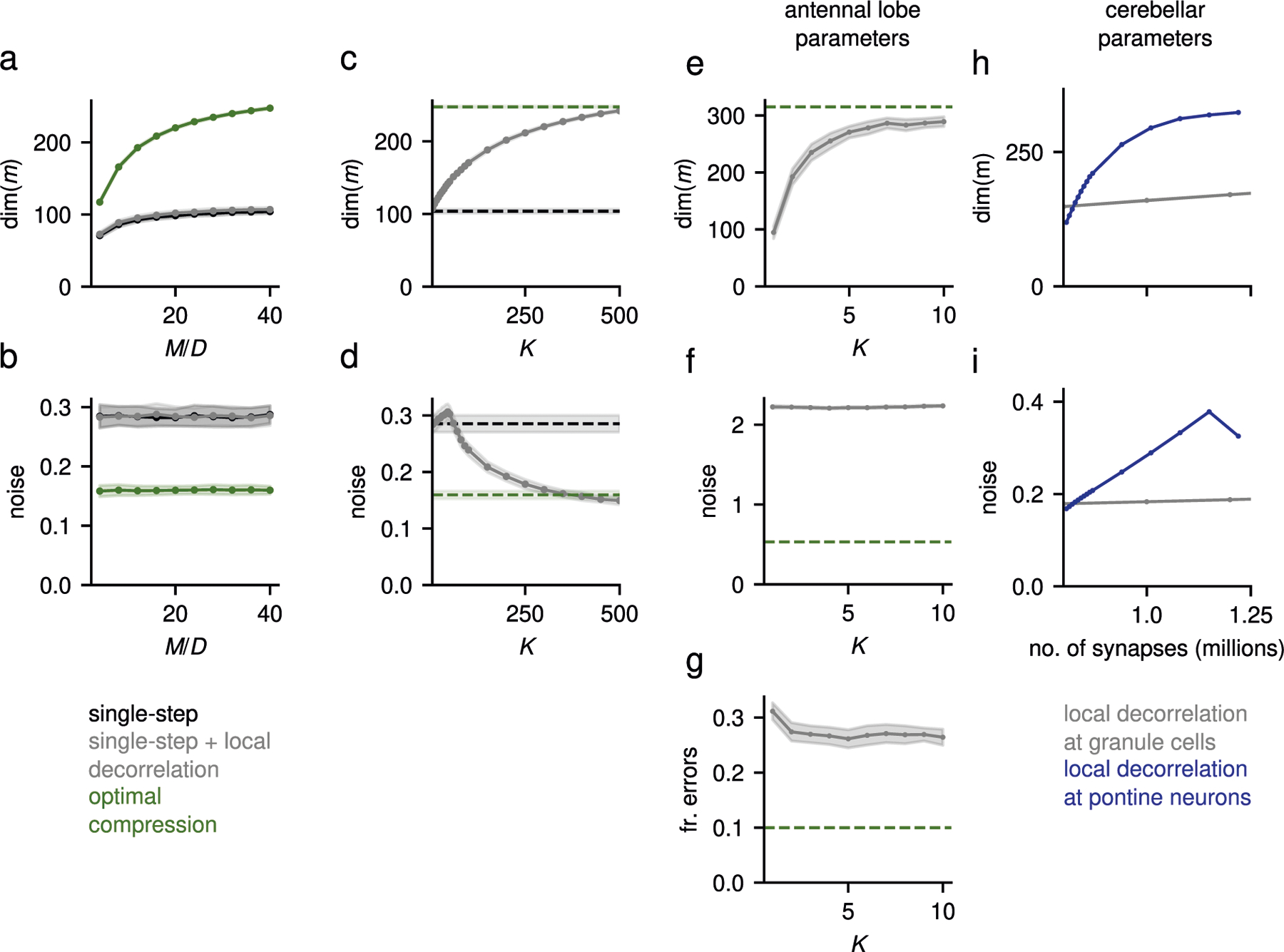
a, b: Dimension (a) and noise (b) contributions to the performance shown in Fig. 8b, using the same parameters. c, d: Dimension (c) and noise (d) contributions to the performance shown in Fig. 8c, using the same parameters. e-g: Dimension (e) and noise (f) contributions to the performance (g), for the antennal lobe architecture, as a function of the in-degree of Kenyon cells $\mathbf{K}$. Input was generated using a clustered representation. The green dashed line indicates the value obtained with optimal compression. The parameters were chosen to be consistent with the insect olfactory system anatomy, that is $\text{D}=\text{Nc}=50,\text{N}=1000,\text{M}=2000,\text{p}=1,\text{f}=0.1,\sigma =1,\text{P}=100$. Note that when K ≥ 8, the local decorrelation strategy requires more synapses than the optimal compression one, for which K = 7 and L = 20. h, i: Dimension (h) and noise (i) contributions to the performance shown in Fig. 8d, using the same parameters. For all panels, the shaded areas indicate the standard deviation across network realizations.

Extended Data Fig. 7 |. Effect of nonlinearities at the compression layer.

To achieve a performance with nonlinear compression layer units comparable to that of linear units, we set Nc = 250. To maximize the dimension of the compression layer after the nonlinearity, we also introduced a random rotation of the optimal compression matrix (see Methods 5). a: Dimension of the compression layer representation for linear versus nonlinear (ReLU) compression. For ReLU compression, the nonlinearity is applied after random (left), PC-aligned (center), and whitening compression (right). b: Same as a, but showing the noise strength at the compression layer ${\Delta }_{\text{c}}$. c: Same as a, but showing the fraction of errors in the random classification task. In panels a-c, the box boundary extends from the first to the third quartile of the data. The whiskers extend from the box by 1.5 times the inter-quartile range. The horizontal line indicates the median. d: Fraction of errors over training when the compression weights are trained using gradient descent and the compression layer units are nonlinear (ReLU). For comparison, the horizontal dashed lines indicate the performance of networks with linear compression layer units. The solid lines indicate the mean over 10 network realizations and the shading indicates the standard deviation across network realizations. e: Performance at convergence for the same networks as in d. For all panels, parameters were N = D = P = 500, N_c = 250, M = 2000, f = 0.1, f_c = 0.3, and $\sigma =0.1$.

Extended Data Fig. 8 |. Expansion layer dimension and noise strength depend on compression layer dimension and noise strength.

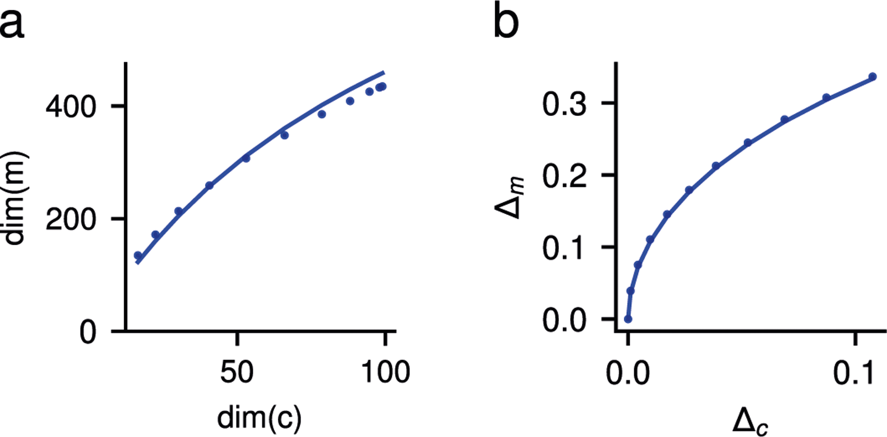
a: Dimension of the expansion layer representation as a function of the compression layer one. The compression layer representation was distributed, and its dimension was varied by changing $p$ between 0 and 1. b: Noise strength ${\Delta }_{\text{m}}$ at the expansion layer as a function of the noise strength at the compression layer. Noise was additive, Gaussian, and isotropic at the compression layer, with standard deviation varying from 0 to 0.1. In both panels, solid lines show the theoretical result and dots are simulation results, averaged over 10 network realizations. Standard deviation of numerical simulations is not visible because it is smaller than the size of the marker. Parameters: N_c = 100, M = 1000, f = 0.1.

Data availability

The data analyzed in this study was previously published in Hallem and Carlson²⁶ and Wagner et al.¹³, and is available upon request.

References

- 1.Yamins DLK & DiCarlo JJ Using goal-driven deep learning models to understand sensory cortex. Nat. Neurosci 19, 356–365 (2016). [DOI] [PubMed] [Google Scholar]
- 2.Bell CC, Han V & Sawtell NB Cerebellum-like structures and their implications for cerebellar function. Annu. Rev. Neurosci 31, 1–24 (2008). [DOI] [PubMed] [Google Scholar]
- 3.Marr D A theory of cerebellar cortex. J. Physiol 202, 437–470 (1969). [DOI] [PMC free article] [PubMed] [Google Scholar]
- 4.Babadi B & Sompolinsky H Sparseness and expansion in sensory representations. Neuron 83, 1213–1226 (2014). [DOI] [PubMed] [Google Scholar]
- 5.Litwin-Kumar A, Harris KD, Axel R, Sompolinsky H & Abbott LF Optimal degrees of synaptic connectivity. Neuron 93, 1153–1164.e7 (2017). [DOI] [PMC free article] [PubMed] [Google Scholar]
- 6.Cayco-Gajic NA & Silver RA Re-evaluating circuit mechanisms underlying pattern separation. Neuron 101, 584–602 (2019). [DOI] [PMC free article] [PubMed] [Google Scholar]
- 7.Brodal P & Bjaalie JG Organization of the pontine nuclei. Neurosci. Res 13, 83–118 (1992). [DOI] [PubMed] [Google Scholar]
- 8.Chen WR & Shepherd GM The olfactory glomerulus: a cortical module with specific functions. J. Neurocytol 34, 353–360 (2005). [DOI] [PubMed] [Google Scholar]
- 9.Bhandawat V, Olsen SR, Gouwens NW, Schlief ML & Wilson RI Sensory processing in the Drosophila antennal lobe increases reliability and separability of ensemble odor representations. Nat. Neurosci 10, 1474–1482 (2007). [DOI] [PMC free article] [PubMed] [Google Scholar]
- 10.Olsen SR & Wilson RI Lateral presynaptic inhibition mediates gain control in an olfactory circuit. Nature 452, 956–960 (2008). [DOI] [PMC free article] [PubMed] [Google Scholar]
- 11.Olsen SR, Bhandawat V & Wilson RI Divisive normalization in olfactory population codes. Neuron 66, 287–299 (2010). [DOI] [PMC free article] [PubMed] [Google Scholar]
- 12.Guo J-Z et al. Disrupting cortico-cerebellar communication impairs dexterity. eLife 10, e65906 (2021). [DOI] [PMC free article] [PubMed] [Google Scholar]
- 13.Wagner MJ et al. Shared cortex-cerebellum dynamics in the execution and learning of a motor task. Cell 177, 669–682. e24 (2019). [DOI] [PMC free article] [PubMed] [Google Scholar]
- 14.Vosshall LB, Wong AM & Axel R An olfactory sensory map in the fly brain. Cell 102, 147–159 (2000). [DOI] [PubMed] [Google Scholar]
- 15.Marin EC, Jefferis GSXE, Komiyama T, Zhu H & Luo L Representation of the glomerular olfactory map in the Drosophila brain. Cell 109, 243–255 (2002). [DOI] [PubMed] [Google Scholar]
- 16.Wong AM, Wang JW & Axel R Spatial representation of the glomerular map in the Drosophila protocerebrum. Cell 109, 229–241 (2002). [DOI] [PubMed] [Google Scholar]
- 17.Berck ME et al. The wiring diagram of a glomerular olfactory system. elife 5, e14859 (2016). [DOI] [PMC free article] [PubMed] [Google Scholar]
- 18.Bates AS et al. Complete connectomic reconstruction of olfactory projection neurons in the fly brain. Curr. Biol 30, 3183–3199.e6 (2020). [DOI] [PMC free article] [PubMed] [Google Scholar]
- 19.Chadderton P, Margrie TW & Häusser M Integration of quanta in cerebellar granule cells during sensory processing. Nature 428, 856–860 (2004). [DOI] [PubMed] [Google Scholar]
- 20.Ito I, Ong RC-Y, Raman B & Stopfer M Sparse odor representation and olfactory learning. Nat. Neurosci 11, 1177–1184 (2008). [DOI] [PMC free article] [PubMed] [Google Scholar]
- 21.Kolkman KE, McElvain LE & du Lac S Diverse precerebellar neurons share similar intrinsic excitability. J. Neurosci 31, 16665–16674 (2011). [DOI] [PMC free article] [PubMed] [Google Scholar]
- 22.Shenoy KV, Sahani M & Churchland MM Cortical control of arm movements: a dynamical systems perspective. Annu. Rev. Neurosci 36, 337–359 (2013). [DOI] [PubMed] [Google Scholar]
- 23.Rumelhart DE, Hinton GE & Williams RJ Learning representations by back-propagating errors. Nature 323, 533–536 (1986). [Google Scholar]
- 24.Caron SJC, Ruta V, Abbott LF & Axel R Random convergence of olfactory inputs in the Drosophila mushroom body. Nature 497, 113–117 (2013). [DOI] [PMC free article] [PubMed] [Google Scholar]
- 25.Gruntman E & Turner GC Integration of the olfactory code across dendritic claws of single mushroom body neurons. Nat. Neurosci 16, 1821–1829 (2013). [DOI] [PMC free article] [PubMed] [Google Scholar]
- 26.Hallem EA & Carlson JR Coding of odors by a receptor repertoire. Cell 125, 143–160 (2006). [DOI] [PubMed] [Google Scholar]
- 27.Friedrich RW & Wiechert MT Neuronal circuits and computations: pattern decorrelation in the olfactory bulb. FEBS Lett. 588, 2504–2513 (2014). [DOI] [PubMed] [Google Scholar]
- 28.Schlegel P et al. Information flow, cell types and stereotypy in a full olfactory connectome. eLife 10, e66018 (2021). [DOI] [PMC free article] [PubMed] [Google Scholar]
- 29.Peters AJ, Lee J, Hedrick NG, O’Neil K & Komiyama T Reorganization of corticospinal output during motor learning. Nat. Neurosci 20, 1133–1141 (2017). [DOI] [PMC free article] [PubMed] [Google Scholar]
- 30.Wolpert DM, Miall RC & Kawato M Internal models in the cerebellum. Trends Cogn. Sci 2, 338–347 (1998). [DOI] [PubMed] [Google Scholar]
- 31.Russo AA et al. Motor cortex embeds muscle-like commands in an untangled population response. Neuron 97, 953–966. e8 (2018). [DOI] [PMC free article] [PubMed] [Google Scholar]
- 32.Saxena S, Russo AA, Cunningham J & Churchland MM Motor cortex activity across movement speeds is predicted by network-level strategies for generating muscle activity. eLife 11, e67620 (2022). [DOI] [PMC free article] [PubMed] [Google Scholar]
- 33.Gallego JA, Perich MG, Chowdhury RH, Solla SA & Miller LE Long-term stability of cortical population dynamics underlying consistent behavior. Nat. Neurosci 23, 260–270 (2020). [DOI] [PMC free article] [PubMed] [Google Scholar]
- 34.Oja E Simplified neuron model as a principal component analyzer. J. Math. Biol 15, 267–273 (1982). [DOI] [PubMed] [Google Scholar]
- 35.Pehlevan C & Chklovskii DB Optimization theory of Hebbian/anti-Hebbian networks for PCA and whitening. In 53rd Annual Allerton Conference on Communication, Control, and Computing, Monticello, IL, USA: 1458–1465 (Allerton, 2015). [Google Scholar]
- 36.Schwarz C & Thier P Binding of signals relevant for action: towards a hypothesis of the functional role of the pontine nuclei. Trends Neurosci. 22, 443–451 (1999). [DOI] [PubMed] [Google Scholar]
- 37.Pehlevan C, Hu T & Chklovskii DB A Hebbian/anti-Hebbian neural network for linear subspace learning: a derivation from multidimensional scaling of streaming data. Neural Comput. 27, 1461–1495 (2015). [DOI] [PubMed] [Google Scholar]
- 38.Barak O, Rigotti M & Fusi S The sparseness of mixed selectivity neurons controls the generalization–discrimination trade-off. J. Neurosci 33, 3844–3856 (2013). [DOI] [PMC free article] [PubMed] [Google Scholar]
- 39.Ganguli S & Sompolinsky H Compressed sensing, sparsity, and dimensionality in neuronal information processing and data analysis. Annu. Rev. Neurosci 35, 485–508 (2012). [DOI] [PubMed] [Google Scholar]
- 40.Barlow HB in Sensory Communication (ed. Rosenblith WA) 216–234 (MIT Press, 1961). [Google Scholar]
- 41.Atick JJ Could information theory provide an ecological theory of sensory processing? Netw. Comput. Neural Syst 3, 213–251 (1992). [DOI] [PubMed] [Google Scholar]
- 42.Simoncelli EP Vision and the statistics of the visual environment. Curr. Opin. Neurobiol 13, 144–149 (2003). [DOI] [PubMed] [Google Scholar]
- 43.Kramer MA Nonlinear principal component analysis using autoassociative neural networks. AlChE J. 37, 233–243 (1991). [Google Scholar]
- 44.Benna MK & Fusi S Place cells may simply be memory cells: memory compression leads to spatial tuning and history dependence. Proc. Natl Acad. Sci. USA 118, e2018422118 (2021). [DOI] [PMC free article] [PubMed] [Google Scholar]
- 45.Baldi P & Hornik K Neural networks and principal component analysis: learning from examples without local minima. Neural Netw. 2, 53–58 (1989). [Google Scholar]
- 46.Apps R & Garwicz M Anatomical and physiological foundations of cerebellar information processing. Nat. Rev. Neurosci 6, 297–311 (2005). [DOI] [PubMed] [Google Scholar]
- 47.Oscarsson O Functional organization of the spino- and cuneocerebellar tracts. Physiol. Rev 45, 495–522 (1965). [DOI] [PubMed] [Google Scholar]
- 48.Kennedy A et al. A temporal basis for predicting the sensory consequences of motor commands in an electric fish. Nat. Neurosci 17, 416–422 (2014). [DOI] [PMC free article] [PubMed] [Google Scholar]
- 49.Bratton B & Bastian J Descending control of electroreception. II. Properties of nucleus praeeminentialis neurons projecting directly to the electrosensory lateral line lobe. J. Neurosci 10, 1241–1253 (1990). [DOI] [PMC free article] [PubMed] [Google Scholar]
- 50.Kazama H & Wilson RI Origins of correlated activity in an olfactory circuit. Nat. Neurosci 12, 1136–1144 (2009). [DOI] [PMC free article] [PubMed] [Google Scholar]
- 51.Chapochnikov NM, Pehlevan C & Chklovskii DB Normative and mechanistic model of an adaptive circuit for efficient encoding and feature extraction. Proc. Natl Acad. Sci. USA 120, e21174841 (2023). [DOI] [PMC free article] [PubMed] [Google Scholar]
- 52.Kebschull JM et al. Cerebellar nuclei evolved by repeatedly duplicating a conserved cell-type set. Science 370, eabd5059 (2020). [DOI] [PMC free article] [PubMed] [Google Scholar]
- 53.Barbosa J, Proville R, Rodgers CC, Ostojic S & Boubenec Y Flexible selection of task-relevant features through across-area population gating. Preprint at bioRxiv 10.1101/2022.07.21.500962 (2022). [DOI] [PMC free article] [PubMed] [Google Scholar]
- 54.Leergaard TB & Bjaalie JG Topography of the complete corticopontine projection: from experiments to principal Maps. Front. Neurosci 1, 211–223 (2007). [DOI] [PMC free article] [PubMed] [Google Scholar]
- 55.Kratochwil CF, Maheshwari U & Rijli FM The long journey of pontine nuclei neurons: from rhombic lip to cortico-ponto-cerebellar circuitry. Front. Neural Circuits 10.3389/fncir.2017.00033 (2017). [DOI] [PMC free article] [PubMed] [Google Scholar]
- 56.Mihailoff GA, Lee H, Watt CB & Yates R Projections to the basilar pontine nuclei from face sensory and motor regions of the cerebral cortex in the rat. J. Comp. Neurol 237, 251–263 (1985). [DOI] [PubMed] [Google Scholar]
- 57.Lanore F, Cayco-Gajic NA, Gurnani H, Coyle D & Silver RA Cerebellar granule cell axons support high-dimensional representations. Nat. Neurosci 24, 1142–1150 (2021). [DOI] [PMC free article] [PubMed] [Google Scholar]
- 58.Xie M, Muscinelli S, Harris KD & Litwin-Kumar A Task-dependent optimal representations for cerebellar learning. Preprint at bioRxiv 10.1101/2022.08.15.504040 (2022). [DOI] [PMC free article] [PubMed] [Google Scholar]
- 59.Stewart GW The efficient generation of random orthogonal matrices with an application to condition estimators. SIAM J. Numer. Anal 17, 403–409 (1980). [Google Scholar]
- 60.Abbott LF, Rajan K & Sompolinsky H The Dynamic Brain: An Exploration of Neuronal Variability and its Functional Significance (eds Ding M & Glanzman D) 65–82 (Oxford Academic, 2011). [Google Scholar]
- 61.Kingma DP & Ba J Adam: a method for stochastic optimization. Preprint at arXiv 10.48550/arXiv.1412.6980 (2017). [DOI] [Google Scholar]
- 62.Fagg A, Sitkoff N, Barto A & Houk J Cerebellar learning for control of a two-link arm in muscle space. In Proc. of International Conference on Robotics and Automation, Albuquerque, NM, USA, Vol. 3, 2638–2644 (IEEE, 1997). [Google Scholar]
Associated Data
This section collects any data citations, data availability statements, or supplementary materials included in this article.
Supplementary Materials
Data Availability Statement