The benthic food web connects the estuarine habitat mosaic to adjacent ecosystems

Abstract

Energy flows from land to sea and between pelagic and benthic environments have the potential to increase the connectivity between estuaries and adjacent ecosystems as well as among estuarine habitats. To identify such energy flows and the main trophic pathways of energy transfer in the Minho River estuary, we investigated the spatial and temporal fluctuations of carbon and nitrogen stable isotope ratios in benthic (and their potential food sources) and epibenthic consumers. Sampling was conducted along the estuarine salinity gradient from winter to summer of 2011. We found that the carbon (δ¹³C = ¹³C/¹²C) and nitrogen (δ¹⁵N = ¹⁵N/¹⁴N) stable isotope ratios of the most abundant benthic and epibenthic consumers varied along the salinity gradient. The δ¹³C values increased seaward, whereas the opposite pattern was found for the δ¹⁵N, especially during the summer. The stable isotope ratios revealed two trophic pathways in the Minho estuary food web. The first pathway is supported by phytoplankton and represented by filter feeders such as zooplankton and some deposit feeders, particularly amphipods and polychaetes. The second pathway is supported by detritus and composed essentially of deposit feeders, which by being consumed, allow detritus to be incorporated into higher trophic levels. Spatial and temporal feeding variations in the estuarine benthic food web are driven by hydrology and proximity to adjacent ecosystems (terrestrial, marine). During high river discharge periods, the δ¹³C_POC (ca. −28‰) and C: N_POM (>10) values suggested an increase of terrestrial-derived OM to the particulate OM pool, which was then used by suspension feeders. During low river discharge periods, marine intrusion increased upriver, which was reflected in benthic consumers’ ¹³C-enriched stable isotope values. No relationship was found between food quality (phytoplankton vs. detritus) and food chain length because the lowest and highest values were associated with freshwater and saltmarsh areas, respectively, both dominated by the detrital pathway. This study demonstrates that benthic consumers enhance the connectivity between estuaries and its adjacent ecosystems by utilizing subsidies of terrestrial and marine origin and that benthic-pelagic coupling is an important energy transfer mechanism to the benthic food web.

1. Introduction

Estuaries are among the most productive ecosystems on the planet and produce highly variable food webs associated with different habitats and distinct sources of organic matter (OM) (Canuel et al., 1995; Selleslagh et al., 2015). At the landscape scale, estuarine habitats are interconnected by several processes and events which allow the movements of nutrients, detritus, and organisms between habitats and across ecosystem boundaries (Vanni et al., 2004; Sheaves, 2009). The cross-habitat movements of OM create a land to sea gradient; generally, the contribution of terrestrial-derived OM to estuaries decreases towards the ocean, and the contribution of marine-derived OM follows the opposite pattern (Antonio et al., 2012; Valiela and Bartholomew, 2015; Dias et al., 2016). The magnitude of these movements varies temporally: daily with tides, seasonally with river inflow, and annually with different climatic patterns (Riley et al., 2004; Hoffman and Bronk, 2006; Dias et al., 2016). Animal movements are also an important source of cross-ecosystem subsidies (e.g., Howe and Simenstad, 2015). That is, animals feed and grow in one ecosystem and afterward move to another ecosystem where they support local food webs as prey or by translocating nutrients via death and decay, as exemplified by the anadromous species that subsidize freshwater ecosystems with marine-derived nutrients (Schindler et al., 2003; Kohler et al., 2012; Weaver et al., 2016). Thus, the cross-ecosystem transport of OM can provide energy subsidies to spatially disparate communities (e.g., Polis et al., 1997; Antonio et al., 2012; Hoffman et al., 2015).

Secondary production and food web complexity depend on the quality and quantity of the basal OM sources (Rooney and McCann, 2011). Pelagic pathways, associated with phytoplankton consumption, are considered more efficient than benthic pathways associated with the consumption of detritus because this is a less labile OM source (Rooney and McCann, 2011). Nonetheless, a diverse array of OM sources, including terrestrial-derived OM (Kasai and Nakata, 2005; Dias et al., 2014), phytoplankton (Yokoyama et al., 2005), benthic microalgae (Kang et al., 2003), and coastal algae (Currin et al., 1995), support benthic communities. Thus, benthic productivity depends partially on the quality and quantity of OM transferred from the pelagic to the benthic habitats via sedimentation, which can increase the incorporation of allochthonous OM (i.e., external inputs) into the food web (Hughes et al., 2000; Bergamino and Richoux, 2015), potentially increasing estuarine secondary production and food web stability (Huxel and McCann, 1998; Carpenter et al., 2005).

Benthic organisms generally are opportunistic feeders, and their diet is spatially influenced by differences in the primary OM sources available (Keats et al., 2004) and feeding habits (Lucero et al., 2006). Thus, different trophic pathways may arise in estuarine benthic food webs due to the variability of both trophic guild diversity and resources available, which tend to be higher in mixing areas such as estuaries (Hoffman et al., 2015). Consequently, benthic organisms influence the spatial patterns of trophic relationships in estuarine food webs. However, due to their generally low body size and high variability in the available OM sources, which includes detritus of different origins (e.g., aquatic and terrestrial plants, senescent phytoplankton), it is challenging to determine feeding relationships using stomach content analysis. Alternatively, carbon (δ¹³C = ¹³C/¹²C) and nitrogen (δ¹⁵N = ¹⁵N/¹⁴N) stable isotope ratios provide time-integrated information about both trophic levels and energy flow through food webs. The δ¹⁵N value of an organism is typically enriched by ca. 3‰ relative to its diet and is used to determine the trophic position of an organism (Minagawa and Wada, 1984; Vander Zanden and Rasmussen, 2001). The δ¹³C value changes little (ca. 1‰ per trophic level) as carbon moves through the food web and is used to evaluate the sources of energy used by an organism (Peterson and Fry, 1987; Vander Zanden and Rasmussen, 2001).

Benthic organisms have limited mobility and therefore are excellent models for studying the importance of energy pathways in different locations within an estuary. We hypothesize that benthic consumers from different areas within the estuary will have distinct stable isotope ratios along the spatial gradient owing to differential food availability and connectivity with other ecosystems (Antonio et al., 2012; Dias et al., 2016). We also hypothesize that consumer diets shift through time due to seasonal variability in local primary production and detrital inputs due to river discharge. During high river discharge periods, riverine and terrestrial OM inputs to the estuary can increase, augmenting terrestrial-derived OM utilization by aquatic consumers (Hoffman et al., 2008). During low river discharge periods, the residence time is elongated, allowing estuarine phytoplankton biomass to accumulate, thus increasing the availability of this high-quality food source to estuarine consumers (Hoffman and Bronk, 2006; Dias et al., 2016). In this study, we used stable isotopes to examine the benthic food webs in five stations located along the salinity gradient of an estuary of the NW-Iberian Peninsula, over three seasons with variable river discharge conditions to identify the OM sources assimilated by benthic and zooplankton organisms according to their availability. Additionally, we determined the food chain length in the estuarine benthic food web based on the spatial and temporal variability of N stable isotope ratios of the most abundant epibenthic consumers.

2. Methods

2.1. Study area

This study was conducted in the shallow Minho River, located in the NW-Iberian Peninsula (Europe; Fig. 1). Its watershed is 17,080 km², of which 95% is located in Spain and 5% in Portugal. The river is 343 km long; 76 km serves as the northwestern Portuguese-Spanish border (Antunes et al., 2011). The annual average river discharge is 300 m³ s⁻¹ (Ferreira et al., 2003); it can vary between 100 m³ s⁻¹ during summer, and over 600 m³ s⁻¹ during winter (Confederación Hidrográfica del Miño-Sil, 2018 in Dias et al., 2019b; Fig. 2). The limit of tidal influence is about 40 km inland, and the uppermost 30 km are tidal freshwater wetlands (TFW; Vilas and Somoza, 1984). The estuary has an area of 23 km², 9% of which are intertidal areas. The estuary is mesotidal, with tides ranging between 0.7 m and 3.7 m (Alves, 1996).

Fig. 1.

Location of the sampling stations along the Minho River estuary.

Fig. 2.

Surface and bottom salinity values, and mean properties of the particulate organic matter [POM: including δ¹⁵N, δ¹³C, molar C:N, and chlorophyll a (Chl a) concentration (μg L⁻¹)] in 5 stations along the Minho River estuarine mixing gradient, between January and September 2011.

Typically, the estuary has low chlorophyll a (Chl a) concentrations: from 1.3 μg L⁻¹ in low salinity areas to 2.1 μg L⁻¹ in brackish areas (average values from 2000 to 2010; Brito et al., 2012). The abundance and distribution of subtidal macrozoobenthos and epibenthos in the Minho River estuary are influenced by salinity (Sousa et al., 2008; Costa-Dias et al., 2010), and by the sediment granulometry and organic matter content in the case of macrozoobenthos (Sousa et al., 2008). At the river mouth, salinity varies between 25 in winter and 32 in summer during high tide, and it reaches 0 at low tide during periods of higher river discharge. The sediment is sandy and has low organic matter content, despite being often covered by debris from upriver. The dominant macrozoobenthos are the polychaete Hediste diversicolor and the amphipod Hautorius arenarius (Sousa et al., 2008). In the adjacent saltmarsh, sediment granulometry is smaller, and the organic matter content is higher than at the river mouth. Here, the dominant species are H. diversicolor, the isopod Cyathura carinata, and the bivalve Scrobicularia plana (Sousa et al., 2008). In the middle estuary, salinity fluctuates between 0 in winter and 20 during summer, and the dominant macrozoobenthos are the amphipods Corophium multisetosum and Gammarus chevreuxi, and the invasive bivalve Corbicula fluminea (Sousa et al., 2008). The dominant epibenthic species present from the river mouth to the middle estuary are the crustaceans Crangon crangon and Carcinus maenas, and the teleost Pomatoschistus microps (Souza et al., 2013). In the tidal freshwater (TFW) area, the substrate is sandy and often covered by aquatic vegetation (e.g., Elodea canadensis, Egerea sp.), and C. fluminea represents >90% of the total benthic macrofauna biomass (Sousa et al., 2005, 2008). The epibenthic community in the TFW is dominated by the freshwater shrimp Atyaephyra desmaresti and by the epibenthic teleosts Cobitis paludica and Platichthys flesus (Costa-Dias et al., 2010).

2.2. Field sampling

Sampling was conducted during full-moon spring tides, from January to September 2011, and at five stations along the salinity gradient: 1- adjacent to the river mouth; 2- at the Coura river saltmarsh, located at ~4 km from the river mouth; 3–8 km upstream from the river mouth in the salinity transition zone; 4 and 5- located in the TFW area at 15 km and 21 km, from the river mouth, respectively (Fig. 1).

At each station, surface (50–100 cm below the surface) and bottom water samples (0.5 m off the bottom) were collected using a 2-L Ruttner bottle to determine the concentration of chlorophyll a (Chl a: μg L⁻¹), the isotopic composition of POM (including particulate organic carbon (POC) δ¹³C, particulate nitrogen (PN) δ¹⁵N, and molar C:N). Salinity was measured with a YSI model 6820 QS probe and reported using the Practical Salinity Scale. The POM and Chl a water samples (POM: 1 L, Chl a: 0.5 L) were pre-filtered with a 150 μm sieve and filtered onto a pre-combusted (500 °C for 2 h) Whatman GF/F and Whatman GF/C filters, respectively, which were stored frozen (−20 °C).

Microphytobenthos (MPB) samples were collected by scraping artificial substrates deployed in the sediment at least once a month, which were left at each site during the entire study. Macroalgae were collected in stations 1 to 3, and vascular plants in stations 2, 4, and 5.

Zooplankton samples were collected from surface waters using a plankton net (200 μm mesh) and immediately preserved in 70% ethanol. Macrozoobenthos were sampled using a Van Veen grab. Epibenthic organisms (i.e., C. crangon, C. maenas, Gasterosteus aculeatus, P. microps, P. flesus) were sampled in January, March, April, July–September 2011 using a 1-m beam trawl (5 mm stretched mesh) towed at 2 km h⁻¹. Macrozoobenthos and epibenthos samples were stored frozen (−20 °C).

2.3. Laboratory analyses

Filter samples used for Chl a analysis were submerged in 90% acetone to extract the pigments and then analyzed on a Spectronic 20 Genesys spectrophotometer. Chlorophyll a concentration was calculated following Lorenzen (1967).

Filters used for POM and MPB analyses were fumigated with concentrated HCl to remove inorganic carbonates, rinsed with deionized water, placed in a sterile Petri dish, and dried at 60 °C for 24 h; this procedure is expected to produce only slight changes, ca. 0.4‰, in δ¹⁵N values (Lorrain et al., 2003). Macroalgae and vascular plants were cleaned with deionized water to remove epiphytes, dried at 60 °C, and ground to a fine powder with a mixer mill for stable isotope analyses.

All the consumers were sorted, identified, measured when applicable, dried in an oven at 60 °C, and ground to a fine homogeneous powder. The macrozoobenthos samples consisted of whole individuals, except for bivalves, where we used the foot muscle for stable isotopes analyses, while for epibenthic crustaceans and fish, we used muscle tissue.

Stable isotope ratios were measured using a Thermo Scientific Delta V Advantage IRMS via a Conflo IV interface (Marinnova, University of Porto). We report stable isotope ratios in δ notation, δX = (R_sample/R_standard – 1) x 10³, where X is the C or N stable isotope, R is the ratio of heavy:light stable isotopes. The δ¹³C and δ¹⁵N are expressed in units per mill (‰) relative to Vienna Pee Dee Belemnite and air, respectively. The analytical error, the mean SD of replicate reference material, was ±0.1 ‰ for both δ¹³C and δ¹⁵N. The C:N values for sources and consumers were derived from the stable isotope analysis.

2.4. Data analysis

We used carbon (C) and nitrogen (N) stable isotope ratio bi-plots to identify the sources of OM to the estuarine benthic consumers and zooplankton. The C and N stable isotope ratios of POM, MPB, emerged aquatic vegetation (EAV), submerged aquatic vegetation (SAV), and terrestrial plants were measured in this study. The C and N stable isotope ratios for phytoplankton, sediment organic matter (SOM), and C4 saltmarsh plants were compiled from previous studies conducted in this ecosystem (freshwater and estuarine phytoplankton, and SOM; Dias et al., 2014, 2016), and from the literature (marine phytoplankton and C4 saltmarsh plants: Fry and Sherr, 1984; Deegan and Garritt, 1997; Bode et al., 2007; McMahon et al., 2013). Standard deviation (±SD) will be used as a measure of data dispersion when reporting mean values.

To quantify OM source contributions to each station’s most frequently sampled benthic species, we used a dual-stable isotope mixing model that uses Bayesian inference to solve indeterminate linear mixing equations (i.e., two stable isotope ratios and more than three diet sources). Indeterminate linear mixing equations produce a probability distribution representing a given source’s likelihood to contribute to the consumer (Parnell et al., 2010). We used the model Stable Isotope Analysis in R (SIAR), which allows each of the sources and the trophic enrichment factor (TEF; or trophic fractionation) to be assigned a normal distribution (Parnell et al., 2010). SIAR produces the distribution of feasible solutions to the mixing problem and estimates credibility intervals (95% CI in this study), which are analogous to the confidence intervals used in frequentist statistics. SIAR also includes a residual error term. In the SIAR mixing model, we adjusted the δ¹³C and δ¹⁵N values for one or two trophic levels using the TEF estimates from Vander Zanden and Rasmussen (2001): −0.41‰ or + 0.5‰ δ¹³C (−0.41‰ for primary consumers and + 0.5‰ for secondary consumers), and + 2.5‰ or + 5.9‰ δ¹⁵N (+2.5‰ for primary consumers and + 3.4‰ for secondary consumers). For modeling purposes, months were grouped according to season (Winter: January–March; Spring: April–June; Summer: July–September), and stations 4 and 5 were grouped as TFW due to low and stable salinity values throughout the year. In the Minho River, typically, river discharge is relatively high during winter, decreasing during spring (intermediate conditions), and reaching the lowest values during summer (Dias et al., 2016). We anticipate that the river discharge effect on marine intrusion would cause consumers from the low-salinity portion of the estuary to undergo an isotopic composition shift from relatively ¹³C- and ¹⁵N-depleted (high discharge, strong freshwater influence) to ¹³C- and ¹⁵N-enriched (low discharge, strong marine influence).

To establish general comparisons between the stable isotopes and mixing model results among trophic guild groups, consumers were grouped as follow: filter-feeding (FF; zooplankton and bivalves; Kleppel, 1993; Verdelhos et al., 2005; Atkinson et al., 2011), deposit feeders (DF; gastropods, insect larvae, amphipods, isopods, Atyaephyra desmarestii; Gerdol and Hughes, 1994; Bode et al., 2006; Lucero et al., 2006; Pestana et al., 2007), epibenthic omnivores (EO; Carcinus maenas, Crangon crangon; Pihl, 1985), and zoobenthivores (EZB; Gasterosteus aculeatus, Pomatoschistus microps, Platichthys flesus, Solea solea; Pihl, 1985; Jackson et al., 2004).

The trophic position (TP) was calculated following Post (2002a): TP = λ + (δ¹⁵N_consumer – δ¹⁵N_baseline)/3.4, where λ represents the trophic level of the baseline organism, δ¹⁵N_consumer is the stable isotope value of the consumer, δ¹⁵N_baseline is the stable isotope value of the baseline organism, 3.4 indicates the trophic fractionation of δ¹⁵N per trophic level for secondary and tertiary consumers (Vander Zanden and Rasmussen, 2001). In this study, copepods were chosen as the baseline organisms because they can assimilate phytoplankton (in the water column and MPB) and OM from the detrital food web (this study); λ was attributed as trophic level 2. To test for differences in TP values a non-parametric factorial ANOVA was used with two factors: season (three levels), station (four levels), and its interaction. For that, we used the function art. con available in the package ARTool (Kay et al., 2021). The effect of size in TP according to species was assessed with the Spearman correlation.

Consumer δ¹³C values were corrected for lipid content because lipids are depleted in ¹³C compared to protein and carbohydrates (DeNiro and Epstein, 1977). Variability in lipid content can bias bulk tissue δ¹³C values and thereby cause dietary or habitat shifts to be incorrectly interpreted. We corrected zooplankton tissue data using the mass balance correction model proposed for zooplankton by Smyntek et al. (2007; Eq. 5). For benthic and epibenthic consumers, we used the mass balance correction for fish muscle tissue proposed by Hoffman and Sutton (2010; Eq. 6), which uses estimates of C:N_protein and Δδ¹³C_lipid that are similar to those from the muscle tissue found for other fish (e.g., Sweeting et al., 2006) and taxonomic groups (e.g., shrimp and zooplankton; Fry et al., 2003; Smyntek et al., 2007). Zooplankton stable isotope ratios were also corrected for ethanol preservation (+0.4‰ δ¹³C, +0.6‰ δ¹⁵N) (Feuchtmayer and Grey, 2003).

All the analyses were performed using the software R, version 4.0.2 (R Core Team, 2020).

3. Results

3.1. Stable isotopic composition of estuarine food web components

The isotopic composition of primary producers collected during this study varied markedly along the salinity gradient in the Minho River estuary (Table 1 and Fig. 2). Stations (S) 1 and 2 were marine to brackish, with salinity varying between 23.1 ± 11.3 (S1) and 20.5 ± 12.4 (S2), S3 represents a brackish water environment (5.4 ± 8.2), owing to daily marine water intrusion and its central position in the estuary, and S4 and S5 are freshwater stations since salinity was always lower than 0.5 (Fig. 2). The average δ¹³C values of POM and MPB collected along the entire gradient increased towards the river mouth, while the average δ¹⁵N values followed the opposite pattern (Table 1 and Fig. 2). Average δ¹⁵N values ranged from 3.1 ± 4.9‰ (terrestrial plants in TFW) to 11.0 ± 2.7‰ (SAV- submerged aquatic vegetation, in TFW), and average δ¹³C values ranged from −28.7 ± 0.3‰ (EAV-emergent aquatic vegetation, TFW) to −15.9 ± 2.3‰ (macroalgae in S1) (Table 1).

Table 1.

Average (± SD) δ¹⁵N and δ¹³C values (‰) of the organic matter (OM) sources collected along the salinity gradient of the Minho River estuary, between January and September 2011. The OM sources include Macroalgae, particulate OM (POM), microphytobenthos (MPB), emergent aquatic vegetation (EAV), submerged aquatic vegetation (SAV), and Terrestrial plants.

	Station 1		Station 2		Station 3		Stations TFW
Sources	δ15N (SD)	δ13C (SD)	δ15N (SD)	δ13C (SD)	δ15N (SD)	δ13C (SD)	δ15N (SD)	δ13C (SD)
Macroalgae	8.5 (0.5)	−13.9 (0.0)	7.7 (2.0)	−17.0 (0.8)	9.3 (1.2)	−12.6 (1.8)
POM	5.0 (3.0)	−22.9 (2.6)	5.4 (1.9)	−24.2 (2.0)	5.5 (1.9)	−25.9 (2.0)	6.4 (1.6)	−28.0 (1.0)
MPB	4.7 (1.9)	−18.0 (1.5)	8.3 (0.9)	−18.6 (1.7)	7.4 (1.9)	−21.3 (3.9)	8.4 (1.7)	−26.4 (2.4)
EAV							5.4 (1.6)	−28.7 (0.3)
SAV							11.0 (2.7)	−21.3 (1.3)
Terrestrial							3.1 (4.9)	−28.2 (1.3)

The quality of the POM pool, as indicated by C:N_POM, was similar between stations and varied between 8.6 ± 2.2 (S3) and 9.8 ± 1.7 (S4), with the highest values observed during high river discharge conditions and across the estuary (Fig. 2). The C:N_POM ≥ 10 in TFW indicates that terrestrial-derived OM contributed substantially to the POM pool in this estuary portion (Hedges et al., 1986, 1997). In the brackish portion of the estuary (S1-S3), average C:N_POM varied between 8 and 9 (Fig. 2), intermediate between terrestrial-derived OM (>10) and marine phytoplankton (~7) (Hedges et al., 1986,1997), indicating that brackish POM was a mixture of riverine POM and marine or estuarine phytoplankton (or both).

Overall, consumers were ¹³C-enriched and ¹⁵N-depleted towards the river mouth (Table 2). Among trophic guilds, filter-feeding (FF) consumers’ average δ¹³C values varied between −32.0‰ in S3 and TFW (zooplankton) and – 16.7 ± 0.60‰ in S1 (Scrobicularia plana), while average deposit feeders (DF) δ¹³C values varied between −29.2‰ in TFW (gastropods) and – 13.9 ± 0.68‰ in S2 (Cyathura carinata) (Table 2). Epibenthic omnivores (EO) average δ¹³C values varied between −19.9 ± 1.84‰ (C. crangon in S3) and – 15.7 ± 0.59‰ (C. crangon in S2), while zoobenthivores (EZB) average δ¹³C values varied between- 25.6 ± 0.10‰ (P. flesus in TFW) and – 17.6 ± 0.89‰ (P. microps in S2) (Table 2).

Table 2.

Carbon and nitrogen stable isotope values (‰, average ± SD), trophic guilds (FF: filter feeders, DF: deposit feeders, EO: epibenthic omnivores, EZB: epibenthic zoobenthivores), and number of replicates (n) of the most abundant benthic and epibenthic consumers in stations (S) 1, 2, 3, and tidal freshwater (TFW) during the winter, spring, and summer of 2011 in the Minho River estuary.

		Winter			Spring			Summer
Consumers	TG	δ13C (SD)	δ15N (SD)	n	δ13C (SD)	δ15N (SD)	n	δ13C (SD)	δ15N (SD)	n
S1
Zooplankton*	FF	−18.7 (0.30)	8.1 (0.25)	4	−19.0 (0.22)	8.2 (0.32)	6	−16.9 (0.44)	6.9 (0.49)	12
Scrobicularia plana	FF	–	–	–	−19.6 (0.10)	6.4 (0.10)	3	−16.7 (0.60)	9.1 (1.40)	12
Hediste diversicolor *	DF	−20.3 (0.30)	9.5 (0.20)	6	−20.5 (1.17)	9.4 (0.33)	4	−19.6 (0.45)	9.3 (0.57)	9
Cyathura carinata *	DF	−15.8 (0.48)	11.2 (0.62)	4	–	–	–	−14.8 (1.21)	10.5 (1.25)	3
Crangon crangon	EO	−18.1 (2.0)	11.9 (1.39)	3	−17.5 (0.80)	10.8 (0.69)	10	−15.9 (0.77)	12.3 (0.43)	11
Carcinus maenas	EO	−19.2 (2.23)	12.7 (1.10)	8	−18.2 (1.00)	12.9 (0.31)	6	−18.5 (0.10)	10.6 (0.10)	3
Pomatoschistus microps	EZB	–	–	–	−19.0 (0.51)	13.3 (0.69)	7	−19.0 (1.37)	12.8 (1.24)	18
Platichthys flesus	EZB	–	–	–	−20.7 (2.74)	13.4 (0.26)	3	−20.5 (1.60)	11.9 (0.64)	3
Solea solea	EZB	–	–	–	−19.0 (1.07)	11.0 (0.39)	11	−18.5 (0.68)	11.7 (0.11)	3
S2
Zooplankton*	FF	−18.6 (0.26)	8.3 (0.21)	6	−18.5 (0.40)	7.1 (0.10)	3	−16.7 (0.98)	7.0 (0.57)	12
Hediste diversicolor *	DF	−20.2 (0.40)	10.7 (0.54)	4	−21.3 (1.00)	11.6 (0.71)	4	−18.0 (0.81)	10.4 (0.55)	6
Cyathura carinata *	DF	−15.0 (0.61)	12.0 (0.54)	6	−15.6 (0.50)	12.7 (0.30)	4	−13.9 (0.68)	11.7 (0.23)	8
Crangon crangon	EO	−17.8 (0.87)	13.2 (0.54)	23	−17.7 (0.99)	12.3 (0.99)	7	−15.7 (0.59)	12.3 (0.43)	33
Carcinus maenas	EO	−19.2 (1.04)	13.2 (0.93)	13	−19.5 (1.50)	13.1 (0.54)	7	−19.5 (0.98)	13.5 (0.80)	17
Pomatoschistus microps	EZB	−18.0 (0.93)	15.1 (0.51)	22	−19.2 (1.45)	14.4 (0.75)	5	−17.6 (0.89)	14.4 (0.45)	16
Platichthys flesus	EZB	–	–	–	−20.7 (0.10)	14.4 (0.10)	2	−19.6 (1.72)	13.6 (0.34)	8
Solea solea	EZB	–	–	–	−19.1 (0.10)	10.8 (0.10)	2	−18.5 (1.49)	11.8 (0.05)	2
S3
Zooplankton*	FF	−32.0	6.5	1	−26.2 (0.10)	8.8 (0.10)	3	−19.1 (2.64)	8.0 (1.14)	10
Corbicula fluminea	FF	−25.3 (0.63)	10.0 (1.08)	35	−26.5 (0.60)	10.5 (0.89)	7	−26.8 (1.57)	11.4 (0.43)	16
Corophium sp.*	DF	−26.4 (1.92)	7.7 (1.74)	7	−23.1 (1.18)	9.4 (0.55)	7	−18.3 (1.51)	9.0 (0.23)	4
Hediste diversicolor *	DF	−28.8 (1.75)	10.0 (0.56)	4	−20.1	10.3	1	−17.8 (1.80)	11.4 (0.79)	6
Cyathura carinata *	DF	−20.8 (0.37)	11.7 (0.75)	6	−20.6 (1.80)	12.0 (0.24)	3	−18.6 (0.29)	12.2 (0.24)	6
Crangon crangon	EO	−17.6 (0.91)	13.5 (0.34)	4	−19.9 (1.84)	12.4 (0.44)	8	−19.1 (1.73)	12.4 (1.10)	27
Carcinus maenas	EO	–	–	–	−17.7 (0.10)	13.1 (0.10)	2	−19.8 (0.57)	13.7 (0.79)	4
Pomatoschistus microps	EZB	−22.5 (0.89)	14.8 (0.26)	10	−21.3 (1.35)	14.0 (0.27)	6	−21.5 (1.33)	14.4 (0.85)	23
Platichthys flesus	EZB	−23.7 (1.56)	12.8 (0.91)	22	−23.9 (1.64)	13.7 (1.07)	5	−21.8 (0.67)	12.6 (0.65)	4
TFW
Zooplankton*	FF	−31.5 (2.21)	11.3 (0.84)	3	−26.9 (3.0)	10.7 (1.18)	3	−27.9 (1.96)	11.4 (0.93)	15
Corbicula fluminea	FF	−26.7 (0.75)	8.3 (0.95)	32	−27.7 (0.98)	8.5 (0.28)	17	−27.4 (1.11)	9.0 (0.67)	20
Corophium sp.*	DF	−25.2 (0.09)	9.5 (0.08)	3	–	–	–	−26.3 (0.27)	10.3 (0.26)	7
Diptera larvae*	DF	−24.7 (2.81)	10.6 (3.34)	4	−25.9 (1.02)	10.3 (0.91)	3	−20.0 (0.58)	11.8 (0.40)	3
Oligochaeta*	DF	−25.0 (0.43)	7.6 (0.45)	6	−24.4 (0.04)	8.0 (0.51)	2	−25.6 (1.08)	8.8 (0.34)	3
Gastropoda*	DF	−29.2	12.2	1	−23.8 (0.15)	10.9 (0.33)	3	−22.7 (1.45)	10.7 (0.61)	5
Atyaephyra desmarestii	DF	−25.2 (1.32)	11.2 (0.67)	36	−24.9 (0.75)	11.1 (0.33)	10	−24.8 (2.03)	11.2 (1.11)	35
Platichthys flesus	EZB	−24.6 (0.50)	11.9 (0.24)	11	−25.6 (0.10)	11.4 (0.10)	2	−24.5 (1.64)	13.1 (1.16)	40
Gasterosteus aculeatus	EZB	–	–	–	−24.5 (0.33)	14.9 (0.34)	3	−21.2 (0.52)	14.7 (0.56)	12

^*pooled samples.

Average FF δ¹⁵N values varied between 6.4 ± 0.10‰ in S1 (S. plana) and 11.4 ± 0.93‰ (zooplankton) in TFW, and average DF δ¹⁵N values varied between 7.7 ± 1.74‰ in S3 (Corophium sp.) and 12.7 ± 0.30‰ in S2 (C. carinata) (Table 2). Average EO δ¹⁵N values varied between 10.6 ± 0.10‰ in S1 (C. maenas) and 13.7 ± 0.79‰ in S3, while EZB average δ¹⁵N values varied between 10.8 ± 0.10‰ (S. solea in S2) and 14.9 ± 0.34‰ (G. aculeatus in TFW) (Table 2).

Overall, the δ¹³C values of the main functional feeding groups increased during the summer, and thus during low river discharge conditions (Table 2, Fig. 3). The highest FF and DF δ¹³C values were observed during summer (Fig. 2), with some exceptions (e.g., C. fluminea and oligochaetes in TFW; Fig. 3). Also, EO and EZB consumers’ δ¹³C values increased during the summer, although C. crangon (in S3) and C. maenas (in S2 and S3) showed the opposite trend (Table 2, Fig. 3). There was no clear temporal pattern in the δ¹⁵N values of benthic and epibenthic consumers (Table 2, Fig. 3).

Fig. 3.

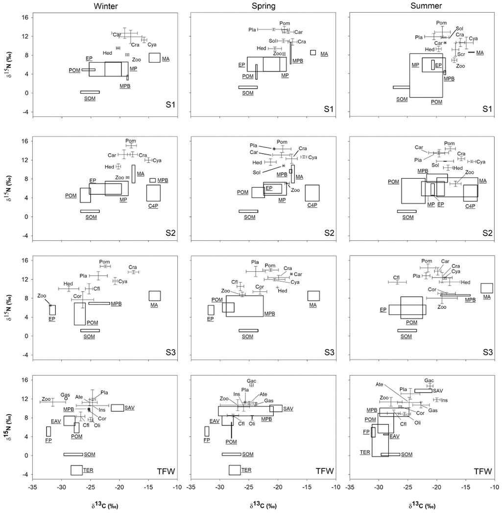
Average (±SD) δ¹⁵N and δ¹³C values (‰) of pelagic, benthic, and epibenthic consumers in the brackish (S1-S3) and freshwater (TFW) areas of the Minho River estuary during winter (high river discharge), spring (intermediate river discharge), and summer 2011 (low river discharge). The consumers shown are zooplankton (Zoo), Scrobicularia plana (Scr), Hediste diversicolor (Hed), Cyathura carinata (Cya), Corophium sp. (Cor), Corbicula fluminea (Cfl), Insect larvae (Ins), Oligochaeta (Oli), Gastropoda (Gas), Crangon crangon (Cra), Carcinus maenas (Car), Atyaephyra desmaresti (Ate), Pomatoschistus microps (Pom), Platichthys flesus (Pla), Solea solea (Sol), and Gasterosteus aculeatus (Gac). Boxes represent the average and SD for the organic matter sources collected during this study, and also the estimates for C4 saltmarsh plants and phytoplankton (see text for references): marine (MP), estuarine (EP), and freshwater (FP) phytoplankton, particulate organic matter (POM), macroalgae (MA), sediment organic matter (SOM), microphytobenthos (MPB), C4 plants (C4P) and other emergent aquatic vegetation (EAV), submerged aquatic vegetation (SAV), and terrestrial plants (TER).

3.2. Food web characterization

In S1 and S2, FF and DF consumers relied on a mixture of marine and brackish phytoplankton, macroalgae detritus, and benthic OM (MPB and SOM) (Fig. 2). Based on the stable isotope ratio bi-plot analysis, zooplankton, polychaetes, and C. carinata consumed a mix of phytoplankton, MPB, macroalgae, and plant detritus (Fig. 3). However, the high δ¹⁵N and δ¹³C values of C. carinata (S1 and S2) and polychaetes (S2) suggest either carnivory or increasing proportional contribution of ¹⁵N-enriched material due to microbial processing (Fig. 3; Goedkoop et al., 2006). In S3, the high δ¹³C values of some consumers (Corophium sp., polychaetes, C. carinata), particularly during summer, suggest the contribution of marine POM to the central portion of the estuary (Fig. 3). The FF and DF likely consumed POM and phytoplankton (marine, estuarine, or freshwater) because their δ¹³C values are intermediate between POM and phytoplankton (Fig. 3). In the TFW area, benthic consumers had similar δ¹³C and δ¹⁵N values during winter and spring; the isotopic composition indicated they were feeding on a mixture of sources, including POM, MPB, and detritus (Fig. 3). Phytoplankton was not a relevant contributor to benthic consumers’ biomass because they were too ¹³C-enriched to rely on freshwater phytoplankton (> 5‰) and too ¹³C- depleted to rely on estuarine phytoplankton (ca. 5‰; Fig. 3). Based on their stable isotope ratios, they were likely feeding on a mixture of plant detritus and OM in the sediment (i.e., SOM and MPB) throughout the study (Fig. 3).

Based on the dual-stable isotope mixing model, most benthic consumers collected during this study relied on phytoplankton, vascular plant detritus, and MPB (Fig. 4; model contribution estimates and associated errors are provided in Table A.1). However, their respective proportional contributions varied both spatially and temporally. Phytoplankton’s proportional contribution was higher in the stations closer to the river mouth and was more relevant for filter feeders and polychaetes (Table A.1). The relative contribution of marine phytoplankton to the consumers analyzed was, in general, higher than that of estuarine or freshwater and during spring (Fig. 4). The contribution of estuarine phytoplankton was higher during winter than in the other seasons, while the contribution of freshwater phytoplankton increased during summer (Fig. 4). Benthic consumers and zooplankton from the saltmarsh (S2) and TFW relied mainly on the detrital food web, regardless of season, either through the direct consumption of vascular detritus and terrestrial-derived POM or indirectly through microbially-processed OM, or both (Fig. 4, Table A.1). MPB contributed to the biomass of all consumers collected across the estuary, but especially to those in S1 and S3 (Fig. 4). The number of sources assimilated by these consumers increased upriver (Fig. 4).

Fig. 4.

Average mode values of the relative contribution (%) of each organic matter source to the deposit feeders (DF) and filter feeders (FF) collected along the salinity gradient of the Minho River estuary during winter, spring, and summer of 2011, based on the dual-stable isotope mixing model. Organic matter (OM) sources include: marine (MP), estuarine (EP), and freshwater phytoplankton (FP), particulate OM (POM), macroalgae (MA), microphytobenthos (MPB), sediment OM (SOM), emergent (EAV, including C4 plants) and submerged aquatic vegetation (SAV). The OM sources selected for each taxon are present in Table A.1.

Allochthonous subsidies (i.e., OM originated in adjacent habitats or ecosystems: marine and freshwater phytoplankton, macroalgae, terrestrial-derived POM) are relevant to the Minho estuary benthic food web, and its importance increased upriver during winter and spring, following the opposite pattern during summer (Fig. 5). The highest contribution of allochthonous subsidies was observed in S1 during spring (78.3%) and in S2 during summer (80.3%; Fig. 5). The contribution of autochthonous sources (including SOM) increased upriver during summer and was higher in the middle estuary (S3) than in the lower estuary (S1 and S2) during spring. (Fig. 5). The highest values were observed in S3 during spring (63.5%) and in TFW during summer (61.1%; Fig. 5).

Fig. 5.

Average mode values of the relative contribution (%) of organic matter source, according to origin (allochthonous or autochthonous), to the filter feeders and deposit feeders collected along the salinity gradient of the Minho River estuary during winter, spring, and summer of 2011.

The length of the benthic food web in the Minho estuary (given by the trophic position (TP) of the epibenthic consumers) consisted of four trophic levels, with the TP values varying between 2.0 (P. flesus in TFW during summer) and 4.6 (P. microps in S3 during winter). The lowest average TP values were observed in TFW and the highest in S2 (Fig. 6; ART: F_(2,405) = 10.0, p < 0.05). Overall, TP median values were higher during spring and summer than during winter (Fig. 6; ART: F_(3,405) = 60.0, p < 0.05). No significant relationship was found between TP and the size for each species (Fig. A.1; sizes were not available for the species G. aculeatus and S. solea), but the highest TP values were associated to low Chl a concentrations (Figs. 2 and 6).

Fig. 6.

Box plots depicting comparisons of food-chain lengths among stations and seasons in the Minho estuary. Median (solid line within box), quartiles (box) and range (whiskers) are presented for each factor.

4. Discussion

Two trophic pathways were recognized in the Minho estuary food web. The first was a pathway supported by phytoplankton and composed of filter feeders such as zooplankton and deposit feeders, especially amphipods and polychaetes. The second pathway was supported by detritus and composed of deposit feeders such as insect larvae, oligochaetes, gastropods, and small shrimps. A detritus-based, microbial food web likely mediates part of this energy transfer to estuarine consumers. Which of the two pathways were dominant varied by location along the estuary and season. The contribution of phytoplankton to the benthic food web was highest in the brackish estuary and increased during the spring and summer. In contrast, the contribution of detritus to estuarine consumers was highest in tidal freshwater (TFW) areas and in the saltmarsh, especially during spring. There was no clear relationship between the epibenthic consumers’ trophic position (TP) and the main trophic pathways, but TP decreased with increasing Chl a concentration. The observed changes along the estuarine salinity gradient and possible mechanisms responsible for the cross-ecosystems food web linkages are discussed below.

4.1. Spatial heterogeneity of the estuarine food web

Terrestrial plants presented typical δ¹³C values of ca. −28‰ because they uptake carbon from the atmosphere (Peterson and Fry, 1987). Contrarily, aquatic primary producers, which uptake DIC from solution, display variable δ¹³C values corresponding to variability in δ¹³C_DIC, which usually increases as salinity increases (Chanton and Lewis, 2002; Fry, 2002; Dias et al., 2016). Thus, the aquatic primary producers which obtain inorganic carbon from solution will often have a δ¹³C value corresponding to the portion of the estuary where they were collected. Regions of intense production (¹³C-enriched) or respiration (¹³C-depleted), such as the estuarine turbidity maximum, may demonstrate a shift in δ¹³C_DIC values (±1.5 ‰; Su et al., 2019), potentially shifting the isotopic composition of primary products towards other sources. However, given the large δ¹³C value range among sources and lack of known strong production gradients within the Minho estuary, we do not have reason to believe δ¹³C_DIC values are substantially confounding interpretation of sources in this study.

Consumers relying on benthic or detrital C, such as isopods and insect larvae, were generally more ¹⁵N- and ¹³C- enriched than those that relied mainly on OM sources in the phytoplankton pathway, such as zooplankton or amphipods. Plausibly, this is due to the incorporation of benthic algae, which have higher δ¹³C values than phytoplankton, which has been attributed to the existence of a diffusive boundary layer at the sediment-water interface that reduces carbon isotopic fractionation (France, 1995). Alternatively, detrital carbon is subject to microbial degradation, which enriches the OM in ¹³C and ¹⁵N (Goedkoop et al., 2006). Both processes are likely operating in the estuary.

In TFW, terrestrial-derived OM also contributed to filter feeders (FF) and deposit feeders (DF), especially during winter and spring. This is likely the result of a physical export of OM (detritus and POM) from upland or upriver to the estuarine habitats. Their δ¹³C values mirrored the patterns in the δ¹³C POM values, which were ¹³C- depleted towards the freshwater environments due to an increase in the contribution of ¹³C- depleted terrestrial and riverine material, as indicated by the isotopic composition and C:N value of riverine POM. In the brackish estuary, marine phytoplankton (or MPOM) was an important energy source to FF and DF owing to marine intrusion.

Between-habitat differences in the stable isotope ratios of primary consumers was overall reflected in the isotopic ratios of epibenthic consumers, which were also ¹³C-enriched towards the river mouth.

4.2. Temporal variability in the estuarine food web

Temporal variation was observed in the POM pool. The δ¹³C_POC values increased towards summer in the brackish portion of the estuary, while the opposite pattern was observed in stations located in the TFW. During winter, when the river discharge is high (400–600 m³.s⁻¹; Fig. 2 in Dias et al., 2016), the δ¹³C_POC values (δ¹³C: −28‰ to – 24‰) and C:N_POM ratio (> 10) suggest a substantial contribution of terrestrial-derived OM to the POM pool, advected from upland or riparian habitats, or both (Hedges et al., 1997; Hoffman et al., 2008). The low Chl a concentrations (0.8 ± 0.8 μg L⁻¹) during this period also suggest that the contribution of phytoplankton to the POM pool decreased owing to the suppression of primary production as a consequence of increased turbidity and rapid flushing rates (Sin et al., 1999; Hoffman and Bronk, 2006). During summer, river discharge declined (< 200 m³s⁻¹; Fig. 2 in Dias et al., 2016), which decreases terrestrial inputs to the estuary and increases the residence time. This promotes the accumulation of living and detrital phytoplankton in freshwater and areas under strong marine influence (Hoffman and Bronk, 2006; Dias et al., 2016). Our results suggest that during summer, especially in August 2011, there was an increase in the contribution of phytoplankton to the POM pool. The concentration of Chl a increased during summer, peaking in August 2011 in the TFW stations (concentrations up to 8 times higher than in the other months) and in the middle estuary (up to 6 times), suggesting the occurrence of a phytoplankton bloom during this month (Dias et al., 2016). Moreover, the δ¹³C_POC values in the TFW (δ¹³C_POC: −30‰) were similar to those estimated for freshwater phytoplankton in this estuary (δ¹³C: −31‰; Dias et al., 2016) and the C:N_POM was lower than 10, indicating a decrease in the contribution of terrestrial-derived OM to the POM pool.

The temporal variability of the POM pool was reflected in the stable isotope ratios of FF and some DF (e.g., amphipods, polychaetes), indicating that during high river discharge conditions, the estuarine benthic food web incorporated terrestrial-derived OM, as observed elsewhere (Antonio et al., 2012). Moreover, benthos consumption of terrestrial-derived OM may have a significant impact on the use of decomposed terrestrial-derived OM because bacterial colonization and growth can improve the quality of POM, even for terrestrial-derived detritus (Edwards and Meyer, 1987), potentially enhancing terrestrial material transfer in aquatic food webs (Zeug and Winemiller, 2008; Dias et al., 2014).

Although isotopic baseline changes induced variability in the stable isotope ratios of some primary consumers, we found differences that were likely related to variability in feeding strategies. For example, during the summer in S3, Cyathura carinata and Hediste diversicolor had higher δ¹⁵N values (ca. 6‰) than average MPB δ¹⁵N values, which was the most ¹⁵N-enriched source sampled. The difference between the δ¹⁵N values of these consumers and MPB was almost two trophic levels (assuming typical fractionation of + 3.4‰ for δ¹⁵N and + 0.5‰ for δ¹³C; Vander Zanden and Rasmussen, 2001). We suggest three possible explanations: 1) they were feeding on the microbially-mediated food web, 2) the trophic fractionation values used were not appropriate, or 3) C. carinata and H. diversicolor were preying on primary consumers. Station 3 is located in the transition between marine and freshwaters (Dias et al., 2016). Although an estuarine turbidity maximum (ETM) has not been identified yet in this estuary, the ETM is a zone of elevated turbidity near the landward limit of salt intrusion (Geyer, 1993; Jay and Musiak, 1994; Sanford et al., 2001, 2005) where phytoplankton, bacteria, and detritus tend to accumulate (Herman and Heip, 1999), and where POM is extensively reprocessed by bacteria (Goosen et al., 1999). This can cause ¹⁵N- enrichment of the available POM pool. However, if that was the case, that ¹⁵N-enrichment would be reflected in other consumers such as C. fluminea. Recent studies suggest that the trophic fractionation of H. diversicolor may be higher than the average values commonly used in aquatic food web studies, + 1.6‰ for δ¹³C and + 5.0‰ for δ¹⁵N values (Kristensen et al., 2019). However, these values were estimated using sediment organic matter as the baseline, and our study indicates that H. diversicolor rely on both phytoplankton and detritus. Thus, because trophic fractionation can vary according food quality (Vander Zanden and Rasmussen, 2001; Caut et al., 2009) and because previous studies indicate that H. diversicolor and C. carinata can prey on other animals (Wägele et al., 1981; Nordström et al., 2009), we consider that either explanation is possible. Nonetheless, both explanations yield similar relative proportional contributions of the most likely OM sources.

4.3. Food web modeling

One critical assumption of food web reconstruction based on stable isotope ratios is that the OM source values measured are temporally aligned with the isotopic turnover period of the organisms sampled. In invertebrates, isotopic half-life (i.e., time required to reach 50% equilibration with the diet) generally increases with animal body mass (Vander Zanden et al., 2015). Although isotopic turnover estimates for the species analyzed in this study are lacking, small invertebrates such as zooplankton (Hoffman et al., 2007), mussels (Dubois et al., 2007), and shrimps (Fry and Arnold, 1982) have isotopic half-life estimates of less than one month. That is, they integrate seasonal or even within-season isotopic variability of their diet. It also indicates that the stable isotope approach is responsive to seasonal environmental processes (e. g., watershed inputs).

Another critical aspect was that this study used estimates obtained elsewhere for marine plytoplankton and C4 plants. The estimates for marine phytoplankton were obtained from coastal areas near the Minho River (Bode et al., 2007; McMahon et al., 2013). Although McMahon et al. (2013) lack a temporal component, they estimated that phytoplankton isotope values are similar between Galicia and the North of Portugal. Moreover, the δ¹³C values in the studies mentioned above are similar to estimates obtained previously for this study area (Dias et al., 2014, 2016), suggesting that phytoplankton stable isotope values could be similar between close geographic areas. The values used for C4 plants include the typical ranges found in other estuarine ecosystems (e.g., Fry and Sherr, 1984; Deegan and Garritt, 1997; Cloern et al., 2002; Dias et al., 2019a). Similar estimates were obtained for C4 plants in the Minho estuary in a previous study: −13.9 ± 0.5‰ for δ¹³C and 7.1 ± 0.4 δ¹⁵N (Fig. 2, Dias et al., 2020). Because the estimates were obtained in 2015 and the dispersion was low, we used a broader range of values to accommodate potential temporal differences in the stable isotope values.

4.4. Food chain length

The average food-chain length varied between 2.7 (TFW) and 3.6 (S2), and within-station variation was the highest in S1 and S2. Also, the food chain length varied temporally, with higher median values observed during spring (S2 and TFW) and summer (S1 and S3) than in winter. It is important to note that similar epibenthic predators’ assemblages occurred in all stations, although the number of species analyzed was lower in the upper estuary (TFW) when compared to the low (S1-S2) and middle estuary (S3). Thus, longer food chains correspond to more trophic transfers and not to adding more species to the top. Also, this study focused on the most abundant epibenthic predators in the Minho estuary, not including others such as the European eel, which prey on insects, crustaceans, and other fish (e.g., Costa et al., 1992). Adding this species would likely increase the size of the benthic food chain; nonetheless, this species occurs throughout the estuary, and thus, its role as a predator is expected to be similar across the sampled area.

It has been hypothesized that as the contribution of detritus increases, the food chain length decreases, while the opposite trend is expected to occur in food webs fueled by phytoplankton (Hoeinghaus et al., 2008). However, the contribution of detritus to macroinvertebrates was higher in S2 and TFW than in the other stations, but the food chain length was the highest and the lowest, respectively, suggesting that energy quality probably does not influence the length of the benthic food web in the Minho estuary. Regarding food quantity, although there are no estimates for the primary productivity in this ecosystem, average Chl a concentrations were overall higher in TFW and during the summer. Elton (1927) predicted, and others concluded (e.g., Thompson and Townsend, 2005; Qin et al., 2021) that more productive ecosystems should have longer food chains. Here, food chains were shorter in habitats with high Chl a concentrations, and no clear temporal relationship was found between these two variables; food chain length was higher in spring or summer and varied according to the station. However, predator foraging adaptation (e.g., feeding behavioral plasticity) can mask the effects of increasing resource variability on the food chain length; predators will tend to feed on lower trophic level prey with increasing resource availability resulting in shorter food chains (Kondoh and Ninomiya, 2009). This effect could partially explain our findings since all the epibenthic predators analyzed in this study are considered generalist predators (e.g., Pihl, 1985; Jackson et al., 2004), but further specific studies are necessary to test the relationship between resource availability and predators’ diet and trophic position in the Minho estuary. Community complexity (e.g., species richness) can positively relate to food chain length (Kondoh and Ninomiya, 2009). To the best of our knowledge, only one study analyzed macroinvertebrates’ diversity across the Minho estuary salinity gradient (Sousa et al., 2008). Here, it was found that species richness is the lowest in the middle estuary increasing towards the lower and upper limits of the estuary (Sousa et al., 2008). Despite that the community evenness (J’) is lower in the upper estuary than in the other areas (Sousa et al., 2008) indicating that a few species dominate these communities. In the Minho estuary, these areas are dominated by the invasive gastropod Potamopyrgus antipodarum and especially by the invasive clam Corbicula fluminea (Sousa et al., 2008). In fact, this clam accounts for >90% of the total macroinvertebrate biomass at the middle and upper estuary (Sousa et al., 2005, 2008). Given its high filtering capacity (Strayer et al., 1999) and flexible feeding strategy (Dias et al., 2014), we hypothesize that this species may have induced a simplification of the food web structure upriver by shortening the food chain (Maceda-Veiga et al., 2018) and by decreasing trophic functional diversity (dominance of deposit feeders and detritivores). However, no information on the food web structure in the Minho River is available prior to the invasion of this clam, and thus, the role of invasive species in the food web structure deserves further attention.

5. Conclusions

This study provides evidence for spatial and temporal variability in the dominant trophic pathways in the Minho River estuarine benthic food web. The phytoplankton pathway was more relevant for filter-feeding animals and some deposit feeders, indicating that benthic-pelagic coupling processes play an essential role in the energy transfer to the benthic food web. The detrital pathway was more relevant for deposit-feeding organisms in the saltmarsh and freshwater areas, especially during the winter and spring, where the food chain length was the highest and the lowest, respectively. This indicates that energy quality probably does not influence the length of the benthic food web in the Minho estuary. The magnitude of river inflow and marine intrusion moving in the opposite direction drove the energy subsidy dynamics between the estuary and its adjacent ecosystems (i.e., land and sea), which was then mirrored in the OM sources assimilated by the consumers analyzed. Thus, this study highlights the role of benthic consumers in linking the estuarine food web with terrestrial and marine ecosystems. Because they can consume both pelagic and benthic OM sources, they also facilitate the connectivity between benthic and pelagic habitats.

References

- Alves AM, 1996. Causas e processos da dinâmica sedimentar na evolução actual do litoral do Alto Minho. PhD Dissertation. Universidade do Minho. [Google Scholar]
- Antonio ES, Kasai A, Ueno M, Ishihi Y, Yokoyama H, Yamashita Y, 2012. Spatiatemporal feeding dynamics of benthic communities in an estuary-marine gradient. Estuar. Coast. Shelf Sci 112, 86–97. [Google Scholar]
- Antunes C, Araújo MJ, Braga C, Roleira A, Carvalho R, Mota M, 2011. Valorização dos recursos naturais da bacia hidrográfica do rio Minho. Final report from the project Natura Miño-Minho, Centro interdisciplinar de Investigação Marinha e Ambiental. Universidade do Porto. [Google Scholar]
- Atkinson CL, First MR, Covich AP, Opsahl SP, Golladay SW, 2011. Suspended material availability and filtration-biodeposition processes performed by a native and invasive bivalve species in streams. Hydrobiologia 667, 191–204. [Google Scholar]
- Bergamino L, Richoux NB, 2015. Spatial and temporal changes in estuarine food web structure: differential contributions of marsh grass detritus. Estuar. Coasts 38, 367–382. [Google Scholar]
- Bode A, Alvarez-Ossorio MT, Varela M, 2006. Phytoplankton and macrophyte contributions to littoral food webs in the Galician upwelling estimated from stable isotopes. Mar. Ecol. Prog. Ser 318, 89–102. [Google Scholar]
- Bode A, Alvarez-Ossorio MT, Cunha ME, Garrido S, Peleteiro JB, Porteiro C, Valdés L, Varela M, 2007. Stable nitrogen isotope studies of the pelagic food web on the Atlantic shelf of the Iberian Peninsula. Prog. Oceanogr 74, 115–131. [Google Scholar]
- Brito AC, Brotas V, Caetano M, Coutinho TP, Bordalo AA, Icely J, Neto JM, Serôdio J, Moita T, 2012. Defining phytoplankton class boundaries in Portuguese transitional waters: an evaluation of the ecological quality status according to the water framework directive. Ecol. Indic 19, 5–14. [Google Scholar]
- Canuel EA, Cloern JE, Ringelberg DB, Guckert JB, 1995. Molecular and isotopic tracers used to examine sourcesof organic matter and its incorporation into the food websof San Francisco Bay. Limnol. Oceanogr 40, 67–81. [Google Scholar]
- Carpenter SR, Cole ML, Pace M, Van de Bogert M, Bade DL, Bastviken D, Gille JR, Hodgson JF, Kritzberg ES, 2005. Ecosystem subsidies: terrestrial support of 361 aquatic food web from 13C addition to contrasting lakes. Ecology 86, 2737–2750. [Google Scholar]
- Caut S, Angulo E, Courchamp F, 2009. Variation in discrimination factors (Δ15N and Δ13C): the effect of diet isotopic values and applications for diet reconstruction. J. Appl. Ecol 46, 443–453. [Google Scholar]
- Chanton J, Lewis FG, 2002. Examination of coupling between primary and secondary production in a river-dominated estuary: Apalachicola Bay, Florida, USA. Limnol. Oceanogr 47, 683–697. [Google Scholar]
- Cloern JE, Canuel EA, Harris D, 2002. Stable carbon and nitrogen isotope composition of aquatic and terrestrial plants of the San Francisco Bay estuarine system. Limnol. Oceanogr 47, 713–729. [Google Scholar]
- Costa JL, Almeida PR, Moreira FM, Costa MJ, 1992. On the food of the European eel, Anguilla anguilla (L.), in the upper zone of the Tagus estuary, Portugal. J. Fish Biol 41, 841–850. [Google Scholar]
- Costa-Dias S, Freitas V, Sousa R, Antunes C, 2010. Factors influencing epibenthic assemblages in the Minho estuary (NW Iberian Peninsula). Mar. Pollut. Bull 61, 240–246. [DOI] [PubMed] [Google Scholar]
- Currin CA, Newell SY, Paerl HW, 1995. The role of standing dead Spartina alterniflora and benthic microalgae in salt marsh food webs: considerations based on multiple stable analysis. Mar. Ecol. Prog. Ser 121, 99–116. [Google Scholar]
- Deegan LA, Garritt RH, 1997. Evidence for spatial variability in estuarine food webs. Mar. Ecol. Prog. Ser 147, 31–47. [Google Scholar]
- DeNiro MJ, Epstein S, 1977. Mechanism of carbon isotope fractionation associated with lipid synthesis. Science 197, 261–263. [DOI] [PubMed] [Google Scholar]
- Dias E, Morais P, Antunes C, Hoffman JC, 2014. Linking terrestrial and benthic estuarine ecosystems: organic matter sources supporting the high secondary production of a non-indigenous bivalve. Biol. Invasions 16, 2163–2179. [Google Scholar]
- Dias E, Morais P, Cotter AM, Antunes C, Hoffman JC, 2016. Estuarine consumers utilize marine, estuarine and terrestrial organic matter and provide connectivity among these food webs. Mar. Ecol. Prog. Ser 554, 21–34. [Google Scholar]
- Dias E, Chainho P, Barrocas-Dias C, Adão H, 2019a. Food sources of the non-indigenous bivalve Ruditapes philippinarum (Adams and Reeve, 1850) and trophic niche overlap with native species. Aquat. Invasions 14, 638–655. [Google Scholar]
- Dias E, Miranda ML, Sousa R, Antunes C, 2019b. Riparian vegetation subsidizes sea lamprey ammocoetes in a nursery area. Aquat. Sci 81, 44. [Google Scholar]
- Dias E, Barros AG, Hoffman JC, Antunes C, Morais P, 2020. Habitat use and food sources of European flounder larvae (Platichthys flesus, L.1758) across the Minho River estuary salinity gradient (NW Iberian Peninsula). Reg. Stud. Mar. Sci 34, 101196. [DOI] [PMC free article] [PubMed] [Google Scholar]
- Dubois SF, Jean-Louis B, Bertrand B, Lefebvre S, 2007. Isotope trophic-step fractionation of suspension-feeding species: implications for food partitioning in coastal ecosystems. J. Exp. Mar. Biol. Ecol 351, 121–128. [Google Scholar]
- Edwards RT, Meyer JL, 1987. Bacteria as a food source for black fly larvae in a blackwater river. J. N. Am. Benthol. Soc 6, 241–250. [Google Scholar]
- Elton CS, 1927. Animal Ecology. Sidgwick and Jackson. [Google Scholar]
- Ferreira JG, Simas T, Nobre A, Silva MC, Schifferegger K, Lencart-Silva J, 2003. Identification of sensitive areas and vulnerable zones in transitional and coastal Portuguese systems. Application of the United States National Estuarine Eutrophication Assessment to the Minho, Lima, Douro, Ria de Aveiro, Mondego, Tagus, Sado, Mira, Ria Formosa and Guadiana systems. INAG/IMAR Technical Report. [Google Scholar]
- Feuchtmayer H, Grey J, 2003. Effect of preparation and preservation procedures on carbon and nitrogen stable isotope determinations from zooplankton. Rapid Commun. Mass Spectrom 17, 2605–2610. [DOI] [PubMed] [Google Scholar]
- France RL, 1995. Carbon-13 enrichment in benthic compared to planktonic algae: foodweb implications. Mar. Ecol. Prog. Ser 124, 307–312. [Google Scholar]
- Fry B, 2002. Conservative mixing of stable isotopes across estuarine salinity gradients: a conceptual framework for monitoring watershed influences on downstream fisheries production. Estuaries 25, 264–271. [Google Scholar]
- Fry B, Arnold C, 1982. Rapid 13C/12C turnover during growth of brown shrimp (Penaeus aztecus). Oecologia 54, 200–204. [DOI] [PubMed] [Google Scholar]
- Fry B, Sherr EB, 1984. δ13C measurements as indicators of carbon flow in marine and freshwater ecosystems. Contrib. Mar. Sci 27, 15–47. [Google Scholar]
- Fry B, Baltz DB, Benfield MC, Fleeger JW, Gace A, Haas HL, Quiñones-Rivera ZJ, 2003. Stable isotope indicators of movement and residency for brown shrimp (Farfantepenaeus aztecus) in coastal Louisiana marshscapes. Estuaries 26, 82–97. [Google Scholar]
- Gerdol V, Hughes RG, 1994. Feeding behavior and diet of Corophium volutator in an estuary in southeastern England. Mar. Ecol. Prog. Ser 114, 103–108. [Google Scholar]
- Geyer WR, 1993. The importance of suppression of turbulence by stratification on the estuarine turbidity maximum. Estuaries 16, 113–125. [Google Scholar]
- Goedkoop W, Akerblom N, Demandt MH, 2006. Trophic fractionation of carbon and nitrogen stable isotopes in Chironomus riparius reared on food of aquatic and terrestrial origin. Freshw. Biol 51, 878–886. [Google Scholar]
- Goosen NK, Kromkamp J, Peene J, van Rijswijk P, van Breugel P, 1999. Bacterial and phytoplankton production in the maximum turbidity zone of three European estuaries: the Elbe, Westerschelde and Gironde. J. Mar. Syst 22, 151–171. [Google Scholar]
- Hedges JI, Clark WA, Quay PD, Richey JE, Devol AH, Santos UM, 1986. Compositions and fluxes of particulate organic material in the Amazon River. Limnol. Oceanogr 31, 717–738. [Google Scholar]
- Hedges JI, Keil RG, Benner R, 1997. What happens to terrestrial organic matter in the ocean? Org. Geochem 27, 195–212. [Google Scholar]
- Herman PMJ, Heip CHR, 1999. Biogeochemistry of the MAximum TURbidity zone of estuaries (MATURE): some conclusions. J. Mar. Syst 22, 89–104. [Google Scholar]
- Hoeinghaus DJ, Winemiller KO, Agostinho AA, 2008. Hydrogeomorphology and river impoundment affect food-chain length of diverse Neotropical food webs. Oikos 117, 984–995. [Google Scholar]
- Hoffman JC, Bronk DA, 2006. Interannual variation in stable carbon and nitrogen isotope biogeochemistry of the Mattaponi River, Virginia. Limnol. Oceanogr 51, 2319–2332. [Google Scholar]
- Hoffman JC, Sutton TT, 2010. Lipid correction for carbon stable isotope analysis of deep-sea fishes. Deep-Sea Res. I 57, 956–964. [Google Scholar]
- Hoffman JC, Bronk DA, Olney JE, 2007. Tracking nursery habitat use by young American shad in the York River estuary, Virginia, using stable isotopes. Trans. Am. Fish. Soc 136, 1285–1297. [Google Scholar]
- Hoffman JC, Bronk DA, Olney JE, 2008. Organic matter sources supporting lower food web production in the tidal freshwater portion of the York River estuary, Virginia. Estuar. Coasts 31, 898–911. [Google Scholar]
- Hoffman JC, Kelly JR, Peterson GS, Cotter AM, 2015. Landscape-scale food webs of fish nursery habitat along a river-coast mixing zone. Estuar. Coasts 38, 1335–1349. [Google Scholar]
- Howe ER, Simenstad CA, 2015. Using stable isotopes to discern mechanisms of connectivity in estuarine detritus-based food webs. Mar. Ecol. Prog. Ser 518, 13–29. [Google Scholar]
- Hughes JE, Deegan LA, Peterson BJ, Holmes RM, Fry B, 2000. Nitrogen flow through the food web in the oligohaline zone of a new England estuary. Ecology 81, 433–431. [Google Scholar]
- Huxel GR, McCann K, 1998. Food web stability: the influence of trophic flows across habitats. Am. Nat 152, 460–469. [DOI] [PubMed] [Google Scholar]
- Jackson AC, Rundle SD, Attrill MJ, Cotton PA, 2004. Ontogenetic changes in metabolism may determine diet shifts for a sit-and-wait predator. J. Anim. Ecol 73, 536–545. [Google Scholar]
- Jay DA, Musiak JD, 1994. Particle trapping in estuarine tidal flows. J. Geophys. Res 99, 20445–20461. [Google Scholar]
- Kang CK, Kim JB, Lee KS, Kim JB, Lee PY, Hong JS, 2003. Trophic importance of benthic microalgae to macrozoobenthos in coastal bay systems in Korea: dual stable C and N isotopes analyses. Mar. Ecol. Prog. Ser 259, 79–92. [Google Scholar]
- Kasai A, Nakata A, 2005. Utilization of terrestrial organic matter by the bivalve Corbicula japonica estimated from stable isotope analysis. Fish. Sci 71, 151–158. [Google Scholar]
- Kay M, Elkin L, Higgins J, Wobbrock J, 2021. ARTool: Aligned Rank Transform for Nonparametric Factorial ANOVAs. 10.5281/zenodo.594511. [DOI] [Google Scholar]
- Keats RA, Osher LJ, Neckles HA, 2004. The effect of nitrogen loading on a brackish estuarine faunal community: a stable isotope approach. Estuaries 27, 460–471. [Google Scholar]
- Kleppel GS, 1993. On the diets of calanoid copepods. Mar. Ecol. Prog. Ser 99, 183–195. [Google Scholar]
- Kohler AE, Pearsons TN, Zendt JS, Mesa MG, Johnson CL, Connolly PJ, 2012. Nutrient enrichment with salmon carcass analogs in the Columbia River Basin, USA: a stream food web analysis. Trans. Am. Fish. Soc 141, 802–824. [Google Scholar]
- Kondoh M, Ninomiya K, 2009. Food-chain length and adaptive foraging. Proc. R. Soc. B 276, 3113–3121. [DOI] [PMC free article] [PubMed] [Google Scholar]
- Kristensen E, Quintana CO, Valdemarsen T, 2019. Stable C and N stable isotope composition of primary producers and consumers along an estuarine salinity gradient: tracing mixing patterns and trophic discrimination. Estuar. Coasts 42, 144–156. [Google Scholar]
- Lorenzen CJ, 1967. Determination of chlorophyll and pheo-pigments: spectrophotometric equations. Limnol. Oceanogr 12, 343–346. [Google Scholar]
- Lorrain A, Savoye N, Chauvaud L, Paulet Y-M, Naulet N, 2003. Decarbonation and preservation method for the analysis of organic C and N contents and stable isotope ratios of low-carbonated suspended particulate material. Anal. Chim. Acta 491, 125–133. [Google Scholar]
- Lucero RCH, Cantera KJR, Romero IC, 2006. Variability of macrobenthic assemblages under abnormal climatic conditions in a small scale tropical estuary. Estuar. Coast. Shelf Sci 68, 17–26. [Google Scholar]
- Maceda-Veiga A, Nally RM, de Sostoa A, 2018. Environmental correlates of food-chain length, mean trophic level and trophic level variance in invaded riverine fish assemblages. Sci. Total Environ 644, 420–429. [DOI] [PubMed] [Google Scholar]
- McMahon K, Hamady LL, Thorrold SR, 2013. A review of ecogeochemistry approaches to estimating movements of marine animals. Limnol. Oceanogr 58, 697–714. [Google Scholar]
- Minagawa M, Wada E, 1984. Stepwise enrichment of 15N along food chains: further evidence and the relation between δ15N and animal age. Geochim. Cosmochim. Acta 48, 1135–1140. [Google Scholar]
- Nordström M, Aarnio K, Bonsdorff E, 2009. Temporal variability of a benthic food web: patterns and processes in a low-diversity system. Mar. Ecol. Prog. Ser 378, 13–26. [Google Scholar]
- Parnell AC, Inger R, Bearhop S, Jackson AL, 2010. Source partitioning using stable isotopes: coping with too much variation. PlosOne 5, e9672. [DOI] [PMC free article] [PubMed] [Google Scholar]
- Pestana JLT, Ré A, Nogueira AJ, Soares AMVM, 2007. Effects of Cadmium and Zinc on the feeding behaviour of two freshwater crustaceans: Atyaephyra desmarestii (Decapoda) and Echinogammarus meridionalis (Amphipoda). Chemosphere 68, 1556–1562. [DOI] [PubMed] [Google Scholar]
- Peterson BJ, Fry B, 1987. Stable isotopes in ecosystem studies. Annu. Rev. Ecol. Syst 18, 293–320. [Google Scholar]
- Pihl L, 1985. Food selection and consumption of mobile epibenthic fauna in shallow marine areas. Mar. Ecol. Prog. Ser 22, 169–179. [Google Scholar]
- Polis GA, Anderson WB, Holt RD, 1997. Toward an integration of landscape and food web ecology: the dynamics of spatially subsidized food webs. Annu. Rev. Ecol. Syst 28, 289–316. [Google Scholar]
- Post DM, 2002a. Using stable isotopes to estimate trophic position: models, methods, and assumptions. Ecology 83, 703–718. [Google Scholar]
- Qin Q, Zhang F, Wang C, Huanzhang L, 2021. Food web structure and trophic interactions revealed by stable isotope analysis in the midstream of the Chishui River, a tributary of the Yangtze River, China. Water 13, 195. [Google Scholar]
- R Core Team, 2020. R: A language and environment for statistical computing. R Foundation for Statistical Computing, Vienna, Austria. [Google Scholar]
- Riley RH, Townsend CR, Raffaelli DA, Flecker AS, 2004. Sources and effects of subsidies along the stream-estuary continuum. In: Polis GA, Power ME, Huxel GR (Eds.), Food Webs at the Landscape Level. The University of Chicago Press, Chicago, pp. 241–260. [Google Scholar]
- Rooney N, McCann KS, 2011. Integrating food web diversity, structure and stability. Trends Ecol. Evol 27, 40–46. [DOI] [PubMed] [Google Scholar]
- Sanford LP, Suttles SE, Halka JP, 2001. Reconsidering the physics of the Chesapeake Bay estuarine turbidity maximum. Estuaries 24, 655–669. [Google Scholar]
- Sanford LP, Dickhudt L, Rubiano-Gomez M, Yates S, Suttles S, Friedrichs CT, Fugate DD, Romaine H, 2005. Variability of suspended particle concentrations, sizes and settling velocities in the Chesapeake Bay turbidity maximum. In: Droppo IG, Leppard GG, Liss SN, Milligan TG (Eds.), Flocculation in Natural and Engineered Environmental Systems. CRC Press, Florida, pp. 210–236. [Google Scholar]
- Schindler DE, Scheuerell MD, Moore JW, Gende SM, Francis TB, Palen WJ, 2003. Pacific salmon and the ecology of coastal ecosystems. Front. Ecol. Environ 1, 31–37. [Google Scholar]
- Selleslagh J, Blanchet H, Bachelet G, Lobry J, 2015. Feeding habitats, connectivity and origin of organic matter supporting fish populations in an estuary with a reduced intertidal area assessed by stable isotope analysis. Estuar. Coasts 38, 1431–1447. [Google Scholar]
- Sheaves M, 2009. Consequences of ecological connectivity: the coastal ecosystem mosaic. Mar. Ecol. Prog. Ser 391, 107–115. [Google Scholar]
- Sin Y, Wetzel RL, Anderson IC, 1999. Spatial and temporal characteristics of nutrient and phytoplankton dynamics in the York River estuary, Virginia: analyses of long-term data. Estuaries 22, 260–275. [Google Scholar]
- Smyntek PM, Teece MA, Schulz KL., Thackeray SJ, 2007. A standard protocol for stable isotope analysis of zooplankton in aquatic food web research using mass balance correction models. Limnol. Oceanogr 52, 2135–2146. [Google Scholar]
- Sousa R, Guilhermino L, Antunes C, 2005. Molluscan fauna in the freshwater tidal area of the river Minho estuary, NW of Iberian Peninsula. Ann. Limnol. Int. J. Limnol 41, 141–147. [Google Scholar]
- Sousa R, Dias S, Freitas V, Antunes C, 2008. Subtidal macrozoobenthic assemblages along the River Minho estuarine gradient (north-west Iberian Peninsula). Aquat. Conserv 18, 1063–1077. [Google Scholar]
- Souza AT, Dias E, Nogueira A, Campos J, Marques JC, Martins I, 2013. Population ecology and habitat preferences of juvenile flounder Platichthys flesus (Actinopterygii: Pleuronectidae) in a temperate estuary. J. Sea Res 79, 60–69. [Google Scholar]
- Strayer DL, Caraco NF, Cole JJ, Findlay S, Pace ML, 1999. Transformation of freshwater ecosystem by bivalves. A case study of zebra mussels in the Hudson River. Bioscience 49, 19–26. [Google Scholar]
- Su J, Cai W-J, Hussain N, Brodeur J, Chen B, Huang K, 2019. Simultaneous determination of dissolved inorganic carbon (DIC) concentration and stable isotope (δ13C-DIC) by cavity ring-down spectroscopy: application to study carbonate dynamics in the Chesapeake Bay. Mar. Chem 215, 103689. [Google Scholar]
- Sweeting CJ, Polunin NVC, Jennings S, 2006. Effects of chemical lipid extraction and arithmetic lipid correction on stable isotope ratios of fish tissues. Rapid Commun. Mass Spectrom 20, 595–601. [DOI] [PubMed] [Google Scholar]
- Thompson RM, Townsend CR, 2005. Energy availability, spatial heterogeneity and ecosystem size predict food-web structure in streams. Oikos 108, 137–148. [Google Scholar]
- Valiela I, Bartholomew M, 2015. Land–sea coupling and global-driven forcing: following some of Scott Nixon’s challenges. Estuar. Coasts 38, 189–1201. [Google Scholar]
- Vander Zanden MJ, Rasmussen JB, 2001. Variation in δ15N and δ13C trophic fractionation: implications for aquatic food web studies. Limnol. Oceanogr 46, 2061–2066. [Google Scholar]
- Vander Zanden MJ, Clayton MK, Moody EK, Solomon CT, Weidel BC, 2015. Stable isotope turnover and half-life in animal tissues: a literature synthesis. PLoS One 10, e0116182. [DOI] [PMC free article] [PubMed] [Google Scholar]
- Vanni MJ, DeAngelis DL, Schindler DE, Huxel GR, 2004. Overview: Cross-habitat flux of nutrients and detritus. In: Polis GA, Power ME, Huxel GR (Eds.), Food Webs at the Landscape Level. The University of Chicago Press, Chicago, pp. 3–11. [Google Scholar]
- Verdelhos T, Neto JM, Marques JC, Pardal MA, 2005. The effect of eutrophication abatement on the bivalve Scrobicularia plana. Estuar. Coast. Shelf Sci 63, 261–268. [Google Scholar]
- Vilas F, Somoza L, 1984. El estuario del rio Miño: observaciones previas de su dinâmica. Thalassas 2, 87–92. [Google Scholar]
- Wägele J-W, Welsch U, Müller W, 1981. Fine structure and function of the digestive tract of Cyathura carinata (Kroyer) (Crustacea, Isopoda). Zoomorphology 98, 69–88. [Google Scholar]
- Weaver DM, Coghlan SM, Zydlewski J, 2016. Sea lamprey carcasses exert local and variable effects in a nutrient-limited Atlantic coastal stream. Can. J. Fish. Aquat. Sci 73, 1616–1625. [Google Scholar]
- Yokoyama H, Tamaki A, Harada K, Shimoda K, Koyama K, Ishihi Y, 2005. Variability of diet-tissue isotopic fractionation in estuarine macrobenthos. Mar. Ecol. Prog. Ser 296, 115–128. [Google Scholar]
- Zeug SC, Winemiller KO, 2008. Evidence supporting the importance of terrestrial carbon in a large-river food web. Ecology 89, 1733–1743. [DOI] [PubMed] [Google Scholar]
Associated Data
This section collects any data citations, data availability statements, or supplementary materials included in this article.