Non-invasive estimation of pressure drop across aortic coarctations: validation of 0D and 3D computational models with in vivo measurements

Abstract

Purpose:

Blood pressure gradient ($\mathbf{\Delta }\mathrm{P}$) across an aortic coarctation (CoA) is an important measurement to diagnose CoA severity and gauge treatment efficacy. Invasive cardiac catheterization is currently the gold-standard method for measuring blood pressure. The objective of this study was to evaluate the accuracy of $\mathbf{\Delta }\mathrm{P}$ estimates derived non-invasively using patient-specific $0\text{D}$ and $3\text{D}$ deformable wall simulations.

Methods:

Medical imaging and routine clinical measurements were used to create patient-specific models of patients with CoA ($\mathrm{N}=17$). $0\text{D}$ simulations were performed first and used to tune boundary conditions and initialize $3\text{D}$ simulations. $\mathbf{\Delta }\mathrm{P}$ across the CoA estimated using both $0\text{D}$ and $3\text{D}$ simulations were compared to invasive catheter-based pressure measurements for validation.

Results:

The $0\text{D}$ simulations were extremely efficient (~15 secs computation time) compared to $3\text{D}$ simulations (~30 hrs computation time on a cluster). However, the $0\text{D}$ $\mathbf{\Delta }\mathrm{P}$ estimates, unsurprisingly, had larger mean errors when compared to catheterization than $3\text{D}$ estimates (12.1 ± 9.9 mmHg vs 5.3 ± 5.4 mmHg). In particular, the $0\text{D}$ model performance degraded in cases where the CoA was adjacent to a bifurcation. The $0\text{D}$ model classified patients with severe CoA requiring intervention (defined as $\mathbf{\Delta }\mathrm{P}\ge 20$ mmHg) with 76% accuracy and $3\text{D}$ simulations improved this to 88%.

Conclusion:

Overall, a combined approach, using $0\text{D}$ models to efficiently tune and launch $3\text{D}$ models, offers the best combination of speed and accuracy for non-invasive classification of CoA severity.

1. Introduction

Coarctation of the aorta (CoA) is a congenital heart defect characterized by a constriction of the aorta, typically slightly distal to the origin of the left subclavian artery. It accounts for 6–8% of congenital heart defects [1], with an estimated incidence of 3 per 10,000 live births [2]. The narrowing of the aorta results in an increased resistance which causes proximal arterial hypertension and imposes a significant afterload on the left ventricle that can result in compensatory ventricular hypertrophy [3]. In the long term, it can result in complications such as stroke, early onset coronary artery disease, brain aneurysm, or aortic rupture due to the prolonged hypertension [4].

CoA results in a sudden drop in blood pressure (BP) across the aortic constriction. The BP gradient ($\mathrm{\Delta }\mathrm{P}$) across the CoA and concomitantly elevated impedance can be alleviated using reconstructive surgical approaches or catheter-based stenting. For pre-operative evaluation of CoA severity, magnetic resonance imaging (MRI) or computed tomography (CT) are often used for anatomical assessment, which allows for geometric assessment of CoA, but these do not measure the functional consequences. Functional assessment is performed by measuring $\mathrm{\Delta }\mathrm{P}$ across the CoA. The current clinical indication of a severe CoA warranting corrective intervention is $\mathrm{\Delta }\mathrm{P}\ge 20\mathrm{m}\mathrm{m}\mathrm{H}\mathrm{g}$ at rest [5]. The gold-standard method for measuring $\mathrm{\Delta }\mathrm{P}$ is invasive cardiac catheterization.

Non-invasive clinical methods for estimating $\mathrm{\Delta }\mathrm{P}$ include Doppler echocardiography and, historically, estimating a difference in cuff BP measurements between the arms and legs. These non-invasive methods, however, are known to be less accurate than catheterization. Doppler echocardiography, with both the simplified and modified Bernoulli’s equation, overestimate $\mathrm{\Delta }\mathrm{P}$ by 41% on average [6]. The difference in BP between the upper and lower extremities has also been reported to be unreliable compared to the gold-standard, with an average error of 72% [7]. Therefore accurate clinical assessment of $\mathrm{\Delta }\mathrm{P}$ to determine CoA severity currently requires an invasive and costly catheter-based test. Improved non-invasive methods for functional assessment of CoA severity offer potential to avoid drawbacks and risks of invasive catheterization (including bleeding, infection, and exposing patients to radiation and contrast agents) and also lower the cost of patient care.

Computational fluid dynamics (CFD) is increasingly used for the non-invasive assessment of local hemodynamics in patients with cardiovascular disease. Anatomic and physiological data acquired non-invasively in the clinic can be used to generate patient-specific hemodynamic simulations. CFD simulations have been used extensively in pediatric cardiology for surgical planning and assessment of disease progression [8–12]. Previous studies have explored the use of CFD simulations to model hemodynamics in CoA, but these studies either had small sample sizes or assumed the aortic walls to be rigid [13–19]. While the wall deformability does not significantly alter the velocity field in arteries where the wall motion is small during the cardiac cycle [20], more significant differences do occur in large vessels like the aorta that undergo larger deformations. Rigid wall simulations also fail to capture important physiological phenomena such as wave propagation and reflections, which can have a significant impact on resulting solutions [21, 22]. However, $3\text{D}$ simulations, particularly those incorporating fluid-structure interaction (FSI), are computationally expensive (requiring ~30 hours per simulation on a high-performance computing cluster), which currently limits their clinical use. The computational cost of $3\text{D}$ simulations is also amplified by the need for several repeated simulations for boundary condition tuning, and multiple cardiac cycles to reach periodic convergence.

Reduced-order models that are more computationally efficient (requiring only a few seconds per simulation on a local machine) therefore become an attractive tool that can be leveraged to accelerate $3\text{D}$ simulations. $0\text{D}$ models have no explicit spatial dependency and only depend on time, but are capable of predicting bulk quantities at different nodal locations in the cardiovascular model. $0\text{D}$ models are comprised of lumped-parameter elements such as resistors, capacitors, and inductors that connect to form an entire network. Previous work by Pfaller et al. demonstrated the robustness of $0\text{D}$ models by comparing to $3\text{D}$ results in 72 patient-specific cardiovascular models [23].

Herein, we explore the use of $0\text{D}$ and $3\text{D}$ simulations for efficient non-invasive estimation of $\mathrm{\Delta }\mathrm{P}$ in patients with CoA to guide clinical decision-making. The central goal of this study was to evaluate the accuracy of $3\text{D}$ simulations for $\mathrm{\Delta }\mathrm{P}$ estimation in patients with CoA and to demonstrate the utility of $0\text{D}$ simulations in accelerating $3\text{D}$ simulations.

2. Materials and Methods

In this section, we summarize the methods used to create patient-specific CoA models and perform $0\text{D}$ and $3\text{D}$ simulations. We also describe the analysis performed to compare these simulation results to in vivo pressures measured using a catheter.

2.1. Patient Data Acquisition

Under a protocol approved by the Stanford Institutional Review Board, patients with CoA from the Lucile Packard Children’s Hospital at Stanford were retrospectively identified. Patients with native and recurrent CoA were included. Inclusion criteria for the cohort required an imaging exam (4D-Flow MRI or CT) and invasive pressure measurements acquired via cardiac catheterization. Patients with aortic valve stenosis and/or extensive collaterals were excluded from this study. We obtained retrospective CT/4D-Flow MRI datasets for 17 patients with CoA (12 CT, 5 MRI, age = 29 ± 10.99 years, 13M / 4F). Invasive measurements of pressure via cardiac catheterization in the ascending aorta (AAo) and descending aorta (DAo) were obtained, in addition to cuff BP and heart rate. Informed consent was not required for this retrospective clinical data collection. The median time period between the imaging exam and the catheterization procedure was 96 days with a 95% confidence interval of [39, 203] days.

2.2. $3\text{D}$ Model Construction

The CT or MRI magnitude images were imported into SimVascular (simvascular.org) [24]. Centerlines were drawn through the aorta and the branches arising from the aortic arch: brachiocephalic trunk, left common carotid artery, and left subclavian artery. 2D contours were drawn along the centerlines and then lofted to create the $3\text{D}$ geometry for each patient. The vessel wall was modeled as a thin membrane. The $3\text{D}$ blood volume and vessel wall were meshed using tetrahedral elements. We also incorporated a boundary layer mesh consisting of 3 layers to resolve the high velocity gradient at the wall. In the region of interest (at the CoA and the region immediately distal to it), we further refined the mesh to capture the high-velocity jet created by the stenosis as it travels through the vessel narrowing and subsequent post-stenotic dilation. The final meshes contained ~2 million elements on average.

2.3. $0\text{D}$ Model Construction

A $0\text{D}$ model typically consists of individual lumped-parameter elements (resistors, capacitors and inductors) that connect to form a lumped parameter network (LPN). The LPNs can be used to predict bulk hemodynamic quantities such as flow rate and spatially averaged pressure over time. $0\text{D}$ models are also referred to as circuit-analogy models because they are analogous to electrical circuits. Flow rate in the $0\text{D}$ model corresponds to current, just as pressure drop corresponds to voltage. Similarly, in the $0\text{D}$ model, resistance $\left(R\right)$ captures the viscous nature of blood flow, capacitance $\left(C\right)$ captures the elastic deformability of the vessel walls, and inductance $\left(L\right)$ captures the inertia of blood flow. Drawing from the governing equations in electrical circuits, the dynamics of our $0\text{D}$ model elements are governed by:

$$\mathrm{\Delta }P=RQ,Q=C\mathrm{\Delta }\dot{P},\mathrm{\Delta }P=L\dot{Q}.$$ (1)

For a straight vessel with Poiseuille flow, the $0\text{D}$ elements can be described by:

$$R=\frac{\pi r^4}{8\mu l},C=\frac{3l\pi r^3}{2Eh},L=\frac{\rho l}{\pi r^2}.$$ (2)

where $r$ is the radius of the lumen, $\mu$ is the dynamic viscosity of the blood, $l$ is the length of the vessel, $E$ is the Young’s modulus of the vessel wall, $h$ is the vessel wall thickness, and $\rho$ is the density of blood. At the stenosis, due to the narrowing of the vessel and the resulting flow separation effects, the Poiseuille flow assumption underestimates the resistance. To account for this, an additional non-linear expansion-based resistance is added to the Poiseuille resistance (3) [25, 26]:

$$R_{total}=R_{Poiseuille}+R_{expansion}$$ (3a)

$$R_{expansion}=K_t\frac{\rho }{2S_0^2}{\left(\frac{S_0}{S_s}-1\right)}^2|Q|.$$ (3b)

Here, $K_t=1.52$ is a commonly used empirical correction factor [7, 25, 27]. $S_0$ and $S_s$ are the cross-sectional areas of the vessel lumen proximal to and at the location of the stenosis.

To create the $0\text{D}$ models, the vessel’s centerlines and cross-sectional areas were automatically extracted from the $3\text{D}$ models [23]. Vessel junctions (bifurcations) were then automatically identified and the centerline network was split into branches and junctions. Finally, stenoses were detected by sampling the cross-sectional area along the centerline of each branch and extracting the relative maxima $\left(S_0\right)$ and minima $\left(S_s\right)$ of the cross-sectional area. Each stenosed branch was then split into three segments: proximal, stenosis, and distal (with one $0\text{D}$ element per segment), to locate the stenosis at the correct location within a branch.

2.4. Boundary Conditions

We imposed a patient-specific inflow waveform (assuming a parabolic flow profile) as the inlet boundary condition (detailed in the subsequent section). A three-element Windkessel model (proximal resistance ${\mathrm{R}}_{\mathrm{p}}$, capacitance $\mathrm{C}$, distal resistance ${\mathrm{R}}_{\mathrm{d}}$) was imposed at each of the outlets. The total peripheral resistance $\left({\mathrm{R}}_{\mathrm{total}}\right)$ was determined using mean inflow and mean cuff BP $\left({\mathrm{P}}_{\text{mean}}\right)$, where ${\mathrm{P}}_{\text{mean}}$ was defined as:

$$P_{mean}=\frac{1}{3}{P}_{sys}+\frac{2}{3}{P}_{dias}$$ (4)

For patients with MRI and those with CT, total capacitance $\left({\mathrm{C}}_{\mathrm{total}}\right)$ of 10⁻⁵ cm⁵/dyn was split to each of the branches proportional to the cross-sectional area of the branch.

We performed $0\text{D}$ simulations first and used them to fine-tune the prescribed boundary conditions. The value of $\mathrm{C}$, along with ${\mathrm{R}}_{\mathrm{p}}/{\mathrm{R}}_{\mathrm{d}}$ ratio, were manually adjusted until the calculated pressures matched the patientś systolic $\left(P_{sys}\right)$ and diastolic $(\left.P_{dias}\right)$ cuff BP measurements within 5 mmHg. Boundary condition tuning typically required about 5–7 iterations of the $0\text{D}$ simulation (less than 2 minutes of total computation time) and removed the need for time-consuming repeated $3\text{D}$ simulations. The specific tuning process differed for patients who had an MRI versus those who had a CT. The details of the tuning process for each of these subsets are described below and outlined in Figure 1 and Table 1.

Fig. 1.

Strategy for personalization of patient-specific models.

Table 1.

Sources for each parameter used to personalize patient-specific $0\text{D}$ and $3\text{D}$ models for patients with MRI and patients with CT.

Parameter	Source
	MRI (n=5)	CT (n=12)
Patient-specific geometry	Magnitude images	CT images
Inflow waveform in AAo	4D-Flow MRI	Averaged waveform scaled using CO and HR
Systolic and diastolic BP	Cuff measurement	Cuff measurement
Branch resistance	Rtotal split by flow split determined from 4D-Flow MRI	Rtotal split by cross-sectional area
Branch capacitance	Ctotal split by cross-sectional area	Ctotal split by cross-sectional area

2.4.1. Patients with 4D-Flow MRI

We derived inflow waveforms (averaged over the vessel cross-sectional area) from the patients’ 4D-Flow MRI exams. Eddy current correction was applied using a machine learning-based correction tool available in Arterys (Arterys, San Francisco, USA), followed by further manual correction. Contours of the inlet (just past the aortic sinus) and outlets (at the vessel entries) were manually drawn on the eddy current-corrected images. From the 4D-Flow MRI dataset we quantified 2D time-resolved flow averaged over the cross-sectional area. The patient-specific temporally varying flow profile obtained from 4D-Flow MRI was prescribed to the inlet of the $0\text{D}$ and $3\text{D}$ models. The resistance ${\mathrm{R}}_{\mathrm{p}}+{\mathrm{R}}_{\mathrm{d}}$ for each of the branches was calculated by distributing ${\mathrm{R}}_{total}$ to each of the branches as inversely proportional to the flow splits determined from 4D-Flow MRI.

2.4.2. Patients with CT

We generated a generalized inflow waveform by averaging the MRI-derived inflow waveforms of seven CoA patients in the Vascular Model Repository (vascularmodel.org). These patients were unrelated to the patient cohort used for this study. The systolic portions of the waveforms were averaged and scaled to be 1/3^rd of the average cardiac cycle. Similarly, the diastolic portions were scaled to be 2/3^rd of the cardiac cycle. We then scaled the generalized waveform to match the patient’s cardiac output (measured during catheterization using the Fick’s method) and heart rate. This patient-specific temporally varying flow profile was prescribed to the inlet of the $0\text{D}$ and $3\text{D}$ models (assuming parabolic flow). The resistance ${\mathrm{R}}_{\mathrm{p}}+{\mathrm{R}}_{\mathrm{d}}$ for each of the branches was then calculated by distributing ${\mathrm{R}}_{\mathrm{total}}$ to each of the branches as inversely proportional to the cross-sectional area of that branch.

2.5. Simulations

After efficiently optimizing the boundary conditions, for each patient model we first ran the $0\text{D}$ simulation for 10 cardiac cycles to ensure the pressures reached periodic convergence. We then projected the results from the final cardiac cycle of the $0\text{D}$ simulation onto the $3\text{D}$ mesh. This projection was used to initialize the $3\text{D}$ simulation [28], allowing the $3\text{D}$ simulation to converge to a steady solution with lower computation time than it would without initialization. (Figure 2). The simulation results without initialization do not reach a converged state even after 10 cardiac cycles, but the steady state initialized simulation and the $0\text{D}$ initialized simulation achieved periodic convergence in 5 and 6 cardiac cycles, respectively in one representative case. Convergence was defined as an asymptotic error in pressure ≤ 1% [28]. The computational cost of each of these initializations varied greatly, with the $3\text{D}$ steady flow rigid simulation requiring 2.5 hours on a high-performance computing cluster, whereas the $0\text{D}$ simulation required negligible computation time (15 seconds) on a local computer for the same number of cardiac cycles.

Fig. 2.

Convergence of aortic pressure to a steady solution without initialization (blue), initialization using results from a $3\text{D}$ steady flow rigid wall simulation (orange), and using results from a $0\text{D}$ simulation (green).

We performed $3\text{D}$ simulations using the coupled momentum method (CMM) with svSolver, SimVascular’s finite element solver for fluid-structure interaction between an incompressible, Newtonian fluid and a linear elastic membrane for the vascular wall [24, 29]. The solver has been validated in prior studies [30, 31]. The same boundary conditions used in the $0\text{D}$ simulation were prescribed for the $3\text{D}$ simulation. The Young’s modulus of the aortic wall was prescribed to be 3×10⁶ dyn/cm², based on previously reported values of stiffness in a human aorta with CoA [15]. The thickness of the wall was assumed to be 10% of the diameter of the vessel. A Poisson’s ratio 0.5, shear constant 0.8333, and density 1 g/cm³ were used to further define the vessel wall material properties. The fluid was prescribed to have density 1.06 g/cm³ and viscosity 0.04 Poise to match the properties of blood. $3\text{D}$ simulations were run for 10 cardiac cycles to ensure that the pressures reach periodic convergence; only the final cardiac cycle was analyzed.

We measured the pressure averaged over the cross-sectional area in the AAo and DAo at peak systole in the $0\text{D}$ and $3\text{D}$ models. Pressure in the AAo was defined as the mean of the pressure measured in the last 20% of the length of the AAo since the exact catheter location was unknown. Pressure in the DAo was defined as the centerline pressure measured at a point in the DAo two vertebral spaces above the diaphragm to match the typical catheter location. $\mathrm{\Delta }\mathrm{P}$ was calculated as the difference between the pressures in the AAo and DAo. $\mathrm{\Delta }{\mathrm{P}}_{0\mathrm{D}}$ and $\mathrm{\Delta }{\mathrm{P}}_{3\mathrm{D}}$ were compared to $\mathrm{\Delta }{\mathrm{P}}_{\text{Cath}}$.

2.6. Statistical Analysis

We used paired Student’s t-test to compare $\mathrm{\Delta }{\mathrm{P}}_{0\mathrm{D}}$ and $\mathrm{\Delta }{\mathrm{P}}_{3\mathrm{D}}$ to $\mathrm{\Delta }{\mathrm{P}}_{\text{Cath}}$. A p-value of 0.05 was considered significant. The agreement of $\mathrm{\Delta }{\mathrm{P}}_{0\mathrm{D}}$ and $\mathrm{\Delta }{\mathrm{P}}_{3\mathrm{D}}$ with $\mathrm{\Delta }{\mathrm{P}}_{\text{Cath}}$ was characterized with Bland-Altman plots. We performed bootstrapping to estimate the population mean and standard deviation of the population based on the sample of 17 patients with CoA.

3. Results

A total of 17 patients with CoA were included in the study (Table 2). The variety of aorta geometries, locations of stenosis and range of blood pressures represented in this patient cohort are depicted in Figure 3. The patient cohort can be divided into two categories - ones where the CoA occurs in a junction region and ones where the CoA occurs in a vessel (“non-junction”) region.

Table 2.

Patient characteristics. Patients with junction CoA are shaded in gray. BSA: Body surface area, CO: Cardiac output, HR: Heart rate.

Patient	Sex	BSA (m2)	Cuff BP (mmHg) Psys/Pdias	CO (L/min)	HR (bpm)
p-1	M	1.94	145/86	8.9	71
P-2	M	1.89	123/47	8.4	62
P-3	M	2.00	130/81	7.9	86
P-4	M	1.38	117/55	5.3	78
P-5	M	1.60	131/84	6.6	75
P-6	F	1.59	135/72	6.0	55
P-7	M	1.73	126/73	5.0	61
P-8	M	2.09	152/93	6.5	71
P-9	M	1.72	140/72	6.5	71
P-10	M	1.58	105/61	3.3	89
P-11	F	1.74	106/72	5.1	85
P-12	M	2.12	139/73	7.0	67
P-13	M	2.27	128/70	7.5	81
P-14	F	1.96	120/62	7.1	94
P-15	M	2.06	152/99	5.8	66
P-16	M	1.89	127/78	10.8	91
P-17	F	1.56	154/54	3.8	70

Fig. 3.

$3\text{D}$ pressure distributions in $\mathrm{N}=17$ patients with CoA at peak systole. Patients with junction CoA are shaded in gray (left).

The $0\text{D}$ simulations were far more efficient than the $3\text{D}$ simulations. Each $0\text{D}$ simulation had a computation time of approximately 15 seconds on a local computer. While the use of $0\text{D}$ simulations to tune boundary conditions and initialize the $3\text{D}$ simulations helped to reduce some of the computational cost of running $3\text{D}$ simulations, each $3\text{D}$ simulation still required almost 30 hours of computation time on a high-performance computing cluster. To compare the accuracy of $0\text{D}$ and $3\text{D}$ simulation results against clinical data, the specific measurements of $\mathrm{\Delta }\mathrm{P}$ using $0\text{D}$ simulations, $3\text{D}$ simulations, and catheterization for the entire patient cohort are reported in Table 3. The difference between $\mathrm{\Delta }{\mathrm{P}}_{3\text{D}}$ and $\mathrm{\Delta }{\mathrm{P}}_{\text{Cath}}$ had a lower root mean square (RMS) value of 5.3 mmHg and a smaller standard deviation (SD) of 5.4 mmHg compared to the difference between $\mathrm{\Delta }{\mathrm{P}}_{0\text{D}}$ and $\mathrm{\Delta }{\mathrm{P}}_{\text{Cath}}$ which had an RMS of 12.1 mmHg and SD of 9.9 mmHg.

Table 3.

Comparison of pressure drops ($\mathrm{\Delta }\mathrm{P}$ AAo-DAo) from $0\text{D}$ and $3\text{D}$ simulations with catheter-derived measurements.

Patient	$\mathrm{\Delta }{\mathrm{P}}_{0\text{D}}$	$\mathrm{\Delta }{\mathrm{P}}_{3\text{D}}$ [mmHg]	$\mathrm{\Delta }{\mathrm{P}}_{\text{cath}}$
p-1	8	31	30
P-2	6	12	10
P-3	16	22	18
P-4	9	13	10
P-5	2	11	15
P-6	3	13	18
P-7	4	6	24
P-8	1	22	20
P-9	49	46	43
P-10	14	12	10
P-11	11	7	10
P-12	2	9	7
P-13	10	14	19
P-14	8	10	10
P-15	40	37	36
P-16	3	26	28
P-17	9	15	11

Figure 4 depicts the results of $0\text{D}$ and $3\text{D}$ simulations in two representative patients, one each from the junction and non-junction CoA subsets. The accuracy of the $0\text{D}$ models’ pressure estimates vary for each of these categories. As depicted in Figure 4, the $0\text{D}$ model fails to provide an accurate estimate of $\mathrm{\Delta }\mathrm{P}$ across the CoA when the stenosis is in a junction region (left) due to the current $0\text{D}$ model generation process, a source of error that is discussed later. $0\text{D}$ models can, however, produce reasonably accurate $\mathrm{\Delta }\mathrm{P}$ estimates compared to $3\text{D}$ simulations and catheter-measured pressures when the stenosis is in a non-junction region. This difference in accuracy can be visualized in more detail in Figure 5 which depicts the pressure along the centerline in the same two representative patients. In both patients, the $3\text{D}$ simulations (solid line) accurately captures $\mathrm{\Delta }\mathrm{P}$ across the CoA. While the $0\text{D}$ model (dotted line) closely matches $3\text{D}$ simulation results in P-9 (“non-junction” CoA), it fails to capture $\mathrm{\Delta }\mathrm{P}$ across the CoA in P-1 (“junction” CoA).

Fig. 4.

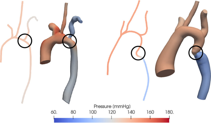
Comparison of pressure distribution estimated using $0\text{D}$ (left) and $3\text{D}$ (right) simulations in 2 representative patients with vessel narrowing at different locations - at a vessel junction and in the descending aorta. The location of the coarctation is circled in black.

Fig. 5.

Pressure over the normalized vessel path along the aorta estimated using $0\text{D}$ (dotted) and $3\text{D}$ (solid) simulations at peak systole. Results are depicted for two representative patients with CoA at different locations (red box) - at a vessel junction (top) and in the DAo (bottom). Junctions regions are depicted in pink.

The measurements of $\mathrm{\Delta }{\mathrm{P}}_{0\text{D}}$ depicted in Figure 6 show a larger deviation from $\mathrm{\Delta }{\mathrm{P}}_{\text{Cath}}$ for patients with CoA in the junction, while $\mathrm{\Delta }{\mathrm{P}}_{3\text{D}}$ matches $\mathrm{\Delta }{\mathrm{P}}_{\text{Cath}}$ very closely in most cases.

Fig. 6.

Comparison of CoA pressure drop estimated using $0\text{D}$ (left) and $3\text{D}$ (right) simulations with catheter-derived pressure measurements. Dotted line indicates no error between simulation results and catheter measurements.

The agreement between simulation and catheter-derived $\mathrm{\Delta }\mathrm{P}$ estimates was evaluated using Bland-Altman analysis shown in Figure 7. Both $\mathrm{\Delta }{\mathrm{P}}_{0\text{D}}$ and $\mathrm{\Delta }{\mathrm{P}}_{3\text{D}}$ resulted in average underestimation of $\mathrm{\Delta }{\mathrm{P}}_{\text{Cath}}$ that was larger in the case of $\mathrm{\Delta }{\mathrm{P}}_{0\text{D}}$. The bias (mean of differences) was higher for $\mathrm{\Delta }{\mathrm{P}}_{0\text{D}}$ (−7.29 mmHg) than for $\mathrm{\Delta }{\mathrm{P}}_{3\text{D}}$ (−0.76 mmHg). The corresponding limits of agreement were ± 18.08 mmHg and ± 9.39 mmHg for $\mathrm{\Delta }{\mathrm{P}}_{0\text{D}}$ and $\mathrm{\Delta }{\mathrm{P}}_{3\text{D}}$, respectively. For the cases that specifically had a “non-junction” CoA, both the $0\text{D}$ and the $3\text{D}$ simulations provided closer estimates to $\mathrm{\Delta }{\mathrm{P}}_{\text{Cath}}$ than for “junction” CoA cases. The bias of $\mathrm{\Delta }{\mathrm{P}}_{0\text{D}}$ was −3.1 ± 15.6 mmHg versus −12 ± 14.4 mmHg and for $\mathrm{\Delta }{\mathrm{P}}_{3\text{D}}$ was −0.23 ± 5.23 mmHg versus −1.88 ± 11.6 mmHg for “junction” versus “non-junction” CoA.

Fig. 7.

Bland-Altman plots of catheter-derived pressure gradient and estimates from $0\text{D}$ (left) and $3\text{D}$ (right) simulations. The solid lines represent the mean difference between simulation and catheter pressure gradient estimates, and the paired dotted lines correspond to the 95% limits of agreement.

In the clinical setting, a $\mathrm{\Delta }\mathrm{P}$ cutoff of 20 mmHg at rest across the CoA is used to guide the decision to intervene. $\mathrm{\Delta }\mathrm{P}<20\mathrm{m}\mathrm{m}\mathrm{H}\mathrm{g}$ is classified as a “mild” CoA and $\mathrm{\Delta }\mathrm{P}\ge 20\mathrm{m}\mathrm{m}\mathrm{H}\mathrm{g}$ is considered a “severe” CoA likely needing corrective intervention. Using this cutoff, $\mathrm{\Delta }{\mathrm{P}}_{0\text{D}}$ and $\mathrm{\Delta }{\mathrm{P}}_{3\text{D}}$ would result in the right treatment recommendation in 76% and 88% of cases, respectively (Figure 8). If a severe CoA is considered “positive”, the $0\text{D}$ estimate has a sensitivity of 33.3% and specificity of 100%. The $3\text{D}$ estimate has a sensitivity of 83.3% and specificity of 90.9%. In junction CoA cases, the $0\text{D}$ estimate has sensitivity and specificity of 0% and 100% respectively while the $3\text{D}$ estimate has sensitivity and specificity of 66% and 80% respectively. In non-junction CoA cases, the $0\text{D}$ estimate has sensitivity and specificity of 66% and 100% respectively while the $3\text{D}$ estimate has sensitivity and specificity of 100% and 100% respectively.

Fig. 8.

Confusion matrix for severity of CoA as determined by $\mathrm{\Delta }{\mathrm{P}}_{\text{Cath}}$ and $\mathrm{\Delta }{\mathrm{P}}_{0\text{D}}$ (left), $\mathrm{\Delta }{\mathrm{P}}_{\text{Cath}}$ and $\mathrm{\Delta }{\mathrm{P}}_{3\text{D}}$ (right). “Mild”: $\mathrm{\Delta }\mathrm{P}<20\mathrm{m}\mathrm{m}\mathrm{H}\mathrm{g}$, “Severe”: $\mathrm{\Delta }\mathrm{P}\ge 20\mathrm{m}\mathrm{m}\mathrm{H}\mathrm{g}$.

Paired Student’s t-test between $\mathrm{\Delta }{\mathrm{P}}_{0\text{D}}$ and $\mathrm{\Delta }{\mathrm{P}}_{\text{Cath}}$ had a p-value < 0.001 indicating that $\mathrm{\Delta }{\mathrm{P}}_{0\text{D}}$ was not always a good estimate of clinical catheter-derived pressures. The t-test between $\mathrm{\Delta }{\mathrm{P}}_{3\text{D}}$ and $\mathrm{\Delta }{\mathrm{P}}_{\text{Cath}}$ had p-value = 0.565, indicating that the null hypothesis was not rejected and that $\mathrm{\Delta }{\mathrm{P}}_{3\text{D}}$ provides non-invasive estimates of catheter pressures that are not significantly different.

4. Discussion

Invasive catheterization is the current gold standard for treatment decisions in patients with CoA. However, it is a costly procedure which is not risk-free, and thus there is a need for accurate non-invasive alternatives for estimation of $\mathrm{\Delta }\mathrm{P}$. This study addresses this need and validates a CFD-based method for non-invasive estimation of aortic BP gradient in patient-specific models of CoA. $0\text{D}$ models (constructed automatically from $3\text{D}$ models) were used to efficiently tune boundary conditions, to initialize $3\text{D}$ simulations, and to compute flow and pressure in patient-specific models of CoA for comparison with full fidelity simulations.

$\mathrm{\Delta }\mathrm{P}$ predicted from $0\text{D}$ and $3\text{D}$ simulation validated using invasive catheter measurements had smaller percentage errors with catheterization than Doppler and arm-leg cuff BP measurements. $3\text{D}$ models estimated $\mathrm{\Delta }\mathrm{P}$ within 5 mmHg in most cases and had an average error of 12%. The $0\text{D}$ model had an average error of 30%, but was also a good estimator of catheter-derived pressure gradients in cases where the CoA was in a non-junction region.

The significantly lower computational time of the $0\text{D}$ models make them more feasible to use in a clinical setting in scenarios where the CoA is not located at a vessel junction. While $0\text{D}$ simulations are computationally efficient, the simplified nature of these models and lack of features such as wave propagation affects their accuracy. Unsurprisingly, the results of our study confirmed that the $0\text{D}$ model is not a sufficiently accurate standalone model for estimating $\mathrm{\Delta }\mathrm{P}$ in patients with CoA. One potential source of error in $0\text{D}$ models is the automatic stenosis detection. The vessel cross-sectional areas $S_0$ and $S_s$ (3) are crucial to accurately determine the resistance in the stenosis. In our framework, $S_0$ and $S_s$ are determined automatically and can give rise to errors when comparing the results of $0\text{D}$ and $3\text{D}$ simulations. Additionally, due to the complexity of solving for pressures and flows at junctions, the current $0\text{D}$ solver implements mass conservation at junction regions and assumes the pressure is constant between the inlets and outlets of the junction. Pressure drops in a junction, which often result from nonlinear effects such as flow separation, are therefore not accurately resolved. With future improvements to $0\text{D}$ models, they have the potential to become more accurate. Therefore, while $0\text{D}$ simulations cannot currently replace $3\text{D}$ simulations, they can be used to speed up the $3\text{D}$ model personalization process. They can be used as an efficient surrogate to iteratively tune boundary conditions within a couple of minutes. $3\text{D}$ simulations initialized with $0\text{D}$ results also converge in fewer cycles than they would without any initialization, thereby decreasing the computational cost and time of running a $3\text{D}$ CFD simulation.

This study has several limitations. Patients with CoA combined with aortic valve stenosis were excluded from the study given the lack of information to recreate the spatial inflow pattern from CT images in simulations which would significantly affect $\mathrm{\Delta }\mathrm{P}$ estimates downstream. Patients who had extensive collaterals were also excluded because of the lack of image resolution to segment these small vessels and quantify flow through them. Second, the same Young’s modulus obtained from literature was used for the vessel walls for all patients in this cohort, making the CFD results prone to error in the case of a mismatch; this information is not currently available on a patient specific basis. Third, while inflow measurements from the day of the imaging exam were used to inform the models for patients with MRI, pressure estimates derived from these models were compared to pressures measured on the day of catheterization (which was on average 80 days after the MRI exam). Any differences in the patient’s hemodynamic state between the MRI exam and the catheterization procedure would therefore contribute to errors.

For patients who only had a CT, their inflow waveform was an averaged waveform scaled to match the patient’s CO and HR. The CO used for this was estimated using the Fick’s method during the catheterization procedure. Therefore, for patients with CT analysis, this study’s proposed method is not entirely non-invasive. In the future, CO measurements from echocardiography or MRI could be used to make the method completely non-invasive. The patient-specific models and simulations framework described in this study can also be extended to study the impact of exercise on hemodynamics, particularly $\mathrm{\Delta }\mathrm{P}$, in CoA patients. This metric cannot reliably be measured in the clinic. Future studies could also aim to address the inability of the $0\text{D}$ models to detect pressure drops at junctions. Machine learning models trained on hundreds of cardiovascular models in the Vascular Model Repository (vascularmodel.org) to better estimate pressure loss across junctions are currently in development and will be incorporated into subsequent iterations of the $0\text{D}$ model.

In conclusion, we have shown the capability of a combined $0\text{D}-3\text{D}$ simulation approach that accurately recapitulates invasive cardiac catheterization measurements and can guide patient-specific treatment planning in patients with CoA. Future work should assess the predictive accuracy of our methods in a prospective clinical study with a larger cohort.

Availability of data and materials:

The datasets generated during this study will be available in the Vascular Model Repository (vascularmodel.org).

References

- [1].Singh S., Hakim F.A., Sharma A., Roy R.R., Panse P.M., Chandrasekaran K., Alegria J.R., Mookadam F.: Hypoplasia, pseudocoarctation and coarctation of the aorta–a systematic review. Heart, Lung and Circulation 24(2), 110–118 (2015) 10.1016/j.hlc.2014.08.006 [DOI] [PubMed] [Google Scholar]
- [2].Torok R.D., Campbell M.J., Fleming G.A., Hill K.D.: Coarctation of the aorta: Management from infancy to adulthood. World journal of cardiology 7(11), 765–775 (2015) 10.4330/wjc.v7.i11.765 [DOI] [PMC free article] [PubMed] [Google Scholar]
- [3].Bashore T.M., Child J.S., Connolly H.M., Dearani J.A., Nido P., Fasules J.W., Graham T.P., Hijazi Z.M., Hunt S.A., Etta King M., Landzberg M.J., Miner P.D., Radford M.J., Walsh E.P., Webb G.D., Adams C.D., Anderson J.L., Antman E.M., Buller C.E., Creager M.A., Ettinger S.M., Halperin J.L., Krumholz H.M., Kushner F.G., Lytle B.W., Nishimura R.A., Page R.L., Riegel B., Tarkington L.G., Yancy C.W.: ACC/AHA 2008 Guidelines for the Management of Adults With Congenital Heart Disease. Circulation 118(23), 714–833 (2008) 10.1161/CIRCULATIONAHA.108.190690 [DOI] [PubMed] [Google Scholar]
- [4].Jenkins N.P., Ward C.: Coarctation of the aorta: natural history and outcome after surgical treatment. Qjm 92(7), 365–371 (1999) 10.1093/qjmed/92.7.365 [DOI] [PubMed] [Google Scholar]
- [5].Therrien J., Warnes C., Daliento L., Hess J., Hoffmann A., Marelli A., Thilen U., Presbitero P., Perloff J., Somerville J., Webb G.D.: Canadian Cardiovascular Society Consensus Conference 2001 update: recommendations for the management of adults with congenital heart disease part III. The Canadian journal of cardiology 17(11), 1135–1158 (2001) [PubMed] [Google Scholar]
- [6].Seifert B.L., DesRochers K., Ta M., Giraud G., Zarandi M., Gharib M., Sahn D.J.: Accuracy of Doppler methods for estimating peak-to-peak and peak instantaneous gradients across coarctation of the aorta: an in vitro study. Journal of the American Society of Echocardiography 12(9), 744–753 (1999) 10.1016/s0894-7317(99)70025-8 [DOI] [PubMed] [Google Scholar]
- [7].Itu L., Sharma P., Ralovich K., Mihalef V., Ionasec R., Everett A., Ringel R., Kamen A., Comaniciu D.: Non-Invasive Hemodynamic Assessment of Aortic Coarctation: Validation with In Vivo Measurements. Annals of Biomedical Engineering 41(4), 669–681 (2013) 10.1007/s10439-012-0715-0 [DOI] [PubMed] [Google Scholar]
- [8].Grande Gutierrez N., Mathew M., McCrindle B.W., Tran J.S., Kahn A.M., Burns J.C., Marsden A.L.: Hemodynamic variables in aneurysms are associated with thrombotic risk in children with Kawasaki disease. International Journal of Cardiology 281, 15–21 (2019) 10.1016/j.ijcard.2019.01.092 [DOI] [PMC free article] [PubMed] [Google Scholar]
- [9].Marsden A.L., Bernstein A.J., Reddy V.M., Shadden S.C., Spilker R.L., Chan F.P., Taylor C.A., Feinstein J.A.: Evaluation of a novel Y-shaped extracardiac Fontan baffle using computational fluid dynamics. The Journal of Thoracic and Cardiovascular Surgery 137(2), 394–403 (2009) 10.1016/j.jtcvs.2008.06.043 [DOI] [PubMed] [Google Scholar]
- [10].Kwon S., Feinstein J.A., Dholakia R.J., LaDisa J.F.: Quantification of local hemodynamic alterations caused by virtual implantation of three commercially available stents for the treatment of aortic coarctation. Pediatric cardiology 35, 732–740 (2014) 10.1007/s00246-013-0845-7 [DOI] [PMC free article] [PubMed] [Google Scholar]
- [11].Wei Z.A., Johnson C., Trusty P., Stephens M., Wu W., Sharon R., Srimurugan B., Kottayil B.P., Sunil G.S., Fogel M.A.: Comparison of Fontan surgical options for patients with apicocaval juxtaposition. Pediatric cardiology 41, 1021–1030 (2020) 10.1007/s00246-020-02353-8 [DOI] [PMC free article] [PubMed] [Google Scholar]
- [12].Celestin C., Guillot M., Ross-Ascuitto N., Ascuitto R.: Computational fluid dynamics characterization of blood flow in central aorta to pulmonary artery connections: importance of shunt angulation as a determinant of shear stress-induced thrombosis. Pediatric cardiology 36, 600–615 (2015) 10.1007/s00246-014-1055-7 [DOI] [PubMed] [Google Scholar]
- [13].Saitta S., Pirola S., Piatti F., Votta E., Lucherini F., Pluchinotta F., Carminati M., Lombardi M., Geppert C., Cuomo F., Figueroa C.A., Xu X.Y., Redaelli A.: Evaluation of 4D flow MRI-based non-invasive pressure assessment in aortic coarctations. Journal of biomechanics 94, 13–21 (2019) 10.1016/j.jbiomech.2019.07.004 [DOI] [PubMed] [Google Scholar]
- [14].Aslan S., Mass P., Loke Y.-H., Warburton L., Liu X., Hibino N., Olivieri L., Krieger A.: Non-invasive Prediction of Peak Systolic Pressure Drop across Coarctation of Aorta using Computational Fluid Dynamics. Annual International Conference of the IEEE Engineering in Medicine and Biology Society. IEEE Engineering in Medicine and Biology Society. Annual International Conference 2020, 2295–2298 (2020) 10.1109/EMBC44109.2020.9176461 [DOI] [PMC free article] [PubMed] [Google Scholar]
- [15].Ladisa J.F., Alberto Figueroa C., Vignon-Clementel I.E., Jin Kim H., Xiao N., Ellwein L.M., Chan F.P., Feinstein J.A., Taylor C.A.: Computational simulations for aortic coarctation: Representative results from a sampling of patients. Journal of Biomechanical Engineering 133(9) (2011) 10.1115/1.4004996 [DOI] [PMC free article] [PubMed] [Google Scholar]
- [16].O’ROURKE M.F., CARTMILL T.B.: Influence of aortic coarctation on pulsatile hemodynamics in the proximal aorta. Circulation 44(2), 281–292 (1971) 10.1161/01.cir.44.2.281 [DOI] [PubMed] [Google Scholar]
- [17].Shahid L., Rice J., Berhane H., Rigsby C., Robinson J., Griffin L., Markl M., Roldán-Alzate A.: Enhanced 4D flow MRI-based CFD with adaptive mesh refinement for flow dynamics assessment in coarctation of the aorta. Annals of Biomedical Engineering 50(8), 1001–1016 (2022) 10.1007/s10439-022-02980-7 [DOI] [PMC free article] [PubMed] [Google Scholar]
- [18].Goubergrits L., Riesenkampff E.Cardiovascular engineering and technology, Yevtushenko P., Schaller J., Kertzscher U., Hennemuth A., Berger F., Schubert S., Kuehne T.: MRI-based computational fluid dynamics for diagnosis and treatment prediction: Clinical validation study in patients with coarctation of aorta. Journal of Magnetic Resonance Imaging 41(4), 909–916 (2015) 10.1002/jmri.24639 [DOI] [PubMed] [Google Scholar]
- [19].Brüning J., Hellmeier F., Yevtushenko P., Kühne T., Goubergrits L.: Uncertainty quantification for non-invasive assessment of pressure drop across a coarctation of the aorta using CFD. Cardiovascular engineering and technology 9, 582–596 (2018) 10.1007/s13239-018-00381-3 [DOI] [PubMed] [Google Scholar]
- [20].Perktold K., Rappitsch G.: Computer simulation of local blood flow and vessel mechanics in a compliant carotid artery bifurcation model. Journal of biomechanics 28(7), 845–856 (1995) 10.1016/0021-9290(95)95273-8 [DOI] [PubMed] [Google Scholar]
- [21].Formaggia L., Gerbeau J.-F., Nobile F., Quarteroni A.: On the coupling of and 1D Navier–Stokes equations for flow problems in compliant vessels. Computer methods in applied mechanics and engineering 191(6–7), 561–582 (2001) 10.1016/S0045-7825(01)00302-4 [DOI] [Google Scholar]
- [22].Vignon-Clementel I.E., Figueroa C.A., Jansen K.E., Taylor C.A.: Outflow boundary conditions for three-dimensional finite element modeling of blood flow and pressure in arteries. Computer methods in applied mechanics and engineering 195(29–32), 3776–3796 (2006) 10.1016/j.cma.2005.04.014Getrightsandcontent [DOI] [Google Scholar]
- [23].Pfaller M.R., Pham J., Verma A., Pegolotti L., Wilson N.M., Parker D.W., Yang W., Marsden A.L.: Automated generation of 0D and 1D reduced-order models of patient-specific blood flow. International Journal for Numerical Methods in Biomedical Engineering 38(10), 3639 (2022) 10.1002/cnm.3639 [DOI] [PMC free article] [PubMed] [Google Scholar]
- [24].Updegrove A., Wilson N.M., Merkow J., Lan H., Marsden A.L., Shadden S.C.: SimVascular: An Open Source Pipeline for Cardiovascular Simulation. Annals of Biomedical Engineering 45(3), 525–541 (2017) 10.1007/s10439-016-1762-8 [DOI] [PMC free article] [PubMed] [Google Scholar]
- [25].Mirramezani M., Shadden S.C.: A Distributed Lumped Parameter Model of Blood Flow. Annals of Biomedical Engineering 48(12), 2870–2886 (2020) 10.1007/s10439-020-02545-6 [DOI] [PMC free article] [PubMed] [Google Scholar]
- [26].Mirramezani M., Diamond S.L., Litt H.I., Shadden S.C.: Reduced order models for transstenotic pressure drop in the coronary arteries. Journal of biomechanical engineering 141(3), 031005 (2019) 10.1115/1.4042184 [DOI] [PMC free article] [PubMed] [Google Scholar]
- [27].Steele B.N., Wan J., Ku J.P., Hughes T.J.R., Taylor C.A.: In vivo validation of a one-dimensional finite-element method for predicting blood flow in cardiovascular bypass grafts. IEEE Transactions on Biomedical Engineering 50(6), 649–656 (2003) 10.1109/TBME.2003.812201 [DOI] [PubMed] [Google Scholar]
- [28].Pfaller M.R., Pham J., Wilson N.M., Parker D.W., Marsden A.L.: On the Periodicity of Cardiovascular Fluid Dynamics Simulations. Annals of Biomedical Engineering 49(12), 3574–3592 (2021) 10.1007/s10439-021-02796-x [DOI] [PMC free article] [PubMed] [Google Scholar]
- [29].Figueroa C.A., Vignon-Clementel I.E., Jansen K.E., Hughes T.J.R., Taylor C.A.: A coupled momentum method for modeling blood flow in three-dimensional deformable arteries. Computer methods in applied mechanics and engineering 195(41–43), 5685–5706 (2006) 10.1016/j.cma.2005.11.011 [DOI] [Google Scholar]
- [30].Filonova V., Arthurs C.J., Vignon-Clementel I.E., Figueroa C.A.: Verification of the coupled-momentum method with Womersley’s Deformable Wall analytical solution. International journal for numerical methods in biomedical engineering 36(2), 3266 (2020) 10.1002/cnm.3266 [DOI] [PMC free article] [PubMed] [Google Scholar]
- [31].Lan I.S., Liu J., Yang W., Zimmermann J., Ennis D.B., Marsden A.L.: Validation of the Reduced Unified Continuum Formulation Against In Vitro 4D-Flow MRI. Annals of Biomedical Engineering 51(2), 377–393 (2023) 10.1007/s10439-022-03038-4 [DOI] [PMC free article] [PubMed] [Google Scholar]
Associated Data
This section collects any data citations, data availability statements, or supplementary materials included in this article.
Data Availability Statement