Air pollution exposure disparities across US population and income groups

Summary Paragraph

Air pollution contributes to the global burden of disease, with ambient exposure to fine particulate matter with diameter smaller than 2.5 micrometres (${\mathrm{P}\mathrm{M}}_{2.5}$) identified as the fifth-ranking risk factor of mortality globally [1]. Racial/ethnic minorities and lower income groups in the USA are at a higher risk of death from exposure to ${\mathrm{P}\mathrm{M}}_{2.5}$ [2–5]. Disparities in air pollution exposure among population and income groups are known to exist [6–17]. We develop a data platform that links demographic data (from US Census bureau and American Community Survey) and ${\mathrm{P}\mathrm{M}}_{2.5}$ data [18] across the USA. We analyse the data at the US zip code tabulation area level (N≈32000) between 2000 and 2016. We show that areas with higher than average white and Native American populations have been consistently exposed to average ${\mathrm{P}\mathrm{M}}_{2.5}$ levels lower than areas with higher than average Black, Asian and Hispanic or Latino populations. Areas with low-income groups have been consistently exposed to higher average ${\mathrm{P}\mathrm{M}}_{2.5}$ levels than areas with high-income groups for the years 2004–2016. Further, disparities in exposure relative to safety standards set by the US Environmental Protection Agency [19] and the World Health Organization [20] have been increasing over time. This suggests that more targeted ${\mathrm{P}\mathrm{M}}_{2.5}$ reductions are necessary to provide all people with similar degree of protection from environmental hazards. Our study is observational and cannot provide insight into the drivers of the identified disparities.

Several studies have reported evidence of statistically significant associations between exposure to ${\mathrm{P}\mathrm{M}}_{2.5}$ (fine particles with a mass median aerodynamic diameter of less than 2.5 μm) and adverse health outcomes [21–34], and it is well documented that racial-ethnic minorities and people of low socioeconomic status in the US are at a higher risk of death from being exposed to ${\mathrm{P}\mathrm{M}}_{2.5}$ [2–5]. Disparities in air pollution exposure among racial/ethnic and socioeconomic groups in the US are also known to exist [6–15]. Disparities may be represented as either relative or absolute comparisons, where absolute disparities are assessed as absolute differences between groups, while relative disparities are scale invariant [16]. A recent study showed that absolute disparities in ${\mathrm{P}\mathrm{M}}_{2.5}$ between more and less polluted areas in the US have declined substantially between 1981 and 2001 but that relative disparities persist [17].

In this paper, we advance this line of work by studying relative disparities across income groups (namely income deciles) and racial/ethnic groups for the years 2000 to 2016. Here, ethnic groups are defined as those with shared cultural characteristics and racial groups as those with physical differences that they consider to be socially significant [35]. The ethnic group included in this study is the Hispanic or Latino group, and the racial groups are white, Black, Asian and Native American; for ease of reference, the racial groups are referred to as white, Black, Asian and Native American throughout the text. Further, we stress that the present study is descriptive and is not designed to investigate causal aspects related to race. Further novelty of our study includes the investigation of relative disparities relative to safety standards (National Ambient Air Quality standard (NAAQS) set by the US Environmental Protection Agency (EPA) at 12 μg/m³ [19], and the guideline set by the World Health Organization (WHO) at 10 μg/m³ [20]) and their trends over the study period.

Our study’s findings on relative disparities indicate the importance of strong targeted air-pollution reduction strategies to not only reduce overall air pollution levels but also to move closer towards EPA’s aim to provide all people the same degree of protection from environmental hazards. Nonetheless, the presented evidence should be interpreted in the context of the limitations of the data at hand. Mainly, the ${\mathrm{P}\mathrm{M}}_{2.5}$ concentrations used in this study rely on aerosol optical depth (AOD) data (see Methods section). AOD-based particulate estimates tend to underestimate pollution at higher levels and overestimate it at very low levels. In addition, US Census data is used and is not available for every year of the study period (see Methods section), so we have used interpolation techniques for parts of the study period and hence our results are subject to the assumptions made in the interpolation. Finally, average ${\mathrm{P}\mathrm{M}}_{2.5}$ concentrations across ZCTAs are used, which can mask the relationship between income and pollution levels of neighborhoods within large ZCTAs, and are subject to more error in cases where substantial within-ZCTA variation in pollution occurs.

Disparities among racial/ethnic groups

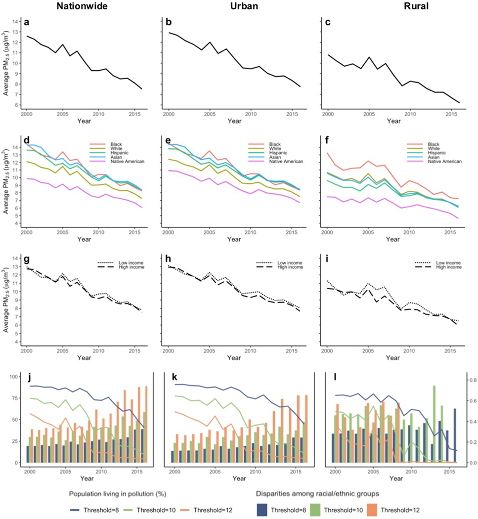
The US EPA is required to reexamine the NAAQS every five years. In 2012, the EPA set the NAAQS for ${\mathrm{P}\mathrm{M}}_{2.5}$ to 12 μg/m³ [19, 36]. On average across the US, we found that ${\mathrm{P}\mathrm{M}}_{2.5}$ concentration levels decreased from 2000 to 2016, where the population-weighted average of ${\mathrm{P}\mathrm{M}}_{2.5}$ has decreased by 40% from the year 2000 (12.6 μg/m³) to 2016 (7.5 μg/m³). (video 1 in supplementary material; and Extended Data figure A.1a). We also found that the percentage of the population exposed to ${\mathrm{P}\mathrm{M}}_{2.5}$ levels higher than 12 μg/m³ decreased from 57.3% in 2000 to 4.5% in 2016.

Next, we visualize and examine disparities in air pollution exposure among racial/ethnic groups. For each racial/ethnic group (white, Black, Asian, Native American and Hispanic or Latino), we construct a map that shows zip code tabulation areas (ZCTAs) where the race/ethnicity is overrepresented. In the case of the white population for example, we use the white population fraction of the ZCTA population to compute the average white population fraction across all ZCTAs (≈ 84.2%). We then set the margin at 84% and only show on the map ZCTAs with a white population fraction exceeding this margin. The margins for the remaining racial/ethnics groups were computed similarly and are shown in Extended Data Figure A.3. For ease of exposition, we present findings for only two groups in the main text (white and Black groups in figure 1) and include the other racial/ethnic groups in Extended Data Figure A.3 and videos 2 and 3. Figures 1a and 1b show the ${\mathrm{P}\mathrm{M}}_{2.5}$ distributions in ZCTAs where the Black and white populations are overrepresented for the years 2000 and 2016, respectively. We found that ZCTAs where the Black population is overrepresented (left map) are dominated by high ${\mathrm{P}\mathrm{M}}_{2.5}$ concentrations relative to those ZCTAs with white overrepresentation (right map) in both 2000 and 2016. Furthermore, we see a steeper decline in ${\mathrm{P}\mathrm{M}}_{2.5}$ among the latter.

Figure 1. Average ${\mathrm{P}\mathrm{M}}_{2.5}$ concentration in 2000 and 2016 across ZCTAs where Black and white populations are overrepresented:

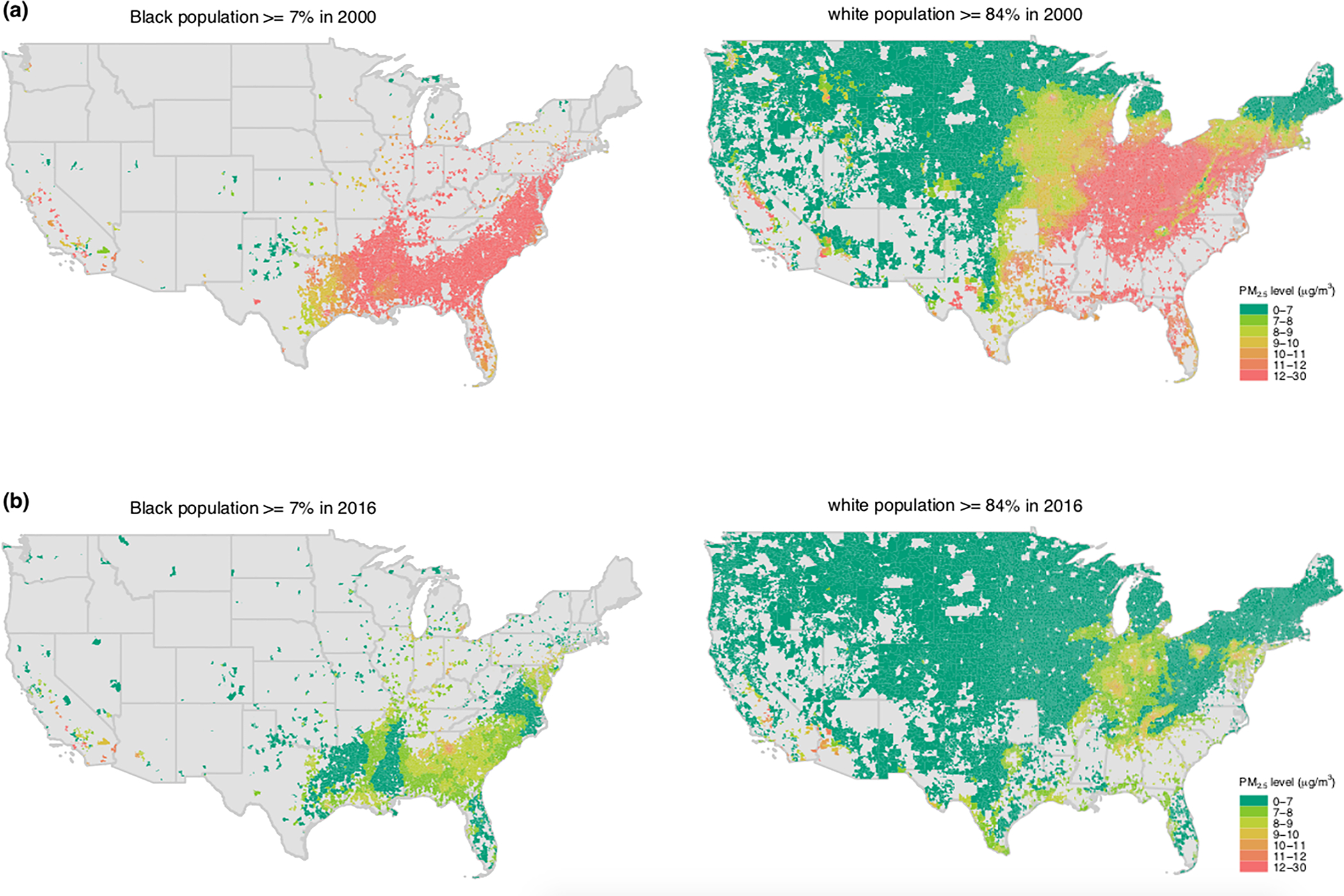
We use the white population fraction of the ZCTA population to compute the average white population fraction (aWpf) across all ZCTAs (≈ 84%). Similarly, we compute the average Black population fraction (aBpf) (≈ 7%). The maps in panel (a) show ${\mathrm{P}\mathrm{M}}_{2.5}$ levels for the year 2000 in ZCTAs with a Black population fraction above aBpf (left) and in ZCTAs with a white population fraction above aWpf (right). High ${\mathrm{P}\mathrm{M}}_{2.5}$ concentrations exist in almost all ZCTAs with a Black population above aBpf, while a wide range of low and high ${\mathrm{P}\mathrm{M}}_{2.5}$ concentrations exist in ZCTAs with a white population above aWpf in 2000. Panel (b) shows the same information for the year 2016. Similar maps for the other racial/ethnic groups for 2000 and 2016 are shown in Extended Data figures 1.a and 1.b and videos 2 and 3 in supplementary material.

We also compute the population-weighted average ${\mathrm{P}\mathrm{M}}_{2.5}$ concentration for every racial/ethnic population (please see Methods) (Extended Data figure A.1b). For all years, we found that the Black, Asian and Hispanic or Latino populations experience somewhat similar levels of ${\mathrm{P}\mathrm{M}}_{2.5}$ that are higher than those experienced by the white population. In 2016 for example, the average ${\mathrm{P}\mathrm{M}}_{2.5}$ concentration for the Black population was 13.7% higher than that of the white population and 36.3% higher than that of the Native American population. The Native American population was consistently exposed to the lowest levels of ${\mathrm{P}\mathrm{M}}_{2.5}$. Further, we illustrate for the year 2016 how the population-weighted ${\mathrm{P}\mathrm{M}}_{2.5}$ average concentration changes as ZCTAs become more populated by a certain race/ethnicity (Extended Data figure A.1c). We found that as the Black population increases in a ZCTA, the ${\mathrm{P}\mathrm{M}}_{2.5}$ concentration consistently increases with a steep incline seen for ZCTAs with more than 85% of their population as Black. The trend for the Hispanic or Latino population is similar to that of the Black population. The opposite is seen for the white population; ${\mathrm{P}\mathrm{M}}_{2.5}$ concentration decreases as density of the white population increases in ZCTAs; a steeper decrease is shown for ZCTAs with a white population fraction exceeding 70%. Further, in ZCTAs where the population of Native Americans is at least 20%, the average ${\mathrm{P}\mathrm{M}}_{2.5}$ concentration drops to below 4 μg/m³. For the Asian population, a very low number of ZCTAs has a population density above 60%, so data beyond this point is not representative and not shown.

Disparities among income groups

We next visualize and summarize disparities among income groups. We assign all ZCTAs percentile ranks from 1 to 100 based on median household income and categorize them into ten income groups. We designate the lowest and highest three income groups as low-income and high-income respectively and then split the US map into two maps – ZCTAs defined as low- and high-income (please see Methods). We visualize the ${\mathrm{P}\mathrm{M}}_{2.5}$ concentration distribution on the two maps for 2000 to 2016 (video 4 in supplementary material). The map with low-income ZCTAs appears visually to be dominated by an overall higher concentration of ${\mathrm{P}\mathrm{M}}_{2.5}$ as compared to the map with high-income ZCTAs especially in recent years. We include snapshots of 2000 and 2016 (figure 2). We summarize the contents of the maps by computing the population-weighted mean of ${\mathrm{P}\mathrm{M}}_{2.5}$ concentration in ZCTAs with the low- and high-income groups (Extended Data figure A.1d); ZCTAs with the low-income group are exposed to only slightly higher ${\mathrm{P}\mathrm{M}}_{2.5}$ concentrations for the majority of the study period (2004–2016); for example only 4% higher in 2016. Further, we isolate the effects of income on the disparities among the racial/ethnic groups in Extended Data figures A.1e and A.1f. For the low and high income groups, the ${\mathrm{P}\mathrm{M}}_{2.5}$ concentration differences across racial/ethnic groups are similar to those of Extended Data figure A.1b.

Figure 2. Average ${\mathrm{P}\mathrm{M}}_{2.5}$ concentration in 2000 and 2016 across low- and high-income ZCTAs:

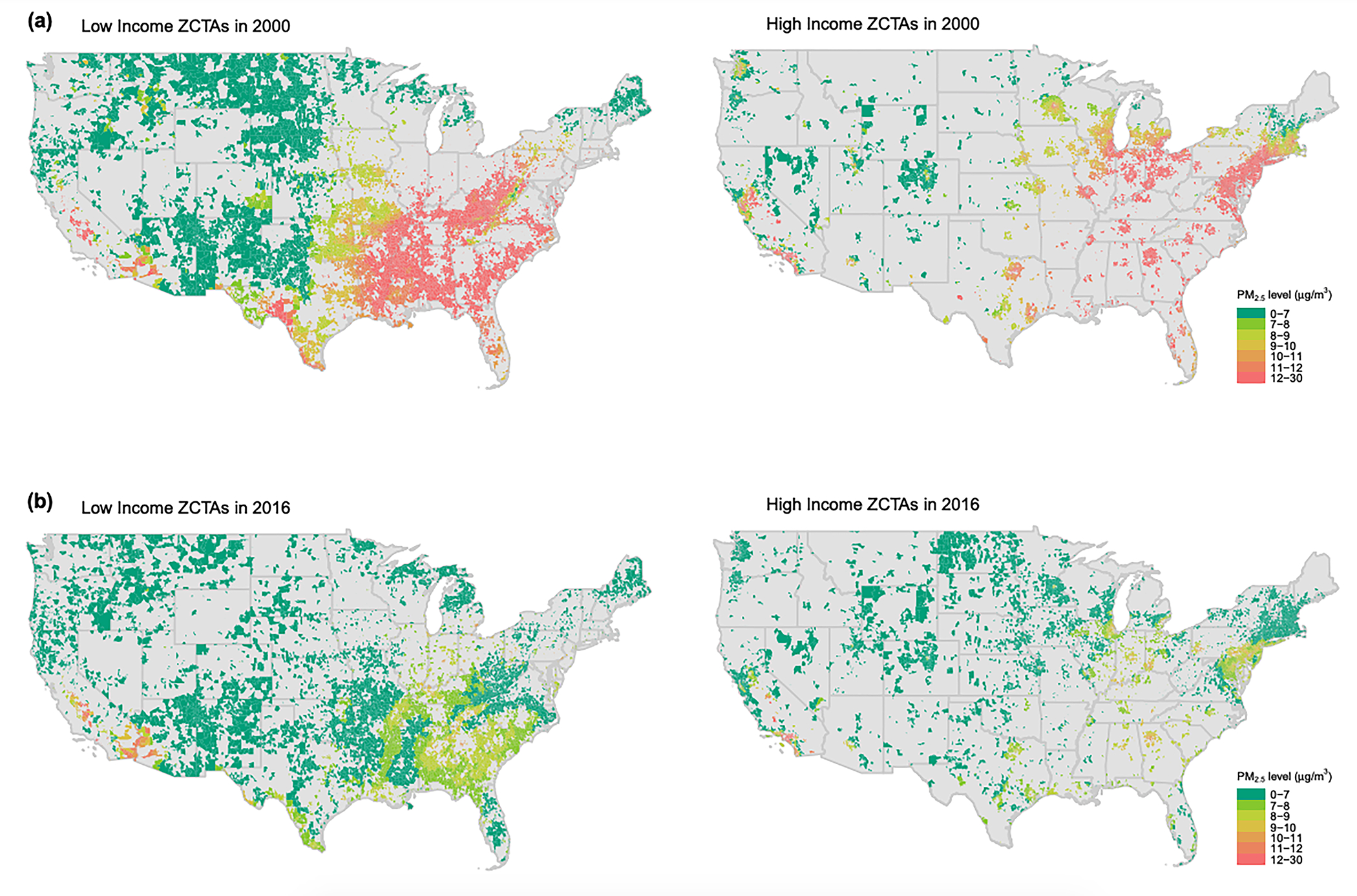
We assign all ZCTAs percentile ranks from 1 to 100 based on median household income and categorize them into ten income groups. We designate the lowest and highest three income groups as low-income and high-income respectively. The maps in panel (a) show ${\mathrm{P}\mathrm{M}}_{2.5}$ levels for the year 2000 in low-income (left) and high-income (right) ZCTAs. Panel (b) shows the same information for the year 2016. Disparities in exposure to ${\mathrm{P}\mathrm{M}}_{2.5}$ among the two groups are apparent and it can be visually seen that in both 2000 and 2016, low-income ZCTAs are exposed to higher ${\mathrm{P}\mathrm{M}}_{2.5}$ concentrations as compared to high-income ZCTAs (video 4 in supplementary material).

Disparities relative to policy standards

We investigate relative disparities in ${\mathrm{P}\mathrm{M}}_{2.5}$ exposure in the context of the current NAAQS (12 μg/m³), the guideline set by the WHO (10 μg/m³), and a lower one that may potentially be considered in the future (8 μg/m³). To do so, we estimate across the study period the proportion of every racial/ethnic group that is exposed to ${\mathrm{P}\mathrm{M}}_{2.5}$ levels higher than one of the listed safety standards. A state of equality (or lack of relative disparities) among various populations is defined as a state of equal proportions above the chosen safety standard across groups.

First, we rank the US ZCTAs from the least to the most dense with respect to every racial/ethnic group for each year. For the Black population for example, we use the Black population fraction in every ZCTA to split ZCTAs into 100 quantiles (Extended Data figure A.4a). The dark blue region on the map representing the ZCTA ranking for the Black population contains the ZCTAs with the highest ratio of Black population to total ZCTA population, and the light yellow region contains the ZCTAs with the lowest ratio of Black population to total ZCTA population. Similarly for the remaining populations, the dark blue and light yellow regions on their corresponding maps respectively signify high and low proportions of that racial/ethnic group. In figure 3a, we again focus on two groups for ease of exposition (Black and white groups are chosen for consistency). We show in the figure the ZCTAs with a ${\mathrm{P}\mathrm{M}}_{2.5}$ concentration higher than a threshold of 8 μg/m³ for the year 2000. This figure reveals that almost half of the ZCTAs with ${\mathrm{P}\mathrm{M}}_{2.5}$ concentrations above 8 μg/m³ are where the Black population is concentrated (southern part of the map as indicated by the dark blue region on the Black population US map), and the other half is where the white population is concentrated (northern part of the map as indicated by the dark blue region on the white population US map). We reproduce the same scenario for 2016 (figure 3b) and we find that the majority of ZCTAs still above 8 μg/m³ are those with concentrated Black population (majority of 2016 map representing the Black population (left) is dark blue and the majority of that representing the white population map (right) is light yellow). This visualization shows that ${\mathrm{P}\mathrm{M}}_{2.5}$ reductions between 2000 and 2016 have not benefited all areas of the US equally and consequently resulted in an increase in relative disparities to air pollution exposure as will be numerically shown later. Additionally, we extend figure 3 to include the Asian, Native American and Hispanic or Latino populations and present the results in Extended Data figures A.4. Here, we used a threshold of 8 μg/m³ for a clearer visualization of the disparities. A lower number of ZCTAs is exposed to ${\mathrm{P}\mathrm{M}}_{2.5}$ concentrations above 10 and 12 μg/m³, so visualizations at these thresholds are not as clear. Nevertheless, the same visualization is repeated for multiple thresholds including 10 and 12 μg/m³ in videos 5–8 in Supplementary Material.

Figure 3. US ZCTAs with average ${\mathrm{P}\mathrm{M}}_{2.5}$ concentration above 8 μg/m³ for the Black and white populations in 2000 and 2016:

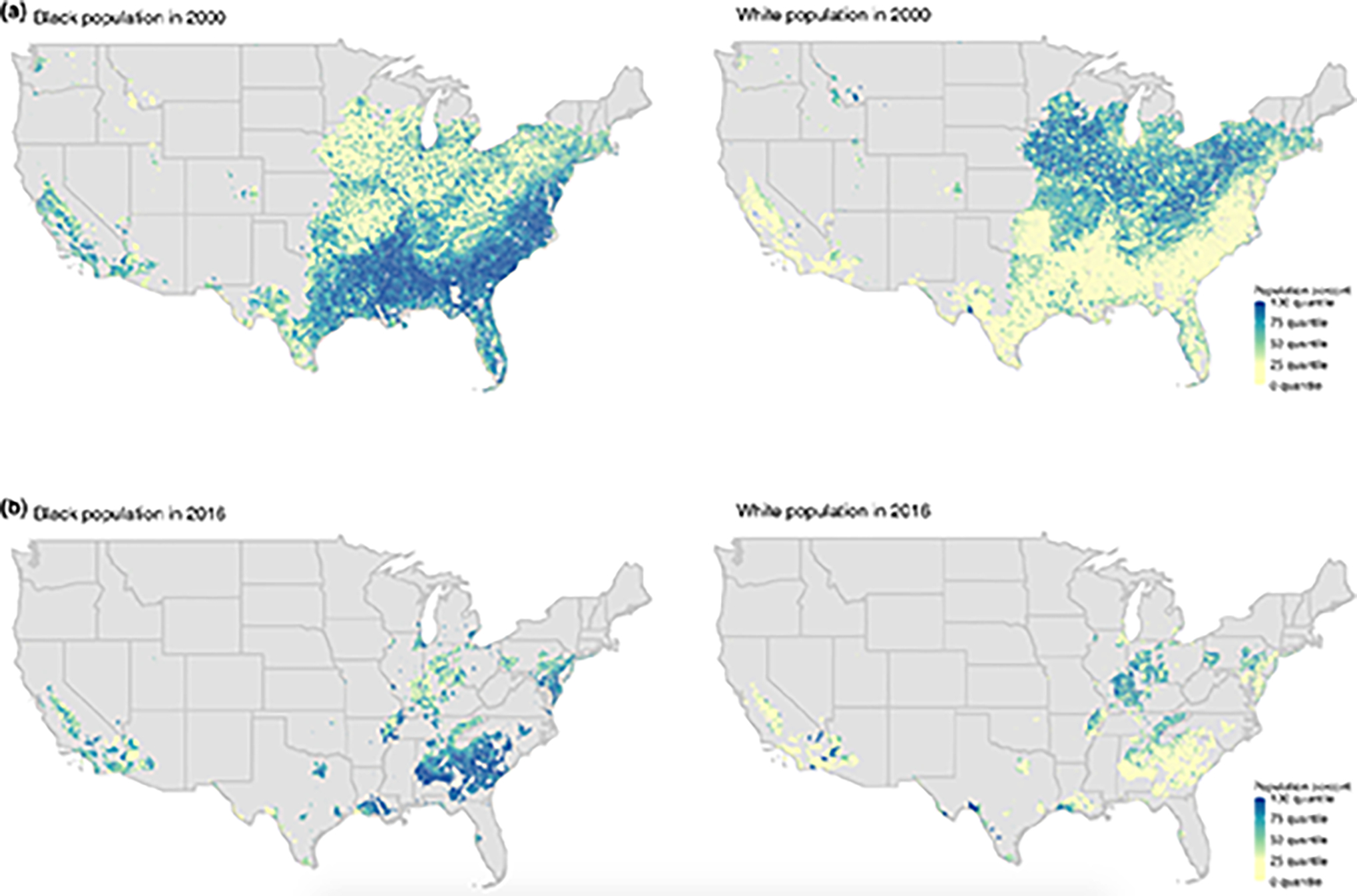
The maps only show US ZCTAs with ${\mathrm{P}\mathrm{M}}_{2.5}$ levels above 8 μg/m³ in (a) 2000 and (b) 2016. The maps on the left are color-coded based on the fraction of the Black population in ZCTAs, while the maps on the right are color-coded based on the white population fraction. For example on the left map in panel (a), the dark-blue and light-yellow colors correspond to ZCTAs with the largest and smallest Black population percentages of the total ZCTA population respectively in 2000, or equivalently where the Black population is over- and under-represented respectively in 2000. The left map of (a) reveals that almost half of the ZCTAs with ${\mathrm{P}\mathrm{M}}_{2.5}$ levels above 8 μg/m³ in 2000 correspond to those where the Black population most lives (almost half of the map is dark-blue). However in 2016, ZCTAs that remained above 8 μg/m³ are only those that are dominated by the Black population (left map in panel b). In contrast, ZCTAs that still had ${\mathrm{P}\mathrm{M}}_{2.5}$ above 8 μg/m³ in 2016 are mainly those where the white population is under-represented (right map in panel b). Videos 5–8 show the distribution of the different racial/ethnic groups across multiple ranges of ${\mathrm{P}\mathrm{M}}_{2.5}$ concentrations in 2000 and 2016 respectively.

Second, we provide numerical summaries of disparities in the proportions of racial/ethnics groups exposed to ${\mathrm{P}\mathrm{M}}_{2.5}$ levels above the chosen standard by using the coefficient of variation CoV (please see Methods) and present our findings in figure 4. Figure 4 shows that 89% of the population was exposed to ${\mathrm{P}\mathrm{M}}_{2.5}$ levels higher than 8 μg/m³ in 2000, whereas only 41% in 2016 respectively (solid blue line). However, figure 4 also reveals that relative disparities in exposure to ${\mathrm{P}\mathrm{M}}_{2.5}$ levels higher than 8 μg/m³ among racial/ethnic groups (solid blue bars) have increased from 2000 to 2016. Such result is in agreement with the relative reductions shown in figure 3. Figure 4 also shows the analysis for the thresholds $T=10\mu \mathrm{g}/m^3$ and $T=12\mu \mathrm{g}/m^3$. A consistent trend in disparities over time is seen across the different thresholds. Additionally, as expected from our definition of relative disparities, as the set threshold increases, relative differences across racial/ethnic groups become more pertinent for a given year. In addition to using the easily interpretable CoV, we repeated the disparities analysis of figure 4 using the Atkinson and Gini indices, alternative metrics used in the literature [7, 37, 38]. These findings are located in Extended Data figure A.5 and are similar to those of figure 4.

Figure 4. Relative disparities in exposure to ${\mathrm{P}\mathrm{M}}_{2.5}$ among racial/ethnic groups (Black, white, Asian, Native American and Hispanic or Latino) from 2000 to 2016:

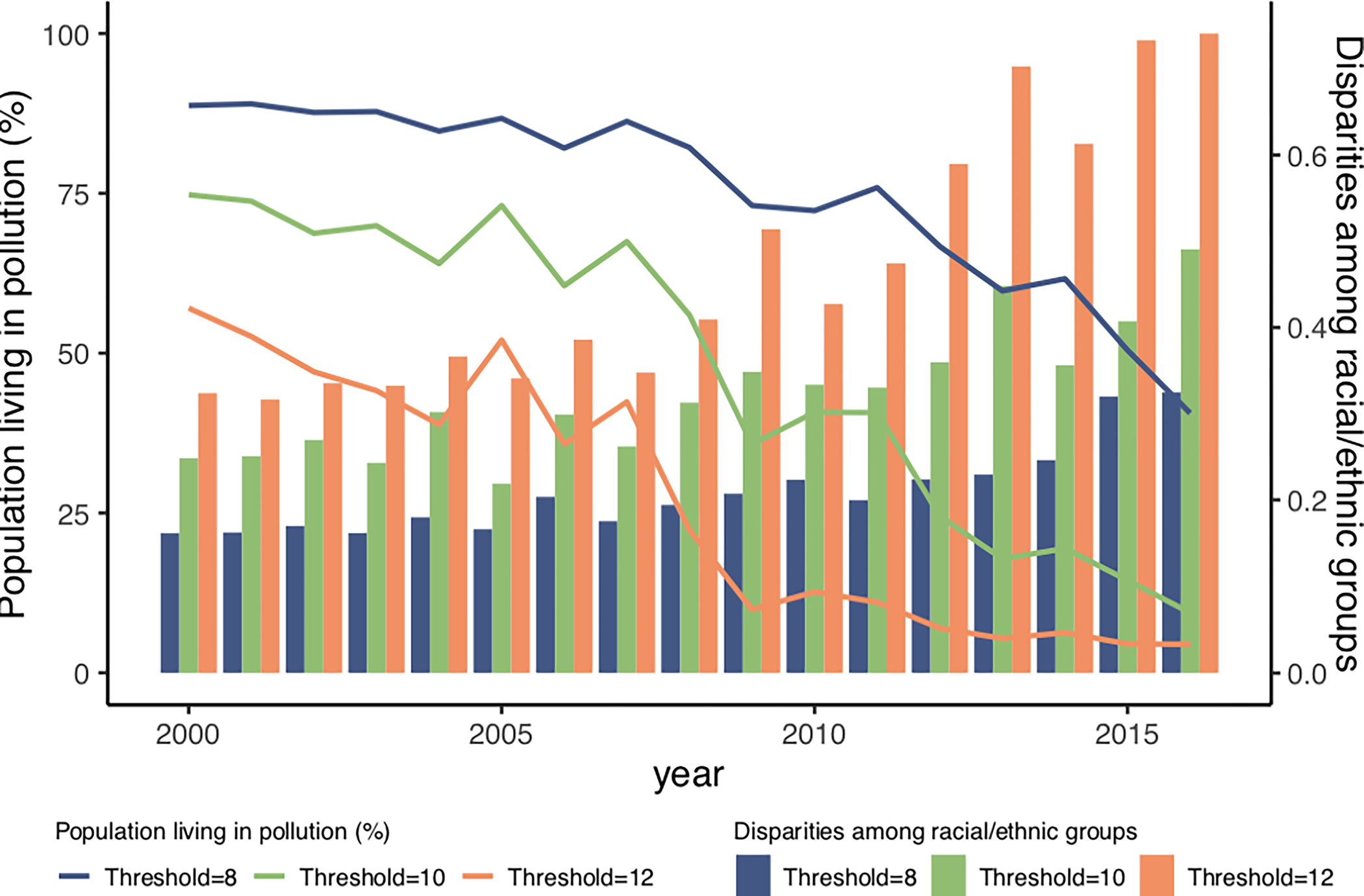
Disparities in exposure (as measured by CoV) to ${\mathrm{P}\mathrm{M}}_{2.5}$ concentrations above thresholds of 8, 10 and 12 μg/m³ for 2000 to 2016 among racial/ethnic groups (Black, white, Asian, Native American and Hispanic or Latino). The percentage of the US population living above the thresholds of 8, 10 and 12 μg/m³ is also shown. The trend reveals that the decrease in air pollution across the years has been accompanied by an increase in the relative disparities in exposure to air pollution among communities.

Discussion

We built a dataset that includes around 32 thousand US ZCTAs with detailed information on demographic and pollution data for the period 2000 to 2016. Our study provides a transparent and reproducible data science perspective and unique visualizations of the exposure to ${\mathrm{P}\mathrm{M}}_{2.5}$ in the US and the associated disparities among racial/ethnic and income groups. Our study is descriptive in nature and is not meant to investigate causal aspects of ${\mathrm{P}\mathrm{M}}_{2.5}$ reductions and disparities in the US. When possible, we have applied sensitivity analyses to confirm our findings. For example, our results were consistent across both urban and rural areas of the US (Extended Data figure A.7). In addition, we applied our analyses to two independent datasets of predicted ${\mathrm{P}\mathrm{M}}_{2.5}$ levels for the US, and our findings were consistent (Extended Data Figure A.8). Nonetheless, our study could be strengthened by addressing some caveats.

First, average ${\mathrm{P}\mathrm{M}}_{2.5}$ concentrations across ZCTAs were used. This is an important limitation because there could be substantial within-ZCTA variation in pollution. A smaller unit of analysis such as a Census block group may have further strengthened our findings, but at the cost of higher uncertainty in the estimated levels of ${\mathrm{P}\mathrm{M}}_{2.5}$ for this smaller spatial scale. Also, ${\mathrm{P}\mathrm{M}}_{2.5}$ concentrations rely on AOD estimates and are therefore subject to error. The authors [18] evaluated the performance of their approach and reported that the estimated ${\mathrm{P}\mathrm{M}}_{2.5}$ were generally consistent with direct ground-based ${\mathrm{P}\mathrm{M}}_{2.5}$. Still, it is important to interpret these values with caution. Second, the US Census data used in this study spans the years 2000 to 2016 where changes in the US population structure may have occurred. In addition to changes in pollution levels, demographic changes may have contributed to the findings presented in this paper. To mitigate this challenge, we have recalculated the distributions of the populations across the US for every year before computing population pollution exposure values but we do not perform tests related to demographic changes such as residential sorting. Third, because US Census data is not available for every year (see Methods section), we have used interpolation techniques for parts of the study period and hence inequalities between years (especially in the earlier years) are subject to the assumptions made in the interpolation. Fourth, the coefficient of variation has been used frequently in economic applications but the authors are not aware of its application to pollution studies. Although the CoV captures our definition of disparities, caution should be applied before applying the CoV to other measures of disparities. Researchers widely use the Atkinson index but it is a measure that suffers from low interpretability and user subjectivity due to its dependence on an inequality aversion parameter set by the user [7, 37–39]. We have computed the Atkinson index for a full range of values for the inequality aversion parameter (Extended Data figure A.6) and the Gini index and compared the results to those obtained by the CoV. The implications of using the Atkinson and Gini indices on a small set such that of the exposure data ($\mathrm{n}=5$ for racial/ethnics groups) are not well documented in the literature. Nonetheless, similar trends in disparities were seen across the three metrics. Finally, determining whether disparities in air pollution have been increasing or decreasing is a cumbersome task due to the various units of analysis one can investigate. For example, the population-weighted ${\mathrm{P}\mathrm{M}}_{2.5}$ mean is a possible unit of analysis [40], but here, our interest in the implications of our findings on pollution-related regulations in the US led us to set the unit of analysis as the exposure of populations to ${\mathrm{P}\mathrm{M}}_{2.5}$ levels above pollution thresholds in relation to the EPA standard and WHO guideline for ${\mathrm{P}\mathrm{M}}_{2.5}$. Additionally, disparities may be defined as an absolute or relative concept [16] and each scenario may lead to different interpretations. For example, other studies have reported that the pollution decrease tends to be targeted around the dirtiest monitor in counties in nonattainment with NAAQS [41] and a related study found that these areas are regions within a nonattainment county that are poorer and have a higher share of non-white residents [42].

Our findings suggest that future research could explore the underlying drivers of the observed disparities and how future national air quality standards could encourage more environmental justice friendly attainment. This can help in informing air pollution reduction strategies that the EPA must act to simultaneously decrease nationwide ${\mathrm{P}\mathrm{M}}_{2.5}$ concentration levels and relative disparities to better address environmental injustice.

Methods

Our dataset includes US zip code tabulation areas (ZCTAs) for 2000 to 2016 (N≈32000). For each ZCTA, we obtained demographic and socioeconomic variables from the US Census Bureau when available and used interpolation techniques (moving average) to determine those of the missing years. More specifically, for the years 2000 and 2010, we used ZCTA estimates from the decennial census. For the period 2001 to 2009, we interpolated the data using moving averages for each census variable and for each ZCTA using the ‘ImputeTS’ R package. For the period 2011 to 2016, we used the 5 year data from the American Community Survey (ACS5). Documentation of all calculations and source data used is available in the following github repository: https://github.com/NSAPH/National-Causal-Analysis/tree/master/Confounders/census. Variables of interest comprised median household income, proportions of Native Americans, Asian, white, Black, and Hispanic or Latino residents, and population density. For each year, we assigned all ZCTAs percentile ranks from 1 to 100 based on median household income and categorized them into ten income groups. Throughout the paper we use low-income and high-income to label the lowest three and highest three income groups respectively.

We also used a publicly available dataset containing predicted ${\mathrm{P}\mathrm{M}}_{2.5}$ concentration levels in the US [18]. The authors [18] estimate ground-level ${\mathrm{P}\mathrm{M}}_{2.5}$ total over North America by combining Aerosol Optical Depth (AOD) retrievals from the NASA MODIS, MISR, and SeaWIFS instruments with the GEOS-Chem chemical transport model, and subsequently calibrated to regional ground-based observations of total mass using Geographically Weighted Regression (GWR). The authors evaluated the performance of their approach and reported that the estimated ${\mathrm{P}\mathrm{M}}_{2.5}$ concentrations were generally consistent with direct ground-based ${\mathrm{P}\mathrm{M}}_{2.5}$ measurements (R² varying between 0.6 to 0.8). The collocated comparison of the trends of population-weighted annual average ${\mathrm{P}\mathrm{M}}_{2.5}$ from their estimates and ground-based measurements was highly consistent. They also reported that the accuracy of the ${\mathrm{P}\mathrm{M}}_{2.5}$ prediction models was similar for low and high levels of exposure implying no large differences in performance between urban and rural areas. For each ZCTA, annual averages of ${\mathrm{P}\mathrm{M}}_{2.5}$ were computed. We built one dataset by combining the demographic and ${\mathrm{P}\mathrm{M}}_{2.5}$ variables across all US ZCTAs for 2000 to 2016. Our dataset analysis reveals time patterns in air pollution across the US and disparities in exposure to air pollution among racial/ethnic and income groups. Dynamic videos are used to communicate our findings along with plots that summarize and clarify the information embedded in our visualizations.

We first defined a group population-weighted ${\mathrm{P}\mathrm{M}}_{2.5}$ concentration, where a group can be an income group such as the first decile, or an ethnic group such as the Hispanic or Latino population. In the case of racial/ethnic groups, the population-weighted ${\mathrm{P}\mathrm{M}}_{2.5}$ concentration in racial/ethnic group $k$ is given by:

$${\overline{\text{PM}}}_{2.5k}=\frac{\sum _j{\text{PM}}_{2.5j}{p}_{k,j}}{\sum _j{p}_{k,j}},$$ (1)

where summation occurs over all ZCTAs. $p_{k,j}$ is the number of people in racial group $k$ living in the ZCTA $j$, and ${\mathrm{P}\mathrm{M}}_{2.5j}$ is the ${\mathrm{P}\mathrm{M}}_{2.5}$ level in the ZCTA $j$. In the case of income groups, the population-weighted ${\mathrm{P}\mathrm{M}}_{2.5}$ concentration of income group $i$ is:

$${\overline{\text{PM}}}_{2.5i}=\frac{\sum _{j\in i}{\text{PM}}_{2.5j}{p}_j}{\sum _{j\in i}{p}_j},$$ (2)

where summation occurs only over ZCTAs $j$ belonging to the income group $i.p_j$ is the total population of ZCTA $j$, and ${\mathrm{P}\mathrm{M}}_{2.5j}$ is the ${\mathrm{P}\mathrm{M}}_{2.5}$ level in ZCTA $j$.

We also compute relative disparities in exposure to ${\mathrm{P}\mathrm{M}}_{2.5}$ among different populations. We define a state of equality (or lack of relative disparities) among various populations as a state where equal proportions of the various populations are exposed to pollution levels higher than a threshold of interest chosen in relation to the EPA standard and WHO guideline for ${\mathrm{P}\mathrm{M}}_{2.5}$. To estimate such disparities, we first define an additional ${\mathrm{P}\mathrm{M}}_{2.5}$-related variable $\left(q\right)$ and use it to quantify the level of disparities in exposure to ${\mathrm{P}\mathrm{M}}_{2.5}$ concentrations among the different racial/ethnic groups. The variable $q$ is defined as the percentage of a population exposed to ${\mathrm{P}\mathrm{M}}_{2.5}$ levels above a certain threshold $T$. We can calculate $q$ for specific population subgroups. For example, we can compute the percentage of the population in the highest income group that is exposed at ${\mathrm{P}\mathrm{M}}_{2.5}$ levels above $T=12\mu \mathrm{g}/m^3$, or the percentage of a racial/ethnic group, such as Native Americans, exposed to ${\mathrm{P}\mathrm{M}}_{2.5}$ levels above $T=8\mu \mathrm{g}/m^3$.

To measure the degree of disparities across racial/ethnic groups in exposure to ${\mathrm{P}\mathrm{M}}_{2.5}$ concentrations above $T$ for a specific year, we first compute $q$ for every racial/ethnic group. We then compute the coefficient of variation ($CoV$), defined as also referred to as the between group variance:

$$CoV=\frac{\sqrt{Var\left(q\right)}}{\mu \left(q\right)},$$ (3)

where $Var$ is the variance of $q$ and $\mu$ is the mean of $q.CoV$ measures the variability of a series of numbers independent of the data magnitude, so it captures the variation in $q$ among racial/ethnic (or income) groups in a given year relative to the mean exposure levels to pollution during that year. The choice of $CoV$ is supported by its multiple attributes such as its independence on ordered social groups nor an inequality aversion parameter [16]. It is also easily interpretable and sensitive to large differences from the average.

For example, consider three years $Y_1,Y_2$ and $Y_3$, where the percentages of five racial/ethnic groups being exposed to ${\mathrm{P}\mathrm{M}}_{2.5}$ levels above a threshold $T$ are, respectively:

$$\begin{array}{ccc}{q}_1=\left(11\text{\%},13\text{\%},14\text{\%},15\text{\%},17\text{\%}\right)& q_2=\left(10\text{\%},12\text{\%},14\text{\%},16\text{\%},18\text{\%}\right)& q_3=\left(1\text{\%},1.2\text{\%},1.4\text{\%},1.6\text{\%},1.8\text{\%}\right)\end{array}$$

From $Y_1$ to $Y_2$, the coefficient of variation increases from ${CoV}_1=0.160$ to ${CoV}_2=0.226$, which indicates that the variation in exposure to air pollution relative to the mean, and equivalently relative disparities among the racial/ethnic groups, increased by a factor of 1.41. On the other hand, although the pollution levels decreased drastically between $Y_2$ and $Y_3$ as can be seen by the different orders of magnitude of $q_2$ and $q_3$, the coefficient of variation is unchanged $\left({CoV}_3=0.226\right)$ indicating that the relative disparities in exposure to air pollution among the racial/ethnic groups is the same between $Y_2$ and $Y_3$. These examples highlight the power of using $CoV$ to capture relative variation in the data independently of its magnitude. This is very important for our application because the level of pollution changes considerably over the years. Further, a state of total equality or absence of disparities would exist when the exposure across all groups is identical; for example $q_4=(1\mathrm{\%},1\mathrm{\%},1\mathrm{\%},1\mathrm{\%},1\mathrm{\%})$. Because of the preexisting disparities $\left(q_3\right)$, targeted pollution reduction strategies that affect the various groups differently may be required to achieve a state of total equality with no disparities.

The outlined procedure of quantifying disparities through $CoV$ can be applied for any ${\mathrm{P}\mathrm{M}}_{2.5}$ threshold $T$ and can be repeated for all years to track the evolution of disparities in exposure to air pollution among the different racial/ethnic (or income) groups. The computation of relative disparities using the $CoV$ is also supplemented by the use of the Atkinson and Gini indices.

Extended Data

Extended Data Figure A.1. Summary ${\mathbf{P}\mathbf{M}}_{2.5}$ metrics across racial/ethnic and income groups:

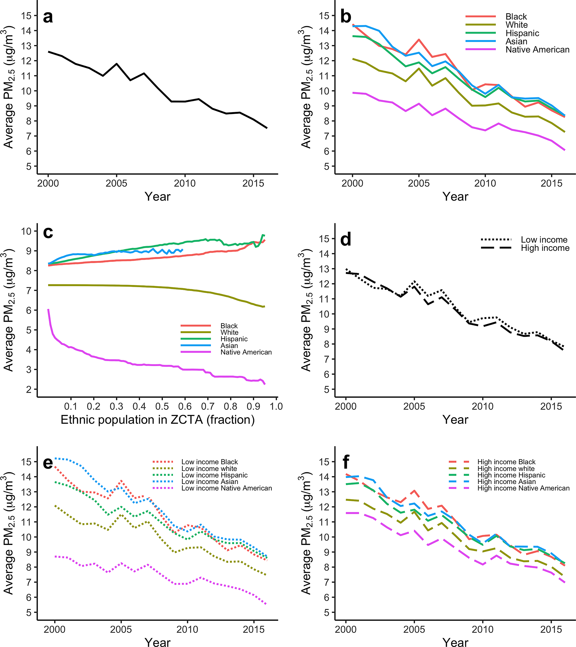
a, Population-weighted average of ${\mathrm{P}\mathrm{M}}_{2.5}$ decreased by 40% from the year 2000 to 2016. b, Population-weighted ${\mathrm{P}\mathrm{M}}_{2.5}$ average concentration across the different racial/ethnic communities for 2000 to 2016. The ${\mathrm{P}\mathrm{M}}_{2.5}$ concentration across the racial/ethnic communities demonstrates that Black and Native American populations live in the most and least polluted areas respectively.c, Population-weighted ${\mathrm{P}\mathrm{M}}_{2.5}$ average concentration across racial/ethnic communities as a function of ZCTA racial/ethnic population (%) for 2016. When the racial/ethnic population % is equal to 0.2, the red curve includes every ZCTA where the Black population is 20% or more, and the blue curve includes every ZCTA where the white population is 20% or more. As ZCTA’s Black and Hispanic or Latino populations increase, the ${\mathrm{P}\mathrm{M}}_{2.5}$ concentration levels increase. The opposite effect is seen for the white and Native American communities. d, Population-weighted ${\mathrm{P}\mathrm{M}}_{2.5}$ average concentration across the income groups reveals that the low-income group is exposed to only slightly higher ${\mathrm{P}\mathrm{M}}_{2.5}$ levels than the high-income groups since 2004. e, The population-weighted ${\mathrm{P}\mathrm{M}}_{2.5}$ average concentration across the different racial/ethnic communities for 2000 to 2016 that are in the low-income group. f, The population-weighted ${\mathrm{P}\mathrm{M}}_{2.5}$ average concentration across the different racial/ethnic communities for 2000 to 2016 that are in the high-income group. Panels e and f show similar differences in ${\mathrm{P}\mathrm{M}}_{2.5}$ average concentrations across the racial/ethnic groups as those of panel b.

Extended Data Figure A.2. Average ${\mathrm{P}\mathrm{M}}_{2.5}$ concentration across the US:

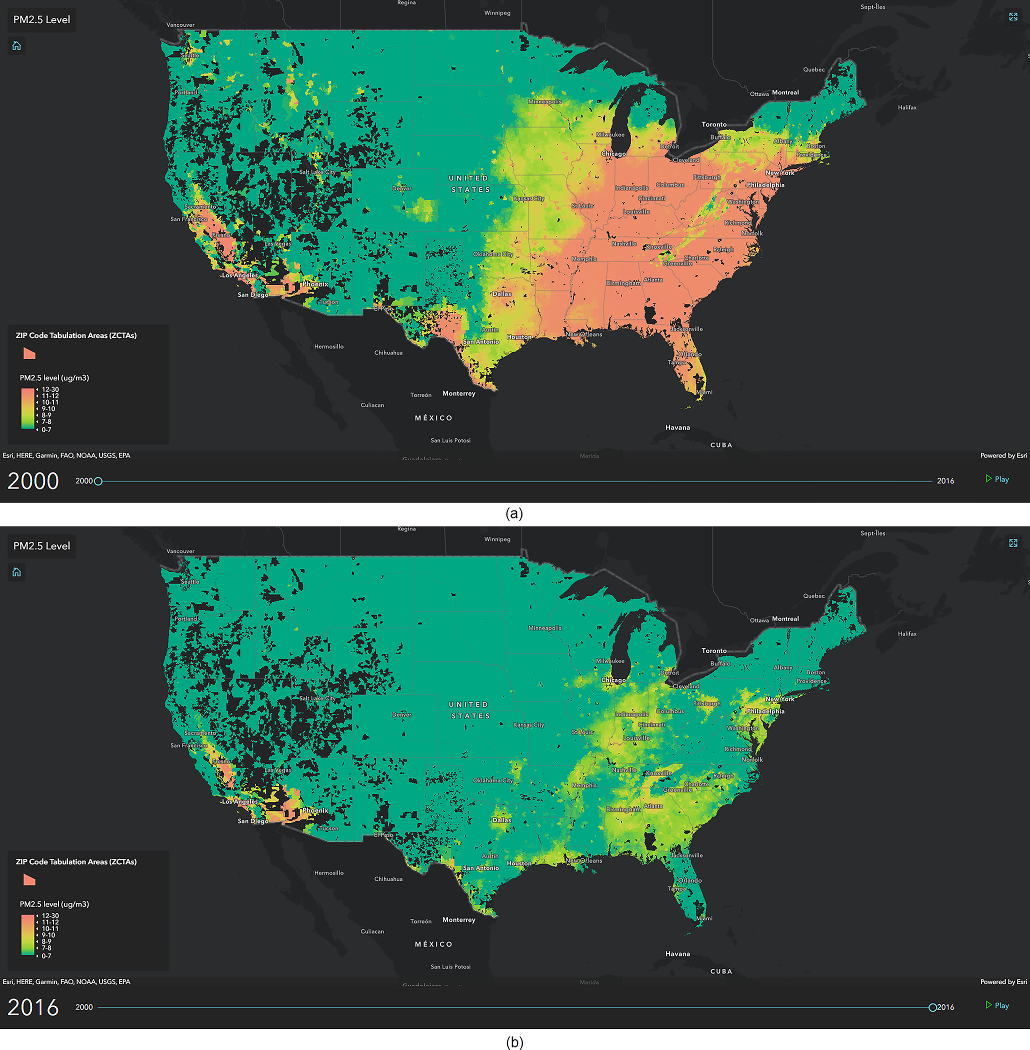
a, Distribution of ${\mathrm{P}\mathrm{M}}_{2.5}$ in 2000. b, Distribution of ${\mathrm{P}\mathrm{M}}_{2.5}$ in 2016. We also include a video that shows the change in the distribution of ${\mathrm{P}\mathrm{M}}_{2.5}$ concentration levels in the US from 2000 to 2016. (video 1).

Extended Data Figure A.3. Average ${\mathrm{P}\mathrm{M}}_{2.5}$ concentration across ZCTAs where different racial/ethnic groups are overrepresented:

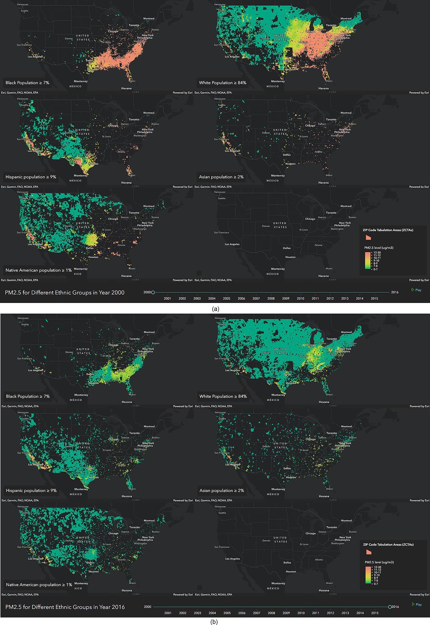
a, Distribution of ${\mathrm{P}\mathrm{M}}_{2.5}$ across five different maps each showing the ZCTAs where one race/ethnicity group is overrepresented for 2000. b, Distribution of ${\mathrm{P}\mathrm{M}}_{2.5}$ across five different maps each showing the ZCTAs where one race/ethnicity group is overrepresented for 2016. We also include an video that shows the change in the distribution of ${\mathrm{P}\mathrm{M}}_{2.5}$ concentration levels across the five maps from 2000 to 2016 (videos 2 and 3).

Extended Data Figure A.4. Distribution of racial/ethnic populations above a ${\mathrm{P}\mathrm{M}}_{2.5}$ threshold of 8 μg/m³ for 2000 and 2016:

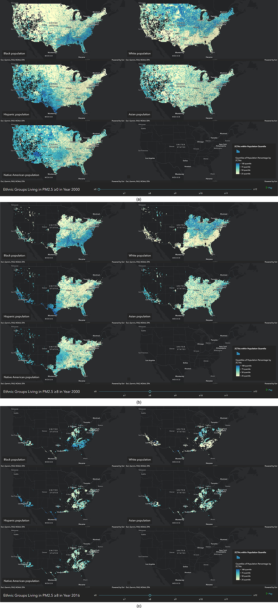
a, US ZCTAs for each race/ethnicity are ranked based on the ratio of the race/ethnicity population to the total ZCTA population. Dark blue indicates fractions close to 1 (ZCTAs where the corresponding race/ethnicity most lives), and light yellow indicates fractions close to 0 (ZCTAs where the corresponding race/ethnicity least lives). b, US ZCTAs above 8 μg/m³ in 2000. c, US ZCTAs above 8 μg/m³ in 2016. We also show the distribution of the different racial/ethnic groups across multiple ranges of ${\mathrm{P}\mathrm{M}}_{2.5}$ concentrations for 2000 and 2016 (videos 5–8).

Extended Data Figure A.5. Supplementary measures of relative disparities in exposure to ${\mathrm{P}\mathrm{M}}_{2.5}$ concentrations from 2000 to 2016 among racial/ethnic groups:

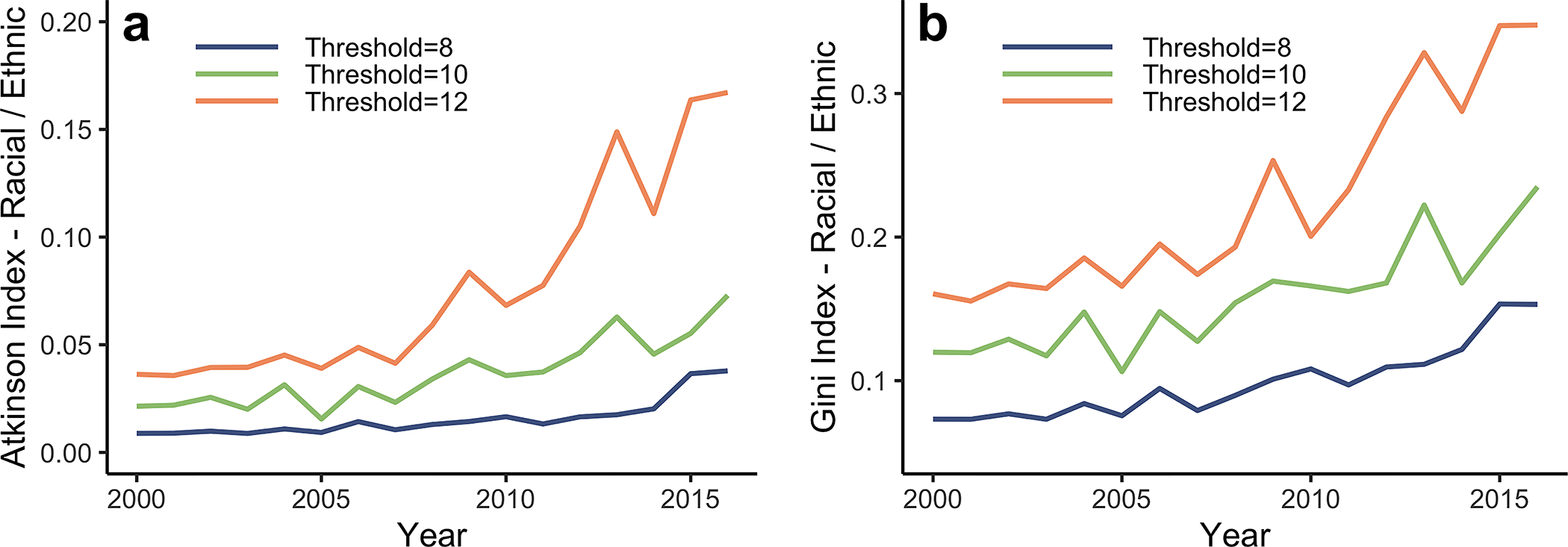
a, The Atkinson index is computed to measure relative disparities among the racial/ethnic groups (Black, white, Asian, Native American and Hispanic or Latino). b, The Gini index is computed to measure relative disparities among the racial/ethnic groups (Black, white, Asian, Native American and Hispanic or Latino). The trends in both the Atkinson and Gini indices are similar to the one measured by CoV in figure 4: disparities in air pollution exposure among racial/ethnic groups relative to pollution levels at or below the EPA standard are increasing. The Atkinson and Gini indices were computed using the inequality package “ineq” in the R software. The input is the proportion of the racial/ethnic (or income) groups living above the set ${\mathrm{P}\mathrm{M}}_{2.5}$ threshold. We set the Atkinson aversion parameter = 0.75 [7], and the sensitivity of the index to different values of is shown in Extended Data Figure A.6.

Extended Data Figure A.6. Sensitivity of the Atkinson index to the inequality aversion parameter:

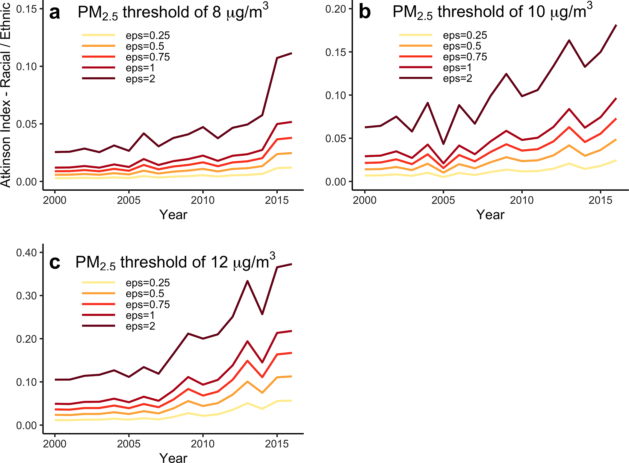
a, Sensitivity of the Atkinson index relative to a ${\mathrm{P}\mathrm{M}}_{2.5}$ threshold of 8 μg/m³. b, Sensitivity of the Atkinson index relative to a ${\mathrm{P}\mathrm{M}}_{2.5}$ threshold of 10 μg/m³. c, Sensitivity of the Atkinson index relative to a ${\mathrm{P}\mathrm{M}}_{2.5}$ threshold of 12 μg/m³. A consistent trend is shown across the parameter values.

Extended Data Figure A.7. Replication of main findings across urban and rural areas:

ZCTA’s population density is used as a metric to control for urbanicity in our study. We classify urban and rural areas based on the percentage of urban population in each ZCTA. Such percentages are available by the census bureau for the year 2010 and are used for the rural/urban classification. ZCTAs with more than 50% urban population are classified in the urban group while those with less than 50% are classified in the rural group. For nationwide, urban and rural US, we reproduce the main results of the manuscript, namely, the average ${\mathrm{P}\mathrm{M}}_{2.5}$ concentrations for the total population (a-c), for racial/ethnic groups (d-f), for income groups (g-i), and disparities across racial/ethnic groups (j-l). Similarities in the results across the national, urban and rural US are apparent and findings are consistent regardless of the urbanicity of ZCTAs. Note that in the case of rural US (l), we only compute disparities for the years where the proportion of the population exposed to ${\mathrm{P}\mathrm{M}}_{2.5}$ concentrations above the thresholds of interest is non-zero. For example, the proportion of population in rural US exposed to ${\mathrm{P}\mathrm{M}}_{2.5}$ concentrations above $T=12\mu \mathrm{g}/m^3$ reaches near zero levels in 2009, and hence disparities after such year are not computed.

Extended Data Figure A.8. Sensitivity of main findings to estimates of ${\mathrm{P}\mathrm{M}}_{2.5}$:

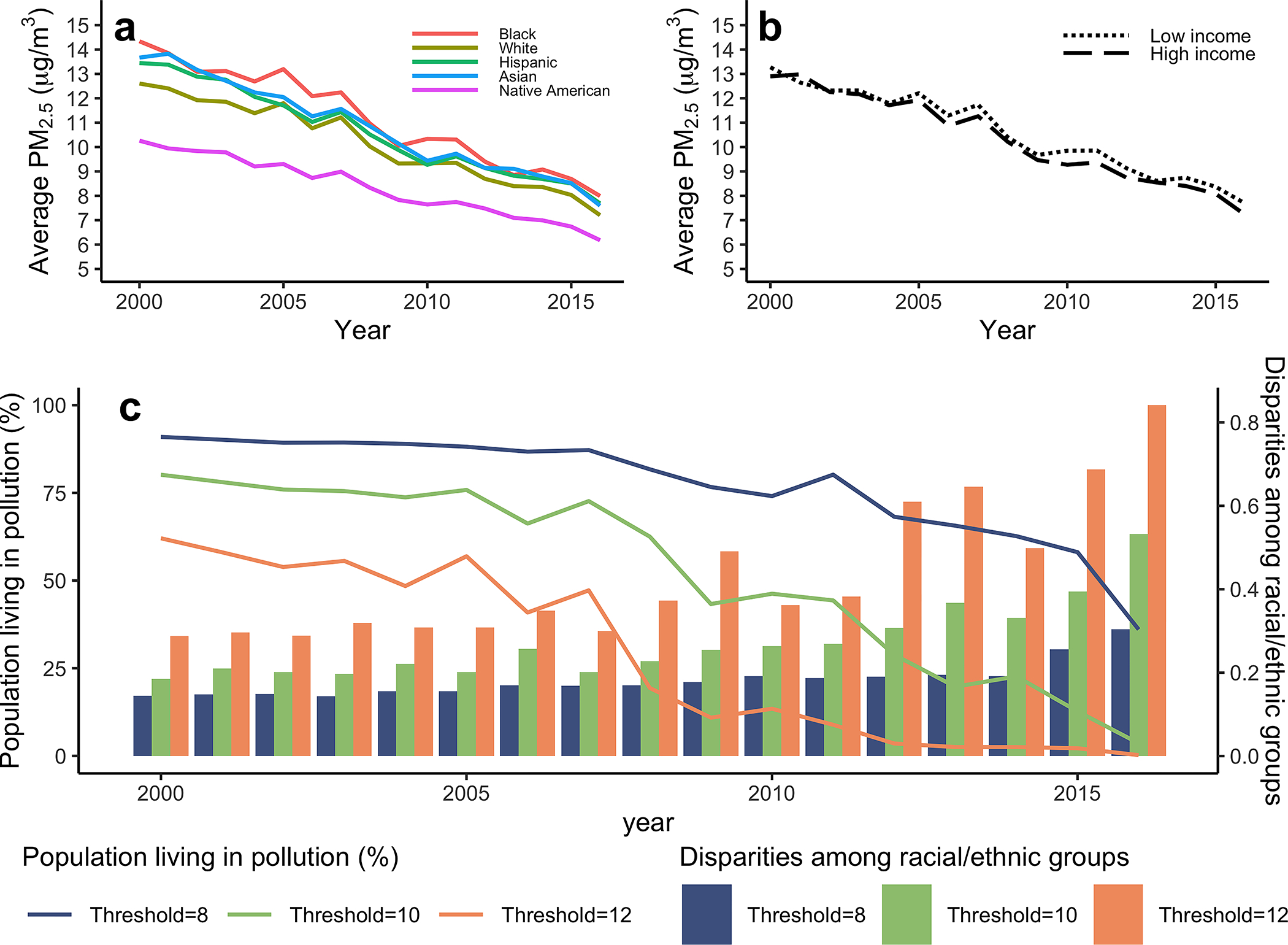
We replicated our analysis with an independent pollution dataset [43, 44] and we show here the sensitivity of our findings to the new ${\mathrm{P}\mathrm{M}}_{2.5}$ estimates. a, Replication of Extended Data figure A.1b with the alternative pollution dataset. b, Replication of Extended Data figure A.1d with alternative pollution dataset. c, Replication of figure 4 with alternative pollution dataset. As can be seen, the main findings of the manuscript are robust and consistent across the two pollution datasets. Minor differences due to the different pollution estimates can be spotted as expected.

Data Availability

Data is available in the following github repositories: https://github.com/NSAPH/National-Causal-Analysis/tree/master/Confounders/census https://github.com/xiaodan-zhou/pm25 and disparity

References

- [1].Cohen AJ, Brauer M, Burnett R, Anderson HR, Frostad J, Estep K, Balakrishnan K, Brunekreef B, Dandona L, Dandona R, et al. , Estimates and 25-year trends of the global burden of disease attributable to ambient air pollution: an analysis of data from the global burden of diseases study 2015, The Lancet 389 (10082) (2017) 1907–1918. [DOI] [PMC free article] [PubMed] [Google Scholar]
- [2].Di Q, Wang Y, Zanobetti A, Wang Y, Koutrakis P, Choirat C, Dominici F, Schwartz JD, Air pollution and mortality in the medicare population, New England Journal of Medicine 376 (26) (2017) 2513–2522. [DOI] [PMC free article] [PubMed] [Google Scholar]
- [3].Bell ML, Zanobetti A, Dominici F, Evidence on vulnerability and susceptibility to health risks associated with short-term exposure to particulate matter: a systematic review and meta-analysis, American journal of epidemiology 178 (6) (2013) 865–876. [DOI] [PMC free article] [PubMed] [Google Scholar]
- [4].Wang Y, Shi L, Lee M, Liu P, Di Q, Zanobetti A, Schwartz JD, Long-term exposure to pm2. 5 and mortality among older adults in the southeastern us, Epidemiology (Cambridge, Mass.) 28 (2) (2017) 207. [DOI] [PMC free article] [PubMed] [Google Scholar]
- [5].Kioumourtzoglou M-A, Schwartz J, James P, Dominici F, Zanobetti A, Pm2. 5 and mortality in 207 us cities: modification by temperature and city characteristics, Epidemiology (Cambridge, Mass.) 27 (2) (2016) 221. [DOI] [PMC free article] [PubMed] [Google Scholar]
- [6].Bell ML, Ebisu K, Environmental inequality in exposures to airborne particulate matter components in the united states, Environmental health perspectives 120 (12) (2012) 1699–1704. [DOI] [PMC free article] [PubMed] [Google Scholar]
- [7].Rosofsky A, Levy JI, Zanobetti A, Janulewicz P, Fabian MP, Temporal trends in air pollution exposure inequality in massachusetts, Environmental research 161 (2018) 76–86. [DOI] [PMC free article] [PubMed] [Google Scholar]
- [8].Mikati I, Benson AF, Luben TJ, Sacks JD, Richmond-Bryant J, Disparities in distribution of particulate matter emission sources by race and poverty status, American journal of public health 108 (4) (2018) 480–485. [DOI] [PMC free article] [PubMed] [Google Scholar]
- [9].Miranda ML, Edwards SE, Keating MH, Paul CJ, Making the environmental justice grade: the relative burden of air pollution exposure in the united states, International journal of environmental research and public health 8 (6) (2011) 1755–1771. [DOI] [PMC free article] [PubMed] [Google Scholar]
- [10].Mohai P, Pellow D, Roberts JT, Environmental justice, Annual review of environment and resources 34 (2009) 405–430. [Google Scholar]
- [11].Agyeman J, Schlosberg D, Craven L, Matthews C, Trends and directions in environmental justice: from inequity to everyday life, community, and just sustainabilities, Annual Review of Environment and Resources 41 (2016). [Google Scholar]
- [12].Banzhaf S, Ma L, Timmins C, Environmental justice: The economics of race, place, and pollution, Journal of Economic Perspectives 33 (1) (2019) 185–208. [PubMed] [Google Scholar]
- [13].Kelly JT, Jang C, Timin B, Di Q, Schwartz J, Liu Y, van Donkelaar A, Martin RV, Berrocal V, Bell ML, Examining pm2. 5 concentrations and exposure using multiple models, Environmental Research (2020) 110432. [DOI] [PMC free article] [PubMed] [Google Scholar]
- [14].Fann N, Coffman E, Timin B, Kelly JT, The estimated change in the level and distribution of pm2. 5-attributable health impacts in the united states: 2005–2014, Environmental research 167 (2018) 506–514. [DOI] [PMC free article] [PubMed] [Google Scholar]
- [15].Tessum CW, Paolella DA, Chambliss SE, Apte JS, Hill JD, Marshall JD, Pm2. 5 polluters disproportionately and systemically affect people of color in the united states, Science Advances 7 (18) (2021). [DOI] [PMC free article] [PubMed] [Google Scholar]
- [16].Harper S, Ruder E, Roman HA, Geggel A, Nweke O, Payne-Sturges D, Levy JI, Using inequality measures to incorporate environmental justice into regulatory analyses, International journal of environmental research and public health 10 (9) (2013) 4039–4059. [DOI] [PMC free article] [PubMed] [Google Scholar]
- [17].Colmer J, Hardman I, Shimshack J, Voorheis J, Disparities in pm2. 5 air pollution in the united states, Science 369 (6503) (2020) 575–578. [DOI] [PubMed] [Google Scholar]
- [18].Meng J, Li C, Martin RV, van Donkelaar A, Hystad P, Brauer M, Estimated long-term (1981–2016) concentrations of ambient fine particulate matter across north america from chemical transport modeling, satellite remote sensing, and ground-based measurements, Environmental science & technology 53 (9) (2019) 5071–5079. [DOI] [PubMed] [Google Scholar]
- [19].US Environmental Protection Agency. Process of reviewing the National Ambient Air Quality Standards., Last Accessed: 2019-12-23. URL https://www.epa.gov/criteria-air-pollutants/process-reviewing-national-ambient-air-quality-standards
- [20].World Health Organization, Air quality guidelines: global update 2005: particulate matter, ozone, nitrogen dioxide, and sulfur dioxide, World Health Organization, 2005. [PubMed] [Google Scholar]
- [21].Dominici F, Peng RD, Bell ML, Pham L, McDermott A, Zeger SL, Samet JM, Fine particulate air pollution and hospital admission for cardiovascular and respiratory diseases, Jama 295 (10) (2006) 1127–1134. [DOI] [PMC free article] [PubMed] [Google Scholar]
- [22].Bell ML, Ebisu K, Peng RD, Walker J, Samet JM, Zeger SL, Dominici F, Seasonal and regional short-term effects of fine particles on hospital admissions in 202 us counties, 1999–2005, American journal of epidemiology 168 (11) (2008) 1301–1310. [DOI] [PMC free article] [PubMed] [Google Scholar]
- [23].Kloog I, Nordio F, Zanobetti A, Coull BA, Koutrakis P, Schwartz JD, Short term effects of particle exposure on hospital admissions in the mid-atlantic states: a population estimate, PloS one 9 (2) (2014). [DOI] [PMC free article] [PubMed] [Google Scholar]
- [24].Bravo MA, Ebisu K, Dominici F, Wang Y, Peng RD, Bell ML, Airborne fine particles and risk of hospital admissions for understudied populations: effects by urbanicity and short-term cumulative exposures in 708 us counties, Environmental health perspectives 125 (4) (2017) 594–601. [DOI] [PMC free article] [PubMed] [Google Scholar]
- [25].Dominici F, McDermott A, Zeger SL, Samet JM, National maps of the effects of particulate matter on mortality: exploring geographical variation., Environmental Health Perspectives 111 (1) (2003) 39–44. [DOI] [PMC free article] [PubMed] [Google Scholar]
- [26].Beelen R, Raaschou-Nielsen O, Stafoggia M, Andersen ZJ, Weinmayr G, Hoffmann B, Wolf K, Samoli E, Fischer P, Nieuwenhuijsen M, et al. , Effects of long-term exposure to air pollution on natural-cause mortality: an analysis of 22 european cohorts within the multicentre escape project, The Lancet 383 (9919) (2014) 785–795. [DOI] [PubMed] [Google Scholar]
- [27].Crouse DL, Peters PA, Hystad P, Brook JR, van Donkelaar A, Martin RV, Villeneuve PJ, Jerrett M, Goldberg MS, Pope III CA, et al. , Ambient pm2. 5, o3, and no2 exposures and associations with mortality over 16 years of follow-up in the canadian census health and environment cohort (canchec), Environmental health perspectives 123 (11) (2015) 1180–1186. [DOI] [PMC free article] [PubMed] [Google Scholar]
- [28].Makar M, Antonelli J, Di Q, Cutler D, Schwartz J, Dominici F, Estimating the causal effect of fine particulate matter levels on death and hospitalization: Are levels below the safety standards harmful?, Epidemiology (Cambridge, Mass.) 28 (5) (2017) 627. [DOI] [PMC free article] [PubMed] [Google Scholar]
- [29].Di Q, Dai L, Wang Y, Zanobetti A, Choirat C, Schwartz JD, Dominici F, Association of short-term exposure to air pollution with mortality in older adults, Jama 318 (24) (2017) 2446–2456. [DOI] [PMC free article] [PubMed] [Google Scholar]
- [30].Wu X, Braun D, Schwartz J, Kioumourtzoglou M, Dominici F, Evaluating the impact of long-term exposure to fine particulate matter on mortality among the elderly, Science Advances (2020) eaba5692. [DOI] [PMC free article] [PubMed] [Google Scholar]
- [31].Liu C, Chen R, Sera F, Vicedo-Cabrera AM, Guo Y, Tong S, Coelho MS, Saldiva PH, Lavigne E, Matus P, et al. , Ambient particulate air pollution and daily mortality in 652 cities, New England Journal of Medicine 381 (8) (2019) 705–715. [DOI] [PMC free article] [PubMed] [Google Scholar]
- [32].Samoli E, Analitis A, Touloumi G, Schwartz J, Anderson HR, Sunyer J, Bisanti L, Zmirou D, Vonk JM, Pekkanen J, et al. , Estimating the exposure–response relationships between particulate matter and mortality within the aphea multicity project, Environmental health perspectives 113 (1) (2005) 88–95. [DOI] [PMC free article] [PubMed] [Google Scholar]
- [33].Samet JM, Dominici F, Curriero FC, Coursac I, Zeger SL, Fine particulate air pollution and mortality in 20 us cities, 1987–1994, New England journal of medicine 343 (24) (2000) 1742–1749. [DOI] [PubMed] [Google Scholar]
- [34].Shah AS, Langrish JP, Nair H, McAllister DA, Hunter AL, Donaldson K, Newby DE, Mills NL, Global association of air pollution and heart failure: a systematic review and meta-analysis, The Lancet 382 (9897) (2013) 1039–1048. [DOI] [PMC free article] [PubMed] [Google Scholar]
- [35].American Psychological Association. Racial and Ethnic Identity, Last Accessed: 2021-08-27. URL https://apastyle.apa.org/style-grammar-guidelines/bias-free-language/racial-ethnic-minorities
- [36].EPA proposes to retain naaqs for particulate matter, Last Accessed: 2020-01-16. URL https://www.epa.gov/newsreleases/epa-proposes-retain-naaqs-particulate-matter
- [37].Clark LP, Millet DB, Marshall JD, National patterns in environmental injustice and inequality: outdoor no2 air pollution in the united states, PloS one 9 (4) (2014) e94431. [DOI] [PMC free article] [PubMed] [Google Scholar]
- [38].Levy JI, Chemerynski SM, Tuchmann JL, Incorporating concepts of inequality and inequity into health benefits analysis, International journal for equity in health 5 (1) (2006) 2. [DOI] [PMC free article] [PubMed] [Google Scholar]
- [39].Lambert PJ, Millimet DL, Slottje D, Inequality aversion and the natural rate of subjective inequality, Journal of Public Economics 87 (5–6) (2003) 1061–1090. [Google Scholar]
- [40].Currie J, Voorheis J, Walker R, What caused racial disparities in particulate exposure to fall? new evidence from the clean air act and satellite-based measures of air quality, Tech. rep., National Bureau of Economic Research (2020). [Google Scholar]
- [41].Auffhammer M, Bento AM, Lowe SE, Measuring the effects of the clean air act amendments on ambient pm10 concentrations: The critical importance of a spatially disaggregated analysis, Journal of Environmental Economics and Management 58 (1) (2009) 15–26. [Google Scholar]
- [42].C. A. Grainger, The distributional effects of pollution regulations: Do renters fully pay for cleaner air?, Journal of Public Economics 96 (9–10) (2012) 840–852. [Google Scholar]
- [43].Di Q, Kloog I, Koutrakis P, Lyapustin A, Wang Y, Schwartz J, Assessing pm2. 5 exposures with high spatiotemporal resolution across the continental united states, Environmental science & technology 50 (9) (2016) 4712–4721. [DOI] [PMC free article] [PubMed] [Google Scholar]
- [44].Di Q, Amini H, Shi L, Kloog I, Silvern R, Kelly J, Sabath MB, Choirat C, Koutrakis P, Lyapustin A, et al. , An ensemble-based model of pm2. 5 concentration across the contiguous united states with high spatiotemporal resolution, Environment international 130 (2019) 104909. [DOI] [PMC free article] [PubMed] [Google Scholar]
Associated Data
This section collects any data citations, data availability statements, or supplementary materials included in this article.
Supplementary Materials
Data Availability Statement