Generalized Phase I-II Designs to Increase Long Term Therapeutic Success Rate

Abstract

Designs for early phase dose finding clinical trials typically are either phase I based on toxicity, or phase I-II based on toxicity and efficacy. These designs rely on the implicit assumption that the dose of an experimental agent chosen using these short-term outcomes will maximize the agent’s long-term therapeutic success rate. In many clinical settings, this assumption is not true. A dose selected in an early phase oncology trial may give suboptimal progression free survival or overall survival time, often due to a high rate of relapse following response. To address this problem, a new family of Bayesian generalized phase I-II designs is proposed. First, a conventional phase I-II design based on short-term outcomes is used to identify a set of candidate doses, rather than selecting one dose. Additional patients then are randomized among the candidates, patients are followed for a predefined longer time period, and a final dose is selected to maximize the long term therapeutic success rate, defined in terms of duration of response. Dose-specific sample sizes in the randomization are determined adaptively to obtain a desired level of selection reliability. The design was motivated by a phase I-II trial to find an optimal dose of natural killer cells as targeted immunotherapy for recurrent or treatment-resistant B-cell hematologic malignancies. A simulation study shows that, under a range of scenarios in the context of this trial, the proposed design has much better performance than two conventional phase I-II designs.

1. Introduction

1.1. Conventional Dose Finding Designs

Adoptive T-cell therapy uses immune cells engineered to attack a specific disease target. Cell therapy has been used to treat leukemia and lymphoma [1, 2], and diseases such as type 1 diabetes, Parkinson’s disease, and Alzheimer’s disease. The dose-finding design proposed in this paper was motivated by an early phase trial of CD70 CAR natural killer (NK) cells as targeted immunotherapy for recurrent or treatment-resistant B-cell hematologic malignancies following frontline treatment with chemotherapy or an allogeneic stem cell transplant. The therapeutic aims are to achieve a disease remission, and reduce the rate of subsequent disease recurrence. Treatment begins with three days of chemotherapy to debulk the patient’s disease, followed by one infusion of NK cells at a selected dose. The primary scientific goal is to optimize dose among the four values $5.0\times \hspace{0.17em}\hspace{0.17em}\left({10}^6,{10}^7,{10}^8,{10}^9\right)$ cells.

Initially, a conventional phase I-II design for this trial was based on indicators Y_R of response at one month, and Y_T of grade 3 or 4 toxicity within one month of cell infusion. The plan was to treat up to 48 patients in 16 cohorts of size three, starting at the lowest dose, with the following screening rules. For dose d, and binary toxicity and response indicators Y_T and Y_R, denote ${\pi }_R\left(d,\mathit{\theta }\right)=\text{Pr}\left(Y_R=1|d,\mathit{\theta }\right)$, ${\pi }_T\left(d,\mathit{\theta }\right)=\text{Pr}\left(Y_T=1|d,\mathit{\theta }\right)$, and ${𝓓}_n$ the data from n patients. Given lower limit .50 on ${\pi }_R\left(d,\mathit{\theta }\right)$ and upper limit .30 on ${\pi }_T\left(d,\mathit{\theta }\right)$, a dose d was considered acceptable if

$$\text{Pr}\left\{{\pi }_R\left(d,\mathit{\theta }\right)>.50|{𝓓}_n\right\}>.10andPr\left\{{\pi }_T\left(d,\mathit{\theta }\right)<.30|{𝓓}_n\right\}>\mathrm{.10.}$$ (1)

Bayesian dose acceptability criteria of this form have been used in many phase I-II designs [3, 4, 5]. Subsequently, a more general design was motivated by concerns about response durability, since a patient’s disease may recur soon after a response is achieved. The investigators planned to follow each patient for up to six months to assess whether they were alive with disease in remission at that time. This led to consideration of how data from this later evaluation might be used to help choose an optimal dose. The result is the generalized phase I-II design presented here, which we call Gen I-II.

Most early phase trials determine a dose using either a phase I design based on Y_T, or a phase I-II design based on bivariate binary or ordinal (Y_R, Y_T) and Y_R. In oncology, examples of binary response include 50% reduction of a solid tumor or complete remission of acute leukemia. Most of these designs use sequentially outcome-adaptive rules to choose doses for successive patient cohorts. Fair randomization among doses seldom is used, due to concerns that higher doses may be unacceptably toxic. Many phase I designs [6, 7, 8, 9] and phase I-II designs [3, 10, 11, 12, 13, 14, 15, 16] have been proposed. Most of these designs use binary outcomes, although phase I-II designs have been proposed for ordinal outcomes [17], event times [18, 19], or more than two outcomes [5, 20].

A practical requirement in dose finding trials is that the outcomes, Y_T or Y = (Y_R, Y_T), must be evaluated over a time period, [0, t₁], short enough to avoid delaying accrual to evaluate previous patients’ outcomes to make adaptive decisions. For designs based on event times, such as the phase I time-to-event continual reassessment method (TITE-CRM) [37] or late-onset efficacy-toxicity phase I-II design [22], follow up intervals must be short enough so that outcome-adaptive decisions can be made without unduly suspending accrual.

1.2. A Dose Finding Trial That Failed

A conventional dose finding design may fail if there is a disconnect between short-term response and long term outcomes, such as disease progression or overall survival (OS) time. This problem arose in a trial of allogeneic stem cell transplantation for acute leukemia [23]. to optimize the dose of vorinostat added to a standard preparative regimen. Six doses were studied using the TiTE-CRM with target toxicity probability 0.30, followed by an expansion cohort at the selected dose. Toxicity was defined as graft failure or grade 4 or 5 non-hematologic, non-infectious toxicity, mucositis, or diarrhea within one month, For response defined as the patient being alive and engrafted at one month, this definition of DLT includes non-response, due to death or graft failure within one month, so this was a phase I-II trial. Since very few DLTs were observed, the TiTE-CRM design rapidly escalated and selected the highest dose as the MTD, where 51 patients were treated, most as an expansion cohort. The final sample sizes were (3, 3, 3, 4, 4, 51) at the six doses. Analysis of the final survival data gave the Kaplan-Meier estimates for doses {1, 2, 3, 4, 5} combined versus dose 6 in Figure 1, showing that patients treated with the selected dose 6 had worse survival than patients given one of the five lower doses. While these results are far from confirmatory, they are very troubling. To design a future trial, the highest dose is undesirable but a lower dose giving superior survival time cannot be determined reliably from the data. Since this trial is unlikely to be repeated, there is no clear path forward. This trial illustrates a disconnect between short term outcomes and dose effects on progression or survival time.

Figure 1:

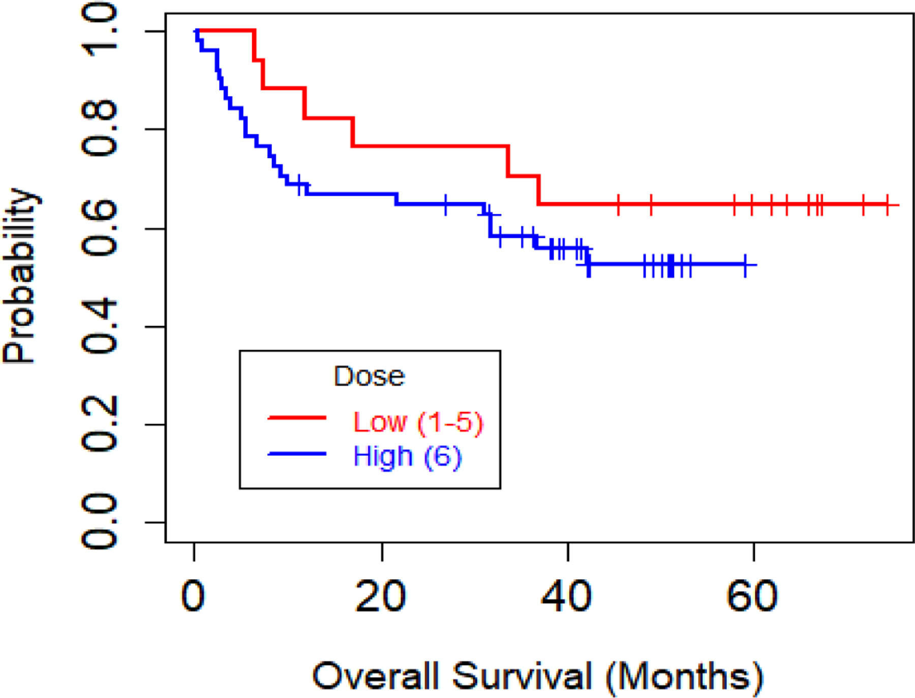
Kaplan-Meier plot of overall survival (OS) for the acute leukemia phase I trial by dose group, defined as Low (doses 1–5 combined) or High (dose 6).

1.3. A Flawed Assumption

Phase I and I-II designs assume that, if d is optimal based on a criterion defined using early outcomes, then d also maximizes the therapeutic success rate over a long-term follow up period [0, t₂], for $t_2>t_1$. To account for this in the Gen I-II design, given fixed t₁ and t₂, we define duration of response (DOR), Z, among responders as the time from t₁ to relapse or death. The long-term treatment success criterion is the probability

$$\xi \left(d,\mathit{\theta }\right){=}_{def}\text{Pr}\left(Z>t_2-t_1|d,\mathit{\theta }\right),$$ (2)

where θ denotes the model parameter vector. Expression (2) is the probability that a patient who is alive with disease in remission at t₁ is alive without progressive disease (PD) at t₂.

The Gen I-II design addresses the common problem in oncology that an early response may not be durable, in that a patient who responds by t₁ may relapse before t₂. Consequently, a dose optimizing $\varphi \left(d,\mathit{\theta }\right)$ may not optimize $\xi \left(d,\mathit{\theta }\right)$. Response durability has been discussed for radiation oncology [24], donor lymphocyte infusion following relapse after allogeneic bone marrow transplantation [25], and many other areas of oncology. The Gen I-II design is practical in settings where investigators planning a phase I-II trial intend to follow each patient for a longer time t₂, to obtain data to estimate response durability. Thus, no additional followup is required beyond what already is planned. A dose chosen in an early phase trial may be suboptimal because the distribution of (Y_R, Y_T) provides little information about the time to progression or death as a function of dose. This problem is more severe with phase I designs. Since phase I designs have severe flaws compared to phase I-II designs[12, 26, 27], we will not consider phase I designs further.

A Gen I-II design uses the distributions of ordinal Y_R and Y_T evaluated over [0, t₁] and Z evaluated over [t₁, t₂] among responders to optimize d. Let $\varphi \left(d,\mathit{\theta }\right)$ be an objective function, defined in terms of the early outcome distribution $p\left(\mathit{Y}|d,\mathit{\theta }\right)$, used to optimize d in phase I-II. Examples of $\varphi \left(d,\mathit{\theta }\right)$ will be given below. Denote the experimental agent by X, and let X(d) denote X administered at d, to account for the possibility that effects of X(d) and X(d′) on Y or Z may be different for $d\ne d\prime$. While we use the long-term success criterion $\xi \left(d,\mathit{\theta }\right)=\text{Pr}\left(Z>t_2-t_1|d,\mathit{\theta }\right)$, the mean $E\left(Z|d,\mathit{\theta }\right)$ may be used. The implicit assumption underlying phase I-II trials is that, if a selected dose $d^{sel,\varphi }$ maximizes an estimate of $\varphi \left(d,\mathit{\theta }\right)$ at the end of phase I-II, then $d^{sel,\varphi }$ also maximizes $\xi \left(d,\mathit{\theta }\right)$. The validity of this assumption depends on how $p\left(\mathbf{Y}|d,\mathit{\theta }\right)$ and $p\left(Z|d,\mathit{\theta }\right)$ vary with d, and associations between Z and Y. Conventionally, using $\varphi \left(d,\mathit{\theta }\right)$ rather than $\xi \left(d,\mathit{\theta }\right)$ to optimize d is motivated primarily by the desire for logistical convenience when conducting a dose-finding trial.

It is easy to show by example that, for assumed true values ${\varphi }^{true}\left(d,\mathit{\theta }\right)$ and ${\xi }^{true}\left(d,\mathit{\theta }\right)$, the optimal doses $d^{opt,\varphi }$ and $d^{opt,\xi }$ under the two criteria may differ. Several scenarios reflecting this possibility are included in the simulations given below in Section 5. Even if Z depends on Y, an optimal phase I-II dose $d^{sel,\varphi }$ based on $\varphi \left(d,\mathit{\theta }\right)$ may be suboptimal in terms of $\xi \left(d,\mathit{\theta }\right)$. A causal explanation with targeted agents or cellular therapies is that there may be direct biological effects of X(d) on Z not mediated by Y_R. This is a version of the general problem when dealing with relationships between short-term and long-term outcomes in treatment evaluation, which has been discussed extensively, often with regard to using an early outcome as a surrogate for a long-term outcome. Common examples are response and PFS time, and the times to PD and death [28, 29, 30, 31].

Section 2 presents the general Gen I-II design paradigm. Dose-outcome models are given in section 3. Section 4 describes a utility based version of the Gen I-II design. A simulation study of the Gen I-II design and two conventional phase I-II designs is presented in section 5. We close with a discussion in section 6.

2. A Generalized Phase I-II Design Paradigm

2.1. Overview of the Design

A Gen I-II design begins with a conventional phase I-II design based on ordinal, possibly binary Y_R and Y_T, to screen out unsafe or ineffective doses, and identify a set $𝓒$ of acceptable candidate doses for later evaluation, rather than selecting one final dose. Additional patients are randomized among the doses in $𝓒$ and followed to evaluate the times to progression or death, with a final dose selected to maximize $\xi \left(d,\mathit{\theta }\right)$ for $d\in 𝓒$. The number of additional patients enrolled after the initial phase I-II portion of the trial is determined adaptively, based on $𝓒$ and the numbers of patients treated at its doses, to obtain a high probability of correctly selecting a dose to maximize $\xi \left(d,\mathit{\theta }\right)$ for $d\in 𝓒$. The additional patients may be thought of as a generalized expansion cohort, but randomized among the doses in $𝓒$, rather than being treated at one dose that may turn out to be suboptimal. The Gen I-II design is a modular paradigm in that any phase I-II design based on bivariate ordinal Y may be used, provided that it includes a dose optimality criterion $\varphi \left(d,\mathit{\theta }\right)$.

A Gen I-II design has three stages. Stages 1 and 2 together comprise the nominally “phase I-II” portion of the trial. In stage 1, a conventional phase I-II design is based on Y evaluated over [0, t₁]. Any phase I-II design with an objective function $\varphi \left(d,\mathit{\theta }\right)$ characterizing dose desirability may be used. In stage 2, doses are chosen using adaptive randomization (AR) with probabilities defined in terms of $\varphi \left(d,\mathit{\theta }\right)$. At the end of stage 2, a set $𝓒$ of candidate doses with estimated $\varphi \left(d,\mathit{\theta }\right)$ close to the maximum estimate is determined. In stage 3, additional patients are randomized among the doses in $𝓒$, and all patients are followed for a longer period [0, t₂] to obtain data on (d, Z). At the end of stage 3, the candidate dose maximizing the posterior mean of $\xi \left(d,\mathit{\theta }\right)$ is selected.

2.2. Design Construction and Trial Conduct

A Gen I-II design may be constructed in numerous ways, depending on how Y and $\varphi \left(d,\mathit{\theta }\right)$ are defined and the probability models $p\left(\mathit{Y}|d,\mathit{\theta }\right)$ and $p\left(Z|d,\mathit{\theta }\right)$. To make things concrete for the Gen I-II design that we will use to illustrate the methodology, we define the early outcomes, evaluated over the interval [0, t₁], to be a binary indicator variable Y_T of toxicity and a three-level ordinal response variable $Y_R^{\prime }$ taking on the possible values $Y_R^{\prime }=2$ for response (RES), $Y_R^{\prime }=1$ for stable disease (SD), and $Y_R^{\prime }=0$ for progressive disease or death (PD). Denoting the indicator of the event A by I[A], we define the binary response indicator $Y_R=I\left[Y_R^{\prime }=2\right]$. We include the third event $\text{SD}={\left(RES\cup PD\right)}^c=\left[Y_R^{\prime }=1\right]$ to accommodate settings where RES and PD are not complementary, that is, a patient may not have a response but this was not due to early PD. Other early outcomes may be used, including ordinal toxicity with three or more levels of severity, or $Y_R^{\prime }$ with more than three levels, with appropriate modifications of the Gen I-II design parameters. When either Y_R or Y_T has three or more ordinal levels, a binary version of each must be defined in order to specify the dose admissibility criteria (1).

Denote the Gen I-II stage s sample size by n_s for s = 1, 2, 3, and overall sample size $N=n_1+n_2+n_3$. Values of n₁ and n₂ are specified at the start of the trial, but n₃ is determined adaptively at the end of stage 2 to obtain a desired level of final dose selection reliability, as described below. Examples of $\varphi \left(d,\mathit{\theta }\right)$ based on bivariate binary Y = (Y_R, Y_T) include the response probability ${\pi }_R\left(d,\mathit{\theta }\right)$ [33], the odds ratio defined in terms of ${\pi }_R\left(d,\mathit{\theta }\right)$ and ${\pi }_T\left(d,\mathit{\theta }\right)$, and the trade-off function $f\left\{{\pi }_R\left(d,\mathit{\theta }\right),\hspace{0.17em}\hspace{0.17em}{\pi }_T\left(d,\mathit{\theta }\right)\right\}$ used by the EffTox design [3, 34]. If numerical outcome utilities, U(Y), are elicited, then the optimality criterion may be the mean utility $\varphi \left(d,\mathit{\theta }\right)=E\left\{U\left(\mathit{Y}\right)|d,\mathit{\theta }\right\}$ [5, 14, 15, 16, 17, 35, 36]. In our construction of a Gen I-II design, below, we take a utility based approach with $\mathbf{Y}=\left(Y_R^{\prime },Y_T\right)$.

For the i^th patient enrolled in a Gen I-II trial, denote the assigned dose by d_[i] and let V_i be the independent right censoring time of Z_i starting from the time t₁ when $Y_{i,R}^{\prime }$ is evaluated, conditional on $Y_{i,R}^{\prime }>0$. The observed time to failure or censoring following t₁ is thus $Z_i^o=min\left\{Z_i,V_i\right\}$. Let ${\delta }_i=1$ if $Z_i^o=Z_i$ and ${\delta }_i=0$ if $Z_i^o=V_i<Z_i$, so the data from the first n patients enrolled in the trial is

$${𝓓}_n=\left\{\left(Y_{i,R}^{\prime },Y_{i,T},Z_i^o,{\delta }_i,d_{\left[i\right]}\right)\hspace{0.17em}\hspace{0.17em}\hspace{0.17em}:\hspace{0.17em}\hspace{0.17em}\hspace{0.17em}i=1,\hspace{0.17em}\hspace{0.17em}\cdots \hspace{0.17em}\hspace{0.17em},n\right\}.$$ (3)

Stages 1 and 2 of the Gen I-II design include dose acceptability criteria of the form given in equation (1), with fixed lower limit ${\underset{¯}{\pi }}_R$ for response probability and upper limit ${\overline{\pi }}_T$ for toxicity probability. Denote the set of acceptable doses satisfying (1) by ${𝓐}_n$. During stages 1 and 2, no patient is treated with an unacceptable dose, and if it is determined that no dose is acceptable, the trial is stopped, stage 3 is not conducted, and no dose is selected.

Denote $n_{1,2}=n_1+n_2$. For each dose d_j, $j\hspace{0.17em}\hspace{0.17em}=\hspace{0.17em}\hspace{0.17em}1,\hspace{0.17em}\hspace{0.17em}\cdots \hspace{0.17em}\hspace{0.17em},J$ and $n\hspace{0.17em}\hspace{0.17em}=\hspace{0.17em}\hspace{0.17em}1,\hspace{0.17em}\hspace{0.17em}\cdots \hspace{0.17em}\hspace{0.17em},n_{1,2}$, denote ${\widehat{\varphi }}_{j,n} =E\left\{\varphi \left(d_j,\mathit{\theta }\right)|{𝓓}_n\right\}$. In stage 1, doses are chosen to maximize ${\widehat{\varphi }}_{j,n}$ for n₁ patients. In stage 2, doses are chosen for n₂ patients using AR. Given a fixed shrinkage parameter $0<\hspace{0.17em}\hspace{0.17em}\zeta \le \hspace{0.17em}\hspace{0.17em}1$, AR probabilities may be defined to be proportional to ${\left({\widehat{\varphi }}_{j,n}\right)}^{\zeta }$. A formula for the AR probabilities is given in the Supplement. Compared to maximizing ${\widehat{\varphi }}_{j,n}$, AR distributes patients more evenly among acceptable doses during stage 2, which gives a more even distribution of patients among the candidate doses. While using AR is not a requirement of the Gen I-II design, our simulations will show that AR improves final correct selection probabilities and reduces additional stage 3 per-dose sample sizes.

At the end of stage 2, given fixed $0<\rho <1$, the candidate dose set is defined to be all $d_j\in {𝓐}_{n_{1,2}}$ with posterior mean desirability close to the maximum value,

$$𝓒=\left\{d_j\in {𝓐}_{n_{1,2}}\hspace{0.17em}\hspace{0.17em}:\hspace{0.17em}\hspace{0.17em}{\widehat{\varphi }}_{j,n_{1,2}}\ge \rho \underset{d_l\in {𝓐}_{n_{1,2}}}{\max }{\widehat{\varphi }}_{l,n_{1,2}}\right\}.$$ (4)

The parameter ρ determines how close the estimated optimality criterion of a dose must be to the maximum for it to be in $𝓒$. Preliminary simulations examining several numerical values, such as ρ = .60, .70, and .80, should be used to identify a value giving a design with good OCs. The value $\rho =.70$ was chosen for the CAR NK cell Gen I-II trial design.

The stage 3 sample size n₃ is determined adaptively using the data ${𝓓}_{n_{1,2}}$ and the per-dose subsample sizes $\left\{n_{1,2}\left(d_j\right)\hspace{0.17em}\hspace{0.17em}:\hspace{0.17em}\hspace{0.17em}{d}_j\in 𝓒\right\}$ at the end of stage 2. The $n_{1,2}\left(d_j\right)$ values are random because doses are chosen adaptively in stages 1 and 2. Denote the stage 3 sample size of dose $d_j\in 𝓒$ by $n_3\left(d_j\right)$, so that $n_3={\sum }_{d_j\in 𝓒}{n}_3\left(d_j\right)$ and the per-dose sample sizes from all three stages are $N\left(d_j\right)=n_1\left(d_j\right)+n_2\left(d_j\right)+n_3\left(d_j\right)$. To determine $n_3\left(d_j\right)$ adaptively, we choose a fixed overall per dose sample size $N\left(d\right)=N\left(d_j\right)$ for all j that ensures a desired level of reliability for selecting an optimal dose from $𝓒$ at the end of the trial. Since $𝓒$ is a random set, the value of N (d) may be chosen from several feasible values, such as N(d) = 10, 15, or 20. This is done based on simulations of the trial, for given n₁, n₂, ρ, and assumed true values of the long term success probabilities, ${\mathit{\xi }}^{true}=\left({\xi }^{true}\left(d_1\right),···,{\xi }^{true}\left(d_J\right)\right)$, and short term success probabilities, ${\varphi }^{true}=\left({\varphi }^{true}\left(d_1\right),\cdots ,{\varphi }^{true}\left(d_J\right)\right)$. Each $n_3\left(d_j\right)=N\left(d_j\right)-n_{1,2}\left(d_j\right)$ depends on $𝓒$ and the values of n_1,2(d_j) for the candidate doses $d_j\in 𝓒$. For example, if J = 4, $𝓒=\left\{d_3,d_4\right\}$, n_1,2(d₃) = 12, and n_1,2(d₄) = 6, then N(d) = 20 requires n₃(d₃) = 8 and n₃(d₄) = 14. Thus, in stage 3 a total of 22 additional patients would be randomized between d₃ and d₄, restricted to obtain overall per-dose sample sizes of 20.

To illustrate the per-dose sample size determination process between stages 2 and 3, we use scenario 3 of our simulation study, which is given in detail in Table S1 of the supplementary materials. We consider three different combinations of the total sample size n₂ used in stage 2 and total sample N(d) at d, specifically (n₂, N(d)) = (39,9), (33,15), and (27,21). Simulations of the Gen I-II design under scenario 3 using each of these sample size configurations show that (n₂, N(d)) = (39,9) gives very slightly worse results than (33,15) in terms of both the optimal dose selection percentages (70.0% vs 70.5%) and average total sample sizes (53.2 vs 52.7). The combination (27,21) gives the highest optimal dose selection percentage of 74.9%, but larger average total sample size 65.2. The sample size setting (n₂, N(d)) = (33, 15) was chosen by considering the tradeoff between correct true optimal dose selection percentage and sample size. In this setting, if the investigators were willing to treat an expected total of about 65 – 48 = 17 more patients in stage 3, rather than 53 – 48 = 5 more, as the price to obtain an improvement from 70.5% to 74.9% in optimal dose selection percentage, then the third pair (n₂, N(d)) = (27, 21) could be used.

For the final dose selection, we require each $d\in 𝓒$ to satisfy the additional long-term success probability acceptability requirement

$$Pr\left\{\xi \left(d,\mathit{\theta }\right)>\underset{\_}{\xi } |{𝓓}_N\right\}>.10,$$ (5)

where $\underset{\_}{\xi }$ is a fixed lower limit for $\xi \left(d_j,\mathit{\theta }\right)$. Denote the final set of acceptable doses in $𝓒$ by ${𝓐}_N^{\xi }$. The futility requirement (5) reduces the chance of selecting a dose from a set of candidates that all are unlikely to have a long term success rate at least $\underset{\_}{\xi }$. In practice, $\underset{\_}{\xi }$ may be the historical mean of ξ with standard therapy. The final selected optimal dose in the acceptable dose set ${𝓐}_N^{\xi }$ is defined to maximize the posterior mean long term success probability,

$$d_N^{sel,\xi }=\underset{d_j\in {𝓐}_N^{\xi }}{\text{argmax}}E\left\{\xi \left(d_j,\mathit{\theta }\right)\left.|{𝓓}_N\right)\right\}.$$ (6)

Figure 2 provides a schematic for Gen I-II design conduct. The design parameters include values required to specify the phase I-II design and objective function $\varphi \left(d,\mathit{\theta }\right)$ used in stages 1 and 2, including t₁, n₁, n₂, cohort size c, acceptability limits ${\underset{¯}{\pi }}_E$ and ${\overline{\pi }}_T$, and the exponent ζ used to define the AR probabilities. For stage 3, one must specify the long-term follow up time t₂, ρ, $\underset{\_}{\xi }$, and the overall per-dose sample size N(d) required for each $d_j\in 𝓒$.

Figure 2:

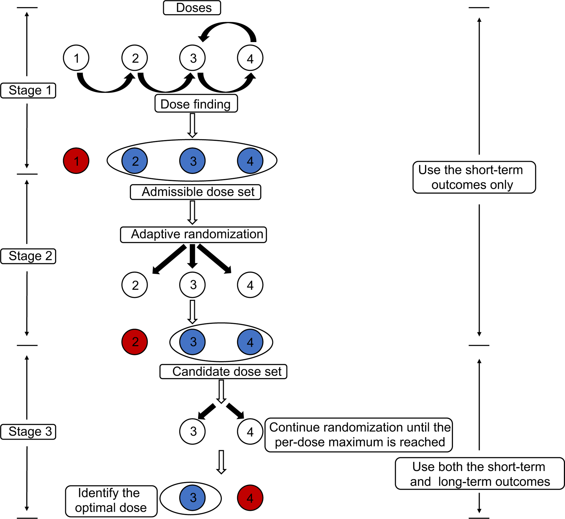
Schematic for the Gen I-II design.

We assume a Bayesian model to exploit the Bayesian paradigm’s ability to fully account for uncertainty and provide shrinkage toward the prior for posterior criteria used to make decisions. For the Bayesian model, one must specify hyperparameters ${\tilde{\mathit{\theta }}}_1$ of the noninformative prior $p\left({\mathit{\theta }}_1|{\tilde{\mathit{\theta }}}_1\right)$ in the model for $p\left(\mathbf{Y}|d,{\mathit{\theta }}_1\right)$, and hyperparameters ${\tilde{\mathit{\theta }}}_2$ of the noninformative prior $p\left({\mathit{\theta }}_1|{\tilde{\mathit{\theta }}}_2\right)$ in the conditional failure time distribution $p\left(Z|d,\mathbf{Y},{\mathit{\theta }}_2\right)$.

3. Dose Outcome Models

We assume the following Bayesian multinomial-Dirichlet model for the early outcome $\mathbf{Y}=\left(Y_R^{\prime },Y_T\right)$. More elaborate models may be used, but we found that this model gives a design with good properties while avoiding possibly restrictive assumptions. For each dose d₁, …, d_J, and outcome indices a = 0, 1, 2 for $Y_R^{\prime }$ and b = 0, 1 for Y_T, denote the joint probability $p_{a,b}\left(d_j\right)=Pr\left(Y_R^{\prime }=a,Y_T=b | d_j\right)$, with $\mathbf{p}\left(d_j\right)=\left(p_{0,1}\left(d_j\right),\hspace{0.17em}\hspace{0.17em}\cdots \hspace{0.17em}\hspace{0.17em},p_{1,2}\left(d_j\right)\hspace{0.17em}\right)$. Thus, the model parameter vector is ${\mathit{\theta }}_1=\left(\mathbf{p}\left(d_1\right),\hspace{0.17em}···\hspace{0.17em}\hspace{0.17em},\mathbf{p}\left(d_J\right)\right)$. For each dose d_j and interim sample size n, we assume that the six-dimensional outcome count vector

$$X_n\left(d_j\right)=\sum _{i=1}^n\left(I\left[\mathbf{Y}=\left(0,0\right)\right],\hspace{0.17em}\cdots \hspace{0.17em},I\left[\mathbf{Y}=\left(2,1\right)\right]\right)\hspace{0.17em}\hspace{0.17em}I\left[d_{\left[i\right]}=d_j\right]$$

is multinomial with parameters n(d_j) and p(d_j), and that p(d_j) follows a Dirichlet prior with parameter 1/6 in each cell. While this model does not borrow strength between doses, it is robust since it makes no assumptions about dose-response curves, and facilitates posterior computation because $\mathbf{p}\left(d_j\right)|{\mathbf{X}}_n\left(d_j\right)$ is Dirichlet with parameters $\left(1/6,\hspace{0.17em}\hspace{0.17em}\cdots \hspace{0.17em},\hspace{0.17em}1/6\right)+{\mathbf{X}}_n\left(d_j\right)$ for each d_j. The early outcome objective function is the mean utility

$$\varphi \left(d_j,{\mathit{\theta }}_1\right)=\overline{U}\left(d_j,{\mathit{\theta }}_1\right)=\sum _{a=0}^2\sum _{b=0}^{1}U\left(a,b\right)p_{a,b}\left(d_j\right)\hspace{0.17em}\hspace{0.17em}\hspace{0.17em}\text{for}\hspace{0.17em}\hspace{0.17em}\hspace{0.17em}j=1,\hspace{0.17em}\cdots \hspace{0.17em}\hspace{0.17em},J.$$ (7)

This Multinomial-Dirichlet model and definition of $\varphi \left(d_j,{\mathit{\theta }}_1\right)$ may be extended easily to accommodate any discrete bivariate ordinal $\left(Y_T,Y_R^{\prime }\right)$.

For the distribution of Z, due to limited sample size a flexible but parsimonious model is needed. We thus assume that Z follows a Weibull distribution with pdf

$$f_Z\left(z|Y_T,d_{j,}{\mathit{\theta }}_2\right)=\frac{\alpha }{\lambda }{\left(\frac{z}{\lambda }\right)}^{\alpha -1}\hspace{0.17em}\hspace{0.17em}\text{exp}\left\{-{\left(z/\lambda \right)}^{\alpha }\right\},\hspace{0.17em}\hspace{0.17em}\hspace{0.17em}\hspace{0.17em}\hspace{0.17em}\hspace{0.17em}\hspace{0.17em}z>0,$$

where α > 0 is the shape parameter and the rate parameter λ is given by

$$\lambda \left(Y_T,d_j,{\mathit{\theta }}_2\right)=exp\left({\beta }_0+{\beta }_T\hspace{0.17em}{Y}_T+{\gamma }_j\right)$$ (8)

with γ₁ = 0. We denote ${\mathit{\theta }}_2=\left(\alpha ,{\beta }_0,{\beta }_T,{\gamma }_2,\hspace{0.17em}\cdots \hspace{0.17em},{\gamma }_J\right)$ and $\mathit{\theta }=\left({\mathit{\theta }}_1,{\mathit{\theta }}_2\right)$. Because the Weibull is an accelerated failure time model, the parameters in (8) are effects on Z, with β_T for toxicity, and γ_j the d_j versus d₁ effect, for j ≥ 2. There is no Y_R effect since Z is defined only if Y_R = 1. A different distribution may be used, provided that it includes parameters for Y_T and d_j. Non-informative N(0, 10²) priors for elements of θ₂ and a Gamma(0.01, 0.01) prior for α are assumed. The likelihood for data ${𝓓}_n$ is given in Supplement.

4. A Utility Based Gen I-II Design

Because patients in the CAR-NK cell trial have active disease at enrollment, to define $Y_R^{\prime }$ for the 1-month evaluation, PD is defined as worsening of disease compared to its baseline severity, and RES as complete remission. To establish a utility, we first fixed U(1, 0) = 0 for the worst and U(0, 2) = 100 for the best possible outcome, and then determined the four remaining intermediate values, subject to the admissibility constraints U(a, 0) ≤ U(a, 1) ≤ U(a, 2) for a = 0, 1, and U(1, b) ≤ U(0, b) for b = 0, 1, or 2. This formalizes the idea that either better disease status or absence of toxicity is more desirable. Table 1 gives the utility function used for the simulations. The short term outcome objective function is the mean utility (7). During stages 1 and 2, given interim data ${𝓓}_n$, the posterior mean utility is $u\left(d_j,{𝓓}_n\right)=E\left\{\overline{U}\left(d_j,\mathit{\theta }\right)|{𝓓}_n\right\}$. Stage 1 of the Gen I-II design is conducted as follows.

Table 1:

Numerical utilities for the early outcomes $\mathbf{Y}=\left(Y_T,Y_R^{\prime }\right)$.

		$Y_R^{\prime }$
		2 = RES	1 = SD	0 = PD
Y T	0 = No DLT	100	50	20
	1 = DLT	60	30	0

Steps for Stage 1

Step 1. Treat the first cohort of patients at the lowest dose d₁.

Step 2. For each new cohort, update the posterior distribution and compute the admissible dose set ${𝓐}_n$ and $u\left(d_j,{𝓓}_n\right)$ for each j = 1, 2, 3, 4.

Step 3. If ${𝓐}_n$ is empty, stop the trial and select no dose.

Step 4. If ${𝓐}_n$ is not empty, treat the next cohort of patients at the dose in ${𝓐}_n$ maximizing $u\left(d_j,{𝓓}_n\right)$, subject to the constraint that an untried dose may not be skipped when escalating.

Step 5. If ${𝓐}_n$ is not empty and the current dose d_j is the highest untried dose and satisfies $Pr\left\{{\pi }_T\left(d_j,\mathit{\theta }\right)<{\overline{\pi }}_T|{𝓓}_n\right\}>.10$, escalate one dose level. This requirement supersedes Step 4.

6. Repeat steps 1–5 until n₁/c cohorts have been treated and their values of Y evaluated. We include Step 5 because, due to simplicity of the assumed model, p(d_j) cannot be estimated for untried d_j. Step 5 reduces the chance getting stuck at a locally optimal but globally suboptimal dose, because it provides a way to explore untried doses.

Stage 2

Adaptively randomize up to n₂/c additional cohorts of patients among the doses in ${𝓐}_{n_{1,2}}$. The admissible dose set ${𝓐}_n$ is updated after each cohort’s outcomes Y have been evaluated. In the trial, c = 3, n₁ = 15, and n₂ = 33, so stage 1 includes up to five cohorts, stage 2 includes up to 11 cohorts, and ζ = 0.5 is used to define the AR probabilities.

Stage 3

Fairly randomize an additional $n_3={\sum }_{d_j\in 𝓒}{n}_3\left(d_j\right)$ patients among the doses in $𝓒$. The per-dose stage 3 sample sizes are chosen adaptively to ensure that a three-stage total of $n_{1,2}\left(d_j\right)+n_3\left(d_j\right)=N\left(d_j\right)$ patients are treated at each $d_j\in 𝓒$. Thus, the stage 3 sample sizes $n_3\left(d_j\right)=N\left(d_j\right)-n_{1,2}\left(d_j\right)$ are random. Long term treatment success is the event $\left[Z>t_2-t_1\right]$ that a patient is alive with disease in remission at t₂, and $\xi \left(d,\mathit{\theta }\right)=S_Z\left(t_2-t_1|Y_R^{\prime }>0,d_j,\mathit{\theta }\right)$. Denoting final overall sample size by N, a dose $d^{opt,\xi }$ is chosen at the end of stage 3 to maximize $E\left\{\xi \left(d_j,\mathit{\theta }\right)|{𝓓}_N\right\}$. We defined $𝓒$ using $\rho =0.70$ based on preliminary simulations, the value N(d_j) = 15 was chosen adaptively, and the long term success event was [Z > 5]. We used JAGS to run Markov chain Monte Carlo to generate posterior samples.

For the different long-term goal of choosing a dose to maximize expected PFS time over [0, t₂], a simpler approach would be to randomize a predetermined sample of patients among the doses, follow all patients until treatment failure (progression or death) up to time t₂, and use the right-censored PFS time data to choose an optimal dose. To protect patient safety, an additional monitoring rule to shut down excessively toxic doses would be required. A Gen I-II design thus provides a practical approach, based on both Y and Z, that may be considered intermediate between a conventional phase I-II design based on Y evaluated over [0, t₁], and the simpler approach of randomizing and evaluating PFS time over [0, t₂].

5. Simulation study

In this section, we present a simulation study to evaluate OCs of the utility based Gen I-II design, using the CAR-NK cell trial to specify design settings. We investigated scenarios with a variety of different patterns for $\varphi {\left(d_j\right)}^{true}$, $\xi {\left(d_j\right)}^{true}$, and outcome distributions. Figure 3 shows the assumed true dose-outcome curves ${\pi }_T^{true}\left(d_j\right)=P{r}^{true}\left(Y_T=1|d_j\right)$, ${\pi }_R^{true}\left(d_j\right)=P{r}^{true}\left(RES|d_j\right)$, and ${\xi }^{true}\left(d_j\right)=P{r}^{true}\left(Z>5\right)$. As comparators, we used two more conventional utility-based phase I-II designs, Conv 1 and Conv 2. The Conv 1 design consists of stages 1 and 2 of the Gen I-II design, and selects an optimal dose to maximize the posterior mean utility $u\left(d_j,{𝓓}_n\right)$. While Conv 1 may appear to be a straw man, since the Gen I-II design is almost certain to outperform it, we include Conv 1 because it is what would be used in practice. The Conv 2 design is nearly identical to Conv 1, with the one difference that more patients are randomized in stage 2 in order to match the Gen I-II design’s sample size, as a more fair comparison. Formulas for distributions used to generate $\left(Y_R^{\prime },Y_T\right)$ and Z in the simulations are given in the Supplementary Material. We simulated 5,000 trials under each scenario using each design.

Figure 3:

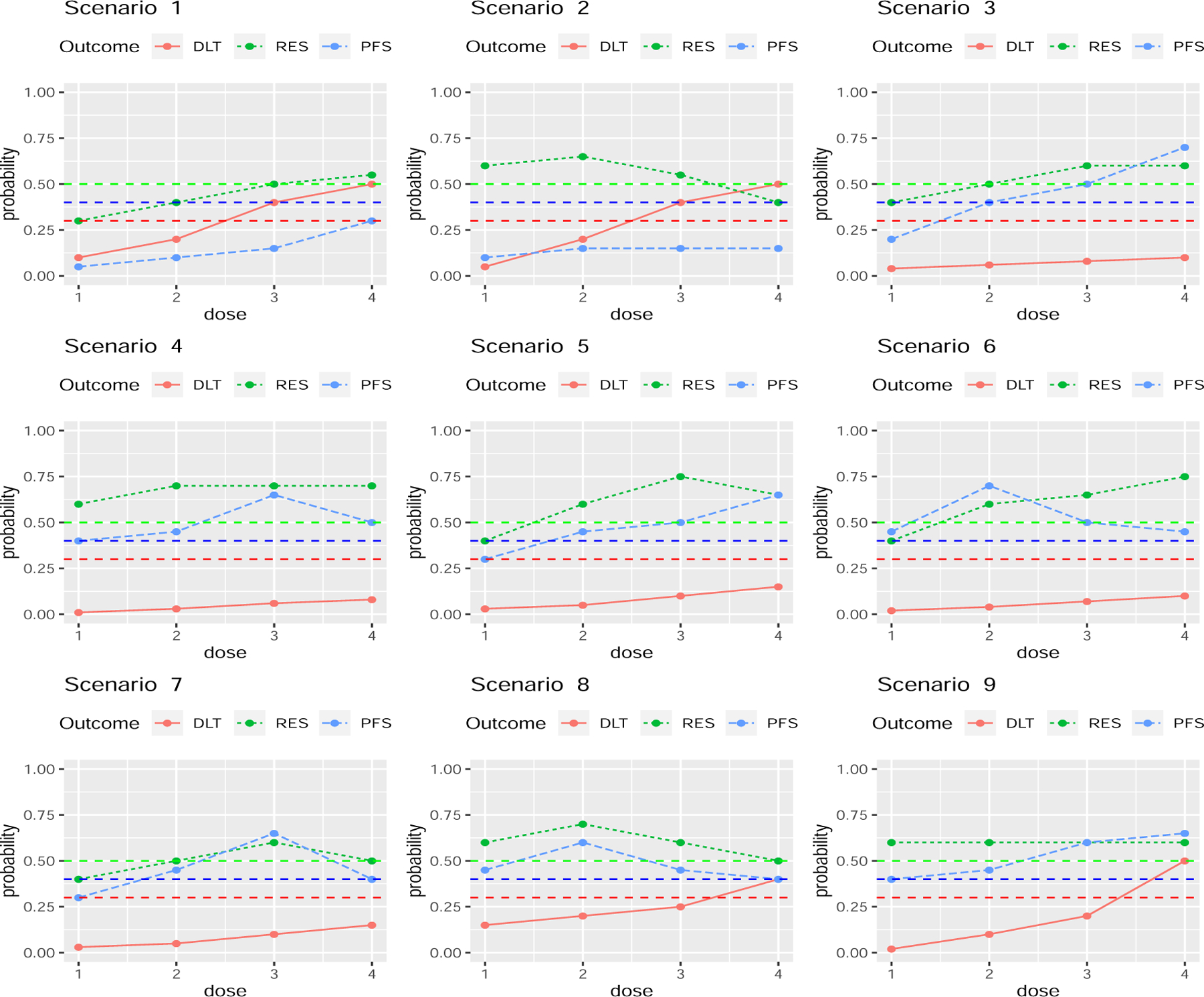
Dose-outcome curves for the scenarios in the simulation study. The red, green, and blue curves are ${\pi }_T^{true}\left(d_j\right)$, ${\pi }_R^{true}\left(d_j\right)$, and ${\xi }^{true}\left(d_j\right)=P{r}^{true}\left(Z>t_2-t_1|Z>0,d_j\right)$, respectively. The horizontal lines show the fixed upper limit .30 for π_T(d_j) and fixed lower limit .50 for π_R(d_j) in the dose admissibility rules, and the fixed lower limit 0.40 for ξ(d_j) for long-term success probability.

Table 2 summaries OCs of the Gen I-II, Conv 1, and Conv 2 designs, including dose selection percentages, mean number of patients treated at each dose, and mean overall sample size. The number tabled under “dose 0” is the percentage of trials stopped early with no dose selected. A summary statistic to evaluate performance by comparing the selected optimal dose to the truly optimal dose is $R\left(d^{sel,\xi }\right)=\xi \left(d^{sel,\xi }\right)/\xi \left(d^{opt,\xi }\right.$, which has domain [0, 1], with $R\left(d^{sel,\xi }\right)=1$ corresponding to always selecting the dose that maximizes long term treatment success probability. Using $R\left(d^{opt,\xi }\right)$ rather than only the empirical probability of selecting $d^{opt,\xi }$ to quantify how well a method behaves is useful in scenarios where two or more doses have $\xi {\left(d\right)}^{true}$ close to $\xi \left(d^{opt,\xi }\right)$, so choosing a nearly optimal dose is a good decision.

Table 2:

Selection % and mean number of patients treated at each dose level, mean sample size, and $R=\xi \left(d^{sel,\xi }\right)/\xi \left(d^{opt,\xi }\right)$ under the Gen I-II, Conv 1 and Conv 2 designs. The true long term success probability at d_j is ${\xi }^{true}\left(d_j\right)=P{r}^{true}\left(Z>5|Y_R^{\prime }>0,d_j\right)$. Boldface indicates results for the true optimal decision. The numbers in the brackets indicate the Monte Carlo simulation standard errors.

		Dose levels					Sample
Designs		0*	1	2	3	4	size	R %
Scenario 1
	${\pi }_T^{true}\left(d_j\right)$		0.10	0.20	0.40	0.50
	${\pi }_R^{true}\left(d_j\right)$		0.30	0.40	0.50	0.55
	${\overline{U}}^{true}\left(d_j\right)$		59.1	62.5	60.9	59.9
	${\xi }^{true}\left(d_j\right)$		0.05	0.1	0.15	0.3
Gen I-II	Selection %	93.5(0.3)	0	0.50	2.6	3.3	35.6	NA
	Patients		9.5	13.5	8.8	3.7
Conv 1	Selection %	56.2(0.7)	6.5	22.6	12.4	2.2	34.9	NA
	Patients		9.4	13.2	8.7	3.6
Conv 2	Selection %	57.7(0.7)	5.6	22.1	12.4	2.2	35.4	NA
	Patients		9.4	13.4	8.8	3.7
Scenario 2
	${\pi }_T^{true}\left(d_j\right)$		0.05	0.20	0.40	0.50
	${\pi }_R^{true}\left(d_j\right)$		0.60	0.65	0.55	0.40
	${\overline{U}}^{true}\left(d_j\right)$		76.7	68.0	54.0	40.4
	${\xi }^{true}\left(d_j\right)$		0.1	0.15	0.15	0.15
Gen I-II	Selection %	83.8(0.5)	2.3	9.6	4.1	0.2	48.2	NA
	Patients		21.5	16.4	7.4	2.8
Conv 1	Selection %	3.2(0.2)	73.3	22.4	1.1	0	46.9	NA
	Patients		21.2	15.9	7.0	2.8
Conv 2	Selection %	3.1(0.2)	73.2	22.8	0.9	0	48.2	NA
	Patients		21.4	16.6	7.3	2.9
Scenario 3
	${\pi }_T^{true}\left(d_j\right)$		0.04	0.06	0.08	0.10
	${\pi }_R^{true}\left(d_j\right)$		0.40	0.50	0.60	0.60
	${\overline{U}}^{true}\left(d_j\right)$		61.2	67.0	74.2	75.0
	${\xi }^{true}\left(d_j\right)$		0.20	0.40	0.50	0.70
Gen I-II	Selection %	2.9	0.3	7.0	19.3	70.5(0.6)	52.7	91.0
	Patients		10.6	13.0	14.9	14.3
Conv 1	Selection %	2.2	4.6	13.5	39.7	39.9(0.7)	47.4	79.1
	Patients		9.6	11.7	13.3	12.7
Conv 2	Selection %	2.2	3.6	13.2	40.2	40.8(0.7)	52.8	79.9
	Patients		10.5	13.1	14.9	14.3
Scenario 4
	${\pi }_T^{true}\left(d_j\right)$		0.01	0.03	0.06	0.08
	${\pi }_R^{true}\left(d_j\right)$		0.6	0.7	0.70	0.70
	${\overline{U}}^{true}\left(d_j\right)$		72.1	80.9	81.3	80.6
	${\xi }^{true}\left(d_j\right)$		0.4	0.45	0.65	0.50
Gen I-II	Selection %	0.1	4.3	9.2	69.1(0.7)	17.2	58.1	91.5
	Patients		13.9	15.1	14.8	14.4
Conv 1	Selection %	0	8.7	33.0	31.1(0.7)	27.7	48.0	80.1
	Patients		11.5	12.7	12.1	11.6
Conv 2	Selection %	0.1	7.0	33.2	32.3(0.7)	27.3	58.1	80.6
	Patients		13.8	15.3	14.8	14.1
Scenario 5
	${\pi }_T^{true}\left(d_j\right)$		0.03	0.05	0.1	0.15
	${\pi }_R^{true}\left(d_j\right)$		0.4	0.6	0.75	0.65
	${\overline{U}}^{true}\left(d_j\right)$		63.1	75.2	82.3	72.7
	${\xi }^{true}\left(d_j\right)$		0.3	0.45	0.5	0.65
Gen I-II	Selection %	1.2	1.4	14.2	24.1	59.1(0.7)	54.3	89.1
	Patients		10.5	14.7	15.8	13.3
Conv 1	Selection %	1.0	2.2	22.8	61.3	12.8(0.5)	47.7	77.1
	Patients		9.1	13.0	14.1	11.4
Conv 2	Selection %	1.1	1.6	20.1	64.6	12.6(0.5)	54.3	77.5
	Patients		10.2	14.9	16.2	13.1
Scenario 6
	${\pi }_T^{true}\left(d_j\right)$		0.02	0.04	0.07	0.10
	${\pi }_R^{true}\left(d_j\right)$		0.4	0.60	0.65	0.75
	${\overline{U}}^{true}\left(d_j\right)$		54.4	72.6	72.5	77.8
	${\xi }^{true}\left(d_j\right)$		0.45	0.70	0.5	0.45
Gen I-II	Selection %	0.6	5.4	68.4(0.7)	15.7	9.8	54.3	90.0
	Patients		10.0	14.4	14.7	15.2
Conv 1	Selection %	0.9	1.4	25.1(0.6)	25.3	47.2	47.7	75.2
	Patients		8.8	12.9	12.8	13.2
Conv 2	Selection %	1.1	1.0	23.9(0.6)	23.6	50.5	54.2	74.6
	Patients		9.9	14.6	14.5	15.1
Scenario 7
	${\pi }_T^{true}\left(d_j\right)$		0.03	0.05	0.1	0.15
	${\pi }_R^{true}\left(d_j\right)$		0.4	0.5	0.6	0.50
	${\overline{U}}^{true}\left(d_j\right)$		66.1	70.3	73.5	68.6
	${\xi }^{true}\left(d_j\right)$		0.3	0.45	0.65	0.4
Gen I-II	Selection %	3.3	2.0	15.0	70.9(0.6)	8.8	52.2	90.6
	Patients		11.2	13.7	15.1	12.1
Conv 1	Selection %	2.8	11.4	26.2	42.9(0.7)	16.6	47.4	78.9
	Patients		10.1	12.5	14.0	10.7
Conv 2	Selection %	2.8	10.2	26.2	44.6(0.7)	16.3	52.2	79.7
	Patients		11.1	13.9	15.3	11.8
Scenario 8
	${\pi }_T^{true}\left(d_j\right)$		0.15	0.20	0.25	0.40
	${\pi }_R^{true}\left(d_j\right)$		0.6	0.70	0.6	0.50
	${\overline{U}}^{true}\left(d_j\right)$		71.8	77.8	68.5	56.4
	${\xi }^{true}\left(d_j\right)$		0.45	0.60	0.45	0.40
Gen I-II	Selection %	9.1	23.4	56.9(0.7)	9.0	1.6	47.7	90.5
	Patients		17.7	14.8	9.9	5.30
Conv 1	Selection %	9.1	29.3	52.9(0.7)	8.2	0.5	44.2	89.5
	Patients		16.5	14.1	9.0	4.60
Conv 2	Selection %	9.0	28.3	54.0(0.7)	8.4	0.3	47.7	89.8
	Patients		17.4	15.2	10.0	5.10
Scenario 9
	${\pi }_T^{true}\left(d_j\right)$		0.02	0.1	0.2	0.5
	${\pi }_R^{true}\left(d_j\right)$		0.6	0.6	0.6	0.6
	${\overline{U}}^{true}\left(d_j\right)$		76.3	73.5	70.2	60.4
	${\xi }^{true}\left(d_j\right)$		0.4	0.45	0.6	0.65
Gen I-II	Selection %	1.3	18.2	22.5	51.2(0.7)	6.8	51.6	88.7
	Patients		17.2	15.6	12.8	5.9
Conv 1	Selection %	0.9	50.6	31.0	16.5(0.5)	1.0	47.7	75.2
	Patients		16.1	14.4	11.9	5.2
Conv 2	Selection %	1.1	49.6	31.8	16.9(0.5)	0.6	51.5	75.2
	Patients		17.2	15.4	13.1	5.7

^*The number under d = 0 is the percentage of trials terminated early with no dose is selected.

Scenarios 1 and 2 are null cases where no dose has both acceptably low ${\pi }_T^{true}\left(d_j\right)$ and acceptably high $\xi {\left(d\right)}^{true}$. In scenario 1, the Gen I-II design terminates the trial early 93.5% of the time compared to 56.2% and 57.7% for Conv 1 and Conv 2. In scenario 2, the Gen I-II design terminates the trial early 83.8% of the time. Because d₁ and d₂ both have large ${\pi }_R^{true}\left(d_j\right)$ and the conventional designs ignore Z, both conventional designs have only about a 3% chance of stopping early, and a 73% chance of incorrectly selecting d₁ as optimal. Scenario 2 illustrates the advantage that the Gen I-II design includes an admissibility requirement defined in terms of $\xi {\left(d\right)}^{true}$, while the conventional designs do not, and consequently they both have a high risk of selecting a dose with a low long term success rate. In scenarios 1 and 2, because no truly optimal dose exists, R is undefined.

In scenarios 3 and 4, multiple doses are nearly optimal in terms of ${\overline{U}}^{true}\left(d_j\right)$ based on Y, but only one dose is optimal based on the long-term criterion ${\xi }^{true}\left(d_j\right)$. In scenario 3, d₃ and d₄ have similar mean utilities near 75, while d₄ is truly optimal with highest ${\xi }^{true}\left(d_4\right)=0.70$, compared to ${\xi }^{true}\left(d_3\right)=0.50$. In scenario 4, d₂, d₃ and d₄ have similar mean utilities ${\overline{U}}^{true}\left(d_j\right)$ near 81, but d₃ is truly optimal with ${\xi }^{true}\left(d_3\right)=0.65$, compared to ${\xi }^{true}\left(d_2\right)=.45$ and ${\xi }^{true}\left(d_4\right)=.50$. The Gen I-II design has a 69.1% chance of correctly selecting d₃ in scenario 3, whereas the Conv 1 and Conv 2 designs have 31% and 32% chances of selecting d₃, and are about as likely to select d₂ or d₄, because both conventional designs ignore Z.

In scenarios 5 and 6, the truly optimal dose in terms of ${\xi }^{true}\left(d_j\right)$ and the dose with highest mean utility ${\overline{U}}^{true}\left(d_j\right)$ differ. In scenario 5, d₄ is truly optimal with the highest ${\xi }^{true}\left(d_4\right)=0.65$, whereas d₃ has the highest mean utility ${\overline{U}}^{true}\left(d_3\right)=82.3$. In scenario 6, d₂ is truly optimal with the highest ${\xi }^{true}\left(d_2\right)=0.70$, whereas d₄ has highest mean utility ${\overline{U}}^{true}\left(d_4\right)=77.8$. The Conv 1 and Conv 2 designs both have over a 60% chance of incorrectly selecting d₃ as optimal in scenario 5, about a 50% chance of incorrectly selecting d₄ as optimal in scenario 6, and both have below 15% and around 25% chances of correct optimal dose selection in scenarios 5 and 6. In contrast, the Gen I-II design has correct dose selection rates 59.1% in scenario 5 and 68.4% in scenario 6. In scenarios 7 and 8, the truly optimal dose and the dose with highest mean utility are identical. The Gen I-II design still outperforms the Conv 1 and Conv 2 designs, with a 25% higher correct optimal dose selection percentage in scenario 7. In scenario 8, the Gen-II design and the Conv 2 have similar correct optimal dose selection percentages of 56.9% and 54.0%, respectively. In scenario 9, ${\pi }_R{\left(d\right)}^{true}$ is flat and ${\pi }_T{\left(d\right)}^{true}$ increases with d, so the mean utility ${\overline{U}}^{true}\left(d_j\right)$ decreases monotonically with d, but the truly optimal dose in terms of ${\xi }^{true}\left(d_j\right)$ is d₃. In this case, the Gen-I-II design outperforms both Conv 1 and Conv 2, with about a 35% higher correct selection percentage.

In summary, in all scenarios, the Gen I-II design outperforms the conventional phase I-II designs substantially, with the highest R, that is at least 10% higher in each of scenarios 3 – 7. The three designs have similar patient allocation distributions, essentially because all designs allocate patients based on short-term outcomes, while Z is only used in the final optimal dose selection of the Gen I-II design.

We performed additional sensitivity analyses to explore several other aspects of the Gen I-II design. The results are summarized in the online supporting information. Table S1 summarizes the effects of including AR in stage 2. The design “with AR” is the Gen I-II design that allocates n₁ = 15 patients for the stage 1 and n₂ = 33 patients for stage 2 with AR; “without AR” is a modified Gen I-II design that combines stages 1 and 2, does not include AR, and allocates up to 48 patients with dose-finding done to maximize $u\left(d_j,{𝓓}_n\right)$ for all cohorts. Table S1 shows that, compared to the original “with AR” version of Gen I-II, the “without AR” version has substantially inflated sample sizes, with at most a mild gain of ≤ 5% in true optimal dose selection percentage. This shows that AR is a very useful component of the Gen I-II design that provides a large savings in sample size.

Recall that we fixed $\rho =0.70$ for defining a candidate dose set. Table S2 summarizes the OCs of the Gen I-II design for values of ρ ranging from 0.60 to 0.90. The results indicate that larger ρ is more favorable under the null scenarios 1 and 2, while smaller ρ is more favorable when a truly optimal dose exists, in scenarios 3 – 9. In practice, ρ should be chosen, based on preliminary simulations, to accommodate the application at hand.

Table S3 shows effects of changing patient allocation between stages 2 and 3. Given the values (n₂, N(d)) = (33,15) used in Table 2, we considered the two alternative pairs, (39,9) and (27,21). The results show that the allocation (33,15) and the alternative (39, 9) give very similar design performances, and that both give better OCs compared to (27,21) in terms of the tradeoff between correct true optimal dose selection percentage and sample size.

6. Discussion

By using data on duration of response, the Gen I-II design addresses an important problem with conventional phase I-II methods. The design is modular, since Y can be any ordinal early outcomes used by a phase I-II design, and any criterion $\varphi \left(d,\mathit{\theta }\right)$ can be used for stages 1 and 2. Thus, a Gen I-II design can be tailored to accommodate the particular clinical setting at hand. The Gen I-II design is practical in settings where investigators plan to follow patients long enough to assess response duration, which commonly is done in oncology trials. The main additional requirement is the sample of patients randomized among candidate doses in stage 3. Our simulations showed that about 15 more patients per candidate dose gives a reliable design. While we have investigated a utility-based Gen I-II design with a simple Bayesian model, the large advantages over conventional designs in our simulations suggest that other Gen I-II designs also will provide a large benefit over conventional designs.

Guo and Yuan [32] proposed a dose-ranging approach to optimizing dose (DROID) for oncology drug development. The Gen I-II design and DROID design share some high-level design strategies, including identifying an admissible dose set based on short-term endpoints, randomizing patients within the admissible dose set, and using both short-term and long-term endpoints for logistical convenience and identifying an optimal dose. However, they focus on different clinical settings. DROID considers binary toxicity and a continuous surrogate efficacy endpoint, e.g. pharmacodynamics, whereas Gen I-II considers early phase I-II toxicity and efficacy endpoints and a long term event time endpoint. This difference requires very different dose-outcome models. Stages 1 and 2 of a Gen I-II design follow the phase I-II paradigm [12], while DROID identifies both a minimal active dose (MAD) and MTD. The randomized portion of the DROID design, used for inference and decision making, does conventional dose-ranging, whereas stage 3 of the Gen I-II design is similar to a multi-arm randomized trial and identifies the dose with largest response duration.

A caveat is that, in settings using survival time rather than response duration to define long term treatment success, a Gen I-II design’s behavior wil depend on relationships between Y and survival time. This is a complex issue involving persistence of biological treatment effects over time, and effects of salvage therapy given at relapse on subsequent survival. How the Gen I-II paradigm behaves compared to conventional phase I-II designs in such settings is an important area for future research. R code for implementing the Gen I-II design is available from https://github.com/yongzang2020.

Data availability statement

Data sharing is not applicable to this paper as all data in this article are computer simulated.

References

- [1].Neelapu SS, Locke FL, Bartlett NL, et al. (2017) Axicabtagene Ciloleucel CAR T-Cell therapy in refractory large B-Cell lymphoma. N Engl J Med, 377, 2531–2544. [DOI] [PMC free article] [PubMed] [Google Scholar]
- [2].Liu E, Marin D, Banerjee P et al. (2020) Use of CAR-transduced natural killer cells in CD19-positive lymphoid tumors. N Engl J Med, 382, 545–553. [DOI] [PMC free article] [PubMed] [Google Scholar]
- [3].Thall PF and Cook JD (2004). Dose-Finding Based on Efficacy–Toxicity Trade-Offs. Biometrics 60, 684–693. [DOI] [PubMed] [Google Scholar]
- [4].Lee J, Thall PF and Rezvani K (2019). Optimizing natural killer cell doses for heterogeneous cancer patients on the basis of multiple event times. Journal of the Royal Statistical Society, Series C 68, 462–474. [DOI] [PMC free article] [PubMed] [Google Scholar]
- [5].Liu S, Guo B and Yuan Y (2018). A Bayesian phase I/II design for immunotherapy trials. Journal of the American Statistical Association, 113, 1016–1027. [DOI] [PMC free article] [PubMed] [Google Scholar]
- [6].O’Quigley J, Pepe M, Fisher L. (1990) Continual reassessment method: a practical design for phase 1 clinical trials in cancer. Biometrics, 46, 3348. [PubMed] [Google Scholar]
- [7].Babb J, Rogatko A, and Zacks S (1998). Cancer phase I clinical trials: Efficient dose escalation with overdose control. Statistics in Medicine 17 1103–1120. [DOI] [PubMed] [Google Scholar]
- [8].Liu S, Yuan Y. (2015) Bayesian optimal interval designs for phase I clinical trials. Journal of the Royal Statistical Society: Series C: Applied Statistics, 64, 507523. [Google Scholar]
- [9].Chu Y, Pan H, and Yuan Y (2016) Adaptive dose modification for phase I clinical trials. Statistics in Medicine 35, 3497–3508. [DOI] [PubMed] [Google Scholar]
- [10].Braun TM (2002). The bivariate continual reassessment method: Extending the CRM to phase I trials of two competing outcomes. Controlled Clinical Trials 23, 240–256. [DOI] [PubMed] [Google Scholar]
- [11].Zhang W, Sargent DJ and Mandrekar S (2006). An adaptive dose-finding design incorporating both toxicity and efficacy. Statistics in Medicine 25, 2365–2383. [DOI] [PubMed] [Google Scholar]
- [12].Yuan Y, Nguyen HQ, Thall PF (2016). Bayesian Designs for Phase I-II Clinical Trials Chapman & Hall/CRC: New York. [Google Scholar]
- [13].Zang Y and Lee JJ (2017). A robust two-stage design identifying the optimal biological dose for phase I/II clinical trials. Statistics in Medicine, 36, 27–42. [DOI] [PMC free article] [PubMed] [Google Scholar]
- [14].Guo B and Yuan Y (2017). Bayesian phase I/II biomarker-based dose finding for precision medicine with molecularly targeted agents. Journal of the American Statistical Association, 112, 508–520. [DOI] [PMC free article] [PubMed] [Google Scholar]
- [15].Zhou Y, Lee JJ, Yuan Y. (2019) A utility-based Bayesian optimal interval (U-BOIN) phase I/II design to identify the optimal biological dose for targeted and immune therapies. Statistics in Medine 38(28):5299–5316. [DOI] [PMC free article] [PubMed] [Google Scholar]
- [16].Lin R, Zhou Y, Yan F, Li D, Yuan Y. (2020) BOIN12: Bayesian Optimal Interval Phase I/II Trial Design for Utility-Based Dose Finding in Immunotherapy and Targeted Therapies. JCO Precision Oncology 4: 1393–1402. [DOI] [PMC free article] [PubMed] [Google Scholar]
- [17].Thall PF and Nguyen HQ (2012). Adaptive randomization to improve utility-based dose-finding with bivariate ordinal outcomes. Journal of Biopharmaceutical Statistics 22, 785–801. [DOI] [PMC free article] [PubMed] [Google Scholar]
- [18].Zhang Y, Cao S, Zhang C, Jin IH and Zang Y (2021). A Bayesian adaptive phase I/II clinical trial design with late-onset competing risk outcomes. Biometrics, 77: 796–808. [DOI] [PMC free article] [PubMed] [Google Scholar]
- [19].Zhang Y and Zang Y (2021). CWL: A conditional weighted likelihood method to account for the delayed joint toxicity-efficacy outcomes for phase I/II clinical trials. Statistical Methods in Medical Research, 30: 892–903. [DOI] [PubMed] [Google Scholar]
- [20].Lee J, Thall PF and Msaouel P (2020). A phase I-II design based on periodic and continuous monitoring of ordinal disease severity and the times to toxicity and death. Statistics in Medicine 39, 2035–2050. [DOI] [PMC free article] [PubMed] [Google Scholar]
- [22].Jin IH, Liu S, Thall PF and Yuan Y (2014). Using data augmentation to facilitate conduct of phase I–II clinical trials with delayed outcomes. Journal of the American Statistical Association 109, 525–536. [DOI] [PMC free article] [PubMed] [Google Scholar]
- [23].Al-Atrash G, Saberian C, Bassett R, Thall PF, Kebriaei P, et al. (2022). Vorinostat combined with busulfan, fludarabine, and clofarabine conditioning regimen for allogeneic hematopoietic cell transplantation in patients with acute leukemia: long-term study outcomes. Transplantation and Cellular Therapy 28, 501.e1–501.e7. [DOI] [PubMed] [Google Scholar]
- [24].Tseng YD, Chen YH, Catalano PJ and Ng A (2015). Rates and durability of response to salvage radiation therapy among patients with refractory or relapsed aggressive non-hodgkin lymphoma. International J Radiation Oncology, Biology, Physics 91, 223–231. [DOI] [PubMed] [Google Scholar]
- [25].Dazzi F, Szydlo RM, Cross NC and et al. (2000). Durability of responses following donor lymphocyte infusions for patients who relapse after allogeneic stem cell transplantation for chronic myeloid leukemia. Blood 15, 2712–2716. [PubMed] [Google Scholar]
- [26].Yan F, Thall PF, Lu KH, Gilbert MR and Yuan Y (2018). Phase I-II clinical trial design: A state-of-the-art paradigm for dose finding with novel agents. Annals of Oncology 29, 694–699. [DOI] [PMC free article] [PubMed] [Google Scholar]
- [27].Gauthier J, Yuan Y and Thall PF (2019). Bayesian phase 1/2 trial designs and cellular immunotherapies: a practical primer. Cell and Gene Therapy Insights 5, 1483–1495. [Google Scholar]
- [28].Anderson JR, Cain KC and Gelber RD (1983). Analysis of survival by tumor response. Journal of Clinical Oncology 1, 710–719. [DOI] [PubMed] [Google Scholar]
- [29].Simon RM and Makuch RW (1984). A non-parametric graphical representation of the relationship between survival and the occurrence of an event: Application to responder versus non-responder bias. Statistics in Medicine 3, 35–44. [DOI] [PubMed] [Google Scholar]
- [30].Buyse M and Piedbois P (1996). One the relationship between response to treatment and survival time. Statistics in Medicine 15, 2797–2812. [DOI] [PubMed] [Google Scholar]
- [31].Fleming TR and Powers JH (2012). Biomarkers and surrogate endpoints in clinical trials. Statistics in Medicine 31, 2973–2984. [DOI] [PMC free article] [PubMed] [Google Scholar]
- [32].Guo B and Yuan Y (2023). DROID: Dose-ranging Approach to Optimizing Dose in Oncology Drug Development. Biometrics, to appear [DOI] [PMC free article] [PubMed] [Google Scholar]
- [33].Thall and Russell (1998). A strategy for dose-finding and safety monitoring based on efficacy and adverse outcomes in phase I/II clinical trials. Biometrics 54, 251–264. [PubMed] [Google Scholar]
- [34].Thall PF, Herrick R, Nguyen HQ, Venier JJ and Norris JC (2014). Using effective sample size for prior calibration in Bayesian phase I-II dose-finding. Clinical Trials 11, 251–264. [DOI] [PMC free article] [PubMed] [Google Scholar]
- [35].Thall PF, Szabo A, Nguyen HQ, Amlie-Lefond CM and Zaidat OO (2011). Optimizing the concentration and bolus of a drug delivered by continuous infusion. Biometrics 67, 1638–1646. [DOI] [PMC free article] [PubMed] [Google Scholar]
- [36].Murray T, Thall P, Yuan Y, McAvoy S and Gomez D (2017) Robust treatment comparison based on utilities of semi-competing risks in non-small-cell lung cancer. Journal of the American Statistical Association, 112, 11–23. [DOI] [PMC free article] [PubMed] [Google Scholar]
- [37].Cheung YK and Chappell R. (2000) Sequential designs for phase I clinical trials with late-onset toxicities. Biometrics 56, 1177–1182. [DOI] [PubMed] [Google Scholar]
Associated Data
This section collects any data citations, data availability statements, or supplementary materials included in this article.
Supplementary Materials