Predicting Visual Field Worsening with Longitudinal Optical Coherence Tomography Data Using a Gated Transformer Network (OPHTHA-D-22-01964)s

Abstract

Purpose:

To identify visual field (VF) worsening from longitudinal optical coherence tomography (OCT) data using a Gated Transformer Network (GTN), and to examine how GTN performance varies for different definitions of visual field worsening and different stages of glaucoma severity at baseline.

Participants:

A total of 4,211 eyes (2,666 patients) followed at the Johns Hopkins Wilmer Eye Institute with at least five reliable VFs and one reliable OCT within one year of each reliable VF.

Design:

Retrospective longitudinal cohort study.

Methods:

For each eye, we used three trend-based methods (MD, VFI, and PLR slope) and three event-based methods (GPA, CIGTS, and AGIS) to define VF worsening. Additionally, we created an algorithm, called M6, that classifies an eye as worsening if 4 or more of the 6 aforementioned methods classifies the eye as worsening. Using these 7 reference standards for VF worsening, we trained 7 GTNs that accepts a series of at least 5 as input OCT scans and provides as output a probability of VF worsening. GTN performance was compared to non-deep learning models with the same serial OCT input from previous studies — linear mixed effects models (MEM) and naïve Bayes classifiers (NBC) — using the same training sets and reference standards as for the GTN. The effect of glaucoma severity at baseline VF on GTN performance was also investigated through stratified analysis.

Main Outcome Measures:

Area under the receiver operating characteristic curve (AUC) and F1 score.

Results:

The M6 algorithm labeled 63 eyes (1.50%) as worsening. The GTN achieved an AUC (95% CI) of 0.97 (0.88, 1.00) when trained with M6. GTNs trained and optimized with the other 6 reference standards had AUC ranging from 0.78 (MD slope) to 0.89 (AGIS). The 7 GTNs outperformed all 7 MEMs and all 7 NBCs accordingly. GTN performance was worse for eyes with more severe glaucoma at baseline.

Conclusions:

GTN models trained with OCT data may be used to identify VF worsening. After further validation, implementing such models in clinical practice may allow us to track functional worsening of glaucoma with less onerous structural testing.

Introduction

Glaucoma is the leading cause of irreversible blindness worldwide^1,2. Visual fields (VF) and optical coherence tomography (OCT) are commonly used to diagnose glaucoma and track its worsening^3,4 VFs measure functional deficits, and OCT measure structural deficits by quantifying retinal nerve fiber layer (RNFL) thickness. Previous work has shown that structural deficits measured by OCT (decreased RNFL thickness) typically precede functional deficits measured in VF (loss of sensitivity globally or locally)⁵. While visual function is more important to patient quality of life than structural measurements on OCT^6,7, measuring function with VF testing can be cumbersome due to the requirement for patient cooperation/attention and rather lengthy test time (approximately 6 minutes per eye on average for SITA Standard testing)^8,9. Lack of cooperation/attention may lead to VF results that are not reliable¹⁰ and therefore hinder the ability to track functional change over time. OCT of the optic nerve head can be obtained without significant cooperation, and acquisition time is on the order of seconds rather than minutes. Therefore, if OCT can be used to identify VF change over time, clinicians may be able to track the functional impact of glaucoma with much less onerous testing.

Prior studies developed mixed effects models (MEM) and other machine learning models to identify VF worsening using longitudinal OCT measurements as inputs^11,12. In these studies, VF worsening was defined using pointwise linear regression (PLR) or Guided Progression Analysis (GPA). The MEM attempted to predict VF worsening by using linear regression of serial OCT measures such as average RNFL thicknesses, clockwise RNFL thickness, and rim area as input¹¹. Another recent study applied a naïve Bayes classifier (NBC) to longitudinal RNFL thickness measurements and demographics to predict VF worsening¹². These MEM and NBC achieved areas under the receiver operating characteristic curves (AUC) of between 0.60 and 0.85 for predicting VF worsening using OCT data.

In this work, we aim to improve on prior results by using a Gated Transformer Network (GTN) which is a recent innovation in deep learning that specializes in multivariate time series classification¹³. GTNs have haven been successfully employed in 13 different multivariate time series datasets, outperforming all previous benchmarks¹³. As our serial OCT/VF dataset is a multivariate time series, we assess how well a GTN can utilize serial OCT data to predict VF worsening. Additionally, we assess how model performance changes for different definitions of VF worsening (trend and event-based methods), since this allows us to investigate if the GTN is capable of learning multiple definitions of VF worsening and if OCT data is better at detecting one type of VF worsening than the others. Finally, we assess how the GTN performs across various levels of glaucoma severity.

Methods

This study was reviewed and approved by the Johns Hopkins University School of Medicine Institutional Review Board and adhered to the tenets of the Declaration of Helsinki.

Data Collection & Inclusion

We included eyes followed at the Johns Hopkins Wilmer Eye Institute for glaucoma related diagnoses (based on ICD codes captured in the electronic medical record) from April 2013 to July 2021 if they had five or more reliable VFs and one unique reliable OCT within one year (either direction) of each reliable VF. Using established criteria, we defined a VF as reliable if it had < 15% false positives, and either < 25% false negatives for suspect/mild/moderate glaucoma (MD ≥ −12 dB) or < 50% false negatives for severe glaucoma (MD < −12 dB)¹⁰. Glaucoma suspects had a normal glaucoma hemifield test (GHT) and a mean deviation (MD) value of less than −6 dB their initial VF test. We defined an OCT scan as reliable if signal strength was greater than 6 and average, superior quadrant, and inferior quadrant RNFL thickness were all greater than 30 μm^14,15. The thickness floor was set to 30 microns as values below this level are likely representative of artifact or segmentation errors. All included eyes underwent VF testing using the SITA 24–2 on the Humphrey Field Analyzer (HFA), and retinal nerve fiber layer (RNFL) thickness was measured using CIRRUS HD-OCT (Zeiss, Dublin, CA). A flow diagram for inclusion and exclusion criteria is illustrated in Figure S1.

Determining Visual Field Worsening

There is currently no single widely-accepted standard to assess VF worsening. However, there are many methods that are commonly employed. We selected 6 such methods: three trend-based methods and three event-based algorithms, so that we can investigate if the GTN is capable of learning multiple definitions of VF worsening and if OCT data is better at detecting one type of VF worsening than the others. The trend-based methods are: rate of change in mean deviation (MD slope), rate of change in VF index (VFI slope), and rate of change estimated by Pointwise Linear Regression (PLR). The event-based algorithms are: Guided Progression Analysis (GPA), Advanced Glaucoma Intervention Study (AGIS) scoring system, and the Collaborative Initial Glaucoma Treatment Study (CIGTS) scoring system.

All three trend-based methods use linear regression. With MD slope, eyes are labeled as worsening if MD slope < −0.5 dB/year with p-value < 0.05. For VFI slope, eyes are worsening if VFI slope < −1.8%/year with p-value < 0.05¹⁶. For PLR, linear regression is performed on the total deviation values at each of the 52 test locations in the 24–2 test pattern across all VFs, and eyes are labeled as worsening if there are at least three test points with slope < −1 dB/year and p-value ≤ 0.01¹⁶.

GPA is a proprietary algorithm for measuring VF worsening^16,17 that compares pattern deviation values at each test point to the average of those values from the first two VFs. Test points that show statistically significant change as compared to the expected test-retest variability are identified by GPA. Since we did not have access to the test-retest variability database used by GPA, we determined thresholds at α = 0.05 using an empiric normative database from the University of Iowa. We also used total deviation instead of pattern deviation as recent studies suggest total deviation to be more sensitive at predicting VF worsening¹⁸. The result was a GPA-like algorithm that defines worsening if three or more test points worsen beyond the threshold level for three consecutive VFs compared to the first two VFs. For simplicity, we will refer to this GPA-like algorithm as “GPA”.

Unlike GPA, AGIS and CGITS are not proprietary. AGIS scores each VF on a 0–20 scale based on the number of defects in the nasal, superior, and inferior hemifields of each VF using total deviation values^19,20. Each VF’s AGIS score then is compared to the score at baseline. Eyes with increasing AGIS scores at four or more test points over three consecutive VFs are labeled as worsening. CGITS also uses total deviation and calculates a 0–20 score based on the density and depth of defects across all VF test points²¹. To avoid misclassifying artifacts as defects, VFs that have multiple isolated defects receive a lower CGITS score than when there are clusters of test points with defects. Eyes with an increase of three or more CGITS scores over three consecutive VFs are labeled as worsening.

Each of the aforementioned 6 methods identifies VF worsening by focusing on a different aspect of the VF progression. To incorporate and balance these differences we created an algorithm that classifies an eye as worsening if 4 or more of the 6 methods (MD slope, VFI slope, PLR, GPA, AGIS, CIGTS) identify the eye as worsening — our “majority out of 6” algorithm (M6 for short).

In total, we have 7 methods (MD slope, VFI slope, PLR, GPA, AGIS, CIGTS, and M6). We used each method to define a reference standard and independently train seven different GTNs.

Model Development - Gated Transformer Networks (GTN)

The Transformer is a recent innovation in deep learning that achieves frontier performance in learning sequential data inputs by incorporating an attention mechanism^22–24. The Gated Transformer Network (GTN) merges two Transformers — a longitudinal Transformer and a cross-sectional Transformer — that learn different aspects of the data, and specializes in multivariate time series classification (Figure 2)¹³. For each input instance (i.e., a time-series of at least 5 OCT scans of an eye), the GTN passes data to two separate Transformers — the longitudinal Transformer discovers changes in the same feature across different time stamps (changes in average RNFL thickness over time), while the cross-sectional Transformer learns correlations between different features at the same time stamp (relationship between inferior RNFL thickness and superior RNFL thickness). These two Transformers are then combined with a gating layer before outputting the final probability of VF worsening. The input instances are not required to have the same number and frequency of OCT scans, and each input instance is composed of all available OCT scans (5 or more) of a unique eye. During training, the gating layer helps the GTN optimize the weights on the two Transformers. This architecture outperformed previous benchmarks on 13 different multivariate time-series datasets, demonstrating its generalizability¹³.

Figure 2 –

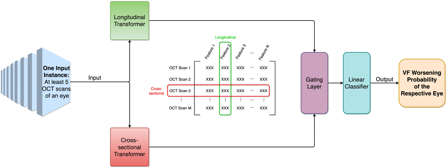
Gated Transformer Network (GTN) architecture. The GTN takes one input instance (i.e., serial OCT scans of an eye) and passes it to two separate Transformers (i.e., cross-sectional transformer and longitudinal transformer), which use attention mechanism to learn different aspects of the input data. The gating layer then incorporates learning results from both Transformers with different weights, and finally the GTN outputs the VF worsening probability of the respective eye.

We trained 7 GTNs with 7 different reference standards — one reference standard for VF progression per model. For each GTN, we input the model with demographics information and time-series OCT data for each eye. The model then outputs the probability of VF worsening for each eye. The demographics information included age, gender, and race, while the OCT data incorporated signal strength, RNFL thickness (clockwise channels and Garway-Heath Zones), average & vertical cup disc ratio, rim area, and cup volume. At a patient level, the whole input dataset was randomly split into training, validation, and testing subsets. We found the split that led to the highest F1 score by changing the size of the training set from 50% to 90% in steps of 5% while keeping an equal size for validation and testing. The result was 65%, 17.5%, 17.5% for training, validation, and testing respectively. GTNs were trained in PyTorch with optimized hyperparameters and with a batch size of 1024 for 500 epochs on the training dataset. After training, we optimized each GTN by selecting the model state that yields the highest F1 score on the validation dataset. To investigate the influence of demographic data on model performance, we also trained a separate GTN excluding demographic information (i.e., age, gender, and race) from the input features.

To evaluate model performance, we calculated AUC for the receiver operating characteristic (ROC) curve and its 95% CI using the Clopper-Pearson method²⁵. A Precision Recall curve was also generated. In addition, we calculated sensitivity, specificity, and Youden’s J-statistic²⁶ at the point where Youden’s J statistics (optimal threshold that balances sensitivity and specificity) was maximized. Precision and recall were calculated at the point where precision and recall were equally weighted using the F1 score. We compared our GTN to non-deep learning models used in previous studies — 7 different linear mixed effects models (MEM) and 7 naïve Bayes classifiers (NBC)^11,12 — by using the exact same training sets and reference standards for all models.

Results

Table 1 shows demographics and VF characteristics of the 4,211 eyes from 2,666 patients who satisfied our inclusion criteria — Figure S1 illustrates the inclusion-exclusion criteria. As previously stated in the Data Collection & Inclusion section, eyes were included as long as they had at least 5 reliable pairs of VF and OCT tests, regardless of the time between any of these paired tests. On average, the included eyes had 448.73 (240.05) days (SD) between their 1^st & 2^nd VF test and 1726.75 (454.15) days (SD) between their 1^st & 5^th VF tests. Similarly, the included eyes had 428.43 (225.03) days (SD) between their 1^st & 2^nd OCT tests and 1701.57 (431.33) days (SD) between their 1^st & 5^th OCT tests. 17 out of the 4,211 included eyes (0.40%) had 5 reliable pairs of OCT and VF tests within 1 year, and no eye had 5 pairs of OCT and VF tests over a period greater than 9 years.

Table 1.

Demographics and visual field characteristics of eyes included in this study. Abbreviations used: mean deviation (MD), pattern standard deviation (PSD), retinal nerve fiber layer (RNFL).

		Overall	M6 Worsening Eyes (n= 63)	M6 Stable Eyes (n= 4,148)
Demographics	Total number of eyes (# of patients)	4,211 (2,666)	63 (58)	4,148 (2,645)
	Mean Age at first VF (SD)	64.69 (11.84)	68.53 (11.82)	64.65 (11.82)
	# of Female (proportion)	1,569 (58.85%)	35 (60.34%)	1,555 (58.79%)
	# of White or Caucasian Patient (proportion)	1,513 (56.75%)	24 (41.38%)	1,505 (56.90%)
	# of Black or African American Patient (proportion)	935 (35.07%)	31 (53.45%)	925 (34.97%)
	# of Asian Patient (proportion)	107 (4.01%)	2 (3.45%)	105 (3.97%)
	# of Other or Unknown Patient (proportion)	111 (4.16%)	1 (1.72%)	110 (4.16%)
Glaucoma Severity at Baseline VF	# of Eyes with Mild Glaucoma at first VF (proportion)	3,685 (87.45%)	43 (68.25%)	3,639 (87.73%)
	# of Eyes with Moderate Glaucoma at first VF (proportion)	369 (8.76%)	16 (25.40%)	353 (8.51%)
	# of Eyes with Severe Glaucoma at first VF (proportion)	160 (3.80%)	4 (6.35%)	156 (3.76%)
VF Characteristics	Mean Baseline MD in dB (SD)	−2.55 (3.82)	−4.65 (3.83)	−2.52 (3.82)
	Mean Baseline PSD in dB (SD)	3.15 (2.83)	5.13 (3.34)	3.12 (2.81)
	Mean VF MD Slope in dB/year (SD)	−0.0798 (0.6634)	−1.70 (1.43)	−0.0741 (0.5998)
OCT Characteristics	Mean Baseline Cup Disc Ratio (SD)	0.63 (0.15)	0.70 (0.17)	0.63 (0.15)
	Mean Baseline Rim Area in mm2 (SD)	1.05 (0.26)	0.92 (0.25)	1.05 (0.26)
	Mean Baseline RNFL Thickness in ^m (SD)	80.47 (12.13)	74.41 (12.77)	80.56 (12.09)
	Mean RNFL Slope in ^m/year (SD)	−0.4118 (1.3795)	−1.0678 (2.5056)	−0.4069 (1.3493)

The M6 algorithm labeled 63 of these eyes as worsening. These worsening eyes had lower (worse) baseline MD, lower baseline RNFL thickness, and higher (worse) baseline pattern standard deviation (PSD) compared to stable eyes. When followed with VF and OCT over time, these worsening eyes showed lower MD slope per year, and lower RNFL thickness slope per year. Worsening eyes had older mean age at the first VF and were more likely to have severe glaucoma at the baseline VF. All comparisons above were statistically significant using Welch’s t-test with α = 0.05.

Figure 3 shows the agreement on worsening decisions by the three trend-based and three event-based algorithms used to construct M6. This UpSet plot shows the intersections of 6 different sets that define a Venn diagram. The MD slope algorithm identified the highest number of worsening eyes with 258 (6.13%) followed by CGITS with 227 (5.39%). PLR and AGIS identified the fewest worsening eyes with 112 (2.66%) eyes and 37 (0.88%) eyes, respectively. Figure 3 shows that the 6 reference standards demonstrate moderate agreement (Fleiss’ Kappa = 0.41) with each other, with only 10 eyes labeled as worsening by all 6 algorithms (right most column).

Figure 3 –

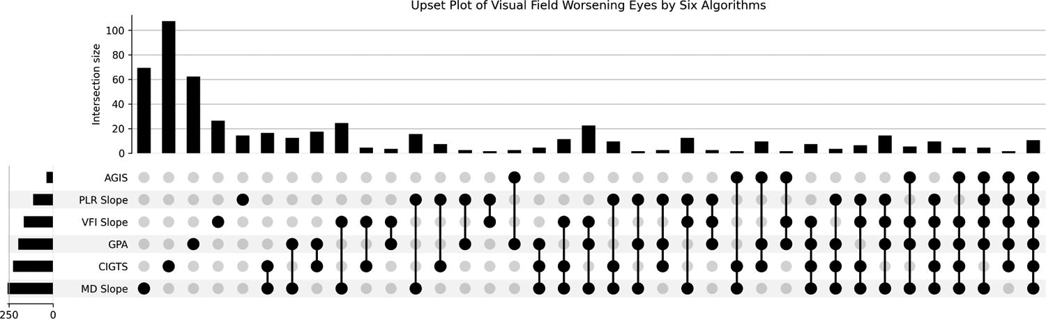
Agreement between the 6 reference standards: Mean Deviation rates of change (MD slope), Visual Field Index rates of change (VFI slope), Pointwise Linear Regression (PLR), Guided Progression Analysis (GPA), Advanced Glaucoma Intervention Study (AGIS), Collaborative Initial Glaucoma Treatment Study (CIGTS). Each column corresponds to a set, and bar charts on top show the size of the set. Each row corresponds to a possible intersection: the filled-in cells show which set is part of an intersection. When only one cell is filled, the height of the vertical bar on top represents the number of element only appeared in that set. The height of the horizontal bar represents the number of elements in the set. Bars with zero height are not shown.

Figure 4 shows performance of the GTN at predicting worsening based on 7 different labeling methods (MD slope, VFI slope, PLR, GPA, AGIS, CGITS, and M6) with the optimal split. The GTN trained with M6 labeling (blue curve) had the best AUC (95% CI) of 0.97 (0.88, 1.00). GTNs trained and optimized with the other 6 reference standards had AUC ranging from 0.78 (MD slope) to 0.89 (AGIS). The results of the PR curve are analogous to the ROC curve. The PR curve (and F1 scores) shows that the GPA-trained GTN has the highest precision with an equal recall weighting, followed by the M6-trained GTN. Figure S5 shows the representative true positive, false positive, true negative, and false negative cases of the M6-trained GTN, using a threshold determined by the Youden’s J statistics. The GTN trained without demographic features (i.e., age, gender, race) resulted in an AUC (95% CI) of 0.91 (0.76, 1.00) by the M6 reference standard.

Figure 4 –

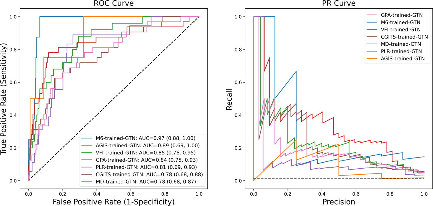
The Receiver Operating Characteristic (ROC) curves (left) and Precision Recall (PR) curves (right) of the Gated Transformer Network (GTN) trained with different reference standards.

More detailed model performance metrics are displayed in Table 2. Consistent with the ROC curve, Youden’s J statistic showed that the GTN trained with the M6 reference standard was the best predictor when sensitivity and specificity were equally weighted. With the PR curve, F1 scores showed that the GPA-trained GTN achieved the best balance between precision and recall.

Table 2 –

Comparison of GTN performance for the 7 reference standards: majority of 6 (M6), mean deviation rates of change (MD slope), visual field index rates of change (VFI slope), pointwise linear regression (PLR), guided progression analysis (GPA), advanced glaucoma intervention study (AGIS), collaborative initial glaucoma treatment study (CIGTS). Sensitivity, specificity, and Youden’s statistic were calculated at the point where Youden’s J statistic was maximized. Precision and recall were calculated at the point where precision and recall were equally weighted using the F1 score.

Reference Standard (Overall labeling frequency)	AUC (95% CI)	Youden’s J-Statistic (95% CI)	Sensitivity (95% CI)	Specificity (95% CI)	F1 Score (95% CI)	Precision (95% CI)	Recall (95% CI)
M6 (63/4,211 eyes)	0.97 (0.88, 1.00)	0.93 (0.81, 1.00)	1.00 (1.00, 1.00)	0.93 (0.82, 1.00)	0.36 (0.25, 0.48)	0.67 (0.54, 0.80)	0.25 (0.14, 0.36)
MD Slope (258/4,211 eyes)	0.78 (0.68, 0.87)	0.47 (0.34, 0.59)	0.63 (0.51, 0.75)	0.84 (0.75, 0.93)	0.26 (0.16, 0.35)	0.50 (0.46, 0.54)	0.13 (0.10, 0.15)
VFI Slope (166/4,211 eyes)	0.85 (0.76, 0.95)	0.59 (0.45, 0.73)	0.88 (0.79, 0.97)	0.71 (0.58, 0.83)	0.33 (0.21, 0.45)	0.22 (0.18, 0.26)	0.52 (0.48, 0.56)
PLR (112/4,211 eyes)	0.81 (0.72, 0.90)	0.63 (0.47, 0.79)	0.89 (0.79, 0.99)	0.74 (0.59, 0.89)	0.17 (0.11, 0.23)	0.10 (0.07, 0.12)	0.28 (0.24, 0.32)
GPA (196/4,211 eyes)	0.84 (0.75, 0.93)	0.66 (0.54, 0.79)	0.78 (0.67, 0.89)	0.88 (0.79, 0.97)	0.42 (0.24, 0.61)	0.42 (0.38, 0.46)	0.41 (0.37, 0.44)
AGIS (37/4,211 eyes)	0.89 (0.69, 1.00)	0.68 (0.40, 0.95)	1.00 (1.00, 1.00)	0.68 (0.40, 0.95)	0.31 (0.21, 0.41)	0.25 (0.20, 0.31)	0.25 (0.20, 0.31)
CGITS (227/4,211 eyes)	0.78 (0.68, 0.88)	0.47 (0.34, 0.60)	0.63 (0.50, 0.75)	0.85 (0.75, 0.94)	0.36 (0.24, 0.47)	0.39 (0.35, 0.43)	0.28 (0.24, 0.32)

The seven different GTNs outperformed all MEMs and NBCs. However, the MD-slope trained MEM had an AUC (95% CI) of 0.77 (0.74, 0.80), which was worse than that of the MD-slope-trained GTN but not statistically significant (p = 0.09). The M6-trained MEM and NBC had AUCs (95% CI) of 0.88 (0.84, 0.93) and 0.77 (0.7, 0.83) respectively. MEMs trained with the other 6 reference standards had AUCs (95% CI) ranging from 0.58 (0.53, 0.63) [CGITS] to 0.79 (0.76, 0.83) [VFI]. NBCs trained with the other 6 reference standards had AUCs (95% CI) ranging from 0.57 (0.53, 0.61) [CGITS] to 0.76 (0.67, 0.85) [AGIS]. Detailed MEM and NBC performances are outlined in Table S3.

Table 4 shows performance evaluation metrics for the GTN trained with the M6 reference standard as a function of glaucoma severity at baseline VF. For glaucoma suspects (eyes with MD < −6 dB and a normal GHT), the GTN model was able to make worsening judgments that perfectly matched the M6 algorithm (AUC = 1.00). On the other hand, the model performed worse when dealing with patients who had severe glaucoma (Welch’s t-test with p < 0.001).

Table 4 –

Test set performance of the M6-trained GTN, stratified by glaucoma severity. Sensitivity, specificity, and Youden’s statistic were calculated at the point where Youden’s J statistics was maximized. Precision and recall were calculated at the point where precision and recall were equally weighted using the F1 score. Abbreviations used: mean deviation (MD), glaucoma hemifield test (GHT), Area under the receiver operating characteristic curve (AUC).

Glaucoma Severity at Baseline	# of eyes (% of test set)	AUC (95% CI)	Youden’s J-Statistic	Sensitivity	Specificity	F1 Score	Precision	Recall
Initial MD > −6 with normal GHT (Suspect)	341 (47%)	1.0000 (0.9976, 1.0000)	1.00	1.00	1.00	1.00	1.00	1.00
Initial MD > −6 with abnormal GHT (Mild)	279 (39%)	0.9636 (0.8346, 1.0000)	0.92	1.00	0.92	0.40	0.12	0.75
Initial MD ≤ - 6 (Moderate/Severe)	99 (14%)	0.8750 (0.6235, 1.0000)	0.86	1.00	0.86	0.31	0.13	0.67

Discussion

In this study we used a state-of-the-art deep learning model architecture for time-series classification, the Gated Transformer Network, to predict the presence or absence of functional VF change from longitudinal structural OCT data. Our GTN learned to classify VF worsening using 7 different reference standards more accurately than prior models such as NBC and MEM. The 7 GTNs had varying performances based on the reference standard used. The GTN trained on a consensus definition of VF worsening (M6) had the highest AUC (95% CI) of 0.97 (0.88, 1.00). The average performance of event-based-trained GTNs was slightly better performance than that of the trend-based-trained GTNs. By testing the GTNs on datasets stratified by glaucoma severity, we found that GTNs based on OCT data identified VF worsening better for eyes with earlier stages of glaucoma.

Our GTNs demonstrated better performance at predicting VF worsening with serial OCT than prior work. A prior study used longitudinal OCT data to train an NBC on the PLR reference standard, and it achieved an AUC (95% CI) of 0.61 (0.46, 0.76)¹². To compare, we trained an NBC on the PLR reference standard using our dataset, resulting in an AUC (95% CI) of 0.65 (0.60, 0.70). Both results are significantly worse (p < 0.01) than for the PLR-trained GTN (AUC = 0.81). Another study trained a MEM with the GPA reference standard and achieved an AUC (95% CI) of 0.84 (0.77, 0.92)¹¹. For comparison, we also fit a MEM to our dataset and obtained an AUC (95% CI) of 0.79 (0.76, 0.83), which is significantly (p < 0.05) worse than the GTN trained on the same data and reference standard (AUC = 0.84). Detailed comparisons between NBC, MEM, and GTN are outlined in Table S3. One major advantage of the GTN comes from its double Transformer structure. Prior studies used longitudinal OCT information mainly by including the rate of change of each feature (e.g., RNFL thickness, rim area) as additional features^11,12. The GTN is able to more elaboratively investigate linear and non-linear correlations between features within each scan using the cross-sectional Transformer, while the longitudinal Transformer learns changes in features across time¹³. During training, the gating layer optimizes the GTN performance by learning to weigh the learning results from each Transformer differently. The GTN is therefore a “natural”¹³ architecture for learning relationships in multivariate time series data such as in our longitudinal OCT data.

Out of the 7 GTNs, the GTN trained with the M6 reference standard achieved the highest AUC of 0.97 (0.88, 1.00). This might be because by definition, the eyes that were labeled as worsening by M6 were also labeled by at least 4 out of the 6 reference standards, which means that these eyes were likely to exhibit more worsening patterns in their input OCT features than the eyes that weren’t labeled by the majority of reference standards. We also demonstrated that GTN is a better detector of VF change for all 7 types of reference standards that we used to identify VF worsening (Table S3). Figure 3 showed that the 6 trend-based and event-based reference standards exhibit weak agreement in defining VF worsening as shown in prior studies^16,27. Though it is not desirable for the 6 reference standards to be in such disagreement with each other our results show that the GTN is better at predicting all 7 reference standards compared to MEM) as well as NBC, suggesting better generalizability to future reference standards for measuring VF worsening.

On average, training the GTN with event-based methods (GPA, CGITS, AGIS) as reference standards resulted in slightly better performance than with trend-based methods (MD slope, VFI slope, PLR). The trend-based-trained GTNs had a mean AUC of 0.81 and mean F1 score of 0.25, while the event-based-trained GTNs had a mean AUC of 0.84 and mean F1 score of 0.36. This may be worsening in early glaucoma is often detected first with structure (on OCT) and concurrent early functional changes (on VF) are often detected with event based methods rather than trend based methods – suggesting that OCT may correlate better with event based methods^28,29.

Stratified by glaucoma severity at baseline VF, we found that GTN performance decreased as glaucoma severity increases. This is possibly due to many of the eyes with moderate/advanced glaucoma being closer to the RNFL thickness floor where it is more difficult for models to detect change over time³⁰. It might also because that eyes with mild baseline severity allows us to observe more RNFL change per VF progression endpoint. For example, eyes with severe glaucoma had a mean (SD) baseline average RNFL thickness of 69.59 (11.04) μm, which is closer to the RNFL thickness floor (57 μm)³¹ than the mean (SD) of the entire dataset 80.47 (12.13) μm. Additionally, some prior studies showed that eyes with more severe glaucoma tend to have noisier measurements of RNFL thickness which may decrease GTN performance³².

This study has several strengths. First we used a much larger dataset (4,211 eyes) than prior studies (~200 eyes)^11,12. Second, as the data used to train these patients came from a real-world clinical setting with patients followed and treated over time for glaucoma, our results are more likely to generalize to treated clinical populations. However, it is worth noting that such real-world data also imposes limitations on the generalizability of our results. For example, there is an unbalanced distribution of glaucoma severity in our dataset with more eyes with mild glaucoma than with moderate/severe. This means that the GTN may be biased to perform better in mild glaucoma patients (as we have shown in our stratified analysis).

Our dataset consists of eyes which clinicians thought could be followed serial with OCT (i.e., those eyes with sufficient RNFL tissue above the floor to detect change). This means that our models might not apply well to eyes with advanced glaucoma where many RNFL thickness values are below the OCT measurement floor. Furthermore, most eyes were labeled as non-worsening with only a small proportion labeled as worsening — this may have contributed to the very high AUC observed in this study. However, in real-world clinical settings only 5–10% of glaucoma patients undergoing treatment exhibit significant worsening³³, which suggests that these dataset biases may be strengths more than weaknesses when implemented in a real-world clinical practice.

The GTN model in this study takes a series of at least 5 OCT scans as input while having no requirements on the time period of the serial OCT. As a future direction, we will investigate the suitable time period and number of input OCT scans for clinical deployment. Additionally, the VF worsening predictions of GTN relied on longitudinal RNFL thicknesses measurements, but many relevant features, such as macular OCT and lamina cribrosa parameters, were unavailable for this study. At the same time, while the study population is drawn from glaucoma related diagnoses based on ICD codes at Wilmer, detailed information regarding the type of glaucoma for eye was unavailable for this study which may hinder the generalizability of these results to patient populations which have varying proportions of glaucoma subtypes.

In summary, the GTN models we developed displayed improved performance over prior models at predicting functional VF change using structural OCT data. After sufficient external validation, a pretrained GTN may be able to assist clinicians with timely prediction of functional worsening using structural OCT data which may reduce the need for onerous VF testing. Future directions will include external and prospective validation of our models and investigating whether incorporating longitudinal macular OCT data and/or clinical data can improve GTN performance at predicting VF worsening.

Abbreviations:

VF

Visual Field

OCT

Optical Coherence Tomography

MD

Mean Deviation

RNFL

Retinal Nerve Fiber Layer

AUC

Area Under the Receiver Operating Characteristic curve

PSD

Pattern Standard Deviation

M6

Majority of 6 algorithm

GPA

Guided Progression Analysis

AGIS

Advanced Glaucoma Intervention Study

CIGTS

Collaborative Initial Glaucoma Treatment Study

MD slope

Mean Deviation rates of change

VFI slope

Visual Field Index rates of change

PLR

Pointwise Linear Regression

DLM

Deep Learning Model

GTN

Gated Transformer Network

MEM

Mixed Effects Model

NBC

Naïve Bayes Classifier

References

- 1.Quigley HA, Broman AT. The number of people with glaucoma worldwide in 2010 and 2020. Br J Ophthalmol. 2006;90(3):262–267. doi: 10.1136/bjo.2005.081224 [DOI] [PMC free article] [PubMed] [Google Scholar]
- 2.Tham YC, Li X, Wong TY, Quigley HA, Aung T, Cheng CY. Global prevalence of glaucoma and projections of glaucoma burden through 2040: a systematic review and meta-analysis. Ophthalmology. 2014;121(11):2081–2090. doi: 10.1016/j.ophtha.2014.05.013 [DOI] [PubMed] [Google Scholar]
- 3.Heijl A, Leske MC, Bengtsson B, Bengtsson B, Hussein M, Early Manifest Glaucoma Trial Group. Measuring visual field progression in the Early Manifest Glaucoma Trial. Acta Ophthalmol Scand. 2003;81(3):286–293. doi: 10.1034/j.1600-0420.2003.00070.x [DOI] [PubMed] [Google Scholar]
- 4.Bussel II, Wollstein G, Schuman JS. OCT for glaucoma diagnosis, screening and detection of glaucoma progression. Br J Ophthalmol. 2014;98(Suppl 2):ii15–ii19. doi: 10.1136/bjophthalmol-2013-304326 [DOI] [PMC free article] [PubMed] [Google Scholar]
- 5.Hood DC, Kardon RH. A framework for comparing structural and functional measures of glaucomatous damage. Prog Retin Eye Res. 2007;26(6):688–710. doi: 10.1016/j.preteyeres.2007.08.001 [DOI] [PMC free article] [PubMed] [Google Scholar]
- 6.Ramulu PY, Swenor BK, Jefferys JL, Friedman DS, Rubin GS. Difficulty with Out-Loud and Silent Reading in Glaucoma. Invest Ophthalmol Vis Sci. 2013;54(1):666–672. doi: 10.1167/iovs.12-10618 [DOI] [PMC free article] [PubMed] [Google Scholar]
- 7.Ramulu PY, Mihailovic A, West SK, Gitlin LN, Friedman DS. Predictors of Falls per Step and Falls per Year At and Away From Home in Glaucoma. Am J Ophthalmol. 2019;200:169–178. doi: 10.1016/j.ajo.2018.12.021 [DOI] [PMC free article] [PubMed] [Google Scholar]
- 8.Glen FC, Baker H, Crabb DP. A qualitative investigation into patients’ views on visual field testing for glaucoma monitoring. BMJ Open. 2014;4(1):e003996. doi: 10.1136/bmjopen-2013-003996 [DOI] [PMC free article] [PubMed] [Google Scholar]
- 9.Heijl A, Patella VM, Chong LX, et al. A New SITA Perimetric Threshold Testing Algorithm: Construction and a Multicenter Clinical Study. Am J Ophthalmol. 2019;198:154–165. doi: 10.1016/j.ajo.2018.10.010 [DOI] [PubMed] [Google Scholar]
- 10.Yohannan J, Wang J, Brown J, et al. Evidence-based Criteria for Assessment of Visual Field Reliability. Ophthalmology. 2017;124(11):1612–1620. doi: 10.1016/j.ophtha.2017.04.035 [DOI] [PMC free article] [PubMed] [Google Scholar]
- 11.Medeiros FA, Zangwill LM, Alencar LM, et al. Detection of Glaucoma Progression with Stratus OCT Retinal Nerve Fiber Layer, Optic Nerve Head, and Macular Thickness Measurements. Invest Ophthalmol Vis Sci. 2009;50(12):5741–5748. doi: 10.1167/iovs.09-3715 [DOI] [PMC free article] [PubMed] [Google Scholar]
- 12.Nouri-Mahdavi K, Mohammadzadeh V, Rabiolo A, Edalati K, Caprioli J, Yousefi S. Prediction of Visual Field Progression from OCT Structural Measures in Moderate to Advanced Glaucoma. Am J Ophthalmol. 2021;226:172–181. doi: 10.1016/j.ajo.2021.01.023 [DOI] [PMC free article] [PubMed] [Google Scholar]
- 13.Liu M, Ren S, Ma S, et al. Gated Transformer Networks for Multivariate Time Series Classification. Published online March 26, 2021. Accessed July 15, 2022. http://arxiv.org/abs/2103.14438
- 14.Mwanza JC, Kim HY, Budenz DL, et al. Residual and Dynamic Range of Retinal Nerve Fiber Layer Thickness in Glaucoma: Comparison of Three OCT Platforms. Invest Ophthalmol Vis Sci. 2015;56(11):6344–6351. doi: 10.1167/iovs.15-17248 [DOI] [PMC free article] [PubMed] [Google Scholar]
- 15.Sung MS, Heo H, Park SW. Structure-function Relationship in Advanced Glaucoma After Reaching the RNFL Floor. J Glaucoma. 2019;28(11):1006–1011. doi: 10.1097/IJG.0000000000001374 [DOI] [PubMed] [Google Scholar]
- 16.Saeedi OJ, Elze T, D’Acunto L, et al. Agreement and Predictors of Discordance of 6 Visual Field Progression Algorithms. Ophthalmology. 2019;126(6):822–828. doi: 10.1016/j.ophtha.2019.01.029 [DOI] [PMC free article] [PubMed] [Google Scholar]
- 17.Morgan RK, Feuer WJ, Anderson DR. Statpac 2 glaucoma change probability. Arch Ophthalmol Chic Ill 1960. 1991;109(12):1690–1692. doi: 10.1001/archopht.1991.01080120074029 [DOI] [PubMed] [Google Scholar]
- 18.Artes PH, Chauhan BC, Keltner JL, et al. Longitudinal and cross-sectional analyses of visual field progression in participants of the Ocular Hypertension Treatment Study. Arch Ophthalmol Chic Ill 1960. 2010;128(12):1528–1532. doi: 10.1001/archophthalmol.2010.292 [DOI] [PMC free article] [PubMed] [Google Scholar]
- 19.Advanced Glaucoma Intervention Study: 2. Visual Field Test Scoring and Reliability. Ophthalmology. 1994;101(8):1445–1455. doi: 10.1016/S0161-6420(94)31171-7 [DOI] [PubMed] [Google Scholar]
- 20.AGIS Visual Field Score Web Applet. Accessed August 10, 2022. https://benjamintseng.com/wp-content/uploads/2021/01/glaucoma.html
- 21.Musch DC, Lichter PR, Guire KE, Standardi CL. The Collaborative Initial Glaucoma Treatment Study: study design, methods, and baseline characteristics of enrolled patients. Ophthalmology. 1999;106(4):653–662. doi: 10.1016/s0161-6420(99)90147-1 [DOI] [PubMed] [Google Scholar]
- 22.Vaswani A, Shazeer N, Parmar N, et al. Attention Is All You Need. Published online December 5, 2017. doi: 10.48550/arXiv.1706.03762 [DOI] [Google Scholar]
- 23.Carion N, Massa F, Synnaeve G, Usunier N, Kirillov A, Zagoruyko S. End-to-End Object Detection with Transformers. Published online May 28, 2020. doi: 10.48550/arXiv.2005.12872 [DOI] [Google Scholar]
- 24.Dosovitskiy A, Beyer L, Kolesnikov A, et al. An Image is Worth 16×16 Words: Transformers for Image Recognition at Scale. Published online June 3, 2021. doi: 10.48550/arXiv.2010.11929 [DOI] [Google Scholar]
- 25.Clopper CJ, Pearson ES. The Use of Confidence or Fiducial Limits Illustrated in the Case of the Binomial. Biometrika. 1934;26(4):404–413. doi: 10.2307/2331986 [DOI] [Google Scholar]
- 26.Index for rating diagnostic tests - Youden - 1950 - Cancer - Wiley Online Library. Accessed August 10, 2022. https://acsjournals.onlinelibrary.wiley.com/doi/10.1002/1097-0142(1950)3:1%3C32::AID-CNCR2820030106%3E3.0.CO;2-3 [DOI] [PubMed]
- 27.Rabiolo A, Morales E, Mohamed L, et al. Comparison of Methods to Detect and Measure Glaucomatous Visual Field Progression. Transl Vis Sci Technol. 2019;8(5):2. doi: 10.1167/tvst.8.5.2 [DOI] [PMC free article] [PubMed] [Google Scholar]
- 28.Leske MC, Heijl A, Hyman L, Bengtsson B. Early manifest glaucoma trial: Design and baseline data. Ophthalmology. 1999;106(11):2144–2153. doi: 10.1016/S0161-6420(99)90497-9 [DOI] [PubMed] [Google Scholar]
- 29.Casas-Llera P, Rebolleda G, Muñoz-Negrete FJ, Arnalich-Montiel F, Pérez-López M, Fernández-Buenaga R. Visual field index rate and event-based glaucoma progression analysis: comparison in a glaucoma population. Br J Ophthalmol. 2009;93(12):1576–1579. doi: 10.1136/bjo.2009.158097 [DOI] [PubMed] [Google Scholar]
- 30.Mwanza JC, Budenz DL, Warren JL, et al. Retinal nerve fibre layer thickness floor and corresponding functional loss in glaucoma. Br J Ophthalmol. 2015;99(6):732–737. doi: 10.1136/bjophthalmol-2014-305745 [DOI] [PMC free article] [PubMed] [Google Scholar]
- 31.Boston CS MD, and Shen Lucy Q, MD. Monitoring Glaucoma Progression with OCT. Accessed August 16, 2022. https://www.reviewofophthalmology.com/article/monitoring-glaucoma-progression-with-oct
- 32.Yohannan J, Cheng M, Da J, et al. Evidence-Based Criteria for Determining Peripapillary OCT Reliability. Ophthalmology. 2020;127(2):167–176. doi: 10.1016/j.ophtha.2019.08.027 [DOI] [PMC free article] [PubMed] [Google Scholar]
- 33.Chauhan BC, Malik R, Shuba LM, Rafuse PE, Nicolela MT, Artes PH. Rates of Glaucomatous Visual Field Change in a Large Clinical Population. Invest Ophthalmol Vis Sci. 2014;55(7):4135–4143. doi: 10.1167/iovs.14-14643 [DOI] [PubMed] [Google Scholar]
Associated Data
This section collects any data citations, data availability statements, or supplementary materials included in this article.